Heat transport in overdamped quantum systems
Abstract
We obtain an analytical expression for the heat current between two overdamped quantum oscillators interacting with local thermal baths at different temperatures. The total heat current is split into classical and quantum contributions. We show how to evaluate both contributions by taking advantage of the time scale separation associated with the overdamped regime, and without assuming the usual weak coupling and Markovian approximations. We find that non-trivial quantum corrections survive even when the temperatures are high compared to the frequency scale relevant for the overdamped dynamics of the system.
I Introduction
In classical and statistical physics, the overdamped limit is an extremely useful approximation that allows to simplify problems where the dynamics of a system is dominated by the friction due to its interaction with an environment. This can be understood based on the canonical example of a Brownian particle, where the limit of strong friction induces a time scale separation in which the momentum degree of freedom relaxes much faster that the position. In such a case, the Fokker-Planck equation describing the stochastic evolution of both degrees of freedom can be reduced to the Smoluchowski equation for the evolution of the probability density of the position alone Hannes and Till 1996.
For quantum systems, an analogous procedure proves to be more demanding. This is because in general tractable descriptions for the reduced dynamics of open quantum systems can only be obtained for weak coupling between the system and the environment. In contrast, by definition, the overdamped limit is a strong coupling regime (however, this does not prevent weak coupling master equations from providing approximate descriptions of overdamped dynamics under some conditions Esposito and Haake 2005). In spite of this, a quantum version of the Smoluchowski equation was first obtained by Ankerhold and collaborators in Pechukas et al. 2000; Ankerhold et al. 2001 using path integral techniques. Those results, as well as later extensions to time-dependent systems Dillenschneider and Lutz 2009, only consider equilibrium environments, i.e., the system in question only interacts with a single thermal bath.
More recently, some efforts in stochastic and quantum thermodynamics have also focussed on understanding the impact of strong coupling effects, both in equilibrium and out of equilibrium settings Esposito et al. 2015; Esposito et al. 2010; Esposito and Ochoa 2015; Bergmann and Galperin; Bruch et al. 2016; Katz and Kosloff 2016; Seifert 2016; Freitas and Paz 2017; Perarnau-Llobet et al. 2018; Bruch et al. 2018; Dou et al. 2018; Haughian et al. 2018; Strasberg 2019. In this article we explore the overdamped limit of a quantum system in contact with a non-equilibrium environment, i.e, we consider a situation in which the system simultaneously interacts with two thermal baths at different temperatures. Specifically, we consider an electrical circuit composed of two parallel RLC circuits coupled by a mutual inductance (see Figure 1). Here, the resistors represent the thermal baths into which energy can be dissipated. If they are at different temperatures then the system will reach a nonequilibrium stationary state in which heat flows from the hot to the cold resistor. We are interested in studying the properties of this heat current in the overdamped limit where dissipation dominates, and that in this case is achieved for . For this purpose, we will exploit the fact that for linear systems like this one an exact integral expression for the heat currents can be obtained, and in some cases it can be evaluated analytically Martinez and Paz 2013; Freitas and Paz 2014. In this way, we are able to split the heat current into classical and quantum contributions and to analyse their behaviour in different regimes. We obtain analytical expressions for both contributions that fully take into account non-Markovian effects. Interestingly, we show that the quantum corrections to the heat current do not necessarily vanish in the limit where both temperatures are high with respect to the slow frequency scale (the only one relevant for the dynamics of the circuit in the overdamped regime). The surviving quantum corrections are non-trivial and depend logarithmically on the temperatures. We show that these results are indeed accurate by comparing them to exact numerical computations.

This article is organized as follows. In Sec. II, we describe our model of quantum circuits and introduce the expression for the steady-state heat currents for general harmonic networks. Next, in Sec. III we give the result for the classical and quantum contributions to the steady-state heat current in terms of the circuit parameters. The evaluation of the heat currents in the overdamped regime is then done in Sec. IV together with the analysis of different regimes.
II The model and its solution
We begin by building a quantum model of the circuit in Fig. 1. For this, we will represent each resistor using the Caldeira-Leggett model. In this model, a resistor is considered as an infinite array of independent LC circuits or harmonic modes. In this way, by the usual procedure for canonical quantization Vool and Devoret 2016; Girvin 2014, it is possible to obtain the following Hamiltonian for the full system (see Appendix A for more details):
| (1) |
Here, and are quantum mechanical operators associated with the charge on the capacitors, while and are operators associated with the total magnetic flux through the inductors. They satisfy the usual commutation relations . In a similar way, and are sets of conjugate operators associated with each of the individual modes in the Caldeira-Leggett model of each resistor. These individual modes are characterized by capacitances and inductances , that are in principle arbitrary. They enter in the definition of the spectral density associated to the resistors, defined below.
In the following it will be convenient to write the different terms of the previous Hamiltonian in matrix form. In fact, we can write
| (2) |
with
| (3) | ||||
| (4) | ||||
| (5) |
Here, , and are the Hamiltonians of the system, the thermal baths and the interaction between the system and the baths, respectively. The index identifies a resistor or thermal bath in the environment. Moreover, and are column vectors of the charge and flux operators of the system, respectively, and the matrices appearing in are defined by
| (6) |
and
| (7) |
In a similar way, and are column vectors formed with the charge and flux operators of the -th bath, and and are diagonal matrices containing the capacitances and inductances of each bath. Finally, the matrices are given by
| (8) | |||
| (9) |
The system described so far is a particular case of a open harmonic network. The non-equilibrium thermodynamics of these systems has been extensively studied before Esposito et al. 2010; Esposito and Ochoa 2015; Gaul and Büttner 2007; Asadian et al. 2013; Martinez and Paz 2013; Freitas and Paz 2014; Nicacio et al. 2015; Freitas et al. 2015; Freitas and Paz 2017, since owing to their linearity exact analytical results can be obtained. The central quantities in this study will be the heat currents associated to each thermal bath, i.e., the average rates at which energy is interchanged between the system and each bath. They can be defined as (heat currents are considered positive when they enter the system):
| (10) |
where the mean value is taken with respect to the instantaneous global state. Given an initial state, the heat currents will depend nontrivially on time during relaxation, after which they will reach stationary values. Typically, one assumes an uncorrelated initial state in which each of the baths in the environment is in a thermal state at inverse temperature , i.e., . Under this assumption, it can be shown that in the long-time limit the average heat currents can be expressed as (see App. B),
| (11) |
where is the heat transfer matrix element and reads
| (12) |
In the previous expression, is the spectral density of the th bath. It is a matrix with elements
| (13) |
where is a diagonal matrix with the squared natural frequencies of the modes in the th bath. Also, in Eq. (12) is the Laplace transform of the circuit Green’s function,
| (14) |
where is the Laplace transform of the dissipation kernel. It is given by
| (15) |
in terms of the total spectral density .
The frequency integral in Eq. (11) can be solved analytically in certain cases. As shown in Ref. [Freitas and Paz 2014], when the spectral densities of all baths are of the Lorentz-Drude form, the integral can be evaluated in terms of the eigenvalues and eigenvectors of a cubic eigenvalue problem. Thus, we will assume the following spectral density for the baths:
| (16) |
with
| (17) |
Interestingly, the previous results are valid for any value of the cutoff frequency , which controls the autocorrelation time of the environment (the Markovian approximation corresponds to the limit ). Thus, our results will automatically include non-Markovian effects. Finally, with the previous choice for the spectral densities, the function in Eq. (15) becomes
| (18) |
III Classical and quantum contributions to the heat current
The previous ingredients enable us to find the heat current in terms of the circuit parameters. By plugging the definitions of the spectral densities into Eq. (12) we find
| (19) |
where is the off-diagonal element of . For simplicity we will consider the case of a symmetric circuit, i.e., , , and . Then, we obtain from Eq. (14),
| (20) |
where . As a consequence, the transfer function can be finally written as
| (21) |
with
| (22) |
We can already see how an exact expression for the heat current can be obtained. Since the transfer function was expressed as a rational function, the frequency integral in Eq. (11) can be evaluated via the residue theorem in terms of the poles of . In order to deal with the poles of the functions at the Matsubara frequencies, it is convenient to write them in terms of digamma functions Riseborough et al. 1985 (see App. C):
| (23) |
We note that the terms containing digamma functions vanish in the high-temperature limit. Thus, this decomposition induces a splitting of the heat current into a high-temperature contribution and a low-temperature correction, which we denote as classical and quantum contributions, respectively. Therefore, we have
| (24) |
where
| (25) | ||||
| (26) |
Although the previous integrals could in principle be evaluated exactly Freitas and Paz 2014, the procedure and the final result are greatly simplified in the overdamped limit in which we are interested. Thus, we now discuss this approximation and the frequency scales involved.
IV Evaluation of the heat current in the overdamped limit
The classical equation of motion for a single parallel RLC circuit is
| (27) |
where is the flux variable in the inductor, and the relevant frequency scales are given by the damping rate and the natural frequency . The corresponding characteristic equation has roots . The overdamped limit corresponds to , and it can be reached for instance by reducing the value of the capacitance so that . In that regime we have and , that in absolute value are the damping rates of the magnetic flux and charge , respectively, and therefore . This is the time-scale separation characteristic for overdamped systems, which means in this case that the charge relaxes much faster than the flux. Also, note that the flux damping rate becomes independent of . A similar analysis holds for each normal mode of the two coupled RLC circuits by just replacing by . We can express the functions in Eq. (22) in terms of and ,
| (28) |
We see that the overdamped limit tends to reduce the weight of the cubic and quadratic terms, although they will always dominate for high frequencies. However, we also note that in the frequency integral of Eq. (11), the factor will cut off frequencies higher than . From this it follows that the cubic and quadratic terms can be disregarded with respect to the other two whenever
| (a) High temperatures: | ||
| (b) Intermediate temperatures: | ||
| (c) Low temperatures: |
| (29) |
Thus, under those conditions, we can consider
| (30) |
where the only remaining relevant frequency scales are and . We note that the conditions in Eq. (29) can always be fulfilled by increasing , and that they do not restrict in any way the ratios between , , and . However, they pose a restriction on the maximum value of the temperatures and Table 1 specifies some temperature ranges relevant in the overdamped regime. This will become important later when we show that quantum effects survive even when the temperatures are high with respect to .
Using the approximation of Eq. (30), the integrals in Eqs. (25) and (26) can be readily evaluated. For the classical contribution to the heat current, we obtain:
| (31) |
where is the only root of ,
| (32) |
The evaluation of the quantum contribution is not as straightforward, and its details are explained in App. C. The final result is
| (33) |
Equations (31) and (33) are the central results of this work. They make it possible to compute the heat current in the overdamped regime without assuming the weak coupling or Markovian approximations, and thus complement previous results in similar systems that are either numerical or limited by the mentioned approximations Gaul and Büttner 2007; Asadian et al. 2013; Nicacio et al. 2015; Freitas et al. 2015.
We observe that the classical contribution is proportional to the temperature difference , whereas the quantum contribution depends on and in a non-algebraic way, as expected. In Fig. 2 we compare the exact heat current obtained by numerical integration of Eq. (11) with the one obtained by using Eqs. (31) and (33), for different values of and , as a function of ( and ). We see that the two results match as is increased.
We will now take some relevant limits in order to simplify the previous expressions. The Markovian limit () can be easily obtained by replacing the factors by in Eqs. (31) and (33) and noting that the roots satisfy
| (34) |
From Eq. (32) we see that the effect of a finite cutoff is equivalent to reducing the values of the frequencies or, correspondingly, .
To analyze the low-temperature regime we consider the limit (note that this condition implies ). We use the following expansion of the digamma function for large ,
| (35) |
The contribution of the first logarithmic term cancels the first term in Eq. (33). Moreover, the contribution of the second term cancels the classical part of the heat current, while those coming from the third term vanish. Thus, the only remaining contributions originate from the term , so the final result for the low-temperature heat current is
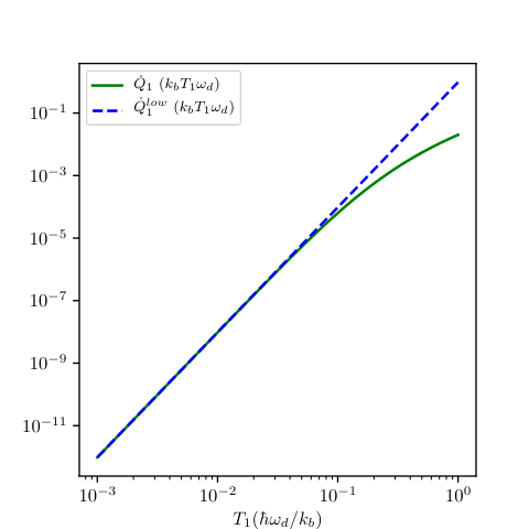
| (36) |
Due to the scaling with temperature, this expression is reminiscent of the Stefan-Boltzmann law for black-body radiation, which is a thermal equilibrium result. Indeed, a similar result would be obtained by considering two black bodies at thermal equilibrium but different temperatures which radiate towards each other. Thus, we see that non-equilibrium effects appear only at next-to-leading order in the low-temperature regime and are fully captured by Eq. (33). Also, we would like to point out that Eq. (36) is independent of the cutoff frequency. This is natural since for low temperatures only low frequency modes contribute to the heat current, while the cutoff frequency controls the high-frequency region of the spectral densities. In Fig. 3 we sketch the behavior of the total heat current when the bath temperatures are decreased. For low temperatures, we can see that the heat current is indeed well approximated by Eq. (36).
Turning to the regime of intermediate temperatures, where , we employ the following expansion of the digamma function for small values of ,
| (37) |
where is the Euler–Mascheroni constant. We then find the following high-temperature expansion of the quantum contribution
| (38) |
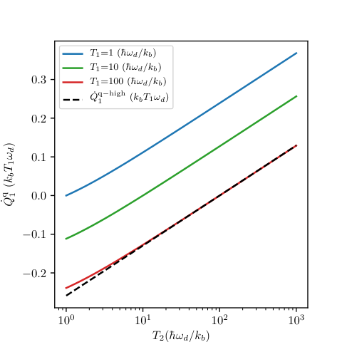
Surprisingly, we see that the dominant term does not necessarily vanish for . The reason for this is that under the constraints given in Eq. (29), one can assume that the temperature is high compared to the slow frequency scale , but it must remain low compared to the fast frequency scale . In other words, the temperature sits in the middle of the time scale separation associated to the overdamped regime. Thus, to the first non-trivial order the total heat current for high temperatures is,
| (39) |
Figure 4 shows the behavior of the quantum contribution with respect to the growth of the temperature. When both bath temperatures are increased, we can still observe a non-zero quantum correction to the heat currents.
V Conclusions
We have investigated the heat current between two overdamped quantum harmonic oscillators interacting with local thermal baths, without invoking the weak coupling and Markovian approximations. Exploiting the time-scale separation associated to the overdamped regime we were able to obtain closed analytical expressions for the heat current, identifying quantum and classical contributions. These analytical results might offer a useful benchmark to test Markovian embedding schemes or other approximate methods, for example the one developed in Mascherpa et al. 2020. Although our results are valid for general harmonic systems, we have explicitly considered an electronic implementation. This is justified by the fact that low-temperature electronic circuits are a promising platform to study quantum energy transport Pascal et al. 2011; Pekola 2015; Ronzani et al. 2018; Li et al. 2019. We found that in the overdamped regime a range of intermediate temperatures opens up between the low-temperature and high-temperature regimes usually considered. Our results indicate that in this intermediate range there are significant quantum corrections to the classical heat current, which survive even if the temperatures are high compared to the only relevant frequency scale of the system dynamics.
References
- Hannes and Till (1996) R. Hannes and F. Till, Springer-Verlag (1996), 10.1007/978-3-642-61544-3.
- Esposito and Haake (2005) M. Esposito and F. Haake, Phy. Rev. A 72, 063808 (2005).
- Pechukas et al. (2000) P. Pechukas, J. Ankerhold, and H. Grabert, Annalen der Physik 9, 794 (2000).
- Ankerhold et al. (2001) J. Ankerhold, P. Pechukas, and H. Grabert, Phys. Rev. Lett. 87, 086802 (2001).
- Dillenschneider and Lutz (2009) R. Dillenschneider and E. Lutz, Phys. Rev. E 80, 042101 (2009).
- Esposito et al. (2015) M. Esposito, M. A. Ochoa, and M. Galperin, Phys. Rev. Lett. 114, 080602 (2015).
- Esposito et al. (2010) M. Esposito, K. Lindenberg, and C. V. d. Broeck, New Journal of Physics 12, 013013 (2010).
- Esposito and Ochoa (2015) M. Esposito and M. Ochoa, Maicol A. andGalperin, Phys. Rev. B 92, 235440 (2015).
- (9) N. Bergmann and M. Galperin, arXiv:2004.05175 [cond-mat] arXiv:2004.05175.
- Bruch et al. (2016) A. Bruch, M. Thomas, S. Viola Kusminskiy, F. von Oppen, and A. Nitzan, Phys. Rev. B 93, 115318 (2016).
- Katz and Kosloff (2016) G. Katz and R. Kosloff, Entropy 18, 186 (2016).
- Seifert (2016) U. Seifert, Phys. Rev. Lett. 116, 020601 (2016).
- Freitas and Paz (2017) N. Freitas and J. P. Paz, Phys. Rev. E 95, 012146 (2017).
- Perarnau-Llobet et al. (2018) M. Perarnau-Llobet, H. Wilming, A. Riera, R. Gallego, and J. Eisert, Phys. Rev. Lett. 120, 120602 (2018).
- Bruch et al. (2018) A. Bruch, C. Lewenkopf, and F. von Oppen, Phys. Rev. Lett. 120, 107701 (2018).
- Dou et al. (2018) W. Dou, M. A. Ochoa, A. Nitzan, and J. E. Subotnik, Phys. Rev. B 98, 134306 (2018).
- Haughian et al. (2018) P. Haughian, M. Esposito, and T. L. Schmidt, Phys. Rev. B 97, 085435 (2018).
- Strasberg (2019) P. Strasberg, Phy. Rev. E 100, 022127 (2019).
- Martinez and Paz (2013) E. A. Martinez and J. P. Paz, Phys. Rev. Lett. 110, 130406 (2013).
- Freitas and Paz (2014) N. Freitas and J. P. Paz, Phys. Rev. E 90, 042128 (2014).
- Vool and Devoret (2016) U. Vool and M. H. Devoret, International Journal of Circuit Theory and Applications 45, 895 (2016).
- Girvin (2014) S. M. Girvin, Oxford University Press (2014), 10.1002/cta.2359.
- Gaul and Büttner (2007) C. Gaul and H. Büttner, Phys. Rev. E 76, 011111 (2007).
- Asadian et al. (2013) A. Asadian, D. Manzano, M. Tiersch, and H. Briegel, Phy. Rev. E 87, 012109 (2013).
- Nicacio et al. (2015) F. Nicacio, A. Ferraro, A. Imparato, M. Paternostro, and F. Semião, Phys. Rev. E 91, 042116 (2015).
- Freitas et al. (2015) N. Freitas, E. A. Martinez, and J. P. Paz, Physica Scripta 91, 013007 (2015).
- Riseborough et al. (1985) P. S. Riseborough, P. Hanggi, and U. Weiss, Phys. Rev. A 31, 471 (1985).
- Mascherpa et al. (2020) F. Mascherpa, A. Smirne, A. D. Somoza, P. Fernández-Acebal, S. Donadi, D. Tamascelli, S. F. Huelga, and M. B. Plenio, Phys. Rev. A 101, 052108 (2020).
- Pascal et al. (2011) L. M. A. Pascal, H. Courtois, and F. W. J. Hekking, Phys. Rev. B 83, 125113 (2011).
- Pekola (2015) J. P. Pekola, Nat. Phys. 11, 118 (2015).
- Ronzani et al. (2018) A. Ronzani, B. Karimi, J. Senior, Y.-C. Chang, J. T. Peltonen, C. Chen, and J. P. Pekola, Nat. Phys. 14, 991 (2018).
- Li et al. (2019) H. Li, L. J. Fernández-Alcázar, F. Ellis, B. Shapiro, and T. Kottos, Phys. Rev. Lett. 123, 165901 (2019).
Appendix A Coupled RLC circuits Hamiltonian
The Hamiltonian of a LC circuit can be written such that
| (40) |
In this notation, and will play the role of momentum and position conjugate variables, respectively. To quantize the LC circuit, we need to replace the classical variables of the Hamiltonian (40) with their quantum counterparts. In the other words, the Poisson bracket of the flux and charge in the circuit would be
| (41) |
As shown by Dirac the value of a classical Poisson bracket imposes it’s corresponding quantum commutator
| (42) |
Thus, we see that transforming the classical Hamiltonian into its quantum version will also be backed by the uncertainty relation between flux and charge variables as they play the role of position and momentum, respectively.
The dissipative part would be the resistor attached to the LC circuit. However, adding the Hamiltonian of this part is not trivial. To write the full Hamiltonian of a RLC circuit, we will employ the Caldeira-Leggett model for the Brownian motion. The resistor can be considered as a circuit consisting of an infinite array of independent LC circuits each playing the role of harmonic oscillators of the bath (Fig. 5).

Considering the RLC circuit of Fig. 5, we can write the full Hamiltonian describing the circuit such that
| (43) |
In the above expression, the flux variable and correspond to the node fluxes. The node flux is defined as the time integral of the voltage along the path connecting the node and the ground. and are also the charge in the capacitor and . The last term in the Hamiltonian can also be realized as the normalizing term to ensure that there will be no inconsistency in the minimum of the potential energy.
Next, we will magnetically couple two quantum RLC circuits by putting them into the proximity of each other. Indeed, the coupling occurs due to the presence of a flux running in one circuit which is caused by the other inductor. This leads to the mutual inductance between the two inductors of the two circuits. Before considering two coupled RLC circuits, we first look at two simple coupled circuits of Fig. 6. We denote the total flux passing through -th circuit by with . The total flux is the sum over the flux produced by the inductor and the mutual flux between the circuits with . We may write this such that
| (44) |
To find the Hamiltonian of the coupled circuits, we use the Kirchhoff’s law for voltages to obtain
| (45) | ||||
| (46) |
Where and are the voltages associated with the two capacitors and and are the currents for each circuits. For mutual flux we can write
| (47) |
where is the mutual inductance between the two circuits and it can be proved that .

To calculate the energy stored in the two coupled circuits, we first assume that and is increased up to an arbitrary value . Then the power stored in the left circuit is
| (48) |
Then the total energy will be
| (49) |
Now, we assume that is constant and we change from zero to . Since is changing, the mutual voltage induced in the left circuit is and therefore the total power will become
| (50) |
thus the energy stored in the circuit can be written as
| (51) |
We can write the total energy of the circuits as the sum over and such that
| (52) |
Adding the energy with respect to the capacitors to this energy we can write the Hamiltonian as
| (53) |
Above, we replaced arbitrary currents and by and . We can see that is the coupling constant between the two circuits.
To find the Hamiltonian of the two RLC circuits, similar to what we did in Eq. (43) we attach two resistors to the both ends of the coupled LC circuits. We can replace currents in Eq. (53) with their flux variables by using the relation . Doing so the Hamiltonian of this model will then become
| (54) |
Next, we will eliminate the flux terms to write it in terms of the total flux . To do so we use the bellow relations between the fluxes
| (55) | ||||
| (56) |
These relations together with Eq. (44) gives
| (57) |
We can now replace these transformation in Eq. (A) to find the Hamiltonian of our model such that
| (58) |
Appendix B Steady state heat currents
Using the Heisenberg equations of motion, we can find the integro-differential equation for each variables of the system and then they can be solved using the Green’s function matrix of the system which satisfies the integro-differential equation,
| (59) |
with the initial condition .
Assuming that the Green’s function is an exponentially decaying function with respect to , the correlations functions between the system variables, i.e and , will be independent of the initial state of the total system for large . To capture the correlation functions, we use covariance matrix such that
| (60) |
In terms of the Green’s function , one can obtain
| (61) |
where
| (62) |
denotes the noise kernel. Also , and and is the th derivative of . Considering a situation in which, the spectral density is a continuous function of we can write the covariance matrix for the steady state limit, i.e such that
| (63) |
Where is the covariance matrix in the asymptotic state, is the Fourier transform of the noise kernel and is the Laplace transform of the Green function which can be obtained using Eq. (59) such that
| (64) |
where is the Laplace transform of .
Now we turn to analyse the heat flow thorough the system. Since there exists no deriving in the system, the heat current is directly related to the change in the mean value of the energy of the system and for the steady state one can write
| (65) |
To calculate the local heat current, we first write by using
| (66) |
where . Replacing this into Eq. (61) we can see in the limit we can write
| (67) |
thus we will have
| (68) |
Replacing this equation into Eq. (65) we will have the local heat current expression for steady state limit as
| (69) |
Where we have used the fact that . The heat transfer matrix element is written such that
| (70) |
Here we have . Replacing this relation into the above equation, we can see that because is a symmetric matrix and is anti-symmetric and the trace of their product will be vanishing. That said we can write the heat transfer matrix as
| (71) |
To expand the above relation a bit further, we first take the Laplace transform of Eq. (59) such that
| (72) |
Writing in terms of we have
| (73) |
Replacing the above equation into Eq. (71) with , we will have
| (74) |
The first term vanishes because for . The second will also be vanishing because it is a product of two symmetric and anti-symmetric matrices. In the third term, the matrix is hermitian so that we only have to calculate . Thus we have
| (75) |
Inserting this matrix back into Eq. (69) we will have
| (76) |
Appendix C Quantum correction to the heat current
To calculate the quantum contribution to the heat currents we will analytically solve the integral in Eq. (26). To do so, we will have to take into account the poles of the digamma function in addition to the poles of . In fact the poles of the function are all located on the lower-half of the imaginary axis, i.e . The poles of the heat transfer matrix element, and their conjugates are on the imaginary axis. However, since we would like to exclude the contribution from the digamma function poles, we choose the integration contour to run on the upper-half plane which only covers . Thus, we can write the integral such that
| (77) |
The first integral is done over the contour c in Fig. 7 by using the residue theorem. The second integral is the contribution for . In this limit we need to expand the digamma function using
| (78) |
for . Since the integrand is vanishing as then we only need to keep the logarithmic term in the asymptotic digamma functions. Replacing this expansion into the second integral in Eq. (77) we will have
| (79) |
We change the variable and we integrate over the semi-circle on the upper-half plane for and , thus we will have
| (80) |
Hence, by adding the above result and the integral over the contour we will obtain Eq. (26).