Cosmicflows-4: The Catalog of 10000 Tully-Fisher DistancesJournal: ApJ
Abstract
We present the distances of 9792 spiral galaxies lying within 15,000 using the relation between luminosity and rotation rate of spiral galaxies. The sample is dominantly, but not exclusively, drawn from galaxies detected in the course of the ALFALFA H i survey with the Arecibo Telescope. Relations between H i line widths and luminosity are calibrated at SDSS u, g, r, i, z bands and WISE W1 and W2 bands. By exploiting secondary parameters, particularly color indices, we address discrepancies between measured distances at different wave bands with unprecedented detail. We provide a catalog that includes reduced kinematic, photometric, and inclination parameters. We also describe a machine learning algorithm, based on the random forest technique that predicts the dust attenuation in spirals lacking infrared photometry. We determine a Hubble Constant value of (stat.), with potential systematics up to 3 km s-1 Mpc-1.
Keywords:
Galaxy distances (590); Spiral galaxies (1560); Galaxy photometry (611); Hubble constant (758); H I line emission (690); Large-scale structure of the universe (902); Inclination (780); Sky surveys (1464); Catalogs (205); Distance measure (395); Random Forests (1935);I Introduction
The Cosmicflows program is an ongoing project to map the structure of the universe from departures in the motions of galaxies from the mean cosmic expansion. Galaxies are test particles experiencing ”peculiar velocities” in the line of sight due to the distribution of (mostly dark) matter: , where is the radial velocity, is the radial distance of a galaxy and is the Hubble constant.
Errors on individual measurements are substantial, but meaningful signals can be discerned because of coherence in the motions of adjacent systems. A robust modeling of the complexities of large-scale structure requires dense coverage of space with many thousands of accurate distance measurements.
Over the course of successive releases, Cosmicflows has expanded in distance and density coverage. With Cosmicflows-3, the most important incrementation involved the inclusion of the Fundamental Plane measures from the Six Degree Field Redshift Survey (Magoulas et al. 2012; Springob et al. 2014). This component is restricted to ; hence, whereas Cosmicflows-2 was relatively deficient in the south celestial hemisphere, Cosmicflows-3 is heavily weighted toward coverage of the south (Tully et al. 2013; Tully et al. 2016).
The next release, Cosmicflows-4, will largely redress the hemispheric imbalance. This paper presents the most important new contribution to the forthcoming Cosmicflows update. The methodology for obtaining galaxy distances involves the correlation between galaxy luminosities and rotation rates, known as the Tully-Fisher Relation (Tully & Fisher 1977, TFR; ). Thanks to the completion of the Arecibo Legacy Fast ALFA Survey (ALFALFA; Haynes et al. 2011; Haynes et al. 2018) the sky has now been covered in the declination range with sufficient sensitivity to have detected many thousands of galaxies extending to . Concurrently, photometry over most of this same sky has been made available by the Sloan Digital Sky Survey (Alam et al. 2015, SDSS; ) providing imaging in the five optical bands ,g,r,i and z. Complementary infrared photometry is available from the all-sky observations of the Wide-field Infrared Satellite Explorer (Wright et al. 2010, WISE; ), imaging in the W1 and W2 (3.4 and 4.6 m) bands.
The availability of seven-band photometry spanning a decade in wavelengths (m) permits a considerably refined calibration of the TFR. In Kourkchi et al. 2019 (hereafter K19) there was exploration of two important ingredients: the definition of inclinations and the properties of internal reddening as a function of inclination. Then, in Kourkchi et al. 2020 (hereafter K20) the TFR was calibrated in the seven photometric bands with slopes determined from galaxies in 20 clusters and the zero-point set by 64 galaxies with Cepheid and/or tip of the red giant branch distances. In the studies of both these papers, the calibrations benefited from information provided by such distance-independent parameters as colors, surface brightness, and relative H i to optical-infrared fluxes.
In this paper, we use the luminosityline-width correlations to calculate the distances of almost 10,000 spirals. This effort involves a mix of SDSS optical and WISE infrared photometry. We investigate discrepancies and color-dependent systematics and uncertainties that are inherent in the utilization of TFRs across multiple bands.
II Data
There are roughly power-law relations between the absolute luminosities of spiral galaxies at optical and near infrared wavelengths and their rotation rates probed through the width of the 21cm emission line of their neutral hydrogen (H i ) content. Therefore, the existence of high signal-to-noise H i data is one of the essentials in the compilation of our catalog. Next, we need to know the inclinations of target spirals. Systems with spatial orientations approaching face-on are not useful, because of the ambiguity in deprojecting to full rotation rates. Finally, we need high-quality imaging data to measure apparent magnitudes and other photometric metrics.
The following conditions are adopted to initially select a set of 19,905 potential candidates, all of which have radial velocities within 15,000 : (1) morphological types Sa or later; (2) inclinations estimated to be greater than from face-on, based on axial ratios cataloged in HyperLEDA11 1 http://leda.univ-lyon1.fr/ (Paturel et al. 2003); (3) high-quality H i measurements as explained in §II.1; (4) no suggestion of tidal distortion, H i confusion, or gross anomaly. These limitations, plus an assessment of the quality condition of the optical/infrared photometry, reduces the number of candidates to 13,434. Further pruning based on the results of our more accurate inclination measurements, described in §II.3, leaves us with 10,737 galaxies.
II.1 H i Data
We accept the H i line widths and fluxes from four resources: (1) Our primary source (78% of cases) is the All Digital H i catalog (ADHI), which has been collected over the course of the program (Courtois et al. 2009; Courtois et al. 2011b, A. Dupuy et al., in preparation) and is accessible online at the Extragalactic Distance Database (EDD) website22 2 http://edd.ifa.hawaii.edu; catalog “All Digital H i ”. (2) Most of the remainder (19% of cases) are given by the Arecibo Legacy Fast ALFA Survey (ALFALFA; Haynes et al. 2011; Haynes et al. 2018) with coverage over the declination range degrees. Neutral hydrogen spectral information provided by the ALFALFA 40% early data release is already included in ADHI but information only made available with the 100% ALFALFA data release has not yet been ingested into ADHI. (3) In a small number of cases (50 galaxies, i.e. 0.5% of the total cases), line widths are uniquely provided by the Springob/Cornell H i catalog (Springob et al. 2005). (4) For 3%, the source is the Pre Digital H i catalog that is available in EDD, which provides information from early analog H i line profiles, either from single beam or interferometric observations (Fisher & Tully 1981; Huchtmeier & Richter 1989). Generally, this old material must be used in the cases of nearby galaxies that are much larger than the beam sizes of currently operational radio telescopes.
ADHI provides a measure of the H i line widths, , that robustly encodes the rotation rates of spirals along the line of sight. The value of is derived from the observable quantity , the width of the H i line profile at 50% of the average H i flux within the range that covers 90% the total H i flux, and is adjusted for spectral resolution and redshift. Contributions to ADHI derive from observations with diverse facilities (those at Green Bank Observatory, Arecibo, Parkes, Nancay, and Effelsberg) but no matter which sources they are from, they are carried through our pipeline that takes account of differences in spectral resolution and smooths consistently (Courtois et al. 2009; Courtois et al. 2011b). As mentioned, ADHI includes material from the ALFALFA 40% release, analyzed by us in our standard way. The consequence is a large overlap in measurements of ALFALFA profiles between ADHI and those of the ALFALFA team that permits a reliable transformation of the ALFALFA 100% line widths into the ADHI system.
To be compatible with the ADHI values, we transform ALFALFA line widths, , using , which is derived for galaxies covered by both catalogs. Springob/Cornell provides values for , that are adjusted using and are then converted into values based on the ADHI standard procedure explained by Courtois et al. 2009. The Pre Digital H i catalog provides , the width at 20% of the H i profile maximum. We translate values to based on the relation described by Courtois et al. 2009.
In the regime of dwarf galaxies, the TFR scatter increases substantially. Such faint galaxies are only accessible nearby and are considered less useful for our purposes. Hence, we impose a low-luminosity cutoff at . Accordingly, we can safely reject galaxies with less than because such cases will inevitably lie faintward of the luminosity cut.
H i detections of poor quality are rejected. ADHI values are considered if their associated uncertainties are less than or equal to . We discard candidates with anomalous, confused, or low signal-to-noise line profiles. In the cases of ALFALFA line widths, we set the threshold of , which is reasonably compatible with our condition for accepting ADHI data.
To extract H i information, we assign the highest priority to ADHI and ALFALFA catalogs and the lowest priority to Pre Digital H i catalog. For galaxies that are listed in both ADHI and ALFALFA catalogs, we take the average of H i flux and line width values. Out of 10,737 candidates that meet all of our requirements, 8333 spirals have H i data in the ADHI catalog, 5120 galaxies are introduced by ALFALFA, and 3255 galaxies have H i measurements in both catalogs. The H i data for 236 galaxies is provided by Springob/Cornell catalog, and for 302 galaxies we use information from the Pre Digital H i catalog. We convert the H i flux within the 21 cm line profiles, , given in the units Jy, to an H i magnitude, , using .
II.2 Imaging Data
For the optical photometry of our galaxies, we use the SDSS DR12 data release (York et al. 2000). For each galaxy with available SDSS data, we download all the single exposure cutouts at u,g,r,i and z bands33 3 Our data acquisition pipeline is accessible online at https://github.com/ekourkchi/SDSS_get, which are drizzled and combined using MONTAGE, an astronomical application to assemble images (Jacob et al. 2010). Our pipeline provides galaxy cutouts at all ugriz passbands with a spatial resolution of 0.4” pixel-1. For the infrared part, we obtain the W1 (3.4) and W2 (4.6) images of the WISE survey (Wright et al. 2010), from the NASA/IPAC infrared science archive (IRSA). We generate the cutouts of galaxy images by drizzling single exposure frames using version 3.8.4 of the Image Co-addition with Optional Resolution Enhancement (ICORE) software (Masci & Fowler 2009; Masci 2013). Our final co-added infrared images have a spatial scale of 1” pixel-1. All of our optical and infrared images are calibrated to produce magnitudes in the AB system. For more detailed information on how we conduct our image preprocessing, please refer to §2.2 and 2.3 of K19.


II.2.1 Photometry
For the surface photometry of our galaxies, we use the photometry pipeline that was originally developed to assemble the WISE Nearby Galaxy Atlas (WNGA; M. Seibert et al. 2020, in preparation). We added flexibility to the WNGA pipeline and improved the efficiency of its user interface, providing easily accessible tools that facilitate the manual procedures required in our photometry program. In the photometry process, the galaxy light profile is derived within concentric elliptical apertures, with geometrical information such as the center, size, and axial ratio initially taken from the HyperLEDA44 4 http://leda.univ-lyon1.fr/ (Paturel et al. 2003) catalog. The aperture is later repeatedly adjusted either by visual inspections, or with the aid of SExtractor (Bertin & Arnouts 1996) and/or the galaxy isophots visualized by DS9 (Joye & Mandel 2003).
The sky background is evaluated within a large annulus far from the photometry aperture. All foreground stars are initially masked automatically—however, further manual masking is required for companion extended objects, point sources that are not automatically recognized, and other features such as diffraction spikes. On the other hand, the software tends to mask the blue star forming clumps in spiral arms, which needed to be unmasked. The resulting light curve is calculated radially in increments of 3” for u,g,r,i,z bands and 6” for W1 and W2 bands.
The quality of the generated light profiles and growth curves are visually inspected. If necessary, further masking/unmasking and adjustments of the aperture and the background estimation annulus are applied iteratively until the growth curve converges. At the end of each iteration, the resulting luminosity growth curve and surface brightness profile is evaluated for abnormal changes in luminosity due to unmasked objects or poor subtraction of the sky level.


In some cases, the galaxy image is superimposed with many other sources in crowded regions, such as near the Galactic plane, which makes masking and sky-subtracting very challenging. Furthermore, pollution by unresolved background objects may affect our evaluated sky level. We attempt to address these complexities by means of visual inspections and playing with the masking thresholds. Tackling this issue is simpler for our SDSS cutouts, owing to their high spatial resolution (0.4” pixel-1) and the minimal sky level that remains from the initial SDSS sky subtraction. The large-resolution elements of the WISE images (6”) make it more difficult to accurately evaluate the sky background. At infrared bands, our standard routine produces reasonable results. However, for galaxies with a nonconvergent curve of growth, we need to interactively alter the background level by a few percent of the initial estimations in order to eliminate surface brightness anomalies and force the curve of growth to converge.
As examples, Figures 1 and 2 display photometry apertures, masks, and light curves for NGC 881 (PGC 8822). Our photometry results, including light curves and all measured quantities, are publicly available online through the EDD55 5 To query the results of our SDSS photometry, go to http://edd.ifa.hawaii.edu/cf4_photometry/get_sdss_cf4.php, and enter the galaxy name or its PGC number. In a similar fashion, you can access to our WISE photometry results at http://edd.ifa.hawaii.edu/cf4_photometry/get_wise_cf4.php. .
Our photometry pipeline calculates two versions of “total magnitude”. (1) The asymptotic magnitude is derived within the aperture radius, beyond which the curve of growth is flat (the horizontal dotted lines in the top right panel of Figures 1 and 2). Asymptotic radii are robust parameters that are independent of the user’s choice of aperture. (2) An isophotal magnitude calculated within 25.5 mag arcsec-2 with augmentation calculated from extrapolating the extension of an exponential fit of the galaxy disk to infinity (Tully et al. 1996; Neill et al. 2014). We found that the average discrepancy between these two types of magnitude is no worse than mag in all bands for the brightest objects, and it always remains below mag for fainter galaxies at all passbands—except for the u band, which has lower quality ( mag). Our final results are insensitive to the magnitude choice, and we choose to use asymptotic magnitudes that are derived with no assumptions about galaxy type.

II.2.2 Adjusting apparent magnitudes
At any passband , the raw total apparent magnitude of each galaxy, , is corrected to account for dust obscuration in the Milky Way, , and dust attenuation in the target galaxy along the line of sight, , and the effect of spectral redshift on the galaxy luminosity at each band (-correction), . The adjusted magnitude is given as
| (1) |
Here, is an adjustment that accounts for the diffuse scattered light from extended objects (galaxies) lost from the fixed-size apertures used in establishing the photometric calibration with point sources (stars). There is a detailed discussion of the derivation of , , and in §2.5 of K19.
In K19, it is shown that the amplitude of dust obscuration in the host galaxy, , can be modeled as a function of (1) the galaxy physical properties that are probed by the galaxy observables and (2) the galaxy spatial inclination. The description of is given as
| (2) |
where is a monotonically increasing function of the inclination angle from face-on, i66 6 Symbol i should not to be confused with the photometric passband. (see §II.3 for the full discussion on the measurement of inclinations), described by
| (3) |
where is a wavelength-dependent parameter of the obscuration model. The dust attenuation factor, is calculated using a third-degree polynomial function of , the main principal component of the galaxy observables, constructed based on the H i line width adjusted for inclination using , a pseudo-color calculated based on the H i 21 cm and W2 magnitudes, , and the average surface brightness of galaxy at W2 band within the effective radius that is corrected for the geometric effect of inclination, . The relation to calculate is expressed as
| (4) |
and is given by
| (5) |
where and are the semimajor and semiminor axes of the photometry aperture. It should be kept in mind that the galaxy effective surface brightness is derived from its total magnitude and the effective radius, , following
| (6) |
There is a full discussion in K19 regarding the calculation of .
A problem arises if there is missing information. SDSS photometry is only available across part of the sky. WISE photometry is available, in principal, across the entire sky, but the time-consuming effort to acquire WISE photometry for all potential targets has not been completed. In the Appendix B there is discussion of a predictive algorithm that provides acceptable substitutions for calculations of attenuation.
Figure 3 illustrates the distribution of our galaxies color coded based on their photometry coverage. The ALFALFA survey running excluding the zone of avoidance, strongly overlaps with the SDSS footprint.

II.3 Inclination
Inclinations are a significant source of error in the TFR. Inclinations enter into the determinations of both magnitudes and line widths. The lesser problem is with magnitudes; the issues in that regard are discussed in §II.2.2 and Appendix B. Corrections to line widths introduce greater uncertainties and potential systematics.
If the image of a spiral galaxy is the projection of a perfect disk with an oblate spheroidal shape, then the inclination, i, can be derived from the axial ratio, , following the formulation , where is the thickness of the spiral disk as observed edge-on. The choice of has been used in previous studies (Tully et al. 2013). We adopted the analogous relation in §4 of K19 to formulate the internal dust attenuation of spiral galaxies, where we let be a free parameter that depends on the passband. In that formulation, is not constant, but instead is treated just as a hyperparameter without direct geometrical implications.
Ellipticity-derived inclinations can be misleading for various reasons. The disks of spirals might be warped, or axially asymmetric due to tidal interactions. The bulges of large spirals dominate their disks, inflating the observed ratio , especially at redward passbands. Extreme contrast in the surface brightness of disk components, such as bars, arms, and irregularities, can alter the shape of the photometry aperture and lead to large errors. Otherwise, confusion can simply originate from the nontrivial orientation of strong spiral components relative to the major axis of projection on the sky (spiral arms opening onto the minor vs the major axis). Previously, the statistical determinations of the inclinations of large samples of spirals have been unsatisfactory.
In this study, we pursue a different approach that relies on the judgment of the human eye to evaluate galaxy inclinations. Fortunately, a large fraction of spirals have well-defined inclinations defined by their axial ratios. These good cases provide a baseline with sufficient coverage of morphological types and inclinations over the range of ∘that concerns us.
The details of our procedures are described in §2.5 of K19, where there is a discussion of the online graphical tool, Galaxy Inclination Zoo (GIZ)77 7 http://edd.ifa.hawaii.edu/inclination/index.php. Users of the interface are asked to situate a target galaxy within a lattice of galaxies with established inclinations. The interface was initially validated by two of us (E.K. gave attention to the entire sample and R.B.T. looked at about half). The site was then opened up to colleagues and students, with initially intensive and progressively more relaxed training.


II.3.1 Evaluating User’s Measurements
Initially, the performance of the tool was evaluated, for a significant fraction of galaxies, by two of the authors. First, E.K. and R.B.T. gave careful attention to more than 2000 spirals involved in the sample used for the study of the dust attenuation of K19 and the TF calibrators study of K20. The results are in agreement, with root-mean-squared (rms) differences between E.K. and R.B.T. of ∘with no meaningful systematics. Subsequently, E.K. used the tool to measure the inclinations of our 20,000 tentative candidates.
In order to improve the accuracy of our final estimations, we opened the tool to 10 different users, including graduate and undergraduate students. We provided them with multiple sets of galaxies with sufficient overlaps that allowed us to assess the consistency of the measurements and correct for user-dependent systematics. Later, we opened the online tool to a larger number of citizen scientist and amateur astronomers across the world, whose participation helped us to improve our number statistics and efficiency.
The downside of adding the multiple measurements of different users is the possibility of introducing biases due to human mistakes. To remove the user-driven systematics, we build up our compendium of good measurements by adding the measured inclinations of each user individually. In the beginning, we adopt the measurements of E.K. and R.B.T. as acceptable inclinations, and for each galaxy, we use the median of the measured values as a benchmark to assess new measurements. For the results of a user to be accepted, we first compare with the median of the previous good measurements in our ensemble for galaxies in common. In a case of large discrepancies, we reject all the user measurements. Small discrepancies are modeled by fitting linear relations, allowing us to correct the new measurements prior to integrating them into our ensemble. As an example, Fig. 4 plots the results of a user for 310 galaxies versus the median value of all inclinations measured by different users except for the chosen user. In the left panel of this figure, it is seen that the raw measurements are clearly overestimated at the face-on end. The dashed line shows our linear fit to this inclination-dependent bias, used to produce the corrected inclinations shown in the right panel. While users continue their work, the number of cross-evaluations increases, and so the number of reliable measurements does as well. We iteratively modify the linear-correcting relations, until reaching convergence. We also acknowledge the differences in the users’ performances by considering weighted numbers toward the calculation of the median inclinations. We use integer weight numbers that are no greater than 4. We derive weight number in an iterative process based on user experience, the level of needed corrections (according to the slope of the fitted line), and/or the rms scatter of differences between raw measurements and the median values.
The left panel of Fig. 5 plots the distribution of the median evaluated inclinations for all the 10,737 accepted spirals in our program. There is an excess in the most edge-on bin because, in the portion of the H i sample derived from individual pointings (the non-ALFALFA portion), edge-on systems have been favored. The distribution of the number of measured inclinations for these spirals is illustrated in the right panel of Fig. 5. We ended up with less than three measurements in 925 cases, as users (other than E.K. and R.B.T.) rejected galaxies for invalid reasons.
Increasing the number of individual measurements for each galaxy improves the results of the evaluated inclinations. Nevertheless, the manual evaluation is a tedious task and requires long hours of visual inspections by multiple users. In our program, we required each galaxy to be evaluated by three different users. To quantify the consistency of the final results, we randomly divide all participants in two groups, A and B, in such a way that the total number of measurements done by each group is almost the same. Fig. 6 compares the median evaluated inclinations of the galaxies inspected by both groups. Each galaxy has at least three separate measurements by the users of each group. The scatter of discrepancies across the entire range of inclinations is better than ∘and no inclination dependent systematic is apparent.


II.3.2 Uncertainties
Fig. 6 reveals that the scatter of deviations from the equality line is smaller for the edge-on galaxies and it increases toward the face-on spirals. To quantify the average uncertainty of the users measurements as a function of inclination, Fig. 7 plots the deviation of all user-evaluated inclinations for all individual galaxies from the median estimated inclinations. In this figure, each blue point represents one galaxy whose inclination is evaluated by one user, with being the median of all measurements for that galaxy. In this analysis, we assume that the values are the correct estimations of inclination, and hence we use them as a reference to evaluate the level of uncertainty introduced by users. In Fig. 7, red filled points display the median and 1 standard deviation of blue points within ∘bins of . In agreement with our observation in Fig. 6, the scatter of the users’ measurements is small at large inclinations and gradually increases as the inclination angle decreases. For spirals more edge-on than 88∘, the user-evaluated inclinations are consistent within 1∘error bars, whereas for galaxies with inclinations more face-on than 50∘, the scatter of the measured inclinations is ∘.
Providing a more detailed examinations, Fig. 8 plots the distribution of measurement discrepancies, , within inclination intervals of 5∘. In each panel of Fig. 8, the black vertical dotted lines give the boundaries that exclude 34% of the measurements at each extremity from the median, which is zero by definition.
Except for the top left panel of this figure, , the other distributions look almost symmetrical. Therefore, we calculate by averaging the 1 right and left wings of histograms.
The inferred inclination-dependence of user measurements from Figures 7 and 8 are consistent. For spirals that are more edge-on than 88∘, the error is about 1∘. It is no worse than 2∘for inclinations larger than 85∘. The ambiguity is about 3∘for measurements in the range 70∘85∘, and it is no worse than 4∘for spirals that are more edge-on than 50∘. Our error evaluation for inclinations between 45∘and 50∘is not robust, owing to the small number of galaxies in our sample and the consequently small number of measurements in this range. We adopt a conservative uncertainty of 5∘for spirals more face-on than 50∘. We adopt these uncertainty values as a minimum floor for errors of reported inclinations. For an individual galaxy, the quoted error is the larger of these minimum values and the standard deviation of all averaged measured inclinations for that galaxy.

In Fig. 9, using a subset of common galaxies, we compare our derived inclinations with those tabulated in Neill et al. 2014 that are derived based on axial ratios. Both measurements seems to be in good agreement on average, within an rms uncertainty of about ∘. However, as discussed earlier, axial ratios are not good inclination estimators, as they might be subject to morphological peculiarities. Thus, there is no expectation that the two different methods yield exactly the same results.
Our collection of carefully measured inclinations provides a rich data set for training a machine-learning algorithm, such as the Convolutional Neural Network (CNN) (LeCun et al. 1998; Krizhevsky et al. 2012), to replace the human eye in the future projects. To successfully instruct such a network to produce satisfactory results, a training set of order representative galaxies is required. Our entire sample is of such a size, and hence suitable for exploring machine-learning capabilities. Moreover, -body cosmological simulations such as Illustris (Nelson et al. 2015) provide exquisite images of projected spiral galaxies with known 3D orientations that could be of potential interest as training sets for inclination studies.
II.4 Data Catalog
Table 1 gathers together directly observed and adjusted data and inferred parameters for 10,737 spiral galaxies used in this study. Columns provide the following information.
(1) The ID number of the galaxy in the Principal Galaxy Catalog (PGC; http://leda.univ-lyon1.fr/).
(2) Common name.
(3) The measured inclination of the galaxy in degrees with error (see §II.3).
(4) Heliocentric velocity from H i observations.
(5) The H i line width adjusted to approximate twice the maximum rotation velocity, , with error, in .
(6) The logarithm of the inclination-corrected H i line width, calculated from , where i is the inclination angle presented in column 3, with error.
(7) The H i 21 cm magnitude calculated from the H i flux, , using , with error.
(8-12) The SDSS u,g,r,i and z total raw magnitudes in the AB system.
(13-14) The WISE W1 and W2 total raw magnitudes in the AB system.
(15) The axial ratios of the elliptical photometry apertures used for the photometry of SDSS images, where and are the semi-major and semi-minor axes of the elliptical aperture, respectively.
(16) Analogous to 15 but for the photometry apertures of the WISE images.
(17-23) The semi-major axes of apertures that enclose half the total light of galaxies at optical/infrared bands in arcmin.
(24-30) Optical/infrared magnitudes corrected for Milky Way obscuration, redshift correction, and aperture effects, based on the corresponding raw magnitudes listed in columns (8-14).
(31-37) The dust attenuation corrections at optical/infrared bands, calculated from Equation2, with errors.
(38-44) The magnitudes after correcting for the effect of global dust obscuration, .
(45) The predicted value for the W2-band magnitude based on the optical photometry and other observable features of the galaxy (discussed in the Appendix B).
(46-52) Host dust attenuation factors as defined in Equation 2, with blank entries for galaxies with missing infrared photometry.
(53-59) The predicted dust extinction factors calculated using , the predicted W-band magnitude defined in Appendix B.4.
(60-66) The predicted dust extinction of hosts corresponding to columns (52-58).
(67) The main principal component based on the W2-band photometry calculated as given by Equation 4, with error.
(68) The main principal component derived based on the predicted value for W2-magnitude.
(69) The main principal component derived for the W1 band. This parameter is useful for galaxies with poor W2-band photometry. Here, is approximated by (K19).
(70-71) The manually assigned quality for the photometry of SDSS and WISE images. The quality grade ranges from for the poorest quality (or missing data) to for the best quality.
(72) An integer number between 0 and 2 that specifies what parameters are used for calculation of the dust obscuration in the host galaxies ( if the predicted is used, if the observed W1-band magnitude is used and if the 2-band magnitude is used through the standard attenuation formulation as discussed in §II.2.2).
| PGC | Name | g | r | i | z | W1 | W2 | |||||||||||||||
|---|---|---|---|---|---|---|---|---|---|---|---|---|---|---|---|---|---|---|---|---|---|---|
| (deg) | () | () | (mag) | (mag) | (mag) | (mag) | (mag) | (mag) | (mag) | (mag) | (′) | (′) | (′) | (′) | (′) | (′) | (′) | |||||
| (1) | (2) | (3) | (4) | (5) | (6) | (7) | (8) | (9) | (10) | (11) | (12) | (13) | (14) | (15) | (16) | (17) | (18) | (19) | (20) | (21) | (22) | (23) |
| 2 | UGC12889 | 524 | 5004 | 43716 | 2.7440.029 | 15.7130.185 | 11.86 | 12.49 | 0.66 | 0.51 | 0.51 | |||||||||||
| 4 | PGC000004 | 852 | 4458 | 1545 | 2.1890.014 | 16.6880.076 | 17.57 | 16.43 | 15.91 | 15.57 | 15.42 | 16.06 | 16.42 | 0.24 | 0.33 | 0.25 | 0.23 | 0.21 | 0.23 | 0.27 | 0.27 | 0.33 |
| 12 | PGC000012 | 823 | 6548 | 40019 | 2.6060.021 | 16.0710.185 | 13.60 | 14.20 | 0.36 | 0.25 | 0.25 | |||||||||||
| 16 | PGC000016 | 654 | 5667 | 29714 | 2.5150.025 | 17.2070.185 | 16.08 | 14.83 | 14.21 | 13.86 | 13.61 | 13.98 | 14.67 | 0.52 | 0.64 | 0.22 | 0.21 | 0.19 | 0.19 | 0.19 | 0.21 | 0.20 |
| 55 | UGC12898 | 803 | 4779 | 17910 | 2.2600.025 | 15.7570.076 | 16.82 | 16.08 | 15.71 | 15.50 | 15.40 | 16.18 | 16.60 | 0.32 | 0.46 | 0.28 | 0.23 | 0.23 | 0.22 | 0.22 | 0.22 | 0.26 |
| 68 | ESO538-017 | 574 | 7664 | 20618 | 2.3900.043 | 16.8830.185 | 16.31 | 15.24 | 14.86 | 14.69 | 14.49 | 14.99 | 15.49 | 0.66 | 0.66 | 0.16 | 0.17 | 0.16 | 0.15 | 0.15 | 0.19 | 0.19 |
| 70 | UGC12900 | 901 | 6800 | 4335 | 2.6360.005 | 15.0520.076 | 16.70 | 15.41 | 14.66 | 14.25 | 13.87 | 13.55 | 14.08 | 0.08 | 0.14 | 0.61 | 0.55 | 0.51 | 0.48 | 0.46 | 0.43 | 0.43 |
| 76 | UGC12901 | 684 | 6920 | 3905 | 2.6240.013 | 15.7780.076 | 15.83 | 14.39 | 13.65 | 13.26 | 13.00 | 13.21 | 13.77 | 0.45 | 0.47 | 0.34 | 0.29 | 0.27 | 0.26 | 0.25 | 0.30 | 0.32 |
| 92 | PGC000092 | 803 | 5376 | 1445 | 2.1650.016 | 15.9560.023 | 17.48 | 16.39 | 15.84 | 15.51 | 15.28 | 0.34 | 0.15 | 0.16 | 0.16 | 0.17 | 0.18 | |||||
| 94 | UGC12905 | 901 | 4098 | 18814 | 2.2740.032 | 16.0060.185 | 15.82 | 16.49 | 0.29 | 0.32 | 0.30 | |||||||||||
| 96 | UGC12903 | 813 | 14743 | 5599 | 2.7530.008 | 16.0750.076 | 16.68 | 15.18 | 14.45 | 13.99 | 13.73 | 0.26 | 0.32 | 0.30 | 0.26 | 0.25 | 0.23 | |||||
| 102 | IC5376 | 823 | 5048 | 4277 | 2.6350.007 | 15.4110.076 | 15.81 | 14.28 | 13.45 | 13.02 | 12.73 | 12.85 | 13.45 | 0.25 | 0.27 | 0.43 | 0.38 | 0.33 | 0.30 | 0.27 | 0.33 | 0.34 |
| 124 | UGC12913 | 862 | 6350 | 2526 | 2.4020.010 | 15.7820.076 | 17.23 | 15.85 | 15.26 | 14.96 | 14.76 | 15.18 | 15.75 | 0.23 | 0.29 | 0.29 | 0.32 | 0.31 | 0.30 | 0.30 | 0.32 | 0.34 |
| 128 | PGC000128 | 594 | 12559 | 2188 | 2.4060.024 | 16.8500.076 | 17.11 | 16.19 | 15.96 | 15.70 | 15.47 | 0.69 | 0.14 | 0.14 | 0.13 | 0.12 | 0.13 | |||||
| 146 | UGC12916 | 504 | 6360 | 1625 | 2.3250.029 | 16.7160.076 | 16.80 | 15.72 | 15.22 | 14.92 | 14.82 | 15.43 | 16.02 | 0.86 | 0.74 | 0.24 | 0.22 | 0.21 | 0.21 | 0.20 | 0.24 | 0.27 |
| PGC | ||||||||||||||||||||
|---|---|---|---|---|---|---|---|---|---|---|---|---|---|---|---|---|---|---|---|---|
| (mag) | (mag) | (mag) | (mag) | (mag) | (mag) | (mag) | (mag) | (mag) | (mag) | (mag) | (mag) | (mag) | (mag) | (mag) | (mag) | (mag) | (mag) | (mag) | ||
| (1) | (24) | (25) | (26) | (27) | (28) | (29) | (30) | (31) | (32) | (33) | (34) | (35) | (36) | (37) | (38) | (39) | (40) | (41) | (42) | |
| 2 | 11.90 | 12.53 | 0.010.00 | 0.010.00 | ||||||||||||||||
| 4 | 17.11 | 16.11 | 15.69 | 15.41 | 15.30 | 16.08 | 16.44 | 0.810.12 | 0.520.08 | 0.360.06 | 0.290.05 | 0.230.04 | 0.010.00 | 0.000.00 | 16.30 | 15.59 | 15.33 | 15.12 | 15.07 | |
| 12 | 13.64 | 14.24 | 0.050.01 | 0.010.01 | ||||||||||||||||
| 16 | 15.86 | 14.69 | 14.12 | 13.79 | 13.56 | 14.02 | 14.71 | 0.460.08 | 0.330.06 | 0.260.05 | 0.210.04 | 0.160.03 | 0.030.00 | 0.010.00 | 15.40 | 14.36 | 13.86 | 13.58 | 13.40 | |
| 55 | 16.53 | 15.90 | 15.58 | 15.42 | 15.33 | 16.21 | 16.63 | 0.590.10 | 0.370.06 | 0.260.04 | 0.200.04 | 0.160.03 | 0.010.00 | 0.000.00 | 15.94 | 15.53 | 15.32 | 15.22 | 15.17 | |
| 68 | 16.12 | 15.15 | 14.79 | 14.67 | 14.46 | 15.04 | 15.54 | 0.310.05 | 0.220.04 | 0.180.03 | 0.150.03 | 0.120.02 | 0.010.00 | 0.000.00 | 15.81 | 14.93 | 14.61 | 14.52 | 14.34 | |
| 70 | 16.27 | 15.10 | 14.46 | 14.10 | 13.76 | 13.59 | 14.12 | 1.620.03 | 1.230.03 | 1.000.03 | 0.860.03 | 0.740.02 | 0.050.00 | 0.010.00 | 14.65 | 13.87 | 13.46 | 13.24 | 13.02 | |
| 76 | 15.52 | 14.18 | 13.51 | 13.16 | 12.93 | 13.25 | 13.82 | 0.530.09 | 0.380.07 | 0.300.05 | 0.250.04 | 0.200.03 | 0.020.00 | 0.010.00 | 14.99 | 13.80 | 13.21 | 12.91 | 12.73 | |
| 92 | 17.06 | 16.09 | 15.64 | 15.37 | 15.17 | 0.690.11 | 0.450.08 | 0.340.06 | 0.280.05 | 0.230.04 | 16.37 | 15.64 | 15.30 | 15.09 | 14.94 | |||||
| 94 | 15.85 | 16.52 | 0.010.00 | 0.000.00 | ||||||||||||||||
| 96 | 16.33 | 14.93 | 14.30 | 13.88 | 13.66 | 0.980.17 | 0.710.12 | 0.550.10 | 0.450.08 | 0.340.06 | 15.35 | 14.22 | 13.75 | 13.43 | 13.32 | |||||
| 102 | 15.42 | 14.00 | 13.27 | 12.88 | 12.63 | 12.87 | 13.48 | 1.040.19 | 0.760.14 | 0.610.11 | 0.510.09 | 0.400.07 | 0.040.01 | 0.020.01 | 14.38 | 13.24 | 12.66 | 12.37 | 12.23 | |
| 124 | 17.04 | 15.74 | 15.18 | 14.91 | 14.72 | 15.22 | 15.79 | 0.980.16 | 0.660.11 | 0.480.08 | 0.400.07 | 0.320.06 | 0.010.00 | 0.000.00 | 16.06 | 15.08 | 14.70 | 14.51 | 14.40 | |
| 128 | 16.76 | 16.00 | 15.81 | 15.67 | 15.40 | 0.310.06 | 0.220.04 | 0.180.03 | 0.150.03 | 0.120.02 | 16.45 | 15.78 | 15.63 | 15.52 | 15.28 | |||||
| 146 | 16.59 | 15.60 | 15.13 | 14.87 | 14.78 | 15.47 | 16.06 | 0.190.04 | 0.140.02 | 0.100.02 | 0.090.02 | 0.070.01 | 0.000.00 | 0.000.00 | 16.40 | 15.46 | 15.03 | 14.78 | 14.71 | |
| PGC | |||||||||||||||||
|---|---|---|---|---|---|---|---|---|---|---|---|---|---|---|---|---|---|
| (mag) | (mag) | (mag) | (mag) | (mag) | (mag) | (mag) | (mag) | (mag) | (mag) | (mag) | (mag) | (mag) | (mag) | (mag) | (mag) | (mag) | |
| (1) | (43) | (44) | (45) | (46) | (47) | (48) | (49) | (50) | (51) | (52) | (53) | (54) | (55) | (56) | (57) | (58) | (59) |
| 2 | 11.89 | 12.52 | 12.53 | 1.06 | 0.70 | 0.51 | 0.37 | 0.20 | 0.05 | 0.02 | 1.06 | 0.70 | 0.51 | 0.37 | 0.20 | 0.05 | 0.02 |
| 4 | 16.07 | 16.44 | 16.55 | 0.79 | 0.50 | 0.34 | 0.28 | 0.22 | 0.01 | 0.00 | 0.79 | 0.50 | 0.34 | 0.28 | 0.22 | 0.01 | 0.00 |
| 12 | 13.59 | 14.23 | 14.24 | 1.24 | 0.90 | 0.71 | 0.60 | 0.47 | 0.07 | 0.02 | 1.24 | 0.90 | 0.71 | 0.60 | 0.47 | 0.07 | 0.02 |
| 16 | 13.99 | 14.70 | 14.43 | 1.23 | 0.89 | 0.70 | 0.58 | 0.44 | 0.07 | 0.02 | 1.23 | 0.88 | 0.69 | 0.57 | 0.43 | 0.07 | 0.02 |
| 55 | 16.20 | 16.63 | 16.81 | 0.78 | 0.49 | 0.34 | 0.27 | 0.22 | 0.01 | 0.00 | 0.77 | 0.47 | 0.32 | 0.26 | 0.21 | 0.01 | 0.00 |
| 68 | 15.03 | 15.54 | 15.5 | 1.16 | 0.84 | 0.66 | 0.56 | 0.46 | 0.06 | 0.02 | 1.17 | 0.84 | 0.67 | 0.57 | 0.46 | 0.06 | 0.02 |
| 70 | 13.54 | 14.11 | 14.42 | 1.11 | 0.79 | 0.62 | 0.52 | 0.43 | 0.05 | 0.02 | 1.08 | 0.76 | 0.59 | 0.50 | 0.42 | 0.04 | 0.01 |
| 76 | 13.23 | 13.81 | 13.86 | 1.24 | 0.90 | 0.71 | 0.59 | 0.46 | 0.07 | 0.02 | 1.23 | 0.89 | 0.70 | 0.58 | 0.44 | 0.07 | 0.02 |
| 92 | 16.54 | 0.91 | 0.61 | 0.45 | 0.37 | 0.31 | 0.02 | 0.01 | |||||||||
| 94 | 15.84 | 16.52 | 16.52 | 0.78 | 0.48 | 0.33 | 0.27 | 0.21 | 0.01 | 0.00 | 0.78 | 0.48 | 0.33 | 0.27 | 0.21 | 0.01 | 0.00 |
| 96 | 14.34 | 1.23 | 0.88 | 0.69 | 0.56 | 0.42 | 0.07 | 0.02 | |||||||||
| 102 | 12.83 | 13.46 | 13.4 | 1.24 | 0.90 | 0.71 | 0.59 | 0.47 | 0.07 | 0.02 | 1.23 | 0.89 | 0.70 | 0.58 | 0.44 | 0.07 | 0.02 |
| 124 | 15.21 | 15.79 | 15.84 | 0.88 | 0.58 | 0.42 | 0.35 | 0.29 | 0.02 | 0.01 | 0.89 | 0.59 | 0.43 | 0.36 | 0.30 | 0.02 | 0.01 |
| 128 | 16.84 | 1.09 | 0.77 | 0.60 | 0.51 | 0.42 | 0.05 | 0.01 | |||||||||
| 146 | 15.47 | 16.06 | 16.13 | 0.99 | 0.69 | 0.52 | 0.44 | 0.36 | 0.03 | 0.01 | 1.02 | 0.71 | 0.54 | 0.46 | 0.38 | 0.04 | 0.01 |
| PGC | ||||||||||||||
|---|---|---|---|---|---|---|---|---|---|---|---|---|---|---|
| (mag) | (mag) | (mag) | (mag) | (mag) | (mag) | (mag) | ||||||||
| (1) | (60) | (61) | (62) | (63) | (64) | (65) | (66) | (67) | (68) | (69) | (70) | (71) | (72) | |
| 2 | 0.22 | 0.15 | 0.11 | 0.08 | 0.04 | 0.01 | 0.00 | 2.020.14 | 2.02 | 2.14 | 0 | 5 | 2 | |
| 4 | 0.82 | 0.52 | 0.36 | 0.29 | 0.24 | 0.01 | 0.00 | -2.750.10 | -2.73 | -2.69 | 5 | 4 | 2 | |
| 12 | 1.04 | 0.76 | 0.60 | 0.51 | 0.40 | 0.05 | 0.02 | 0.560.15 | 0.56 | 0.66 | 0 | 5 | 2 | |
| 16 | 0.46 | 0.33 | 0.26 | 0.21 | 0.16 | 0.02 | 0.01 | 0.920.15 | 1.02 | 1.04 | 5 | 5 | 2 | |
| 55 | 0.58 | 0.36 | 0.24 | 0.20 | 0.16 | 0.01 | 0.00 | -2.830.12 | -3.03 | -2.73 | 5 | 4 | 2 | |
| 68 | 0.31 | 0.22 | 0.18 | 0.15 | 0.12 | 0.01 | 0.00 | -0.350.18 | -0.30 | -0.35 | 5 | 5 | 2 | |
| 70 | 1.58 | 1.19 | 0.96 | 0.83 | 0.71 | 0.04 | 0.01 | -0.740.14 | -0.91 | -0.69 | 5 | 5 | 2 | |
| 76 | 0.52 | 0.38 | 0.30 | 0.25 | 0.19 | 0.03 | 0.01 | 0.750.09 | 0.89 | 0.88 | 5 | 5 | 2 | |
| 92 | 0.69 | 0.46 | 0.34 | 0.28 | 0.23 | 0.01 | 0.00 | -1.900.11 | -1.90 | 5 | 0 | 0 | ||
| 94 | 1.14 | 0.76 | 0.53 | 0.44 | 0.36 | 0.01 | 0.00 | -2.910.17 | -2.91 | -2.79 | 0 | 4 | 2 | |
| 96 | 0.98 | 0.70 | 0.55 | 0.45 | 0.34 | 0.05 | 0.02 | 1.060.11 | 1.06 | 5 | 0 | 0 | ||
| 102 | 1.04 | 0.75 | 0.59 | 0.49 | 0.37 | 0.05 | 0.02 | 0.600.11 | 0.93 | 0.73 | 5 | 5 | 2 | |
| 124 | 0.99 | 0.67 | 0.49 | 0.41 | 0.34 | 0.02 | 0.01 | -2.070.11 | -2.00 | -1.93 | 5 | 5 | 2 | |
| 128 | 0.31 | 0.22 | 0.17 | 0.15 | 0.12 | 0.01 | 0.00 | -0.840.13 | -0.84 | 5 | 0 | 0 | ||
| 146 | 0.20 | 0.14 | 0.10 | 0.09 | 0.07 | 0.01 | 0.00 | -1.400.11 | -1.26 | -1.20 | 4 | 4 | 2 | |
III Distance Measurements
In this section, we summarize our process for measuring the distances of our sample galaxies by deriving their absolute luminosities, , from the luminosityline width relations (TFR) that were calibrated in K20. The distance modulus of each galaxy is then given by , where and are the apparent and absolute magnitudes at wave band , respectively. In §III.1, we explain how we calculate the absolute luminosity of a spiral galaxy given its H i line width.
| Band | TFR | TFR Parameters | Curvature | ||||
|---|---|---|---|---|---|---|---|
| Code | Slope | ZP | rms | Break Point | |||
| r | TFr | -7.960.13 | -20.570.10 | -0.08 | 0.49 | log=2.5 | 4.560.89 |
| i | TFi | -8.320.13 | -20.800.10 | -0.04 | 0.49 | 2.5 | 5.340.91 |
| z | TFz | -8.460.13 | -20.890.10 | -0.08 | 0.50 | 2.5 | 5.810.91 |
| W1 | TFW1 | -9.470.14 | -20.360.07 | 0.58 | 2.4 | 3.810.42 | |
III.1 Luminosityline width Correlations
TFRs are power-law relations between the absolute luminosity and H i line width of spiral galaxies. In the process of calibrating the TFRs, the residuals from the fitted relation are minimized along the direction of line width to approximately nullify the Malmquist bias that is the consequence of the asymmetrical scatter of galaxies along the luminosity axis. This procedure is called “inverse TFR” (ITFR) and was employed in K20 to calibrate the luminosityline width relations at multiple bands.
Following the formalism explained in K20, the absolute luminosity at the wave band is given as
| (7) |
where is the zero point, with a potential offset, , that can be applied to ensure that the measured distance moduli at different passbands are statistically consistent (see §3.4 of K20 for further discussion).
In K20, the curvature of the ITFR at the high-luminosity end is modeled using a deviation from the linear ITFR that is given as
| (8) |
where . If the line width is smaller than the break point, then the absolute luminously is obtained using the linear part of the ITFR (Equation 7). For line widths that are larger than the break point, the absolute luminosity equals . We require that the curved and linear parts of the ITFR share the same slope at the break point, , which leaves as the free parameter that is determined in the fitting process. Table 2 lists parameters of the calibrated ITFRs that are used in this study.
The slopes of the ITFRs are steeper at longer wave bands, since there is a trend toward redder colors in massive galaxies with faster rotation. Since red and blue galaxies at a given observed linewidth are displacing with respect to each other in different passbands, this implies the possibility of adopting additional parameters such as color or surface brightness to improve the consistency of the TFRs and/or to decrease their scatter. If optical photometry is available, we preferably adopt observations in the r, i and z bands, where the imaging quality is best and the slopes and zero points of the ITFRs are relatively in the same regime. For comparison purposes, we use the average of the r-, i- and z-band material as a reference.
For those cases that do not have optical coverage, the use of infrared ITFRs is required, although the quality of the data is inferior and the ITFR scatter is greater. We prefer the W1 band ITFR for distance measurements due to the better imaging quality and smaller average RMS scatter at this band compared to the W2-band. In K20, we demonstrated that W1-band ITFR scatter is improved with adjustments based on optical-infrared colors. However, lack of SDSS coverage precludes color adjustments. In any event, in the presence of optical photoemtry, it is hard to justify the use of infrared ITFRs to measure distances even after optical-infrared color adjustments. If only infrared photometry is available, we look to reduce scatter from information such as surface brightness.
There are redundancies between results at different passbands, but the diversity of our photometric and kinematic information with statistically significant samples allows us to uncover secondary parameter influences. Our investigations of relevance will be discussed following the important diversion of the next section.
III.2 Residual Malmquist bias


| Band | TFR | Modulus Bias Function | LF Parameters | ||||
|---|---|---|---|---|---|---|---|
| Code | |||||||
| r | TFr | 0.070.00 | -0.580.05 | 1.480.16 | 0.440.16 | -21.80.2 | -1.00.1 |
| i | TFi | 0.050.01 | -0.120.13 | 0.060.36 | 1.720.32 | -22.00.1 | -1.00.1 |
| z | TFz | 0.080.01 | -0.280.10 | 0.310.28 | 1.580.23 | -22.10.2 | -1.00.1 |
| W1 | TFW1 | 0.040.01 | -0.150.07 | 0.310.22 | 1.650.23 | -21.90.1 | -1.00.1 |
Although the inverse fitting process to calibrate the luminosityline width correlations minimizes the amplitude of the Malmquist bias, it does not completely remove it. Our sample does not cover the entire absolute luminosity range at all distances. At greater distances, fewer small galaxies are picked. The residual bias that we investigate here arises from features in the luminosity function of H i -rich galaxies described by the Schechter formalism (Schechter 1976) and the sampling of that luminosity function with the change of limiting absolute magnitude as a function of distance.
The residual bias is studied following a simulation procedure similar to that described in §3.8 of K20. A synthetic sample is generated with a random draw of 20,000 absolute magnitudes from the Schechter luminosity function of each band. We denote the simulated absolute magnitudes as (for fiducial). A line width is assigned to each synthetic luminosity based on the curved ITFR. We require that the value of all synthetic galaxies range between and , the domain that is covered by our sample (see Fig. 46). The simulated absolute magnitude of each synthetic galaxy is then statistically dispersed following a normal distribution that is centered on the original synthetic magnitude, with the standard deviation taken from the scatter models presented in Figure 9 of K20. The left panels of Figure 10 illustrate subsets of 1000 simulated galaxies chosen randomly from the whole ensemble. The dispersed absolute magnitudes are related to the measured values registered by an observer.
Each simulated galaxy deviates from the fiducial relation by . This offset can be positive or negative. However, there will tend to be more positive offsets, for two reasons. First, the dominant effect is caused by the exponential cutoff at the bright end of the luminosity function. Fewer galaxies reach a given by faintward scatter from the fiducial relation than from upward scatter. Upward-scattered cases land to the left of the TFR, i.e., they have positive offsets. The second, less important effect results from the increased scatter toward fainter magnitudes. The upward-scattered cases, landing preferentially to the left of the TFR, are drawn from a more dispersed population.
The tendency for there to be more positive than negative offsets is a bias. This bias depends on distance. Nearby, where galaxies over the full practical range of the TFR are being sampled, the bias is small, but it becomes more acute at distances where the effective limiting magnitude for inclusion, , is comparable to the break in the luminosity function characterized by the Schechter parameter (where ).88 8 See K20 Table 3 for Schechter and parameters at different passbands.
We are interested in the statistical expectation value of the bias. We define the residual bias as the ensemble average of the offset values of all synthetic galaxies that are brighter than the distance-dependant limiting magnitude:
| (9) |
There is a clear distinction between the terms “limiting magnitude” used here and “cutoff magnitude” introduced in K20. The ITFR are calibrated to a faint limit cutoff of or . These cutoffs were imposed because dispersion in the ITFR becomes increasingly large in the dwarf regime (in the absence of forming the baryonic TF variant (McGaugh et al. 2000)) and because our particular interest is in deriving distances beyond the reach of dwarf galaxies.
Here in our field sample, the H i flux limitation of the dominant ALFALFA contributions give rise to corresponding limiting optical-infrared magnitudes. Through empirical experimentation, we find the optimal correspondences illustrated in the right panels of Figure 10 scaled to the case of the Virgo cluster at . The residual bias is a function of the limiting absolute magnitude, and . At mag, we assume that our sample is complete and the bias is consequently negligible. This condition is satisfied by normalizing the residual bias to zero at mag.
We have calculated the bias for a set of discrete absolute magnitude limits using 50 different random ensembles. Red points and their error bars in the right panels of Figure 10 display the average and 1 scatter of the results. We model the bias using a third-degree polynomial fitted to the discrete points of the form, . Table 3 lists the coefficients of the polynomial function, for all passbands of interest ( and W1).
III.3 Color-dependent Systematics
In §4 of K20, it was shown that the slope of the TFR is wavelengthdependent, implicitly the effect of third parameters, and therefore we attempted to incorporate various color terms and other structural parameters, such as the average surface brightness, into our formalism. We showed that the scatter about the adjusted relations is significantly reduced in the extreme cases of blueward and bands and redward W1 and W2 bands. This issue is further explored in this section.
Using the information provided in §III.1 and III.2, it is possible to determine the bias-adjusted distance modulus of an individual galaxy, preferentially in the SDSS , , and bands. The values derived in the three bands differ through the photometry measurements but are highly correlated through the common line width and inclination parameters. Mean distances vary at the level of , providing a minimal estimate of systematic uncertainties.


To better understand the source of this category of systematics, assume that there are two calibrated ITFRs at two wavelengths, and
| (10a) | ||||
| (10b) | ||||
where and are the slopes and zero points of the ITFRs. The galaxy apparent magnitudes at these two wave bands are and , whence the measured distance modulus at each band is given by
| (11a) | ||||
| (11b) | ||||
Rearranging equations 10 and 11, the modulus difference between bands is
| (12) |
The distance modulus is wavelength-independent, which requires . Setting the left side of Equation 12 to zero, we find the color index of the galaxy
| (13) |
Obviously, the colors of the spirals with a given line width do not all rigorously follow this linear correlation. There are deviations from this linear relation that imply . Equation 12 implies that, at a constant line width and in the absence of any other adjustments, redder galaxies will have smaller measured distances relative to blue galaxies at longer passbands.


There can be reasonable compensation for color effects if the analysis is constrained to the optical , , bands as will be discussed in the following subsections. There is greater concern regarding the integration of the infrared analysis. Galaxies with optical and/or infrared photometry coverage are unevenly distributed across the sky (see Figure 3). Color-dependant systematics might have serious implications for an analysis of the peculiar velocities of a sample of galaxies that combines distances that are measured at multiple passbands. Our statistical analysis in appendix A reveals that the subsample of spirals with both SDSS and WISE photometry (OP+IR) on average consists of redder galaxies than the subsample of galaxies with only SDSS photometry (OPIR). In Figure 3 blue and green points display the spatial distributions of these two subsamples, and red points locate cases with only WISE photometry, showing that the three components of our study are distinctively patterned. Color-dependant systematics that vary in geometrical distribution could introduce false galaxy-flow patterns.


Our method to address the remaining band-to-band systematics involves creating a composite of , , and moduli as the reference. For each galaxy with optical photometry, we define the average of the distance moduli at these three bands as
| (14) |
The averaged modulus is less affected by color-dependent systematics, and therefore the discussion of systematics that follows is founded on the combined distance moduli as the reference of comparison. Only galaxies with photometry quality grades, and/or (columns 70 and 71 of Table 1) better than 3 are considered. Moduli are adjusted for the residual Malmquist bias. In the following subsections, we investigate systematics by comparing moduli , 1, against the composite moduli and provide alleviating formalisms.
We plot deviations of from versus various distance-independent observables, , with , where is modeled by a polynomial function of the form , and is a distance independent galaxy observable such as color, H i line width, surface brightness, etc. The degree of the polynomial function, , is chosen based on the shape of the correlation between the moduli differences and the selected parameter for the adjustment. We perform the adjustments in a series of steps, where at each step, , the output of the previous step, , is adjusted following , where is set to . After performing the adjustments at each step, we evaluate the rms of the moduli discrepancies to measure the efficiency of the adjustments. We continue the adjustment process until no further improvements can be made.
III.3.1 Adjusting the r-band distances


We correct the systematics of the r band moduli in five steps: (1) The top left panel of Figure 11 displays the deviations of from as a function of color. The color dependency of the deviations can be described by a linear function, . The adjusted moduli are then derived from . The top right panel of Figure 11 plots the resultant , leaving negligible residual correlation with . The rms of discrepancies is mag at the end of step 1. (2) We continue our process by adopting line widths for corrections. Line width and color are not completely correlated, so this second round of adjustments can reduce discrepancies by offering extra information. The bottom left panel of Figure 11 displays the correlation of with , which is modeled by a quadratic function. Subsequent to the adjustments, the rms of is reduced to mag. (3) In the third step, the adjusted moduli of the previous step, , is adopted to advance our operation to improve the remaining systematics. The top panels of Figure 12 illustrate how the moduli deviations, before and after adjustments, are correlated to . The formulation uses a third-degree polynomial function. The third level of adjustments lowers the rms of moduli deviations to mag, revealing the effectiveness of the distance parameter in resolving systematics. (4) The adjustments in the previous step introduces an extra systematic that is correlated to line width. Hence, we consider using line width, again despite the fact it was used before in step 2. After the adjustments, the rms of the deviations is down to mag. (5) In the last step, we base an adjustment on (bottom panels of Figure 12). After applying the adjustments, the rms deviations are not significantly improved, and therefore we stop the adjustments chain. Ultimately, we test against to look for potential remaining systematics. Figure 13 plots versus , line width and color. In all cases, there is no indication of a significant remaining systematic that can be further improved through more steps of adjustments.
In practice, we have explored various adjusting various parameters and different permutations. The order of adjustments and parameters is chosen to achieve the smallest moduli deviations possible. Choosing a different set of parameters and shuffling the order of adjustments may require more steps to get the same results. At some point, increasing the number of steps does not particularly improve the rms of deviations once it reaches approximately the level of our photometry accuracy of mag.
As an alternative approach, one can carry out a principal component analysis to generate a set of fully independent parameters to adjust distances. However, the superiority of our method is in its flexibility and iterative nature, which allows us to examine as many parameters as are relevant and to address nonlinear correlations whenever needed.


III.3.2 Adjusting i-band distances
We follow the same methodology as described in §III.3.1 to correct the color systematics of the i-band distances. As illustrated in Figure 14, we first start the adjustment process with the color. After the corresponding adjustment, the rms of is mag. Two further sequential adjustments using and reduce the rms to mag, a value similar to that achieved after the entire adjustment process of the r-band distances. Here, after the first step, we observe no correlation between moduli discrepancies and the H i line width. Therefore, the adjustment process requires fewer steps to produce acceptable results. It is shown in Figure 15 that the differences of from the average r,i,z moduli are not noticeably correlated to and line width.
III.3.3 Adjusting z-band distances
In a similar fashion, we first adopt the color for adjustments (see Figure 16). We observe an inverse correlation between the moduli differences and color that is in agreement with our conclusion earlier in this section that the unadjusted moduli of redder spirals are smaller at longer passbands. In the second step, we use line width for corrections, with the correlation that is described by a quadratic relation. In the last step, we find a slight correlation of discrepancies with the doubly adjusted moduli, . In a search for remaining hidden systematics, Figure 17 plots the differences between the triply adjusted moduli and versus the average r,i,z distances and the colors. This figure, together with examinations with other parameters, fails to reveal further systematics that can be significantly improved by introducing more adjustment steps. The rms scatter of moduli differences is mag, which is similar to that obtained in §III.3.1 and III.3.2 for the r and i bands. We conclude that we are reaching the statistical limit of adjustment capabilities.


III.3.4 Adjusting W1-band distances
If both optical and infrared information are available, an adjustment sequence such as that begun in Figure 18 can be initiated. Adjustment for the pronounced color dependency reduces scatter to mag. In practice, we avoid using W1 distances when we have optical photometry, given the larger scatter of the relation. A more serious issue arises because a adjustment is impossible if optical photometry is not available, as is the case for of our infrared sample. The color is not a useful parameter to incorporate into our analysis, because it is very weakly correlated to the other features of spiral galaxies, such as size, line width, surface brightness, absolute luminosity, and so on. Therefore, we need to start our adjustment process with some other distance-independent parameter that is applicable to the entire infrared sample and entirely relies on the infrared information.
A most promising parameter is the main principal component that was originally introduced for the calculation of dust attenuation in spirals, (see Equation 4), which carries crucial information about galaxy characteristics through packaging some of their most important distance-independent features. The high correlation of with other spiral features allows this parameter to be utilized in our analysis as an effective substitute for opticalinfrared colors. Accordingly, as seen in Figure 19, in the first step we adopt for the adjustment of W1 moduli. After employing the first round of adjustments, the rms of discrepancies is mag. The scatter is slightly reduced in the second step, which uses line width as the adjusting parameter. The small effect of the second round of corrections is not surprising, given that contains as a component, ergo line width alone does not introduce much more knowledge to the process.
Unfortunately, we are unable to advance our adjustment procedure any further, due to the lack of any additional distance-independent parameter. Inspired by the illustrated correlation in the top left panel of Figure 12, we explore the capability of distance moduli to further reduce discrepancies. However, it is seen in the top panel of Figure 20 that there is no useful correlation between and for the initiation of another round of adjustments. As illustrated in the bottom panel of Figure 20, in those cases where optical information is available, there is still a residual color-dependent systematic in that cannot be efficiently removed with infrared information alone.


| PGC | rmsr | rmsi | rmsz | rmsW1 | ||||||||
|---|---|---|---|---|---|---|---|---|---|---|---|---|
| mag | mag | mag | mag | mag | mag | mag | mag | mag | ||||
| (1) | (2) | (3) | (4) | (5) | (6) | (7) | (8) | (9) | (10) | (11) | (12) | (13) |
| 2 | 5296 | 4726 | 1.013 | 34.240.29 | 34.240.29 | 0.48 | ||||||
| 4 | 4706 | 4109 | 1.011 | 33.290.17 | 33.310.16 | 0.56 | 33.290.17 | 0.60 | 33.280.17 | 0.59 | 33.250.17 | 0.66 |
| 12 | 6685 | 6195 | 1.016 | 35.030.22 | 35.030.22 | 0.48 | ||||||
| 16 | 5809 | 5312 | 1.014 | 34.700.24 | 34.700.23 | 0.39 | 34.700.24 | 0.40 | 34.690.24 | 0.40 | 34.710.25 | 0.53 |
| 55 | 5052 | 4454 | 1.012 | 34.000.24 | 34.000.23 | 0.56 | 34.000.24 | 0.59 | 34.010.24 | 0.59 | 34.090.25 | 0.65 |
| 68 | 7740 | 7338 | 1.019 | 34.810.37 | 34.800.36 | 0.52 | 34.820.37 | 0.52 | 34.810.38 | 0.52 | 34.720.41 | 0.61 |
| 70 | 7040 | 6447 | 1.017 | 35.120.12 | 35.100.12 | 0.35 | 35.120.12 | 0.39 | 35.120.12 | 0.40 | 35.080.10 | 0.48 |
| 76 | 7183 | 6583 | 1.017 | 34.730.16 | 34.730.16 | 0.35 | 34.730.16 | 0.39 | 34.740.16 | 0.40 | 34.770.15 | 0.48 |
| 92 | 5592 | 5015 | 1.013 | 33.250.18 | 33.270.17 | 0.56 | 33.240.18 | 0.60 | 33.230.18 | 0.59 | ||
| 94 | 4367 | 3995 | 1.011 | 33.890.32 | 33.890.32 | 0.65 | ||||||
| 96 | 14934 | 14380 | 1.038 | 36.170.13 | 36.190.13 | 0.35 | 36.160.13 | 0.39 | 36.160.13 | 0.40 | ||
| 102 | 5323 | 4726 | 1.013 | 34.200.13 | 34.190.13 | 0.35 | 34.200.13 | 0.39 | 34.200.13 | 0.40 | 34.410.11 | 0.48 |
| 124 | 6529 | 5988 | 1.016 | 34.490.14 | 34.490.14 | 0.51 | 34.490.14 | 0.51 | 34.490.14 | 0.51 | 34.540.13 | 0.61 |
| 128 | 12829 | 12230 | 1.032 | 35.900.23 | 35.900.22 | 0.51 | 35.920.23 | 0.51 | 35.890.23 | 0.51 | ||
| 146 | 6590 | 6004 | 1.016 | 34.390.27 | 34.400.26 | 0.55 | 34.380.27 | 0.57 | 34.380.27 | 0.56 | 34.240.29 | 0.64 |
| 155 | 8156 | 7582 | 1.020 | 34.510.37 | 34.520.35 | 0.54 | 34.520.37 | 0.55 | 34.500.37 | 0.55 | 34.330.40 | 0.63 |
| 165 | 7878 | 7280 | 1.019 | 34.690.13 | 34.690.13 | 0.48 | 34.690.13 | 0.48 | 34.690.13 | 0.47 | 34.720.12 | 0.58 |
| 171 | 2725 | 2326 | 1.006 | 33.290.29 | 33.290.29 | 0.57 | ||||||
| 176 | 6612 | 6109 | 1.016 | 34.970.26 | 34.960.25 | 0.35 | 34.980.26 | 0.39 | 34.980.26 | 0.40 | 34.940.28 | 0.48 |
| 179 | 5736 | 5175 | 1.014 | 34.040.27 | 34.040.26 | 0.46 | 34.050.27 | 0.46 | 34.040.28 | 0.45 | 34.070.30 | 0.57 |
The complete version of this table is available online.
III.4 Distance Regularization with
We have been using the combination of optical bands as a reference for adjustments to assure consistency across all the bands useful for determining distances (Equation 14). However, there is no guarantee that is immune from systematics. Here, we make checks based on external information.
At substantial redshifts, peculiar velocities are small compared with Hubble expansion velocities. As peculiar velocities become only a minor cause of scatter, within the framework of CDM cosmology, the average Hubble parameter should be roughly constant. For each galaxy, we can construct its Hubble parameter, , where is the composite distance to a galaxy with velocity in the CMB frame, , modified by a small cosmological correction.99 9 The cosmological correction term is where , and assuming , , and (Wright 2006).
Figure 21 plots the composite Hubble parameter versus the main principal component, , and the H i line width error. The Hubble parameter is plotted in the logarithm because the dominant errors are Gaussian-distributed in distance modulus (observed velocity errors are minor). At small distances, peculiar velocities can be a significant fraction of the Hubble expansion rate, so we exclude galaxies with radial velocities in the frame of the Local Sheet, , smaller than 4000 . Red points illustrate averages of the logarithm of the Hubble parameter in equally spaced horizontal bins. Looking at the top panel of Figure 21, there is a manifestation of a remaining systematic that is modeled by the dashed navy curve that has a quadratic form, .
This systematic can be corrected via a process similar to the one we explained in §III.3.1. Accordingly, the adjusted Hubble parameter is derived using , where is the median of the error-weighted Hubble parameter in log space, which preserves the average value of the Hubble parameter. The regularized distance modulus is .
It can be seen in the bottom panel of Figure 21 that, after the first round of regularization, there is still a remaining systematic that is correlated to the line width error. The reasons for this residual systematic are complex. The principal component parameter used in step one is a composite of line width, ratio of H i to infrared fluxes, and infrared surface brightness (K19, K20). Massive, high surface brightness, relatively gas deficient galaxies have relatively positive values, while small gas rich galaxies have relatively negative values. Step one drives each extreme in toward lower . The correlation in step two partially redresses this effect. At the high-mass end, our flux-limited H i observations favors inclusion of smaller over larger line widths (higher due to compressed flux), i.e. those tending to the left of the TFR but with substantial errors because they are near the limit. At the small galaxy end, fractional errors in line width are largest for the smallest line widths, i.e, again those tending to the left of the TFR. This hidden systematic is ameliorated using the line width error, , to achieve the distance regularization that results in (see Figure 22).
Now that the composite distances are regularized, we apply the same sequence of regularizations on the adjusted distances at other wave bands; , , and . Ultimately, to ensure that the measured distances in all passbands are in agreement with each other, we repeat the adjustments as described in sections III.3.1, III.3.3 and III.3.4, followed by the regularizations we explained in this section.

III.5 Final comparisons
We check that there are no remaining systematics between bands correlated with the independent variable redshift. The final values of the measured distance moduli at i band are taken as a reference. Figure 23 illustrates the differentials as a function of their radial velocities in the frame of Local Sheet, with distance moduli taken from Table 41010 10 The “CF4 TF-distances” table on the the Extragalactic Distance Database (http://edd.ifa.hawaii.edi) includes all the information of Table 4 and also provides more information on each individual galaxy. While the machine-readable version of Table 4 is fixed at publication, the table at the Extragalactic Distance Database is expected to receive updates.. The adjustment process successfully enforces the means of the moduli differences to be zero. As expected, the optical moduli are in better agreement with each other because the availability of color terms has provided enough information to remove the color-dependent systematics. The rms of the optical moduli offset is no worse than mag, as also manifested in Figures 13, 15 and 17.
It can be seen in the bottom panel of Figure 23 that, while there is no strong correlation with redshift, the offsets exhibit larger scatter. This increase is due to the lack of optical photometry in the construction of the adjusted infrared moduli.
A minor contributor to scatter arises because dust attenuation in spirals is negligible at WISE bands compared to that at optical passbands. Any uncertainty in the evaluation of dust attenuation influences the measured distance moduli at all optical passbands in the same direction, with a minimal impact upon discrepancies between optical distances. At the W1 band, dust attenuation has a minor effect on the measured distance moduli. In comparisons with optical moduli, inaccuracies in measurements of dust obscurations at optical bands translate to statistical scatter in infraredoptical moduli offsets.
IV Distance Catalog
The finalized distance moduli of 9792 spiral galaxies are given in Table 4. Potential targets have been excluded if their inferred absolute magnitudes are fainter than or or they are extreme outliers as evaluated from inferred Hubble parameter values1111 11 Cases with deviant Hubble parameter values greater than were rejected if anomalous in any way. A small number of such deviant cases have been retained because no basis was discerned for exclusion., including cases arising in connection with the comparisons discussed in § V. All distances are corrected for the band-to-band color-dependant systematics discussed in §III.3 and regularized following the process we explained in §III.4.
Descriptions of the columns are as follows: Column (1) gives the PGC ID of the galaxy. Columns (2) and (3) list radial velocities in the Local Sheet and CMB rest frames, respectively. Column (4) gives the cosmological correction factors defined in §III.4. Column (5) provides our best distance modulus; by preference, the average of r, i, z moduli or, if missing SDSS photometry, the W1-band modulus. For a given galaxy, the measured distances at different passbands are not completely independent of each other. Analyses at all bands are based on the same H i linewidth measurement. Moreover, the adjustment procedures combine the photometry information of different passbands. We adopt the median of the r, i, z moduli uncertainties as the uncertainty of the best distance modulus for cases where the average of r, i, z moduli is adopted. Column (6) tabulates the measured distance moduli at r band after applying all the corrections. The moduli uncertainties are calculated by the Gaussian propagation of the uncertainties in the associated measured quantities (H i line-widths, color indices, ) and in the optimized parameters of the adopted TFR relations given in Table 2 and the adjusting/regularizing relations (§III.3 and §III.4). See Appendix C for further discussions. Column (7) lists the rms scatter about the relation, rmsr, which is a function of the r-band absolute magnitude (see Figure 9 of K20). In a similar fashion, columns (8), (10), and (12) list fully modified distance moduli at the i, z and W1 bands, with the rms scatters of the corresponding TFRs listed in columns (9), (11), and (13). The entries associated with missing optical or infrared photometry data are left blank.
V Comparisons with Alternate Sources of TFR Distances


Aside from zero-point scaling, alternative TFR distance measurements of a specific target should agree. Separate programs observe the same intrinsic kinematics and inclination by slightly different means. Luminosities might be measured in different passbands, but magnitudes at a given line width and inclination are highly correlated on the TFR between bands. Intercomparisons, then, provide a mechanism to match alternative sources to a common system, to monitor potential biases, and to filter out egregiously bad data.
We identify four collections that are sufficiently extensive and well-characterized for purposes of comparison. Two of these were already included in Cosmicflows-2. The one we call “cf2” is our own compilation based on pointed observations for photometry at Cousins I band (Courtois et al. 2011a)1212 12 The “cf2” sample-includes a zero point calibration from Spitzer m photometry. and for line widths from H i profiles (Courtois et al. 2009; Courtois et al. 2011b). The other, which we call “sfi” was assembled by the Cornell group (Springob et al. 2007), also employing I band photometry and H i global profiles from pointed observations. There is a substantial overlap in the raw observational materials used by these two sources, but the paths to generate distances are distinct. A third study, which we call “spitzer”, again undertaken by our collaboration (Sorce et al. 2013; Sorce et al. 2014; Neill et al. 2014), was introduced in Cosmicflows-3. The major innovation was the use of photometry at m from pointed observations with the Spitzer Space Telescope. The fourth contribution, which we call “2mtf” draws on , , photometry from the Two Micron All Sky Survey (2MASS) and pointed H i profile information analyzed following the procedures introduced by the Cornell group (Hong et al. 2019). We give consideration to each of these four sources in turn.
With each sample, we apply two tests. The first test stands alone with the source. At large redshifts, peculiar velocities become extremely subdominant to Hubble expansion. Hence, averaged values of the Hubble parameter, , should be roughly constant with redshift.
The second test involves a comparison of distance moduli between the literature sample and those of the current study. Again, we look for trends with redshift. Moreover, we give attention to strongly deviant cases. Data that deviate by in both the Hubble parameter plot and the plot of distance modulus differences are rejected.
Detailed inspection confirms that the “cf2” and “sfi” samples are coherently matched, which was the intent when they were merged in the construction of the Cosmicflows-2 catalog. The two samples are combined in the following discussion. It is shown in Figure 24 that the combination of the full “cf2” and “sfi” samples passes the first test. Data scatter around a constant mean value of the Hubble parameter as a function of systemic velocity. These samples equally pass the second test, as seen in Figure 25. Here, distance modulus comparisons are made alternately with the combined riz and W1 band values of this paper, with the combined “cf2” and “sfi” samples. Giving attention to the double rejection test, comparisons between CF4 riz and “cf2”+“sfi” result in six and ten rejections, respectively, of 2517 matches. In comparisons with CF4 W1 band, with “cf2”+“sfi” there are 11 and 12 rejections, respectively, of 2404 matches. Far less than 1% are rejected in all cases. We conclude that the “cf2” and “sfi” samples can be successfully merged with the present sample after suitably accounting for zero-point offsets.
Our tests show the “spitzer” sample proves to be equally well-behaved with our tests. The run of the Hubble parameter with systemic velocity seen in Figure 26 oscillates around a constant value. Distance modulus offsets are roughly constant in comparisons between “spitzer” values and alternatively our riz and W1 band values as seen in Figure 27. The distributions with velocity in these plots reveal a dual-selection property of the “spitzer” sample. The enhanced number within results from an earnestness to be complete locally with coverage extended as far as possible to low galactic latitudes. The double rejection test found fault with two of our riz measurements and two of those from “spitzer” among 984 comparisons, as well as three and four of 1666 cases with our W1 measurements. Again, rejections are well below 1%.
The situation is less satisfactory with the fourth external sample, “2mtf”. That study derived distances separately in , , and bands; our comparisons are with the -band material. Values of the Hubble parameter are plotted against systemic velocity in Figure 28 where distances have been shifted from consistency with the published fiducial km s-1 Mpc-1 to fiducial . There is a drift in averaged values of about 8 Hubble units () over the range . The drift is manifested in values of distance modulus differences between “2mtf” and alternatively our riz and W1 measurements as seen in Figure 29.
We propose an adjustment to “2mtf” moduli. The straight red line in Fig. 28 obeys the formula
where the line crosses fiducial at 6239 . This equation can be reformulated as an adjustment to “2mtf” distance moduli. The result of the adjustment in comparison with our distance moduli is seen in Figure 30. The previously observed trends have been satisfactorily removed over the range . Very large positive offsets are still seen at velocities less than . Also, the results from the double tests are less favorable. With 832 galaxies in common with our riz photometry sample, five of our measurements fail while 27 “2mtf” fail. With 1122 galaxies overlapping our W1 sample, five of our measurements fail while 32 “2mtf” fail. Our failures remain below 1% while the “2mtf” failure rate is . The “2mtf” sample has attractive all-sky coverage features. The sample is useful for inclusion in the Cosmicflows-4 compilation with adjustments for the bias with redshift and the absolute scaling. We are reticent to use contributions at velocities below .
Scatter in the differential measurements ranges from mag between our WISE W1 and “spitzer” moduli (photometry at and respectively) to mag between our SDSSriz and the 2MASS moduli. This scatter arises from alternate observations and analysis procedures of the same targets.
VI from Field Galaxies
Hubble parameter values for individual galaxies can be constructed using the distance moduli and velocities listed in Table 4. As discussed in §V, it is expected that averaged values should be roughly constant with redshifts beyond the domain of substantial peculiar velocity perturbations.
In Figure 31 there are plots of Hubble parameters at the r, i, z and W1 bands as a function of radial velocity in the Local Sheet reference frame. The uncertainties of the measured distance moduli are described by normal distributions. Accordingly, we average Hubble parameters in log space to calculate the Hubble constant. In our averaging process, we exclude galaxies with radial velocities less than 4000 , the domain where peculiar velocities can be a significant fraction of the Hubble expansion rate and cause large and potentially systematic scatter. It is shown in Figure 31 that we find a value of the Hubble constant at i band of km s-1 Mpc-1 and similar values at other optical bands. The Hubble constant determined at W1 band is km s-1 Mpc-1, about larger.
The optical and infrared measurements are combined in Figure 32. The optical contributions are more firmly grounded, with superior control of color terms, but pertain to a restricted part of the sky. The infrared contributions are not as robust, but they do uniformly cover the full sky. Accepting the best measured distance modulus for each galaxy given in column (5) of Table 4 leads to the final result: km s-1 Mpc-1.

The quoted errors are statistical, and are small because our samples are large. Systematic errors totally dominate. Comparison of the bottom panels of Figures 31 and 23 provides an instructive lesson. In the latter plot, over a wide velocity range, the W1-band moduli are on average larger than those measured at the i band, implying that the inferred Hubble constant at the W1 band should be smaller than that at the i band. However, in Figure 31 we find a value for the Hubble constant at the W1 band that is larger than the optical values. The explanation lies in the fact that the comparison with the i band in Figure 23 involves only galaxies jointly observed at both optical and infrared bands, while the result shown in Figure 31 involves all galaxies with infrared photometry. 4The point is reinforced with a comparison between Figures 31 and 33. Relative differences in average values between optical and infrared determinations vary with the details of the samples.
In the case of overlap with optical photometry, the sky coverage is that of SDSS, whereas in the case of the entire WISE sample, the sky coverage is much more extensive (see Figure 3). Moreover, as discussed in the appendices, there are statistical color differences between subsamples with joint SDSS and WISE photometry (OP+IR) and those with SDSS photometry without WISE photometry (OPIR). Consequently, there are variations in at the level of .


VII Potential Systematics
Contemplation of possible systematics is sobering. Their potential effect is felt at two levels: those relating to relative distances and those relating to absolute distances. Measurements of peculiar velocities are insensitive to the absolute scaling, because and . Consequently, it is appropriate to compartmentalize between these two regimes.
The greater concern of the Cosmicflows program is the mapping of deviations from Hubble expansion. It is worrying that, in our present study, our optical photometry from SDSS covers only a part of the sky. Our infrared photometry from WISE covers the entire sky, but could there be systematic differences? The alternate TFR studies discussed in §V provide bridges. Each of these samples covered quasi-full sky domains. We can compare overlaps separately with our SDSS and WISE samples and look for differences. Recall, we are looking for relative differences in distances (in moduli), because absolute distances are not our concern at this point.
Drawing on §V, we give attention to where is either based on the optical modulus or the infrared W1 modulus and is based in turn on the “cf2+sfi”, “spitzer”, or “2mtf” samples. Since we are interested in relative, not absolute, differences, we next consider for each of the external samples. Results in the three cases are , , and . The cumulative average is . There is no evidence of a problem either with respect to any of the three individual external samples or with the ensemble. Our rms uncertainties are larger in the parts of the sky covered only by WISE but no offset is manifested at the level of 1% in distances.
Recall that, with the cluster calibration foundation reported in K20, the W1 calibration gave averaged distances to clusters ( ) 0.9% shorter ( 0.9% greater) than the average of values.
Tests of the constancy of Hubble parameter values illustrated in Figures 31 and 33 manifest fluctuations in binned averages below 2% over the velocity domain 4000-15,000 (averaged velocity deviations below 80-300 ).
Hints of systematics are greater in absolute distances. For example, there is the controversy over the tip of the red giant branch and Cepheid scales (Freedman et al. 2019; Riess et al. 2019) with differences at the level of . In K20, we found systematic differences in individual tip of the red giant branch and Cepheid distances at the level of . Also in K20, color differences between galaxies that define the slope of the ITFR and the galaxies with independently established distances that set the zero-point, differences with only significance, still called for adjustments between optical and infrared bands at the level of 3%. Indeed, differences between the average colors of galaxies in the calibrating clusters can have distance effects at the level of 4% between clusters.
Then we must note the differences between the successive absolute calibrations by our own team over the progression Cosmicflows-2,3,4. Differences from average values are at the level of (2 and 4) and (3 and 4), with a drift toward smaller distances and larger .
In summary, 1 systematic uncertainties in the absolute zero point could sum to as high as 4% or km s-1 Mpc-1. There are fewer signs of potential relative systematics, but we are loath to suggest that they lie less than 2% or km s-1 Mpc-1. We can make qualified estimates of known unknowns, but there are still the unknown unknowns.
VIII Summary
This era of contiguous wide-field and even all-sky surveys is creating opportunities for vastly expanded samples for cosmological studies. The current program to acquire galaxy distances from the correlation between the rotation rates and luminosities of spirals benefits from the kinematic information provided by the full coverage of the sky outside the galactic plane in the declination range of the Arecibo Telescope (ALFALFA), the photometric information at optical bands over a closely overlapping part of the sky (SDSS), and photometric information at infrared bands over the entire sky (WISE).
The ALFALFA survey (Haynes et al. 2018) provided a particularly valuable impetus. Cosmicflows-3, the last release of our program (Tully et al. 2016), was heavily weighted toward the south celestial hemisphere by the numerically dominant 6dFGSv contribution (Springob et al. 2014). Once this new sample of distances is integrated with other available material, there will be much more satisfactory coverage of the full unobscured sky extending to .
Targets enter our sample in two ways. An ALFALFA component enters by virtue of sufficient H i flux. Galaxies with sufficient are evaluated by our standard program criteria (morphology, inclination, concern for confusion or disturbance). We personally evaluated the H i profiles of cases that were available at the time of the 40% release of ALFALFA and entered the results of our analysis in the All Digital H i catalog in the Extragalactic Distance Database. The 100% release has arrived too recently for our full attention but the substantial overlap in analysis results between the ALFALFA team and ourselves with the 40% release permits a reliable merging of line width information. The second path to inclusion in this study is initiated by optical images. Potential targets filtered by systemic velocity, magnitude, axial ratio, and morphological type are further evaluated for appropriateness and subsequently observed with a radio telescope appropriate to their declination. H i information is stored in the All Digital H i catalog which at this date has entries for almost 19,000 galaxies.
Upon evaluation, we settled on 10,737 galaxies with appropriate H i information as candidates for photometry. Of these, we have optical photometry in five bands for 70% that lie within the SDSS footprint. We have WISE infrared photometry in two bands for 51% of our sample, of which 21% are in common with our SDSS sample. There is WISE coverage of our entire sample, but we only carried out photometry on a fraction of the objects with SDSS coverage, given the superior results with the optical material.
By employing the luminosityline width relations calibrated in K20, we measure the distances of our sample galaxies at SDSS riz and WISE infrared W1 passbands. The domain of application of the relations in K20 are restricted to systems brighter than or , causing the rejection of cases determined to be fainter. Furthermore, extremely deviant cases evaluated by their implicit Hubble parameters or through comparisons with other available distance information were rejected. We are left providing distances for 9792 galaxies.
In principle, only a line width and a photometric magnitude are needed to derive a distance to a galaxy (supplemented by inclination and reddening terms). We have an abundance of other information in hand (colors, H i fluxes, surface brightnesses, error constraints). Factors that cause dispersion or bias can be investigated with these extra parameters. We have investigated concerns including Malmquist bias and color dependencies. In the substantial majority of cases with available optical photometry, we can make adjustments for bias and subordinate parameters that result in coherent results with minimal dispersion. The situation is less robust if only infrared information is available, because the cross-correlation with optical bands turns out to be so useful. We make due with adjustments coupled to the First Component parameter described in K19 and K20 that only needs H i and infrared information. We remain concerned about potential systematics between the parts of the sky covered by SDSS and parts only covered by WISE.
Our final derived distances are in close agreement at the bands thanks to the tight parameter coupling through our adjustments. Considering only galaxies beyond the domain of substantial velocity anomalies, those with velocities greater than 4000 , we determine km s-1 Mpc-1 for cases with optical photometry. If only infrared photometry is available and with the same velocity restriction, we find km s-1 Mpc-1. We conclude from this study that km s-1 Mpc-1. Errors are statistical and systematic errors are larger. In §VII, rough estimates of relative and absolute systematic uncertainties are and km s-1 Mpc-1 respectively.
The next step in this program is to produce a new master list of galaxy distances: Cosmicflows-4. This projected compilation will merge the luminosityline width results of this paper with those discussed in §V and with distances from other methodologies. The ensemble will be heterogeneous, but with the great virtue that multiplicity brings to the assessment of systematics.


Appendix A Comparing the optical and infrared subsamples
The top panel of Figure 34 plots the colors of our spirals versus line width for two subsamples with the SDSS coverage, OPIR and OP+IR. The OP+IR galaxies have both SDSS and WISE photometry data that have been analyzed while the OPIR galaxies have analyzed SDSS data but were not given attention in our WISE photometry program. Evidently, galaxies of our OP+IR sample are on average redder at all line widths.
The middle and bottom panels of Figure 34 compare the line width and color distribution of both subsamples and reveal a significant difference. A Kolmogorov–Smirnov test implies a -vale of , meaning that it is very unlikely that both subsamples are drawn from the same distribution. Our WISE photometry program mainly prioritizes galaxies with missing SDSS photometry, regardless of their size/luminosity. However, in the presence of the SDSS photometry, larger spirals have the highest priority of inclusion in our infrared photometry program which explains why our OP+IR sample is biased toward redder galaxies. Larger galaxies tend to be redder, as they are hosts of older stellar populations.
To complete our assessments, in Fig. 35 we plot the distribution of galaxies in both OP+IR and OPIR samples in terms of inclination. Both histograms (black and red) look similar and there is no evidence of inclination-dependent sample selection bias.

Appendix B Prediction of the dust attenuation
Attenuation of galaxy magnitudes due to line-of-sight path lengths through inclined disks is negligible in the WISE W1 () and especially so in the W2 () bands, but can be substantial at optical bands. The attenuation at SDSS ugriz and WISE W1 bands as a function of inclination is described by Eqs. 2 and 3. The dust attenuation factor was empirically determined by a principal component analysis (Kourkchi et al. 2019) with the leading component being the linear combination of the three properties specified in Equation 5: log as a proxy for absolute magnitude, as a measure of surface brightness, and to monitor the relative importances of H i content and old stars. The complex forms of , peaking at luminous, metal- and gas-rich systems and falling off toward alternatively metal poor dwarfs and gas-poor, dominantly old population giants, can be seen in Fig. 10 of Kourkchi et al. 2019.
This formalism to calculate the dust obscuration requires the availability of infrared photometry information to quantify the term. Out of 10,737 accepted spirals in our program, only 21% have full optical and infrared photometry coverage. We have 7501 galaxies in the sector of the sky covered by the Sloan survey for which we have ugriz photometry. Over the remainder of the sky, we have 3234 galaxies, all with WISE W1 and W2 photometry. In principal, WISE photometry is equally available for all the targets in the SDSS coverage area; however, at this time, WISE photometry has been carried out for only 2243 of these cases. In this appendix, methods are described that give predictions of W2 magnitudes with sufficient accuracy to act as proxies for the calculation of attenuation factors.


In concept, given the luminosity of a galaxy at optical wave bands along with some other information about its physical properties, such as intrinsic size and/or morphology, one can predict the galaxy luminosity at longer wave bands. A spectral energy distribution (SED) can be fit over the observed magnitudes using a set of template SEDs that represent the morphology, size, and physical properties of the sample galaxies. Based on the fitted SED, one is able to estimate the luminosity of the galaxy at missing passbands. The fitting of SEDs and the building of such models is beyond the scope of this research program. Our objective is only to monitor dust obscuration levels, not to determine the infrared luminosities of galaxies. Therefore, we emphasize that we do NOT take the SED fitting approach in this study, but rather perform an empirical analysis to build a simpler model in order to predict the missing values at infrared bands—and ultimately, the dust extinction.
We have orchestrated a random forest algorithm together with a set of distance-independent observables in order to predict the missing infrared information. Our prediction algorithm is trained using 2200 spirals with the full optical/infrared magnitude coverage. The trained algorithm is capable of predicting W2 magnitudes with an rms uncertainty of mag. Based on the predicted W2 magnitudes, the uncertainty of the predicted is mag for the optical bands and is smaller at longer wavelengths. Next, is multiplied by to obtain the dust attenuation . Here, is a monotonic increasing function of inclination that is maximal for fully edge-on galaxies between and for the optical wave bands and for W1 band. The overall uncertainty on our predicted values is always no worse than mag.
As examples, Fig. 36 displays the apparent flux density for five spirals with distinct apparent luminosities that have photometry information at optical/infrared passbands. The filled circles display the positions of the actual photometry measurements. We are trying to estimate the best values for infrared magnitudes, W1 and W2, given the optical luminosities at u, g, r, i, and z bands, as well as other observables that probe the physical properties of spirals. We need to focus on distance-invariant parameters, because these inputs will later be used to determine distances. In the right panel of Fig. 36, the colors of the same galaxies are plotted versus wavelength, normalized to the z band. Now, the goal is to predict the values on the right side of the diagram, based on the information on the left side and other extra pieces of distance-invariant parameters available for each galaxy. In II.2.2 we presented the distance invariant parameters , , and , the constituents of the main principal component, , correlated with dust attenuation. The missing infrared information contributes to the calculations of the parameters and .


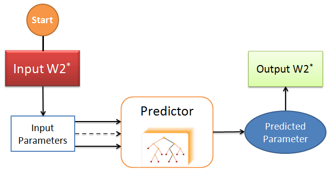


B.1 SDSS vs. WISE axial ratios and effective radii
One of the parameters that is involved in the calculation of dust extinction is , the average surface brightness of a galaxy in the W2 band within its effective radius (the radius that encloses half of the total light of that galaxy), corrected for the geometric effect of inclination. Here, is given by
| (B1) |
where and and are the semimajor and semiminor axes of the photometry aperture. The apparent effective surface brightness is calculated from
| (B2) |
where is the effective radius of the galaxy and W2 is its apparent magnitude. The value of depends on the W2-band magnitude, the axial ratio, and the half-light radius of the aperture used with the WISE images in the process of photometry.
The axial ratios of the apertures used for the photometry of SDSS and WISE images are plotted against each other in Fig. 37. The axial ratios of WISE apertures are systematically greater than the SDSS aperture axial ratios. In general, the morphology and visible size of a galaxy are different at optical and infrared wavelengths. Galaxy bulges are much more prominent at longer wavelengths. In addition, the point spread function (PSF) of WISE images is large compared to that of SDSS. Therefore, capturing all the galaxy light requires choosing larger axial ratios () when dealing with WISE images, where and are semi-major and semi-minor axes of the elliptical photometry apertures. In more face-on spirals ( approaching unity), the effects of bulges and PSF are less pronounced.
Galaxy effective radius is defined as the radius within which half of its total light is emitted. As an example, Fig. 38 plots the effective radius at the WISE W2 band against SDSS i band. We use linear models to describe the relation between the effective radii at optical g, r, i, and z bands and that at the W2 band. These relations are given as
| (B3) | ||||
| (B4) | ||||
| (B5) | ||||
| (B6) |
Bulges of spiral galaxies are more luminous at longer wavelengths because they are formed by red and dead stars. At longer wavelengths, we expect half-light radii to be smaller due to the centralized flux contributions of bulges. In Equation B6, this effect gives rise to larger coefficients at redward wave bands.
| No. | Output | rms | |||||||||
| % | % | % | % | % | % | % | % | % | mag | ||
| (1) | (2) | (3) | (4) | (5) | (6) | (7) | (8) | (9) | (10) | (11) | |
| 1 | 67.1 | 28.3 | 1.9 | 2.8 | 0.18 | ||||||
| 2 | 74.1 | 18.8 | 2.4 | 4.7 | 0.19 | ||||||
| 3 | 74.0 | 19.0 | 2.3 | 4.7 | 0.19 | ||||||
| 4 | 54.4 | 10.4 | 3.1 | 32.0 | 0.20 | ||||||
| 5 | 91.5 | 3.8 | 4.7 | 0.19 | |||||||
| 6 | 88.2 | 5.5 | 6.3 | 0.20 | |||||||
| 7 | 90.9 | 3.9 | 5.2 | 0.19 | |||||||
| 8 | 92.5 | 4.0 | 3.4 | 0.19 | |||||||
| 9 | 18.2 | 63.6 | 13.6 | 4.6 | 0.19 | ||||||
| 10 | 2.7 | 11.9 | 68.5 | 17.0 | 0.26 | ||||||
| 11 | 7.5 | 59.3 | 28.6 | 4.7 | 0.30 |
Note. Input parameters are denoted by their corresponding importance percentages. Column (11) tabulates the rms of , where is measured W2 and is the prediction of the algorithm displayed schematically in Fig. 40. In column (10), all color indices are in magnitude and is in mag arcsec-2.
B.2 Prediction Algorithm
Our goal here is to predict missing infrared W1 and W2 magnitudes. To begin, we need to establish a fiducial relation between distance-independent observables for a set of galaxies with both optical and infrared measurements. In Fig. 39, there is a plot of , the principal component parameter defined by Equation 4, versus , a color index corrected for host dust obscuration, for 2200 galaxies with both SDSS and WISE photometry. A linear relation describes this correlation and can be used to solve for given every other involved parameter. An optimal value for W2 can be found through testing a range of plausible values and adopting the value that forces the galaxy to obey the fiducial correlation.
Our algorithm, shown in Fig. 40, starts with an input guess value, for . The guess value along with other known parameters, such as optical magnitudes (presented in the form of optical-infrared colors), first principal component, H i line width, effective surface brightness at W2, etc., are then fed into the fiducial correlation, which outputs a parameter that is used to extract the parameter. Only one value of is consistent with the fiducial correlation (the input and output parameters agree with each other), and it is adopted as the predicted value of . Adopting the fiducial correlation illustrated in Fig. 39, we can derive over a range of and use these values to calculate the corresponding color indices. The output is then derived, given the i magnitude is known.
In Appendices B.3 and B.4, we use the random forest concept to explore a more complicated predictor and to incorporate a large number of galaxy features.


B.3 Random Forests
Random forest is a supervised machine-learning technique that uses training sets to capture the general trends in data and reach optimal performance in producing desired outputs. Normally, 80% of the data are used in the training process; these data are called the “training set”. Another 10% of the data are usually used to evaluate the algorithm performance and to optimize its structural hyperparameters in order to maximize its efficiency. This set is called the “cross validation set”. The remaining 10% of the data, called the “test set”, are held in reserve to evaluate the ultimate performance of the algorithm. These data are never used in the training and optimization process.
The building blocks of random forests are decision trees. Each decision tree in the forest is trained separately and is different from the other trees in the forest. The training of each tree can be randomized based on the following factors: (1) the number of input parameters and the order in which they are used for splitting and branching, and (2) the training of each tree being based on a randomly chosen subsample of the training set. The outputs of all random decision trees in the forest are averaged and reported as the ultimate output of the forest.
Decision trees are binary trees; their training is a recursive process and involves partitioning the training sample to maximize the information gain. At its root, each decision tree begins with the entire training sample. At each node, one of the input features is used to split the data set and pass it to the left and right children. The features and the splitting criteria are chosen to reach the largest possible information gain, given as
| (B7) |
where is the chosen feature that is used to perform the split, is the parent node dataset, and are the left and right children datasets, respectively. is the number of data points in each sample, and is the “Impurity Metric”, which is usually chosen to be the mean squared error (MSE). The MSE is the variance of the output feature, , in the sample
| (B8) |
where is the average of in the sample. The key to the machine-learning aspect of decision trees is that the machine decides how to split up the feature space at each node of the tree in order to minimize the cost criterion. The splitting at all nodes continues until reaching one of the training criteria. These criteria could be the maximum depth of the tree, the minimum number of data points at the leaf nodes, and/or a threshold on the increase of the information gain as the training advances. Intuitively, maximizing the information gain is equivalent to minimizing the total variance of the successive nodes. At the end of the training process, the leaf nodes contain data points whose target features, are almost analogous. MSE values closer to zero are better, as they indicate lower deviations of the predicted values from their true values.


B.4 Optimizations and Predictions
We use RandomForestRegressor from the Python package scikit-learn1414 14 https://scikit-learn.org/stable/modules/generated/sklearn.ensemble.RandomForestRegressor.html to train and evaluate our random forest models. A decision tree has a few parameters over which the user has control, called hyperparameters. Hyperparameters can be any internal parameters that control the training process, e.g. the number of levels in the tree (how deep the tree is) and how many leaves are allowed on each branch are two hyperparameters we set manually. The “cross-validation set” is used to optimize these parameters. Our optimized values for the maximum number of levels in trees and the minimum number of leaf galaxies are 14 and 9, respectively.
Figure 41 plots the differences between the measured and predicted values for three different sets, where the random forest was trained using the main principal component, , and , , and colors. The output parameter is chosen to be the color index. Each of the cross-validation and test sets contains 200 galaxies. The training set consists of 1800 galaxies. All of these sets are chosen randomly. The RMS scatter of differences between predicted and measured colors is 0.20 mag. The RMS scatter for the training set is slightly better, which indicates the possibility of overtraining the random forest.
In this study, input features and the output feature can be any of the distance-independent parameters introduced earlier. We attempt to understand which features are important in our best-fit model and which features are not as important. The importance of each feature is a function of (1) the number of nodes in the tree that use that particular feature and (2) the level of improvement in the ‘gain’ parameter. Those features that are used more frequently and contribute more in achieving more ‘gain’ are considered to be more important.
With the various parameters available, we attempt to find the combination of parameters that is optimal while including as much nonredundant information as possible. Some sets can achieve good results with fewer parameters, but they may force the algorithm to rely on a single parameter. The r and i bands have the smallest uncertainties, so the and outputs were expected to perform best. Table 5 shows a portion of the results. Each row of this table represents a random forest, the input features of which are indicated by the value of their importances, denoted as percentages. Column (10) lists the output parameter in each case. Column (11) tabulates the RMS scatter of the differences between measured and predicted W2 magnitudes in each case. Please refer to Appendix B.2 for more on how to derive W2 magnitudes. In practice, in the “Predictor” block of our algorithm (see Fig. 40), we use a trained random forest as an encoder that holds all the fiducial information determined to be useful in our problem.
Table 5 only lists the most promising combinations, and it tries to visit a variety of scenarios where one or a couple of magnitudes are missing due to poor image quality or other photometry problems. We find that the best performance is achieved when the output parameter is one of optical-infrared () colors. The input parameters are combinations of optical-optical colors and the first principal component, . For a given galaxy, we use all or a few of the random forest predictors and use their average predictions.
We explained our prediction algorithm in Appendix B.2. Instead of the simple linear fiducial correlation presented in Fig. 39, we use different random forest encoders presented in Table 5. We run the algorithm for a range of input values and end up with an output parameter. Fig. 42 plots the difference between input and output parameters, , as a function of the input parameter, for two galaxies taken from the test sample. The predicted value, , is at , where the input and output of the random forest model are in agreement with each other.
B.5 Evaluating the predicted parameters
The performance of our prediction method can be evaluated by comparing the predicted and measured parameters of the control sample (training and cross-validation sets). Fig. 43 plots the differences between predicted and measured values. In the top panel, the discrepancies are plotted against the measured values, . The 1 deviation of errors in the predicted values is mag. In the bottom panel, the deviations are plotted against the H i line widths that probe the absolute luminosity (and hence the size) of galaxies. No meaningful systematic is evident in either plot.
In the final part of the process, we use predicted W2 magnitudes, axial ratios, and effective radii to calculate the dust attenuation coefficient, (Equation 2). Uncertainties in predicted decrease with wavelength, ranging from 0.05 mag at g band to 0.01 mag at z band. As examples, Figures 44 and 45 plot the discrepancies between our predicted values of and the measured values versus various parameters. We observe no significant systematic correlations between discrepancies and the parameters used in these plots.

B.6 Evaluating the predicted parameters
In the previous section, we evaluated the performance of our method solely based on the OP+IR galaxies, meaning that the training and control galaxies have both optical and infrared data. Our tests show that our algorithm is capable of producing reasonable predictions that are in reasonable agreement with the measurements. However, we appreciate that the trained model is practically applied on spirals with missing infrared data. As discussed in Appendix A, the OPIR sample has different statistical characteristics than the OP+IR sample.
Figure 46 plots the main principal component, , versus line width, with the red and black points representing the OP+IR and OPIR galaxies, respectively. The values of the red points are calculated from measurement, whereas those of the black points are predictions of our algorithm. All predicted parameters seem to be smaller than the measured values. However, we attribute the offset to the average color difference of the two samples. Here, is the linear combination of line width, the color, and the average surface brightness at the W2 band (see Equation 4). As illustrated in the top panel of Figure 34, the OP+IR galaxies are slightly redder on average at a given line width. At a constant line width, redder spirals are formed by older stellar populations. They have a smaller ratio of H i to stellar mass, and hence their color index is larger (redder). Moreover, they are brighter at longer passbands, implying their to be smaller. These, together with the form of Equation 4 explain the differences between the average values of OP+IR and OPIR galaxies. In fact, the similarity between Figure 46 and the top panel of Figure 34 indirectly indicates that our predictive algorithm has successfully attained the essential aspects of our physical arrangement.
Appendix C On the calculations of uncertainties
In this work, multiple sources of uncertainties contribute to the final reported moduli uncertainties in Table 4:
- •
The uncertainty of the measured observable parameters that are directly used to calculate the galaxy distance modulus. These parameters are as follows: (1) apparent magnitudes of the galaxy at optical and infrared wave bands. (2) H i flux and line width, (3) galaxy spatial inclination, and (4) other geometrical features of the elliptical aperture that fits the galaxy.
The uncertainty of our measured magnitudes are no worse than mag at all wave bands except for the u band, where we adopt the conservative error of mag. To calculate the error of the surface brightness from Equations 5 and 6, in addition to the error of the measured apparent magnitudes, we considered an error of pixel (” for SDSS and ” for WISE) for the galaxy’s projected dimensions. We do not consider any error on the radial velocities of the galaxies because this parameter is never used in the determination of distances in this study. The uncertainties of all other parameters are reported in columns (3-37) of Table 1.
- •
The uncertainty in the fitted parameters of the applied relations. The main source of uncertainty is associated with the calibration of TFRs. The TFRs’ parameters and their uncertainties are listed in Table 2. We refer readers to K20 for a detailed discussion. The main concern regarding the TFRs is the vertical scatter of galaxies along the magnitude axis, which is larger than the statistical uncertainties we report for the measured distance moduli. Part of the scatter can be explained by the statistical uncertainties of the measured parameters that are involved in establishing TFRs (magnitudes and H i line widths), while there might be other contributions by some unknown physical processes that are not captured by the observables at our disposal. We list the RMS scatter about the TFR in Table 4. The covariances of the parameters of the fitted adjusting/regularizing relations in §III.3 and §III.4 are taken into account when they are employed to revise distance moduli.
- •
The uncertainty of the predicted quantities, for cases where a parameter is not directly available. In case of the predicted half-light radii and axial ratios, we combine the uncertainties of the dependent variable and uncertainties of the parameters of the fitted relations. The predicted dust attenuation depends on the estimated apparent magnitudes at the band. The RMS scatter of differences between measured and predicted values is 0.2 mag. The parameter is solely used to calculate , which is connected to through Equation 2. It is more reasonable to consider the scatter of differences between measured and predicted attenuation factors, . Similarly to what is presented in Figure 46, we determine respective scatters of 0.03 mag for and 0.02 mag for . Accordingly, we add these additional statistical scatters in quadrature to the error budget of the attenuation factors.
All the uncertainties in our calculations are accounted for following the Gaussian formalism of error propagation.
References
- Alam et al. (2015) Alam, S., Albareti, F. D., Allende Prieto, C., et al. 2015, ApJS, 219, 12, doi: 10.1088/0067-0049/219/1/12
- Bertin & Arnouts (1996) Bertin, E., & Arnouts, S. 1996, A&AS, 117, 393, doi: 10.1051/aas:1996164
- Courtois et al. (2009) Courtois, H. M., Tully, R. B., Fisher, J. R., et al. 2009, AJ, 138, 1938, doi: 10.1088/0004-6256/138/6/1938
- Courtois et al. (2011a) Courtois, H. M., Tully, R. B., & Héraudeau, P. 2011a, MNRAS, 415, 1935, doi: 10.1111/j.1365-2966.2011.18839.x
- Courtois et al. (2011b) Courtois, H. M., Tully, R. B., Makarov, D. I., et al. 2011b, MNRAS, 414, 2005, doi: 10.1111/j.1365-2966.2011.18515.x
- Fisher & Tully (1981) Fisher, J. R., & Tully, R. B. 1981, ApJS, 47, 139, doi: 10.1086/190755
- Freedman et al. (2019) Freedman, W. L., Madore, B. F., Hatt, D., et al. 2019, ApJ, 882, 34, doi: 10.3847/1538-4357/ab2f73
- Haynes et al. (2011) Haynes, M. P., Giovanelli, R., Martin, A. M., et al. 2011, AJ, 142, 170, doi: 10.1088/0004-6256/142/5/170
- Haynes et al. (2018) Haynes, M. P., Giovanelli, R., Kent, B. R., et al. 2018, ApJ, 861, 49, doi: 10.3847/1538-4357/aac956
- Hong et al. (2019) Hong, T., Staveley-Smith, L., Masters, K. L., et al. 2019, MNRAS, 487, 2061, doi: 10.1093/mnras/stz1413
- Huchtmeier & Richter (1989) Huchtmeier, W. K., & Richter, O. G. 1989, A General Catalog of HI Observations of Galaxies. The Reference Catalog. (Springer-Verlag New York)
- Jacob et al. (2010) Jacob, J. C., Katz, D. S., Berriman, G. B., et al. 2010, Montage: An Astronomical Image Mosaicking Toolkit. http://ascl.net/1010.036
- Joye & Mandel (2003) Joye, W. A., & Mandel, E. 2003, in Astronomical Society of the Pacific Conference Series, Vol. 295, Astronomical Data Analysis Software and Systems XII, ed. H. E. Payne, R. I. Jedrzejewski, & R. N. Hook, 489
- Kourkchi et al. (2020) Kourkchi, E., Tully, R. B., Anand, G. S., et al. 2020, The Astrophysical Journal, 896, 3, doi: 10.3847/1538-4357/ab901c
- Kourkchi et al. (2019) Kourkchi, E., Tully, R. B., Neill, J. D., et al. 2019, ApJ, 884, 82, doi: 10.3847/1538-4357/ab4192
- Krizhevsky et al. (2012) Krizhevsky, A., Sutskever, I., & Hinton, G. E. 2012, in Advances in Neural Information Processing Systems 25, ed. F. Pereira, C. J. C. Burges, L. Bottou, & K. Q. Weinberger (Curran Associates, Inc.), 1097–1105
- LeCun et al. (1998) LeCun, Y., Bottou, L., Bengio, Y., & Haffner, P. 1998, Proceedings of the IEEE, 86, 2278, doi: 10.1109/5.726791
- Magoulas et al. (2012) Magoulas, C., Springob, C. M., Colless, M., et al. 2012, MNRAS, 427, 245, doi: 10.1111/j.1365-2966.2012.21421.x
- Masci (2013) Masci, F. 2013, ICORE: Image Co-addition with Optional Resolution Enhancement. http://ascl.net/1302.010
- Masci & Fowler (2009) Masci, F. J., & Fowler, J. W. 2009, in Astronomical Society of the Pacific Conference Series, Vol. 411, Astronomical Data Analysis Software and Systems XVIII, ed. D. A. Bohlender, D. Durand, & P. Dowler, 67. https://arxiv.org/abs/0812.4310
- McGaugh et al. (2000) McGaugh, S. S., Schombert, J. M., Bothun, G. D., & de Blok, W. J. G. 2000, ApJ, 533, L99, doi: 10.1086/312628
- Neill et al. (2014) Neill, J. D., Seibert, M., Tully, R. B., et al. 2014, ApJ, 792, 129, doi: 10.1088/0004-637X/792/2/129
- Nelson et al. (2015) Nelson, D., Pillepich, A., Genel, S., et al. 2015, Astronomy and Computing, 13, 12, doi: 10.1016/j.ascom.2015.09.003
- Paturel et al. (2003) Paturel, G., Petit, C., Prugniel, P., et al. 2003, A&A, 412, 45, doi: 10.1051/0004-6361:20031411
- Riess et al. (2019) Riess, A. G., Casertano, S., Yuan, W., Macri, L. M., & Scolnic, D. 2019, ApJ, 876, 85, doi: 10.3847/1538-4357/ab1422
- Schechter (1976) Schechter, P. 1976, ApJ, 203, 297
- Sorce et al. (2014) Sorce, J. G., Tully, R. B., Courtois, H. M., et al. 2014, MNRAS, 444, 527, doi: 10.1093/mnras/stu1450
- Sorce et al. (2013) Sorce, J. G., Courtois, H. M., Tully, R. B., et al. 2013, ApJ, 765, 94, doi: 10.1088/0004-637X/765/2/94
- Springob et al. (2005) Springob, C. M., Haynes, M. P., Giovanelli, R., & Kent, B. R. 2005, ApJS, 160, 149, doi: 10.1086/431550
- Springob et al. (2007) Springob, C. M., Masters, K. L., Haynes, M. P., Giovanelli, R., & Marinoni, C. 2007, ApJS, 172, 599, doi: 10.1086/519527
- Springob et al. (2014) Springob, C. M., Magoulas, C., Colless, M., et al. 2014, MNRAS, 445, 2677, doi: 10.1093/mnras/stu1743
- Tully et al. (2016) Tully, R. B., Courtois, H. M., & Sorce, J. G. 2016, AJ, 152, 50, doi: 10.3847/0004-6256/152/2/50
- Tully & Fisher (1977) Tully, R. B., & Fisher, J. R. 1977, A&A, 54, 661
- Tully et al. (1996) Tully, R. B., Verheijen, M. A. W., Pierce, M. J., Huang, J.-S., & Wainscoat, R. J. 1996, AJ, 112, 2471, doi: 10.1086/118196
- Tully et al. (2013) Tully, R. B., Courtois, H. M., Dolphin, A. E., et al. 2013, AJ, 146, 86, doi: 10.1088/0004-6256/146/4/86
- Wright (2006) Wright, E. L. 2006, PASP, 118, 1711, doi: 10.1086/510102
- Wright et al. (2010) Wright, E. L., Eisenhardt, P. R. M., Mainzer, A. K., et al. 2010, AJ, 140, 1868, doi: 10.1088/0004-6256/140/6/1868
- York et al. (2000) York, D. G., Adelman, J., Anderson, Jr., J. E., et al. 2000, AJ, 120, 1579, doi: 10.1086/301513