The convexity of optimal transport-based waveform inversion for certain structured velocity modelsyunan.yang@nyu.edu
Courant Institute of Mathematical Sciences
New York, NY 10012-1185
Abstract
Full–waveform inversion (FWI) is a method used to determine properties of the Earth from information on the surface. We use the squared Wasserstein distance (squared distance) as an objective function to invert for the velocity of seismic waves as a function of position in the Earth, and we discuss its convexity with respect to the velocity parameter. In one dimension, we consider constant, piecewise increasing, and linearly increasing velocity models as a function of position, and we show the convexity of the squared distance with respect to the velocity parameter on the interval from zero to the true value of the velocity parameter when the source function is a probability measure. Furthermore, we consider a two–dimensional model where velocity is linearly increasing as a function of depth and prove the convexity of the squared distance in the velocity parameter on large regions containing the true value. We discuss the convexity of the squared distance compared with the convexity of the squared norm, and we discuss the relationship between frequency and convexity of these respective distances. We also discuss multiple approaches to optimal transport for non–probability measures by first converting the wave data into probability measures.
1 Introduction
The study of seismic waves has many practical applications in geology, especially in searching for natural resources such as oil or natural gas. It plays a major role in determining the type of material underground, given the position of several receivers on the surface and the amount of time it takes for the wave to rebound to the surface. The velocity of the wave (as a function of its position) is unknown, and finding the wave velocity function is equivalent to finding the underground substance. With the same wave source, different wave velocity properties produce different wave data (such as wave amplitude and travel time) measured at a given receiver. This wave data can be used to find the velocity. We use an objective function, or misfit function, which measures the “distance” between two sets of wave data. This allows us to compare the observed data with simulated data to find the true velocity function. Some examples of objective functions are the distance and the th Wasserstein distance ( distance) from the theory of optimal transport [20], the latter of which is the main tool of this research project.
The objective function becomes zero when the observed data and simulated data are equivalent, which occurs when we have the correct velocity model. Thus, finding the correct velocity model is an optimization problem: minimizing the objective function, which measures the error between simulated and observed wave data. Although it is necessary to have a gradient of zero to minimize the objective function, this is not enough, as it is possible to reach a saddle point or a local minimum at such a point. However, this issue is fixed if the objective function is convex, as it will have only one global minimum. Thus, it is important for the convex region near the global minimum to be as large as possible. For this reason, we investigate the convexity of the squared distance as an objective function.
The conventional choice of objective function is the least–squares norm, used in both time [19] and frequency [15, 16] domains. If we have data from multiple receiver locations (where is the index for the receiver location), we can consider the squared norm of the difference between the predicted wave data and the observed wave data
| (1.1) |
from [2], where is the true velocity parameter. While is minimized (and therefore equal to zero) exactly when algorithms for minimizing the squared norm may reach local minima instead of the global minimum when due to the nonconvexity of the squared norm as discussed in [2, 22]. In addition, its sensitivity to noise can make it an unsuitable choice of objective function [3]. Thus, we use the squared distance from [5, 22, 23] instead. If there are multiple receiver locations our final objective function will be
| (1.2) |
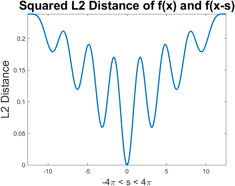
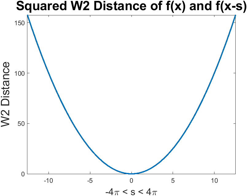
Previous results show that the squared metric is jointly convex in translations and dilations of the data [23], suggesting that the squared metric is a suitable choice for the objective function. Taking the function
as an example, we compare in Figure 1 the graphs of the squared norm of with the squared distance between and . It can be observed that the squared distance is convex in the shift while the graph of the squared norm is not.
In this paper, we present a theoretical approach to velocity inversion using optimal transport by investigating the convexity of the squared distance as a function of the velocity parameters – this has not been studied theoretically before. We investigate several velocity models in one dimension and show that the squared distance is a suitable objective function when inverting for the velocity parameter. In two dimensions, we consider a particular velocity model, and we show that the squared distance is a suitable objective function in the case where the source function is nonnegative. We generalize to when the source function alternates between negative and positive values, and we show that the squared distance is a suitable objective function given certain requirements on . These theorems suggest that the squared distance is a suitable objective function when is close enough to zero. Numerical evidence suggests that the squared distance is a better objective function than the squared norm when the source function is nonnegative.
The paper is structured as follows. In Section 2, we discuss background knowledge which is used later on in this paper. First, we introduce optimal transport and the distance, along with an explicit formula as well as some of its properties. Furthermore, we discuss the solution of wave equations in one dimension and introduce ray tracing, which is used to solve wave equations in higher dimensions. In Section 3, we first consider one–dimensional velocity models, where the velocity is either constant, piecewise constant, or linearly increasing as a function of position, and the source function is a probability measure. Then, we study a two–dimensional velocity model where the wave velocity satisfies where and are positive constants, is the horizontal position, and is the depth of the wave. Initially, in Section 3.3.1, we assume that the source function is a probability measure and that the wave amplitude is unchanged, and we show 4. In Section 3.3.2, we involve the wave amplitude and we allow the source function to alternate between positive and negative values, and we show 5. In Section 4, we compare the convexity of the squared distance with the squared norm, and we include numerical examples. We also discuss the relationship of the distance with the norm, and we discuss multiple approaches to optimal transport for non–probability measures. We summarize this paper in Section 5 and discuss a possible direction for future research.
2 Background
We introduce optimal transport, and essential background on wave equations.
2.1 Optimal Transport
In this section, we establish the main goal of optimal transport (originally introduced by Monge [14]) and introduce the distance along with some of its useful properties. Optimal transport involves probability spaces, which are nonnegative measure spaces with total measure equal to one. We discuss the convexity of the squared metric, which is a distance between two probability measures on a probability space, and introduce some of its properties.
2.1.1 General Problem

Consider two distinct probability measures and defined on the Borel sets of . The goal of optimal transport is to find a map , shown in Figure 2, which minimizes the total cost of mapping to according to the map for a given cost function [1]. The metric, based on optimal transport [24], gives the optimal transportation cost when the cost function is .
2.1.2 Computing the metric in one dimension
Let and be probability measures defined on the Borel sets of . We define the distance as
where , , is the support of , and is the set of all mass–preserving maps which map to . The integral within the infimum is the total cost of the transport map so computing is equivalent to minimizing the transport cost. We study the case where and our objective function is .
In one dimension, it is possible to express for probability measures and in a simpler way: Let and be the cumulative distribution functions of and respectively. Then, Rachev and Rüschendorf derive the formula for the squared distance in one dimension [17] as
| (2.1) |
where is the domain of . This formula for is useful when the wave data is only a function of time.
As wave data are not usually probability density functions, we can normalize a function defined on by replacing it with
for some constant such that for all [11].
2.1.3 Computing the Metric in Higher Dimensions
In general, there is no explicit formula to compute the metric in higher dimensions. However, certain requirements derived from the concept of cyclical monotonicity [13] make it possible to calculate the optimal map , and therefore the metric, through numerical methods. This is shown in the following theorem of Brenier [4, 6, 22]:
Theorem 1 (Brenier’s theorem).
Let and be two compactly supported probability measures on . If is absolutely continuous with respect to the Lebesgue measure, then there is a convex function such that the optimal map for the cost function is given by for –almost every .
Furthermore, if , then is differentiable –almost everywhere and
| (2.2) |
from the mass preserving property of . Replacing in Equation 2.2 with leads to the Monge–Ampère equation
where is the Hessian matrix of . Then, the squared distance satisfies
where is the domain of .
2.1.4 Properties of the Squared Distance
Results about the convexity of the squared distance with respect to changes in the data are known [9, 22, 23].
Theorem 2.
Let and be compactly supported probability density functions on an interval . Then,
| (2.3) |
where and is the optimal map from to . Furthermore, is convex in both and , for .
The convexity with respect to shifts and dilations suggests that the squared distance is more suitable when inverting for wave data.
2.2 Background on Wave Equation
We introduce the partial differential equation which governs the behavior of –dimensional waves. We also introduce d’Alembert’s solution to the one–dimensional wave equation and present the ray tracing approach to solving higher dimensional wave equations.
2.2.1 General Wave Equation
An –dimensional wave can be expressed as a function of position variables and time , which in general satisfies the partial differential equation
for a variable coefficient which is a function defined on , and a source function which is a function of both space and time. In general, the wave equation might not have an analytical solution.
2.2.2 Solution to 1D Wave Equation
In one dimension, we consider a simple case where is equal to a constant . The partial differential equation becomes
but unlike its –dimensional variant, it is possible to obtain an explicit solution as derived by d’Alembert [7]:
| (2.4) |
given the initial conditions and .
2.2.3 Solution for Higher Dimensional Wave Equation
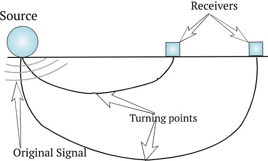
In higher dimensions, however, a wave equation might not have an analytical solution, so we use ray tracing to obtain information about the wave function [18]. An example of ray tracing is shown in Figure 3, where an original signal is released, and two receivers on the surface are present to measure the wave data. We assume that the velocity of a wave can be expressed as a function of depth in the Earth, and the ray parameter or the horizontal slowness, can be expressed as by Snell’s law where and is the angle the ray makes with a vertical axis. The ray parameter is constant throughout the path of the ray. We also define the vertical slowness as . The path of the ray is symmetric about a vertical line passing through a turning point at depth , and while . By examining a ray passing through several layers in the Earth and eventually returning to the surface, we may calculate the horizontal distance and the traveltime of the wave as a function of the velocity. We can calculate
| (2.5) |
as the distance from the source to the receiver, and
| (2.6) |
as the total travel time. Using Equation 2.5, it is possible to solve for in terms of and the velocity parameters. It is also possible to use Equation 2.6 to solve for as a function of and the velocity parameters, and it is possible to calculate the predicted time by guessing the velocity parameter. The method of traveltime tomography uses the above formulas to calculate the predicted time and approaches the problem as minimizing the squared difference between the predicted time and the observed time: [25].
However, this method does not work when the velocity model is not continuous [18]. In addition to using Equations 2.5 and 2.6, we make use of the wave’s amplitude as well to deal with discontinuous velocity models and other issues that traveltime tomography runs into. This method is known as full–waveform inversion (FWI), where both the amplitude and the traveltime are used to approximate the properties of the Earth [21].
The final amplitude is asymptotically scaled by a factor of
| (2.7) |
which is the reciprocal of the total arc length of the ray’s path [18], and the ray’s path is symmetric about the turning point at depth . Thus, if the source function is , then the observed wave function is approximated by . To invert for the velocity we use an objective function such as Equation 1.1 and Equation 1.2 to compare observed data with simulated data and minimize it using standard algorithms, and we will see that the squared metric can be a suitable choice.
3 Convexity in the Model Parameter
In this section, we study multiple velocity models in one dimension as well as a model in two dimensions, and we prove convexity of the squared distance with respect to the velocity parameter on certain domains. First, we consider one–dimensional velocity models. We begin with a model with constant velocity and prove convexity of the squared distance with respect to . We then consider two models with piecewise increasing velocities with respect to distance from the source and a model where velocity is linearly increasing. In every one–dimensional velocity model, we assume that the source function is nonnegative. Finally, we consider a two–dimensional model where the velocity satisfies where and are positive constants, is the horizontal position of the ray, and is the current depth of the ray. In Section 3.3.1, we assume that the source function is nonnegative, which allows us to use 2 when computing the squared distance. After this, we consider a more general case where the source function is alternating in Section 3.3.2, and the predicted wave function has an amplitude which is a function of , and the receiver location . We also use the following result [12]:
Lemma 1.
Let and be convex functions where and are convex sets and . Furthermore, assume is nondecreasing. Then, is a convex function on .
An example of this is when . Then, if is convex and nonnegative, we see that is also convex on its domain.
3.1 Constant Velocity in One Dimension
Let be the constant wave velocity, and let our initial wave function be . For this section, we assume that is a probability distribution. We assume that the final wave function at a fixed spatial location is of the form where is the amount of time it takes to receive the wave signals at location as a function of the velocity . Since the total distance is which means the predicted wave function is . Letting be the true value of the velocity gives us
as the squared distance from 2, because the integral in Equation 2.3 is zero. In addition, is a convex function of on and it is nonnegative on the interval . Hence, by 1, the squared distance is convex on .
Remark 1.
Due to the convexity of the squared distance in the interval , choosing a small value of as the initial guess guarantees being able to find the true velocity parameter through gradient–based optimization methods.
3.2 Non–constant Velocity in One Dimension
When the velocity is non–constant, the d’Alembert solution Equation 2.4 does not hold anymore. Thus, we study the convexity of the squared distance for several non–constant velocity models, shown in Figure 4. We first study a model where the velocity is piecewise constant, after which we add multiple pieces. Then, we study a model where the velocity is linearly increasing as a function of position. For all of these models, we assume that the source function is a probability distribution.


3.2.1 Piecewise Constant Velocity
The first scenario we study is a piecewise constant velocity model. Assume the velocity satisfies for and a known constant , and for , as seen in Figure 4(a) – we show convexity in the unknown . The total travel time, as a function of is . Letting be the true value of gives as the squared distance by 2. As the function is convex and nonnegative on the squared distance is also convex on by 1.
3.2.2 Piecewise Constant Velocity with Multiple Pieces
The second scenario we consider is the piecewise constant velocity with pieces of equal length such that the velocity of the wave is
Here, the unknown variable is . In this case, the total travel time is
so the squared distance becomes by 2 where is the true value of the velocity parameter. We claim that the squared distance is convex in on the interval . To do this, we initially show that is convex in on . Taking the second derivative, we get
which is nonnegative for all . Hence, is convex in on . Since is strictly decreasing on the function is nonnegative (and also convex) on the interval . Thus, the squared distance is convex in on the interval by 1.
3.2.3 Linearly Increasing Velocity
Next, we consider a linearly increasing velocity, which is of the form at a position for a known constant . Here, is unknown and is the true value of the velocity parameter. Letting be the total travel distance, we have the following integral representation for the traveltime:
| (3.1) |
We first prove a lemma.
Lemma 2.
is convex in on the interval , where .
Proof.
We take the second derivative of :
and the second equation follows by the Leibniz Integral Rule. Because , the integrand is nonnegative. This implies the convexity of . ∎
Now we are ready to show that is convex on the interval .
Theorem 3.
is convex in on the interval , where
Proof.
By 2, is convex. As the square of a nonnegative convex function is convex by 1, it is enough to determine the interval in which is nonnegative. From the integral representation of in Equation 3.1 we see that is strictly decreasing in . Hence, is nonnegative on the interval implying the convexity of on this interval by 1. ∎
3.3 A Velocity Model in Two Dimensions
Consider a velocity model in two dimensions where the predicted velocity at a point is of the form where and are positive constants, is the horizontal position of the ray, and is the current depth of the ray. We analyze the travel time of a ray emanating from a single receiver which has a final distance from the source, as well as the amplitude of the wave at a receiver. We compute the squared distance of the predicted wave function with the observed wave function (with velocity at depth ) and aim to find a region in for which this distance is convex in
3.3.1 Constant Amplitude
While the source function and the observed wave function always have the same amplitude in one dimension, for higher dimensions this is not the case. With a source function , the observed wave data is of the form for constants and because there are no reflections when the velocity is a continuous function of depth. However, we analyze the convexity with the assumption that . We treat the observed wave data as where is the predicted traveltime expressed as a function of and and is the observed traveltime of the wave data. is the receiver location, or the distance from the source to the receiver. Furthermore, we assume that is a probability distribution with compact support in the interval , where . When the source function is a probability distribution, this method is equivalent to traveltime tomography because the squared distance is equal to by 2.
Even when the observed wave data is not a probability distribution, we may normalize the data to reduce it to this case. For example, if we normalize a nonnegative function of the form with compact support in the interval using the formula , where is the normalized wave data, then the amplitude of the normalized data remains constant. Thus, the squared distance becomes .


Using this expression for the squared distance, we can determine its convexity in a large region containing and points arbitrarily close to the origin.
We first explicitly compute . Letting the ray parameter be we find that from Equation 2.5 where is the initial slowness, and is the initial vertical slowness. We can solve for and in terms of and as
From these formulas as well as Equation 2.6, we can solve for the time:
Then, the squared distance becomes where is the true velocity function. We first claim that is convex subject to a restriction on .
Lemma 3.
Let be the largest root of the equation , where
Then, the traveltime is jointly convex in whenever .
Proof.
Let and . We can compute the first order derivatives of as
The Hessian matrix of , where we treat as a constant, becomes , where
To prove the convexity of , it is enough to show that the Hessian matrix of is positive semidefinite, which is equivalent to showing that is positive semidefinite. Using Sylvester’s Criterion, because is always positive, we see that is positive semidefinite exactly when Letting
we see that
so it is enough to show that for all . Since is the largest root of , it is enough to show this inequality for all sufficiently large . Observe that for all sufficiently large , implying that which is at least for all sufficiently large . Since , this proves the lemma. ∎
We are now ready to prove the convexity of over a certain region .
Theorem 4.
Let and be positive constants, and let
where is a fixed constant. Then is nonempty and is jointly convex in .
Proof.
Remark 2.
To ensure that , it is enough to require that because is equal to . Thus, choosing large values of will ensure that the squared distance is convex in in a region containing . To find a suitable initial guess, we may choose a point such that and scale it by a sufficiently small constant in order to satisfy the condition .
However, this function is not suitable as an objective function because may equal its minimum, even when is not equal to or is not equal to – there is not enough information to find and through one receiver alone. To fix this, we add multiple receiver locations .
Fact 1.
The equation has at most one solution in where are fixed ordered pairs of positive real numbers.
Proof.
Assume for the sake of contradiction that the equation has two positive solutions. Since , there are at least three nonnegative solutions in to the equation . Therefore, the equation , or equivalently,
has at least two positive solutions in by the Mean Value Theorem. Thus, there are two positive solutions to the equation , a contradiction. ∎
This implies that the value of at two different receiver locations uniquely determines the pair . We use the objective function , where the sum is over the receivers , and the are the receiver locations. We plot this objective function in Figure 5(a), where and and the range from to inclusive. We compare it to the sum of the squared norm where the set of receiver locations is the same and the source function is . The –based objective function is mostly flat with a sharp incline close to the true velocity parameter . It is clearly nonconvex, as shown in Figure 5(b). On the other hand, the –based objective function (which does not depend on the source function, as long as it is nonnegative) appears convex in .
3.3.2 Varying Amplitude
In general, the amplitude of the wave equation solution is non–constant. The predicted wave function at receiver can be considered to be of the form
where is the amplitude as a function of the receiver location and the velocity parameters . The observed wave function at receiver can be considered of the form where is the true velocity parameter. Using Equation 2.7, we obtain
Since and are positive, we may simplify this expression to get
| (3.2) |
where
While the amplitude function in Equation 3.2 is not fully accurate, it is still a good approximation if the velocity model is continuous.
We will only consider points with and , which is a positive constant independent of . This also implies that . We treat as a sufficiently large constant, which causes to be large as well. In particular, is taken to be large enough so that . For large , the amplitude is approximately . Taking the derivative of the amplitude with respect to gives
Thus,
because . Similarly, because ,
Therefore, it is reasonable to assume the amplitude remains unchanged for large values of , and we let be this amplitude. We approximate a predicted wave function where is a fixed large constant by the new function so it suffices to approximate the observed wave function by the wave function .
As the distance is only defined when both of its inputs have total mass , we normalize all wave data of the form using the formula
on the interval and everywhere else. Here, is a positive constant such that for all .
Eventually, we compute the squared distance between and . We have
| (3.3) |
where , , and . We also assume that is large enough to ensure that and are strictly positive with total mass .
Then, we let
Since and are both probability distributions, we may compute the squared distance between them using Equation 2.1 to get
where is the unique function satisfying
for all and .
Observe that and can be expressed as functions of time and the velocity parameters , and can be expressed as a function of and . It is also possible to express as a function of and the predicted traveltime using Equation 3.3. Thus, we can alternatively express as a function of and , and as a function of and . In the proofs of the following claims, we sometimes omit the variables and in the arguments of and .
We compute to simplify .
Lemma 4.
Let , , and . Then, if ,
Proof.
From the substitution , we can compute as
We may write the integral as
However, note that As has compact support and , we may write the integral as . This becomes , where , and , which proves the lemma. ∎
Now, observe that the squared distance may be expressed as a function of , because is a function of both and . Using this, we may compute the first and second derivatives of with respect to . To compute the first derivative of with respect to , it is enough to find the first derivative of with respect to .
Lemma 5.
The first derivative of with respect to is
| (3.4) |
Proof.
Because we may apply the Leibniz integral rule to see that
Thus, we have that
From Equation 3.3, we see that
where we use the fact that . Thus, Equation 3.4 holds. ∎
Now, we use this to compute the first derivative of the squared distance with respect to .
Lemma 6.
Suppose . The first derivative of with respect to is
Proof.
Because ,
using the Leibniz integral rule. By 4 and 5 we simplify
From the change of variables , we see that , which can be computed as
This means
Furthermore, observe that from the substitution . Because is the inverse function of , we have that . Thus,
| (3.5) |
Observe that . From Equation 3.4, we have that
Substituting this expression for into Equation 3.5 gives
as the value of . ∎
Expressing in this form allows us to prove the convexity of with respect to subject to a restriction on the source function . Here, we assume that reaches both positive and negative values.
Theorem 5.
Let and suppose that . Let and be positive constants such that and let
Then, is nonempty and is jointly convex in .
Before beginning the proof of 5, we remark that the function with domain , where , and , satisfies the condition and reaches both positive and negative values. To see this, observe that while . Hence, our assumption that is a reasonable assumption to make.
Proof.
First, the point is clearly in , so is nonempty. Now, we prove that is jointly convex in . Because , is a subset of , which is defined in 4. This implies that is jointly convex in over the region by 3. Thus, it is enough to show that is convex and nondecreasing in in the interval . We first claim that is nondecreasing in in this interval. By 6, we see that
because . Furthermore, because , every factor is nonnegative, implying that is nonnegative. Next, we claim that is convex in in the interval . Using Equation 3.5 and 5, we see that
Since , we see that is nonnegative in the interval . Thus, is convex and nondecreasing in in the interval . Since is jointly convex in , is also jointly convex in by 1. ∎
Remark 3.
Through the Mean Value Theorem, 5 can be reformulated as a result with a condition involving an upper bound on . This reformulation illustrates how the convexity of is influenced by the frequency of the source function.
Remark 4.
The requirements needed to apply 1 are not satisfied for . To see this, observe that the squared distance is nonnegative everywhere and when . Thus, it is impossible for the squared distance to be nondecreasing in , although it may be convex in this interval.
4 Numerical Results
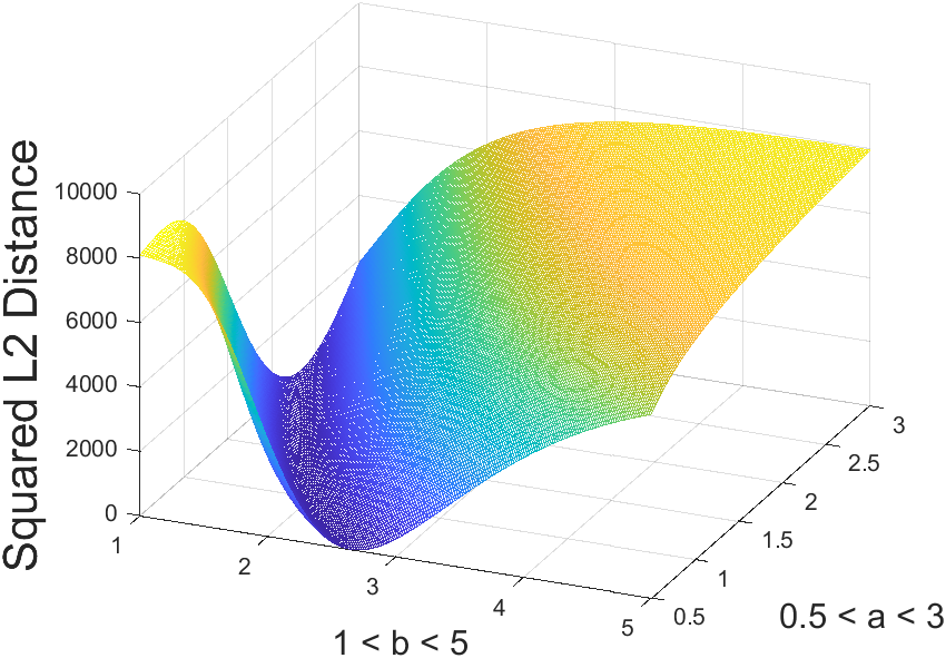


We continue with the velocity model studied in Section 3.3. We compute both the and distance and compare the convexity of the two objective functions in , as shown in Figures 6 and 7. The source wave function is of the form and we consider . Here, and . We can consider the observed data to be of the form because the velocity is a continuous function of the depth. To ensure that the wave data is compactly supported, we use the time range to compute the squared distance.
While the squared distance appears to be mostly convex for , the squared norm is certainly nonconvex. The plot of the squared norm has large flat regions with a steep incline closer to where the norm is minimized, as shown in Figures 6(a), 6(b) and 6(c). Although the squared norm is nonconvex, by decreasing the value of we increase the size of the convex region around of the squared norm. As the graph of the source function becomes sharper (Figure 9(a)), so does the graph of the squared norm. The squared distance, on the other hand, is relatively flat throughout the entire domain and does not have a steep incline closer to the minimum, as shown in Figures 7(a), 7(b) and 7(c). Thus, the squared distance should be convex on a much larger region containing the minimum. The squared distance is also highly insensitive to the choice of source function, and this suggests that the squared distance can be used to solve various seismic inversion problems, in contrast with the squared norm.
In addition, we plot the sum of the squared distance taken over multiple receiver locations in Figure 8. The summation of the squared distance over multiple receiver locations is highly convex regardless of , as seen in Figures 8(a), 8(b) and 8(c). Furthermore, the summation of the squared distance over multiple receiver locations is also very close to the summation of over multiple receiver locations, and appears to be convex in for closer to the origin. Thus, as an initial guess for , it appears to be better to choose points which are very close to the origin. This is equivalent to choosing points such that the predicted travel time is large.
4.1 Frequency Analysis
We observe that the changes in the squared or distances between and depends solely on the value of , which in turn affects the frequency of the source function. The graph of the source function in the frequency domain can be derived by taking a Fourier transform. Letting
we get that , and the power at a frequency is given by the magnitude, which is . The graph of is centered at regardless of the value of , but as the value of increases, the plot of becomes wider, as shown in Figure 9(b). In other words, if where and are fixed frequencies, then increases as increases. Thus, as the value of increases, the average absolute value of the frequency of the source function also increases. For large values of , the plot of the squared norm also has the properties of higher frequency data, as the plot is very sharp close to . The high–frequency data seen in Figure 6(c) is explained by the squared norm weighting low–frequency and high–frequency terms equally, by the Plancherel Theorem. On the other hand, the plot of the squared distance is virtually unchanged as increases, suggesting that the frequency of the the squared distance is highly insensitive to the frequency of the source function.
The relationship between the distance between two functions and and a weighted distance between them helps provide an explanation for these observations regarding frequency [10, 20]. We define the space through the seminorm
and the space is defined as the dual of through the norm
It is known [20] that the distance is asymptotically equivalent to the norm, which weights terms of lower frequency over terms with higher frequency. Specifically, if is a probability measure and is an infinitesimal perturbation with zero total mass, then [10]. While the objective functions in Figures 7 and 8 are not globally convex, the relationship between the squared distance and the squared metric offers an explanation for the smoothness of the plots in these figures, which display properties of low–frequency data.
4.2 Optimal Transport for Non–probability Measures
In general, the wave data tends to alternate between positive and negative values, and the total integral of the observed or predicted wave function does not have to be . Thus, we cannot immediately use the squared distance as our objective function, because it is only defined on probability distributions. The current approach to normalizing the wave data requires two steps: first, transform the wave data to a nonnegative function, and second, divide by the total mass [8]. This ensures that the normalized wave data satisfies the positivity and total mass requirements. Although there are several possible ways to complete the first step, the known methods of doing this have their own drawbacks.
If the source function is positive, the first step becomes unnecessary. The requirement in 4 is not very strong, suggesting that when is positive, the squared distance is suitable as an objective function. However, this method does not generalize well to source functions that alternate between negative and positive values. In this case, we complete the first step by initially replacing an alternating function by , where . Then, we divide by the total mass of in the interval . This method of normalization takes into account the wave amplitude as well. However, the convexity of the squared distance, in this case, is not as general as with the previous method. Further restrictions on the source are necessary, as shown by the requirements in 5. This suggests that the squared distance is suitable as an objective function when the normalization constant is sufficiently close to , or equivalently, when is sufficiently close to .
5 Conclusions
In this paper, we study the convexity of full–waveform inversion using the squared distance as an objective function with respect to the velocity model parameter. We show that the squared distance is a suitable objective function for multiple velocity models when the received signal is nonnegative. Next, we show that the squared distance is suitable in some cases, in a two–dimensional velocity model where the received signal alternates between positive and negative values. We review the smoothing property of the squared distance by its relation to the squared distance, and contrast this with the sharpness of the squared norm, which is very sensitive to high–frequency signals. We also discuss the drawbacks of the normalization methods used in this paper. A natural direction for future research is to generalize the distance to compare functions alternating between positive and negative values.
6 Acknowledgements
Firstly, the author would like to thank Dr. Yunan Yang for her mentorship and guidance during this project. The author thanks Dr. Tanya Khovanova and Boya Song for proofreading this paper and for providing feedback. Finally, the author is thankful to the PRIMES–USA program for making this research project possible. This work is supported in part by the National Science Foundation through grant DMS–1913129.
References
- [1] Luigi Ambrosio and Nicola Gigli. A user’s guide to optimal transport. In Modelling and optimisation of flows on networks, pages 1–155. Springer, 2013.
- [2] Hyoungsu Baek, Henri Calandra, and Laurent Demanet. Velocity estimation via registration-guided least-squares inversion. Geophysics, 79(2):R79–R89, 2014.
- [3] Ebru Bozdağ, Jeannot Trampert, and Jeroen Tromp. Misfit functions for full waveform inversion based on instantaneous phase and envelope measurements. Geophysical Journal International, 185(2):845–870, 2011.
- [4] Yann Brenier. Polar factorization and monotone rearrangement of vector-valued functions. Communications on pure and applied mathematics, 44(4):375–417, 1991.
- [5] Jing Chen, Yifan Chen, Hao Wu, and Dinghui Yang. The quadratic Wasserstein metric for earthquake location. Journal of Computational Physics, 373:188–209, 2018.
- [6] Guido De Philippis and Alessio Figalli. The Monge–Ampère equation and its link to optimal transportation. Bulletin of the American Mathematical Society, 51(4):527–580, 2014.
- [7] Laurent Demanet. Waves and imaging class notes-18.325, 2016.
- [8] Björn Engquist and Brittany D. Froese. Application of the Wasserstein metric to seismic signals. arXiv preprint arXiv:1311.4581, 2013.
- [9] Björn Engquist, Brittany D. Froese, and Yunan Yang. Optimal transport for seismic full waveform inversion. arXiv preprint arXiv:1602.01540, 2016.
- [10] Björn Engquist, Kui Ren, and Yunan Yang. The quadratic Wasserstein metric for inverse data matching. Inverse Problems, 36(5):055001, 2020.
- [11] Björn Engquist and Yunan Yang. Seismic imaging and optimal transport. arXiv preprint arXiv:1808.04801, 2018.
- [12] Ayman Hourieh. The composition of two convex functions is convex. Mathematics Stack Exchange. URL:https://math.stackexchange.com/q/287725 (version: 2013-01-26).
- [13] Martin Knott and Cyril S. Smith. On the optimal mapping of distributions. Journal of Optimization Theory and Applications, 43(1):39–49, 1984.
- [14] Gaspard Monge. Mémoire sur la théorie des déblais et des remblais. Histoire de l’Académie Royale des Sciences de Paris, 1781.
- [15] R. Gerhard Pratt. Inverse theory applied to multi-source cross-hole tomography.: Part 2: Elastic wave-equation method1. Geophysical Prospecting, 38(3):311–329, 1990.
- [16] R. Gerhard Pratt and Michael H. Worthington. Inverse theory applied to multi-source cross-hole tomography. part 1: Acoustic wave-equation method 1. Geophysical prospecting, 38(3):287–310, 1990.
- [17] Svetlozar T. Rachev and Ludger Rüschendorf. Mass Transportation Problems: Volume I: Theory, volume 1. Springer Science & Business Media, 1998.
- [18] Peter M. Shearer. Introduction to seismology. Cambridge university press, 2019.
- [19] Albert Tarantola. Inverse problem theory and methods for model parameter estimation. SIAM, 2005.
- [20] Cédric Villani. Topics in optimal transportation. American Mathematical Soc., 2003.
- [21] Jean Virieux and Stéphane Operto. An overview of full-waveform inversion in exploration geophysics. Geophysics, 74(6):WCC1–WCC26, 2009.
- [22] Yunan Yang. Optimal transport for seismic inverse problems. PhD thesis, The University of Texas at Austin, 2018.
- [23] Yunan Yang. Analysis and application of optimal transport for challenging seismic inverse problems. arXiv preprint arXiv:1902.01226, 2019.
- [24] Yunan Yang and Björn Engquist. Analysis of optimal transport and related misfit functions in full-waveform inversion. Geophysics, 83(1):A7–A12, 2018.
- [25] Colin A. Zelt. Traveltime tomography using controlled-source seismic data. Encyclopedia of solid earth geophysics, 2:1453–1473, 2011.