An overlapping local projection stabilization for Galerkin approximations of Darcy and Stokes problems

Deepika Garg Email: deepika.lpu.pbi@gmail.com, deepikagarg@iisc.ac.in Address: National Mathematics Initiative, Indian Institute of Science, Bangalore - 560012, India Sashikumaar Ganesan Email: sashi@iisc.ac.in Address: National Mathematics Initiative, Indian Institute of Science, Bangalore - 560012, India Address: Department of Computational and Data Sciences, Indian Institute of Science, Bangalore - 560012, India

August 11, 2026

Abstract

A priori analysis for a generalized local projection stabilized conforming finite element approximation of Darcy flow and Stokes problems is presented in this paper. A first-order conforming $\mathbf{P}^{c}_{1}$ finite element space is used to approximate both the velocity and the pressure. It is shown that the stabilized discrete bilinear form satisfy the inf-sup condition with respect to a generalized local projection norm. Moreover, a priori error estimates are derived for both problems. Finally, the validation of the proposed stabilization scheme is demonstrated with appropriate numerical examples.

Key words: Finite element method; Darcy flows; Stokes problem; Generalized local projection stabilization; Stability; Inf-sup condition; Error estimates.

AMS subject classification: 65N30, 65N15, 65N12, 76M10.

1 Introduction

The numerical solution of Darcy equations has considerable practical importance in civil, petroleum, and electrical engineering, such as flow in porous media, heat transfer, semiconductor devices, etc. In general, numerical schemes for Darcy equations can be divided into two categories: (i) primal, a single-field formulation for pressure, and (ii) mixed two-field formulation in which pressure and velocity are variables.

Eliminate the velocity from mixed two-field formulation results in a scalar second-order partial differential equation ( PDEs) for the pressure. The construction of finite element methods based on this kind of formulation is straightforward. However, this direct approach results in lower-order velocity approximations compared to the pressure. Alternative approaches such as mixed methods [15] and post-processing techniques [36] have been used to improve the approximation of the velocity. The mixed finite element method based on the Galerkin formulation has increasingly become popular to discretize the Darcy equations. The classical mixed variational formulation of Darcy equations is posed in the Sobolev spaces $\rm{H}(\mbox{div},\Omega)\ \text{and}\ {\rm{L}^{2}_{0}(\Omega)}$ for the velocity and pressure, respectively. It has been a challenge to develop finite dimensional subspaces of these spaces that satisfy the inf-sup stability condition. Indeed, the choice of interpolation spaces is restricted when imposing this inf-sup stability condition. Nevertheless, a few finite element pairs that satisfy the inf-sup condition has been proposed. The well-known successful combinations are the Raviart-Thomas [39] and the Brezzi-Douglas-Marini [14], which requires the continuity of normal component of the velocity in combination with specific discontinuous pressure interpolation. However, such choices result in saddle point problems, which are more challenging to solve.

In this study, we propose a mixed finite element formulation with a generalized local projection stabilized conforming finite element method for Darcy equations, which avoids ${\rm H}(\mbox{div},\Omega)$ approximation space. It is well-known that the application of standard Galerkin finite element method (FEM) to the Darcy equations induces spurious oscillations in the numerical solution. Nevertheless, the stability and accuracy of the standard Galerkin solution can be enhanced by applying a stabilization technique. Several stabilization methods such as streamline diffusion methods [40, 41], least-square methods [1, 11, 32], residual-free bubbles [1, 16, 27], local projection schemes [9, 23, 28, 29, 38], continuous interior penalty methods [17, 18, 19, 20] and many more have been proposed in the literature. The basic idea of stabilization is to stabilize the Galerkin variational formulation so that the discrete approximation is stable and convergent; see, for example, [6, 5, 18, 21, 22, 37]. Stabilization methods for Stokes-like operators are well-studied in the literature, see for example [3, 28] and a few studies for Darcy equations have also been presented, see for example [6, 5, 37, 38].

The local projection stabilization (LPS) method has been proposed in [3, 9] for the Stokes problem and subsequently extended to various other classes of problems [8, 28, 29, 31, 35, 38]. The LPS is based on a projection of the finite element space $Y_{h}$ , which approximates the unknown to the discontinuous space $D_{h}$ , see [3, 9]. LPS is very attractive, mainly because of its commutation properties in optimization problems [7] and similar stabilization properties to those of residual approaches [34]. A significant benefit of the local projection method is that the LPS approach uses a symmetric stabilization term and contains fewer stabilization terms than the residual-based stabilization approach. Generalized local projection stabilization (GLPS) is a more generalized form of LPS that allows us to define local projection spaces on overlapping sets. GLPS has first been introduced and studied for the convection-diffusion problem in [25, 33] and for the Oseen problem in [4, 35], recently, for the advection-reaction equations in [30]. A priori analysis in [33, 35] is based on an inf-sup condition for $Y_{h}$ and $D_{h}$ spaces and the existence of orthogonal projection of $Y_{h}$ into $D_{h}$ . Further, unlike LPS, GLPS needs neither a macro grid nor an enrichment of approximation spaces.

The main contributions of this paper are the development of a GLPS conforming finite element scheme for Darcy equations and the derivation of its stability and convergence estimates. In the present analysis, we approximate the velocity and pressure with the piecewise linear polynomial finite element space. In particular, the use of piecewise linear finite elements for both the velocities and the pressure results in ill-posed discretizations. Therefore, GLPS is proposed in this work to suppress the oscillations in the approximations. The boundary conditions are not used strongly in discrete space; hence, the discrete formulation is a combination of standard Galerkin formulations, stabilization terms, and weakly imposed boundary conditions. The proposed bilinear form satisfies an inf-sup condition with respect to generalized local projection stabilized norm, which leads to the well-posedness of the discrete problem. A priori error analysis assures the optimal order of convergence, that is, $\mathcal{O}(h^{3/2})$ in the case of $(\mathbf{P}^{c}_{1}/\mathbf{P}^{c}_{1})$ conforming finite element approximation. Furthermore, the above approach has also been used to study the Stokes problem. We give an elementary proof of stability and convergence analysis for the Stokes problem.

The outline of the article is as follows: In Section 2, we introduce the weak formulation of the Darcy flow, notations, and preliminaries, which are used throughout the paper. Section 3.1 is devoted to an overlapping local projection stabilized conforming finite element methods in which we derive the stability analysis with respect to a generalized local projection norm. In section 3.2, we provide an optimal a priori error estimates with respect to a generalized local projection norm. In Section 4, we extended the above result to Stokes problem in the conforming FEM. Section 5 presents some numerical experiments that confirm the theoretical analysis.

2 The Darcy problem

Let $\Omega\subset\mathbb{R}^{2}$ be an open bounded polygonal domain with smooth boundary $\partial{\Omega}$ . Consider the following Darcy flow equations: Find $(\textbf{u},p)$ such that

	$\displaystyle\textbf{u}+\nabla p=\textbf{f};\quad\nabla\cdot\textbf{u}$	$\displaystyle=\phi\ \ \text{\ in}\ \Omega,$		(1)
	$\displaystyle\textbf{u}\cdot\textbf{n}$	$\displaystyle=0\ \ \text{ on}\ \partial{\Omega}.$

Here, u denotes the velocity vector, $p$ is the pressure, $\textbf{f}\in[\rm{L}^{2}(\Omega)]^{2}$ is the source function, $\phi$ is the volumetric flow rate source, and n is the unit outward normal vector to $\partial{\Omega}$ . The divergence constraint implies that the prescribed data must satisfy the condition

\displaystyle\int_{\Omega}\phi\;\textit{dx}=0.

In order to formulate a weak formulation of the Darcy flow equations, we consider the following Sobolev spaces

\textbf{V}:=\left\{\textbf{v}\in\rm{H}(\mbox{div},\Omega)|\ \textbf{v}\cdot\textbf{n}=0\ \text{on}\ \partial{\Omega}\right\},\quad Q:=\rm{L}^{2}_{0}(\Omega)=\left\{q\in\rm{L}^{2}(\Omega)|\ \int_{\Omega}{q}\;\textit{dx}=0\ \right\},

where $\rm{L}^{2}(\Omega)$ is a space of square-integrable measurable function. Moreover, a weak formulation of the model problem (1) reads: Find $(\textbf{u},p)$ $\in\textbf{V}\times Q$ such that

a(\textbf{u},\textbf{v})-b(p,\textbf{v})=(\textbf{f},\textbf{v});\qquad b(\textbf{u},q)=(\phi,q),

for all $v\in\textbf{V}$ and $q\in Q$ . Here, $(\cdot,\cdot)$ denotes the $\rm{L}^{2}(\Omega)$ inner product and

\displaystyle a(\textbf{u},\textbf{v}):=\int_{\Omega}{\textbf{u}\cdot\textbf{v}}\;\textit{dx};\ \ \ b(p,\textbf{v}):=\int_{\Omega}p\nabla\cdot\textbf{v}\;\textit{dx}.

An equivalent weak formulation of the model problem can be defined on the product space $\textbf{V}\times Q$ and it reads: Find $(\textbf{u},p)\ \in\textbf{V}\times Q\text{ such that }$

A((\textbf{u},p),(\textbf{v},q))=L(\textbf{v}),

(2)

for all $(\textbf{v},q)\in\textbf{V}\times Q$ , where

A((\textbf{u},p),(\textbf{v},q)):=a(\textbf{u},\textbf{v})-b(p,\textbf{v})+b(q,\textbf{u});\qquad L(\textbf{v}):=(\textbf{f},\textbf{v})+(\phi,q).

Furthermore, Banach-Ne $\check{c}$ as-Babu $\check{s}$ ka theorem [26, pp. 85] guarantees that the model problem (1) is well-posed in $\textbf{V}\times Q$ , for more details; see [26, pp. 230].

2.1 Finite element formulation

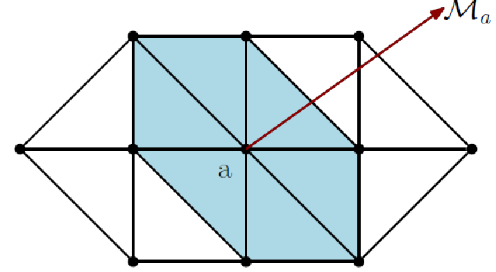
Let $\mathcal{T}_{h}$ be a collection of non-overlapping quasi-uniform triangles obtained by a decomposition of $\Omega$ . Let $h_{K}=\rm{diam}(K)$ for all $K\in\mathcal{T}_{h}$ and the mesh-size $h=\mbox{max}_{K\in\mathcal{T}_{h}}h_{K}$ . Let $\mathcal{E}_{h}=\mathcal{E}_{h}^{I}\cup\mathcal{E}_{h}^{B}$ be the set of all edges in $\mathcal{T}_{h}$ , where $\mathcal{E}_{h}^{I}$ and $\mathcal{E}_{h}^{B}$ are the set of all interior and boundary edges, respectively, and $h_{E}=\rm{diam}(E)$ for all $E\in\mathcal{E}_{h}$ . Let $\mathcal{V}_{h}:=\mathcal{V}_{h}^{I}\cup\mathcal{V}_{h}^{B}$ be the set of all vertices in $\mathcal{V}_{h}$ , where $\mathcal{V}_{h}^{I}$ and $\mathcal{V}_{h}^{B}$ are the set of all interior and boundary vertices, respectively. For any $a\in\mathcal{V}_{h}$ , we denote by ${\mathcal{M}}_{a}$ (patch of $a$ ) the union of all cells that share the vertex $a$ . Further, define $h_{a}=\rm{diam}(\mathcal{M}_{a})$ for all $a\in\mathcal{V}_{h}$ . Moreover, We use the following norm in the analysis. Let the piecewise constant function $h_{\mathcal{T}}$ is defined by $h_{\mathcal{T}}|_{K}=h_{K}$ and $s\in\mathbb{R}$ and $k\geq 0$

\displaystyle\left\|h_{\mathcal{T}}^{s}u\right\|_{k}=\left(\sum_{K\in\mathcal{T}_{h}}h_{K}^{2s}\left\|u\right\|^{2}_{\rm{H}^{k}(K)}\right)^{\frac{1}{2}}\text{ for all}\ u\in\ \rm{H}^{k}(\mathcal{T}_{h}).

Refer to caption — Figure 1: Node patch ${\mathcal{M}}_{a}$ .

Suppose $I(a)$ denotes the index set for all $K_{l}$ elements, so that $K_{l}\subset{\mathcal{M}}a$ . Then, the local mesh-size associated to ${\mathcal{M}}_{a}$ is defined as

\displaystyle{h}_{a}:=\frac{1}{\mbox{card}(I(a))}\sum_{l\in I(a)}h_{l},\quad\text{ for each}\ a\in\mathcal{V}_{h},

where $\text{card}(I(a))$ denotes the number of elements in ${\mathcal{M}}_{a}$ . Since the mesh $\mathcal{T}_{h}$ is assumed to be locally quasi-uniform [10], there exists a positive $\zeta\geq 1$ independent of $h$ such that

\displaystyle\zeta^{-1}\leq\frac{{h}_{a}}{h_{l}}\leq\zeta\text{ for all}\ l\in I(a).

For any $a\in\mathcal{V}_{h}$ , define the fluctuation operator $\kappa_{a}:\rm{L}^{2}(\mathcal{M}_{a})\rightarrow\rm{L}^{2}(\mathcal{M}_{a})$ by

\displaystyle\kappa_{a}(v)=v-\frac{1}{|\mathcal{M}_{a}|}\int_{\mathcal{M}_{a}}v\;\textit{dx}.

We next define a piecewise polynomial space as

\displaystyle\mathbb{P}_{k}(\mathcal{T}_{h}):=\left\{v\in\rm{L}^{2}(\Omega):v|_{K}\in\mathbb{P}_{k}(K)\quad\forall K\in\mathcal{T}_{h}\right\},

where $\mathbb{P}_{k}(K)$ , $k\geq 0$ , is the space of polynomials of degree at most $k$ over the element $K$ . Further, define a conforming finite element space of piecewise linear

\displaystyle\mathbf{P}^{c}_{1}(\mathcal{T}_{h}):=\left\{v\in\rm{H}^{1}(\Omega)\ :\ v|_{K}\in\mathbb{P}_{1}(K)~~\forall~K\in\mathcal{T}_{h}\right\}.

Now recall the following technical results of finite element analysis.

Lemma 2.1

Trace inequality [24, pp. 27]: Suppose E denotes an edge of $K\in\mathcal{T}_{h}$ . For $v_{h}\in\mathbb{P}_{k}(\mathcal{T}_{h})$ , there holds

\displaystyle\|v_{h}\|_{\rm{L}^{2}(E)}

\displaystyle\leq Ch_{K}^{-1/2}\|v_{h}\|_{\rm{L}^{2}(K)}.

(3)

Lemma 2.2

Inverse inequality [24, pp. 26]: Let $v\in\mathbb{P}_{k}(\mathcal{T}_{h})$ , for all $k\geq 0$ ; then

\displaystyle\left\|\nabla{v}\right\|_{K}\leq Ch^{-1}_{K}\left\|v\right\|_{K}.

(4)

Lemma 2.3

Poincaré inequality [12, pp. 104]: For a bounded and connected polygonal domain ${\Omega}$ and for any $v\in\rm{H}^{1}({\Omega})$ , we have

\displaystyle\left\|v-\frac{1}{|{\Omega}|}\int_{{\Omega}}v\;\textit{dx}\right\|_{\rm{L}^{2}({\Omega})}\leq Ch_{\Omega}\left\|\nabla v\right\|_{\rm{L}^{2}({\Omega})},

where $h_{\Omega}$ and $|{\Omega}|$ denote the diameter and the measure of domain ${\Omega}$ . In particular, for every vertex $a\in\mathcal{V}_{h}$ and every function $v\in\rm{H}^{1}({\mathcal{M}_{a}})$ , it holds

\displaystyle\left\|v-\frac{1}{|{\mathcal{M}}_{a}|}\int_{{\mathcal{M}}_{a}}v\;\textit{dx}\right\|_{\rm{L}^{2}({\mathcal{M}}_{a})}\leq Ch_{a}\left\|\nabla v\right\|_{\rm{L}^{2}({\mathcal{M}}_{a})},

(5)

where the constant $C$ is independent of the mesh-size $h_{a}$ .

Furthermore, for a locally quasi-uniform and shape-regular triangulation the $\rm{L}^{2}$ -orthogonal projection $I_{h}:\rm{L}^{2}(\Omega)\rightarrow\mathbf{P}_{1}^{c}(\mathcal{T}_{h})$ satisfies the following approximation properties, for more details; see [2, 25].

Lemma 2.4

$\rm{L}^{2}$ -Orthogonal projections: The $\rm{L}^{2}$ -projection $I_{h}:\rm{L}^{2}(\Omega)\rightarrow\mathbf{P}^{c}_{1}(\mathcal{T}_{h})$ satisfies

\displaystyle\left\|h_{\mathcal{T}}^{-1}({v-I_{h}v})\right\|+\left\|\nabla(v-I_{h}v)\right\|

\displaystyle\leq C\left\|h_{\mathcal{T}}v\right\|_{2},\ {\rm for~all}\ v\in\rm{H}^{2}(\Omega),

(6)

For vector valued functions $\mathbf{I}_{h}:[\rm{L}^{2}(\Omega)]^{2}\rightarrow[\mathbf{P}^{c}_{1}(\mathcal{T}_{h})]^{2}$ satisfy

\displaystyle\left\|h_{\mathcal{T}}^{-1}({\mathbf{v}-\mathbf{I}_{h}\mathbf{v}})\right\|+\left\|\nabla(\mathbf{v}-\mathbf{I}_{h}\mathbf{v})\right\|

\displaystyle\leq C\left\|h_{\mathcal{T}}\mathbf{v}\right\|_{2}\ {\rm for~all}~\mathbf{v}\in[\rm{H}^{2}(\Omega)]^{2}.

(7)

Moreover, the trace inequality over each edge imply

\displaystyle\left(\sum_{E\in\mathcal{E}_{h}}\left\|\mathbf{v}-\mathbf{I}_{h}\mathbf{v}\right\|^{2}_{\rm{L}^{2}(E)}\right)^{1/2}

\displaystyle\leq C\left\|h_{\mathcal{T}}^{3/2}\mathbf{v}\right\|_{2}\ {\rm for~all}~~\mathbf{v}\in[\rm{H}^{2}(\Omega)]^{2}.

(8)

The orthogonality relation for all $\mathbf{v}_{h}\in[\mathbf{P}^{c}_{1}(\mathcal{T}_{h})]^{2}$ imply

\displaystyle(\mathbf{v}-\mathbf{I}_{h}\mathbf{v},\mathbf{v}_{h})_{\rm{L}^{2}(\Omega)}=0,

(9)

The following approximation estimates hold for the $L^{2}$ -orthogonal projection operator

\left\|\mathbf{I}_{h}\mathbf{v}\right\|\leq\left\|\mathbf{v}\right\|,\quad\left\|h^{-1}_{\mathcal{T}}\mathbf{I}_{h}\mathbf{v}\right\|\leq C\left\|h^{-1}_{\mathcal{T}}\mathbf{v}\right\|,\quad\left\|\nabla(\mathbf{I}_{h}{v})\right\|\leq C\left\|\nabla{\mathbf{v}}\right\|.

(10)

Note that throughout this paper, C (sometimes subscripted) denotes a generic positive constant, which may depend on the shape-regularity of the triangulation but is independent of the mesh-size. Further, the notation $c\lesssim d$ represents the inequality $c\leq Cd$ . Moreover, $(\cdot,\cdot)$ represents the $\rm{L}^{2}(\Omega)$ inner product; and $\rm{L}^{2}(\Omega)$ and $\rm{L}^{\infty}(\Omega)$ norms are respectively denoted by $\left\|u\right\|$ and $\left\|u\right\|_{\infty}$ . The standard notation of Sobolev space $\rm{H}^{s}(\Omega),$ for s=1,2 and its norm $\left\|\cdot\right\|_{r}$ respectively, are used. The notation $[\rm{L}^{2}(\Omega)]^{2}$ and $[\rm{H}^{1}(\Omega)]^{2},$ respectively, abbreviates the vector-valued version of $\rm{L}^{2}(\Omega)$ and $\rm{H}^{1}(\Omega)$ and $\rm{H}_{0}^{1}(\Omega)$ is a subspace of $\rm{H}^{1}(\Omega)$ with zero trace functions.

3 An overlapping local projection stabilization for Darcy flow problem

This section describes the overlapping local projection stabilization conforming finite element methods for the problem (1), where the velocity and the pressure are approximated with the continuous piecewise linear finite element spaces. The velocity field will be sought in $\textbf{V}_{h}:=[\mathbf{P}^{c}_{1}(\mathcal{T}_{h})]^{2}$ and the pressure in $Q_{h}:=\rm{L}_{0}^{2}(\Omega)\bigcap\mathbf{P}^{c}_{1}(\mathcal{T}_{h})$ . An overlapping local projection stabilized conforming finite element method is defined as follows: Find $(\textbf{u}_{h},p_{h})\in\textbf{V}_{h}\times Q_{h}$ such that

A_{h}((\textbf{u}_{h},p_{h}),(\textbf{v},q))=L(\textbf{v},q),\ \text{for all}\ (\textbf{v},q)\in\textbf{V}_{h}\times Q_{h},

(11)

where

\displaystyle\ A_{h}((\textbf{u}_{h},p_{h}),(\textbf{v},q))=a_{h}(\textbf{u}_{h},\textbf{v})-b_{h}(p_{h},\textbf{v})+b_{h}(\textbf{u}_{h},q)+S_{h}((\textbf{u}_{h},p_{h}),(\textbf{v},q)),

(12)

and

	$\displaystyle a_{h}(\textbf{u}_{h},\textbf{v}):$	$\displaystyle=\sum_{K\in\mathcal{T}_{h}}\int_{K}{\textbf{u}_{h}\cdot\textbf{v}}\;\textit{dx},$
	$\displaystyle b_{h}(p_{h},\textbf{v}):$	$\displaystyle=(p_{h},\nabla\cdot\textbf{v})-\sum_{E\in\mathcal{E}_{h}^{B}}\int_{E}(\textbf{v}\cdot\textbf{n})p_{h}\;\textit{ds},$
	$\displaystyle S_{h}((\textbf{u}_{h},p_{h}),(\textbf{v},q)):$	$\displaystyle=S_{si}((\textbf{u}_{h},p_{h}),(\textbf{v},q))+S_{sb}((\textbf{u}_{h},p_{h}),(\textbf{v},q)),$
	$\displaystyle S_{si}((\textbf{u}_{h},p_{h}),(\textbf{v},q)):$	$\displaystyle=\sum_{a\in\mathcal{V}_{h}}\beta_{a}\int_{\mathcal{M}_{a}}{\kappa_{a}(\nabla\cdot{\textbf{u}_{h}})}{\kappa_{a}(\nabla\cdot{\textbf{v}})}\;\textit{dx}$
		$\displaystyle\quad+\sum_{a\in\mathcal{V}_{h}}\beta_{a}\int_{\mathcal{M}_{a}}{\kappa_{a}(\nabla{p_{h}})}{\kappa_{a}(\nabla{q})}\;\textit{dx},$
	$\displaystyle S_{sb}((\textbf{u}_{h},p_{h}),(\textbf{v},q)):$	$\displaystyle=\sum_{E\in\mathcal{E}^{B}_{h}}\int_{E}({\textbf{u}_{h}\cdot\textbf{n}})({\textbf{v}\cdot\textbf{n}})\;\textit{ds},$
	$\displaystyle L(\textbf{v},q):$	$\displaystyle=(\textbf{f},\textbf{v})+(\phi,q).$

Further, introduce a generalized local projection norm on $\textbf{V}_{h}\times Q_{h}$ by

\left|\!\left|\!\left|(\textbf{u}_{h},p_{h})\right|\!\right|\!\right|^{2}:=\|\textbf{u}_{h}\|^{2}+\|h^{\frac{1}{2}}_{\mathcal{T}}(\nabla\cdot\textbf{u}_{h})\|^{2}+\|p_{h}\|^{2}+S_{h}({(\textbf{u}_{h},p_{h})},{(\textbf{u}_{h},p_{h})}).

(13)

3.1 The inf-sup condition

The main result of this section is the following theorem, which ensures that the discrete bilinear form is well-posed [26, pp. 85].

Theorem 3.1

The discrete bilinear form (11) satisfies the following inf-sup condition for some positive constant $\gamma$ , independent of $h$ ,

\inf_{(\mathbf{u}_{h},p_{h})\in\textbf{V}_{h}\times Q_{h}}\sup_{(\mathbf{v}_{h},q_{h})\in\textbf{V}_{h}\times Q_{h}}\frac{A_{h}((\mathbf{u}_{h},p_{h}),(\mathbf{v}_{h},q_{h}))}{\left|\!\left|\!\left|(\mathbf{u}_{h},p_{h})\right|\!\right|\!\right|\left|\!\left|\!\left|(\mathbf{v}_{h},q_{h})\right|\!\right|\!\right|}\geq\gamma.

Proof. In order to prove the stability result, it is enough to choose some $(\textbf{v}_{h},q_{h})\in\textbf{V}_{h}\times Q_{h}$ for any arbitrary $(\textbf{u}_{h},p_{h})\in\textbf{V}_{h}\times Q_{h},$ such that

\sup_{(\textbf{v}_{h},q_{h})\in\textbf{V}_{h}\times Q_{h}}\frac{A_{h}((\textbf{u}_{h},p_{h}),(\textbf{v}_{h},q_{h}))}{\left|\!\left|\!\left|(\textbf{v}_{h},q_{h})\right|\!\right|\!\right|}\geq\gamma\left|\!\left|\!\left|(\textbf{u}_{h},p_{h})\right|\!\right|\!\right|>0.

(14)

We first consider the bilinear form in (12) with $(\textbf{v}_{h},q_{h})=(\textbf{u}_{h},p_{h})$ .

{A_{h}((\textbf{u}_{h},p_{h}),(\textbf{u}_{h},p_{h}))}=\|\textbf{u}_{h}\|^{2}+S_{h}((\textbf{u}_{h},p_{h}),(\textbf{u}_{h},p_{h})).

(15)

The stability of the pair $([{\rm{H}^{1}_{0}}(\Omega)]^{2}/\rm{L}_{0}^{2}(\Omega))$ [26, pp. 199] implies that, there exists a constant $\mu>0$ such that

\displaystyle\inf_{q_{h}\in Q_{h}}\sup_{\mathbf{v}\in[{\rm{H}^{1}_{0}}(\Omega)]^{2}}\frac{(\nabla\cdot{\textbf{v}},q_{h})}{\left\|\nabla\cdot{\textbf{v}}\right\|\left\|q_{h}\right\|}\geq\mu>0.

(16)

As a consequence of (16), for each $p_{h}\in Q_{h}$ , there exists $\mathbf{z}\in[{\rm{H}^{1}_{0}}(\Omega)]^{2}$ such that

-(\nabla\cdot{\textbf{z}},p_{h})=\left\|p_{h}\right\|^{2}\ \text{and}\ \|\textbf{z}\|_{1,\Omega}\leq C_{1}\|p_{h}\|.

(17)

Let $\textbf{z}\in[\rm{H}_{0}^{1}(\Omega)]^{2}$ is defined as in (17). Let $\textbf{z}_{h}=\textbf{I}_{h}\textbf{z}\in\textbf{V}_{h}$ .

\displaystyle\left\|\textbf{z}_{h}\right\|_{1,\Omega}\leq\left\|\textbf{z}\right\|_{1,\Omega}\leq C_{1}\|p_{h}\|.

(18)

Taking $(\textbf{v}_{h},q_{h})=(\textbf{z}_{h},0)$ as a test function pair, the bilinear form (12) becomes

\displaystyle A_{h}((\textbf{u}_{h},p_{h}),(\textbf{z}_{h},0))

\displaystyle=a_{h}(\textbf{u}_{h},\textbf{z}_{h})-b_{h}(p_{h},\textbf{z}_{h})+S_{h}((\textbf{u}_{h},p_{h}),(\textbf{z}_{h},0)).

(19)

Let us now bound the three contributions. Applying Cauchy-Schwarz inequality, (17) and the Young’s inequality

\displaystyle\begin{split}a_{h}(\textbf{u}_{h},\textbf{z}_{h})\leq\|\textbf{u}_{h}\|\|\textbf{z}_{h}\|\leq C_{1}\|\textbf{u}_{h}\|\|p_{h}\|\leq C\|\textbf{u}_{h}\|^{2}+{\frac{1}{8}}\|p_{h}\|^{2}.\end{split}

In the second term of (19), add $0=(p_{h},p_{h})-(p_{h},-\nabla\cdot\textbf{z})$ to obtain

	$\displaystyle-b_{h}(p_{h},\textbf{z}_{h})$	$\displaystyle=-(p_{h},\nabla\cdot\textbf{z}_{h})+\sum_{E\in\mathcal{E}_{h}^{B}}\int_{E}(\textbf{z}_{h}\cdot\textbf{n})p_{h}\;\textit{ds}$
		$\displaystyle=\left\\|p_{h}\right\\|^{2}+(p_{h},\nabla\cdot(\textbf{z}-\textbf{z}_{h}))+\sum_{E\in\mathcal{E}_{h}^{B}}\int_{E}(\textbf{z}_{h}\cdot\textbf{n})p_{h}\;\textit{ds}.$		(20)

Applying an integration by parts to the second term of (3.1) we get

\displaystyle(p_{h},\nabla\cdot({\textbf{z}-\textbf{z}_{h}}))=-(\nabla{p_{h}},({\textbf{z}-\textbf{z}_{h}}))+\sum_{E\in\mathcal{E}_{h}^{B}}\int_{E}{p_{h}(\textbf{z}-\textbf{z}_{h})\cdot\textbf{n}}\;\textit{dx}.

It follows that

\displaystyle-b_{h}(p_{h},\textbf{z}_{h})

\displaystyle=\left\|p_{h}\right\|^{2}-(\nabla{p_{h}},{\textbf{z}-\textbf{z}_{h}}).

Using the canonical nodal basis-function $\phi_{a}$ at the node $a\in\mathcal{V}_{h}$ over the mesh ${\mathcal{T}}_{h}$ . Since, $\sum_{a\in\mathcal{V}_{h}}{\phi_{a}}\equiv 1$ , we have

	$\displaystyle(\nabla{p_{h}},{\textbf{z}-\textbf{z}_{h}})$	$\displaystyle=\sum_{K\in\mathcal{T}_{h}}\int_{K}\nabla{p_{h}}({\textbf{z}-\textbf{z}_{h}})\sum_{a\in\mathcal{V}_{h}}{\phi_{a}}\;\textit{dx}$		(21)
		$\displaystyle=\sum_{a\in\mathcal{V}_{h}}\int_{\mathcal{M}_{a}}(\textbf{z}-\textbf{z}_{h})\ \nabla p_{h}\phi_{a}\;\textit{dx}.$

Using the orthogonality property of $\rm{L}^{2}$ -projection (9) with the test function $C_{a}\phi_{a}\in\textbf{V}_{h}$ , where $C_{a}=\frac{1}{|\mathcal{M}_{a}|}\int_{\mathcal{M}_{a}}\nabla p_{h}\;\textit{dx}$ , and $\left\|\phi\right\|_{\infty}\leq 1$ , we have

	$\displaystyle(\nabla{p_{h}},{\textbf{z}-\textbf{z}_{h}})$	$\displaystyle=\sum_{a\in\mathcal{V}_{h}}\int_{\mathcal{M}_{a}}(\textbf{z}-\textbf{z}_{h})\Big(\nabla p_{h}-\frac{1}{\|\mathcal{M}_{a}\|}\int_{\mathcal{M}_{a}}\nabla p_{h}\;\textit{dx}\Big)\phi_{a}\;\textit{dx}$
		$\displaystyle\leq\left(\sum_{a\in\mathcal{V}_{h}}\int_{\mathcal{M}_{a}}\beta^{-1}_{a}(\textbf{z}-\textbf{z}_{h})^{2}\;\textit{dx}\right)^{\frac{1}{2}}\left(\sum_{a\in\mathcal{V}_{h}}\int_{\mathcal{M}_{a}}\beta_{a}\kappa_{a}^{2}{(\nabla p_{h})}\;\textit{dx}\right)^{\frac{1}{2}}$
		$\displaystyle\leq\frac{1}{8}\left\\|p_{h}\right\\|^{2}+CS_{h}((\textbf{u}_{h},p_{h}),(\textbf{u}_{h},p_{h})).$

Using the Cauchy-Schwarz inequality, the boundedness of an overlapping local projection operator and (17) we obtain

$\displaystyle S_{si}((\textbf{u}_{h},p_{h}),(\textbf{z}_{h},0))$	$\displaystyle\leq[S_{si}((\textbf{u}_{h},p_{h}),(\textbf{u}_{h},p_{h}))]^{\frac{1}{2}}[S_{si}((\textbf{z}_{h},0),(\textbf{z}_{h},0))]^{\frac{1}{2}}$
	$\displaystyle\leq[S_{si}((\textbf{u}_{h},p_{h}),(\textbf{u}_{h},p_{h}))]^{\frac{1}{2}}\\|\nabla\cdot\textbf{z}_{h}\\|$
	$\displaystyle\leq\frac{C}{2}S_{h}((\textbf{u}_{h},p_{h}),(\textbf{u}_{h},p_{h}))+\frac{1}{8}\\|p_{h}\\|^{2}.$	(22)

Since $\textbf{z}=0$ on the boundary edges, using trace inequality over edges and (17), the next term of stabilization is handled as

	$\displaystyle S_{sb}((\textbf{z}_{h},0),(\textbf{z}_{h},0))=\sum_{E\in\mathcal{E}^{B}_{h}}\int_{E}({\textbf{z}_{h}\cdot\textbf{n}})^{2}\;\textit{ds}$	$\displaystyle=\sum_{E\in\mathcal{E}^{B}_{h}}\int_{E}({(\textbf{z}-\textbf{z}_{h})\cdot\textbf{n}})^{2}\;\textit{ds}$
		$\displaystyle\leq C\left\\|h^{\frac{1}{2}}_{\mathcal{T}}\textbf{z}\right\\|_{1,\Omega}\leq\frac{1}{8}\left\\|p_{h}\right\\|^{2}.$

Thus,

\displaystyle S_{h}((\textbf{u}_{h},p_{h}),(\textbf{z}_{h},0))\leq\frac{C}{2}S_{h}((\textbf{u}_{h},p_{h}),(\textbf{u}_{h},p_{h}))+\frac{1}{4}\left\|p_{h}\right\|^{2}.

Put together, (19) leads to

A_{h}((\textbf{u}_{h},p_{h}),(\textbf{z}_{h},0))\geq\frac{1}{2}\|p_{h}\|^{2}-C\Big(\|\textbf{u}_{h}\|^{2}+\frac{1}{2}S_{h}((\textbf{u}_{h},p_{h}),(u_{h},p_{h}))\Big).

(23)

Finally, the control of $\left\|{h^{\frac{1}{2}}_{\mathcal{T}}(\nabla\cdot\textbf{u}_{h})}\right\|^{2}$ can be obtained by choosing $(\textbf{v}_{h},q_{h})=(0,h_{\mathcal{T}}(\nabla\cdot\textbf{u}_{h}))$ in (12), that is,

	$\displaystyle A_{h}((\textbf{u}_{h},p_{h}),(0,I_{h}(h_{\mathcal{T}}(\nabla\cdot\textbf{u}_{h}))))=b_{h}($	$\displaystyle I_{h}(h_{\mathcal{T}}(\nabla\cdot\textbf{u}_{h})),\textbf{u}_{h})$
		$\displaystyle+S_{h}((\textbf{u}_{h},p_{h}),(0,I_{h}(h_{\mathcal{T}}(\nabla\cdot\textbf{u}_{h})))).$		(24)

By adding and subtracting $\left\|h^{\frac{1}{2}}_{\mathcal{T}}(\nabla\cdot\textbf{u}_{h})\right\|^{2},$ the first term of (3.1) becomes

	$\displaystyle b_{h}(I_{h}(h_{\mathcal{T}}(\nabla\cdot\textbf{u}_{h})),\textbf{u}_{h})$	$\displaystyle=\left\\|h^{\frac{1}{2}}_{\mathcal{T}}(\nabla\cdot\textbf{u}_{h})\right\\|^{2}+(I_{h}(h_{\mathcal{T}}(\nabla\cdot\textbf{u}_{h}))-h_{\mathcal{T}}(\nabla\cdot\textbf{u}_{h}),\nabla\cdot\textbf{u}_{h})$
		$\displaystyle\quad-\sum_{E\in\mathcal{E}_{h}^{B}}\int_{E}(\textbf{u}_{h}\cdot\textbf{n})\ I_{h}(h_{\mathcal{T}}(\nabla\cdot\textbf{u}_{h}))\;\textit{ds}.$		(25)

The second term of (3.1) is estimated as

	$\displaystyle($	$\displaystyle I_{h}(h_{\mathcal{T}}(\nabla\cdot\textbf{u}_{h}))-h_{\mathcal{T}}(\nabla\cdot\textbf{u}_{h}),\nabla\cdot\textbf{u}_{h})$
		$\displaystyle=\sum_{a\in\mathcal{M}_{a}}\int_{\mathcal{M}_{a}}I_{h}(h_{K}(\nabla\cdot\textbf{u}_{h}))-h_{K}(\nabla\cdot\textbf{u}_{h})(\nabla\cdot\textbf{u}_{h})\phi_{a}\;\textit{dx}$
		$\displaystyle=\sum_{a\in\mathcal{M}_{a}}\int_{\mathcal{M}_{a}}\left(I_{h}(h_{K}(\nabla\cdot\textbf{u}_{h}))-h_{K}(\nabla\cdot\textbf{u}_{h})\right)\left(\nabla\cdot\textbf{u}_{h}-\frac{1}{\|\mathcal{M}_{a}\|}\int_{\mathcal{M}_{a}}\nabla\cdot\textbf{u}_{h}\;\textit{dx}\right)\phi_{a}\;\textit{dx}$
		$\displaystyle\leq\left(\sum_{a\in\mathcal{M}_{a}}\beta^{-1}_{a}\left\\|I_{h}(h_{\mathcal{T}}(\nabla\cdot\textbf{u}_{h}))-h_{\mathcal{T}}(\nabla\cdot\textbf{u}_{h})\right\\|_{\rm{L}^{2}(\mathcal{M}_{a})}^{2}\right)^{\frac{1}{2}}[S_{si}((\textbf{u}_{h},0),(\textbf{u}_{h},0))]^{\frac{1}{2}}$
		$\displaystyle\leq\frac{1}{6}\left\\|h^{\frac{1}{2}}_{\mathcal{T}}(\nabla\cdot\textbf{u}_{h})\right\\|^{2}+\frac{C}{2}S_{si}((\textbf{u}_{h},p_{h}),(\textbf{u}_{h},q_{h})).$

In the third term of (3.1), using the Cauchy-Schwarz inequality, the trace inequality, stability property of projection operator (10) and the Youngs inequality we get

	$\displaystyle\sum_{E\in\mathcal{E}_{h}^{B}}\int_{E}(\textbf{u}_{h}\cdot\textbf{n})\$	$\displaystyle I_{h}(h_{K}(\nabla\cdot\textbf{u}_{h}))\;\textit{ds}$
		$\displaystyle\leq\left(\sum_{E\in\mathcal{E}_{h}^{B}}\int_{E}(\textbf{u}_{h}\cdot\textbf{n})^{2}\;\textit{ds}\right)^{\frac{1}{2}}\left(\sum_{E\in\mathcal{E}_{h}^{B}}\int_{E}(I_{h}(h_{K}(\nabla\cdot\textbf{u}_{h}))^{2}\;\textit{ds}\right)^{\frac{1}{2}}$
		$\displaystyle\leq\frac{1}{6}\left\\|h^{\frac{1}{2}}_{\mathcal{T}}(\nabla\cdot\textbf{u}_{h})\right\\|^{2}+\frac{C}{4}S_{sb}((\textbf{u}_{h},0),(\textbf{u}_{h},0)).$

Put together, (3.1) leads to

A_{h}((\textbf{u}_{h},p_{h}),(0,I_{h}(h_{\mathcal{T}}(\nabla\cdot\textbf{u}_{h}))))\geq\frac{1}{2}\left\|h^{\frac{1}{2}}_{\mathcal{T}}(\nabla\cdot\textbf{u}_{h})\right\|^{2}-\frac{C}{2}S_{h}((\textbf{u}_{h},p_{h}),(\textbf{u}_{h},p_{h})).

(26)

The selection of $(\textbf{v}_{h},q_{h})$ is

\displaystyle(\textbf{v}_{h},q_{h})=(\textbf{u}_{h},p_{h})+\frac{1}{{C}+1}(\textbf{z}_{h},0)+\frac{1}{{C}+1}(0,I_{h}(h_{\mathcal{T}}\nabla\cdot\textbf{u}_{h})).

Adding (15), (23) and (26) leads to

$\displaystyle A_{h}(($	$\displaystyle\textbf{u}_{h},p_{h}),(\textbf{v}_{h},q_{h}))$
	$\displaystyle\geq\\|\textbf{u}_{h}\\|^{2}+S_{h}((\textbf{u}_{h},p_{h}),(\textbf{u}_{h},p_{h}))+\frac{1}{2+2{C}}\\|p_{h}\\|^{2}$
	$\displaystyle\quad-\frac{{C}}{{C}+1}\left(\\|\textbf{u}_{h}\\|^{2}+\frac{1}{2}S_{h}((\textbf{u}_{h},p_{h}),(\textbf{u}_{h},p_{h}))\right)+\frac{1}{2+2{C}}\left\\|h^{\frac{1}{2}}_{\mathcal{T}}(\nabla\cdot\textbf{u}_{h})\right\\|^{2}$
	$\displaystyle\quad-\frac{{C}}{2+2{C}}\left(S_{h}((\textbf{u}_{h},p_{h}),(\textbf{u}_{h},p_{h}))\right)$
	$\displaystyle=\frac{1}{2+2{C}}\\|p_{h}\\|^{2}+\frac{1}{2+2{C}}\left\\|h^{\frac{1}{2}}_{\mathcal{T}}(\nabla\cdot\textbf{u}_{h})\right\\|^{2}$
	$\displaystyle\quad+\left(1-\frac{{C}}{1+{C}}\right)\left(\\|\textbf{u}_{h}\\|^{2}+S_{h}\big((\textbf{u}_{h},p_{h}),(\textbf{u}_{h},p_{h})\big)\right)$
	$\displaystyle=\frac{1}{2+2{C}}\\|p_{h}\\|^{2}+\frac{1}{2+2{C}}\left\\|h^{\frac{1}{2}}_{\mathcal{T}}(\nabla\cdot\textbf{u}_{h})\right\\|^{2}$
	$\displaystyle\quad+\frac{1}{{C}+1}\Big(\\|\textbf{u}_{h}\\|^{2}+S_{h}\left((\textbf{u}_{h},p_{h}),(\textbf{u}_{h},p_{h})\big)\right)$
	$\displaystyle\geq\frac{1}{2{C}+2}\left\|\!\left\|\!\left\|(\textbf{u}_{h},p_{h})\right\|\!\right\|\!\right\|^{2}.$	(27)

Applying the triangle inequality

\displaystyle\left|\!\left|\!\left|(\textbf{v}_{h},q_{h})\right|\!\right|\!\right|

\displaystyle\leq\left|\!\left|\!\left|(\textbf{u}_{h},p_{h})\right|\!\right|\!\right|+\frac{1}{{C}+1}\left|\!\left|\!\left|({\textbf{z}_{h},0})\right|\!\right|\!\right|+\frac{1}{{C}+1}\left|\!\left|\!\left|({0,h_{\mathcal{T}}(\nabla\cdot\textbf{u}_{h})})\right|\!\right|\!\right|\leq{\alpha}\left|\!\left|\!\left|(\textbf{u}_{h},p_{h})\right|\!\right|\!\right|.

(28)

In the second term of (28), applying (17) and a similar technique in (3.1), we get

\displaystyle\left|\!\left|\!\left|({\textbf{z}_{h},0})\right|\!\right|\!\right|

\displaystyle=\|\textbf{z}_{h}\|^{2}+\|h^{\frac{1}{2}}_{\mathcal{T}}(\nabla\cdot\textbf{z}_{h})\|^{2}+S_{h}(\textbf{z}_{h},\textbf{z}_{h})\leq C\|{p}_{h}\|^{2},

and in the third term of (28), an inverse inequality (4) result in

\displaystyle\left|\!\left|\!\left|({0,h_{\mathcal{T}}(\nabla\cdot\textbf{u}_{h})})\right|\!\right|\!\right|

\displaystyle=\|h_{\mathcal{T}}(\nabla\cdot\textbf{u}_{h})\|^{2}\leq C\|{\textbf{u}}_{h}\|^{2}.

Finally, (3.1) and (28) lead to (14), and these concludes the proof.

3.2 A priori error estimates

This section presents a priori error estimates for the $[\mathbf{P}^{c}_{1}/\mathbf{P}^{c}_{1}]$ approximation for velocity-pressure pair with respect to the $\left|\!\left|\!\left|\cdot\right|\!\right|\!\right|$ norm.

Lemma 3.1

Suppose $\beta_{a}=\beta{h_{a}};$ for some $\beta>0.$ Let $(\mathbf{u},p)\in[{\rm{H}^{2}}(\Omega)]^{2}\times\rm{L}^{2}_{0}\bigcap\rm{H}^{2}(\Omega)$ . Then

\displaystyle\left|\!\left|\!\left|({\mathbf{u}}-\mathbf{I}_{h}{\mathbf{u}},p-I_{h}{p})\right|\!\right|\!\right|\leq C\left(\left\|h_{\mathcal{T}}^{\frac{3}{2}}\mathbf{u}\right\|_{2}+\left\|h_{\mathcal{T}}^{\frac{3}{2}}p\right\|_{2}\right).

(29)

	$\displaystyle\left\|\!\left\|\!\left\|(\textbf{u}-\mathbf{I}_{h}{\textbf{u}},p-I_{h}p)\right\|\!\right\|\!\right\|^{2}:=\\|\textbf{u}-\textbf{I}_{h}{\textbf{u}}\\|^{2}+\\|h^{\frac{1}{2}}_{\mathcal{T}}(\nabla\cdot(\textbf{u}-\textbf{I}_{h}{\textbf{u}}))\\|^{2}+\\|p-I_{h}{p}\\|^{2}$
	$\displaystyle+S_{h}((\textbf{u}-\textbf{I}_{h}{\textbf{u}},p-I_{h}p),(\textbf{u}-\textbf{I}_{h}{\textbf{u}},p-I_{h}p)).$

Using the projection estimates (6)-(7) we get

\displaystyle\|\textbf{u}-\textbf{I}_{h}{\textbf{u}}\|\leq\left\|h_{\mathcal{T}}^{2}\textbf{u}\right\|_{2},\ \|h^{\frac{1}{2}}_{\mathcal{T}}(\nabla\cdot(\textbf{u}-\textbf{I}_{h}{\textbf{u}}))\|\leq\left\|h^{\frac{3}{2}}_{\mathcal{T}}\textbf{u}\right\|_{2}\ \text{and}\ \left\|p-I_{h}p\right\|\leq\left\|h_{\mathcal{T}}^{2}p\right\|_{2}.

Recall the stabilization term

$\displaystyle S_{h}((\textbf{u}-$	$\displaystyle\textbf{I}_{h}{\textbf{u}},p-I_{h}{p}),(\textbf{u}-\textbf{I}_{h}{\textbf{u}},p-I_{h}{p}))$
	$\displaystyle=\sum_{a\in\mathcal{V}_{h}}\beta_{a}\int_{\mathcal{M}_{a}}{\kappa^{2}_{a}(\nabla\cdot(\textbf{u}-\textbf{I}_{h}{\textbf{u}}))}\;\textit{dx}+\sum_{a\in\mathcal{V}_{h}}\beta_{a}\int_{\mathcal{M}_{a}}{\kappa^{2}_{a}(\nabla(p-I_{h}{p}))}\;\textit{dx}$
	$\displaystyle+\sum_{E\in\mathcal{E}^{B}_{h}}\int_{E}({(\textbf{u}-\textbf{I}_{h}{\textbf{u}})\cdot\textbf{n}})^{2}\;\textit{ds}.$	(30)

In the first term of (3.2), using the boundedness of an overlapping local projection operator, $\beta_{a}=\beta h_{a}$ and (7) we obtain

	$\displaystyle\sum_{a\in\mathcal{V}_{h}}\beta_{a}\int_{\mathcal{M}_{a}}$	$\displaystyle{\kappa^{2}_{a}(\nabla\cdot(\textbf{u}-\textbf{I}_{h}{\textbf{u}}))}\;\textit{dx}$
		$\displaystyle=\sum_{a\in\mathcal{V}_{h}}\beta_{a}\left\\|\nabla\cdot(\textbf{u}-\textbf{I}_{h}{\textbf{u}})-\frac{1}{\|\mathcal{M}_{a}\|}\int_{\mathcal{M}_{a}}{\nabla\cdot(\textbf{u}-\textbf{I}_{h}{\textbf{u}})}\;\textit{dx}\right\\|_{\rm{L}^{2}(\mathcal{M}_{a})}^{2}$
		$\displaystyle\leq\sum_{a\in\mathcal{V}_{h}}\beta_{a}\left\\|{\nabla\cdot(\textbf{u}-\textbf{I}_{h}{\textbf{u}})}\right\\|_{\rm{L}^{2}(\mathcal{M}_{a})}^{2}$
		$\displaystyle\leq C\left\\|h_{\mathcal{T}}^{3/2}\textbf{u}\right\\|^{2}_{2}$

Similarly,

\displaystyle\sum_{a\in\mathcal{V}_{h}}\beta_{a}\int_{\mathcal{M}_{a}}{\kappa^{2}_{a}(\nabla(q-I_{h}{q}))}\;\textit{dx}\leq C\left\|h_{\mathcal{T}}^{3/2}q\right\|^{2}_{2}

The boundary term is handled by using the trace inequality over each edges (8)

\displaystyle\sum_{E\in\mathcal{E}^{B}_{h}}\int_{E}({(\textbf{u}-\textbf{I}_{h}{\textbf{u}})\cdot\textbf{n}})^{2}\;\textit{ds}=\sum_{E\in\mathcal{E}^{B}_{h}}\left\|(\textbf{u}-\textbf{I}_{h}{\textbf{u}})\cdot\textbf{n}\right\|_{\rm{L}^{2}(E)}^{2}\leq\left\|h_{\mathcal{T}}^{3/2}\textbf{u}\right\|^{2}_{2}.

The combination of above estimates leads to (29). This concludes the proof.

Lemma 3.2

Suppose $\beta_{a}=\beta{h_{a}};$ for some $\beta>0.$ Let $(\mathbf{u},p)\in[{\rm{H}^{2}}(\Omega)]^{2}\times\rm{L}^{2}_{0}\bigcap\rm{H}^{2}(\Omega)$ and for all $(\mathbf{v}_{h},q_{h})\in\textbf{V}_{h}\times Q_{h}.$ Then

A_{h}((\mathbf{u}-\mathbf{I}_{h}{\mathbf{u}},p-I_{h}{p}),(\mathbf{v}_{h},q_{h}))\leq C\left(\left\|h_{\mathcal{T}}^{\frac{3}{2}}\mathbf{u}\right\|_{2}+\left\|h_{\mathcal{T}}^{\frac{3}{2}}p\right\|_{2}\right)\left|\!\left|\!\left|(\mathbf{v}_{h},q_{h})\right|\!\right|\!\right|.

(31)

Proof. Consider the bilinear form in (12)

$\displaystyle A_{h}((\textbf{u}-\textbf{I}_{h}{\textbf{u}},p-I_{h}{p}),$	$\displaystyle(\textbf{v}_{h},q_{h}))$
	$\displaystyle=a_{h}(\textbf{u}-\textbf{I}_{h}{\mathbf{u}},\mathbf{v}_{h})-b_{h}(p-I_{h}{p},\textbf{v}_{h})+b_{h}(\textbf{u}-\textbf{I}_{h}{\textbf{u}},q_{h})$
	$\displaystyle+S_{h}((\textbf{u}-\textbf{I}_{h}{\textbf{u}},p-I_{h}{p}),(\textbf{v}_{h},q_{h})).$	(32)

Applying Cauchy-Schwarz inequality and the $\rm{L}^{2}$ -projection property (7)

\displaystyle a_{h}(\textbf{u}-\textbf{I}_{h}{\textbf{u}},\textbf{v}_{h})\leq\left\|\textbf{u}-\textbf{I}_{h}{\textbf{u}}\right\|\left\|\textbf{v}_{h}\right\|\leq\left\|h_{\mathcal{T}}^{2}\textbf{u}\right\|_{2}\left|\!\left|\!\left|(\textbf{v}_{h},q_{h})\right|\!\right|\!\right|.

Consider the second term of bilinear form (3.2)

\displaystyle b_{h}(p-I_{h}{p},\textbf{v}_{h})

\displaystyle=(p-I_{h}{p},\nabla\cdot\textbf{v}_{h})-\sum_{E\in\mathcal{E}_{h}^{B}}\int_{E}(\textbf{v}_{h}\cdot\textbf{n})\ (p-I_{h}{p})\;\textit{ds}.

(33)

Using Cauchy-Schwarz inequality and the $\rm{L}^{2}$ -projection property in the first term of (33) we obtain

\displaystyle(p-I_{h}{p},\nabla\cdot\textbf{v}_{h})\leq\left\|p-I_{h}{p}\right\|\left\|\nabla\cdot\textbf{v}_{h}\right\|\leq\left\|h_{\mathcal{T}}^{\frac{3}{2}}p\right\|\left\|h_{\mathcal{T}}^{\frac{1}{2}}(\nabla\cdot\textbf{v}_{h})\right\|\leq\left\|h_{\mathcal{T}}^{\frac{3}{2}}p\right\|\left|\!\left|\!\left|(\textbf{v}_{h},q_{h})\right|\!\right|\!\right|.

The second term of (33) is handled by using the Cauchy Schwarz inequality and trace inequality over edges,

	$\displaystyle\sum_{E\in\mathcal{E}_{h}^{B}}\int_{E}(\textbf{v}_{h}\cdot\textbf{n})\ (p-I_{h}{p})\;\textit{ds}$	$\displaystyle\leq\Big(\sum_{E\in\mathcal{E}_{h}^{B}}\left\\|\textbf{v}_{h}\cdot\textbf{n}\right\\|^{2}_{\rm{L}^{2}(E)}\Big)^{\frac{1}{2}}\Big(\sum_{E\in\mathcal{E}_{h}^{B}}\left\\|p-I_{h}{p}\right\\|^{2}_{\rm{L}^{2}(E)}\Big)^{\frac{1}{2}}$
		$\displaystyle\leq\left\\|h_{\mathcal{T}}^{\frac{3}{2}}p\right\\|\left\|\!\left\|\!\left\|(\textbf{v}_{h},q_{h})\right\|\!\right\|\!\right\|.$

Applying an integration by parts in the next term of the bilinear form (3.2)

$\displaystyle b_{h}(\textbf{u}-\textbf{I}_{h}{\textbf{u}},q_{h})$	$\displaystyle=(q_{h},\nabla\cdot({\textbf{u}-\textbf{I}_{h}{\textbf{u}}}))-\sum_{E\in\mathcal{E}_{h}^{B}}\int_{E}(({\textbf{u}-\textbf{I}_{h}{\textbf{u}}})\cdot\textbf{n})\ q_{h}\;\textit{ds}$
	$\displaystyle=-(\nabla{q_{h}},{\textbf{u}-\textbf{I}_{h}{\textbf{u}}})+\sum_{E\in\mathcal{E}_{h}^{B}}\int_{E}(({\textbf{u}-\textbf{I}_{h}{\textbf{u}}})\cdot\textbf{n})\ q_{h}\;\textit{ds}$
	$\displaystyle-\sum_{E\in\mathcal{E}_{h}^{B}}\int_{E}(({\textbf{u}-\textbf{I}_{h}{\textbf{u}}})\cdot\textbf{n})q_{h}\;\textit{ds}.$	(34)

Applying the similar techniques as in (21), the first term of (3.2) is estimated as:

\displaystyle(\nabla{q_{h}},{\textbf{u}-\textbf{I}_{h}{\textbf{u}}})\leq C\left\|h^{\frac{3}{2}}_{\mathcal{T}}\textbf{u}\right\|_{2}\left|\!\left|\!\left|(\textbf{v}_{h},q_{h})\right|\!\right|\!\right|.

The last term is estimated in a similar way as in (3.2)

\displaystyle S_{h}\big((\textbf{u}-\textbf{I}_{h}{\textbf{u}},p-I_{h}{p}),(\textbf{v}_{h},q_{h})\big)

\displaystyle\leq\Big(\left\|h_{\mathcal{T}}^{\frac{3}{2}}\textbf{u}\right\|_{2}+\left\|h_{\mathcal{T}}^{\frac{3}{2}}p\right\|_{2}\Big)\left|\!\left|\!\left|(\textbf{v}_{h},q_{h})\right|\!\right|\!\right|.

The collection of all above estimates shows (31) and concludes the proof.

Lemma 3.3

Consistency Error: Suppose $(\mathbf{u},p)\in[{\rm{H}^{2}}(\Omega)]^{2}\times\rm{L}_{0}^{2}(\Omega)\bigcap\rm{H}^{2}(\Omega)\ and\\ \ (\mathbf{u}_{h},{p}_{h})\in\textbf{V}_{h}\times\ Q_{h}$ be the solutions to (2) and (11), respectively. For any $(\mathbf{v}_{h},q_{h})\in\textbf{V}_{h}\times Q_{h}.$ Then

A_{h}((\mathbf{u}-\mathbf{u}_{h},p-p_{h}),(\mathbf{v}_{h},q_{h}))\leq C\Big(\left\|h_{\mathcal{T}}^{\frac{3}{2}}\mathbf{u}\right\|_{2}+\left\|h_{\mathcal{T}}^{\frac{3}{2}}p\right\|_{2}\Big)\left|\!\left|\!\left|(\mathbf{v}_{h},q_{h})\right|\!\right|\!\right|.

(35)

Proof. The model problem with the test function $(\textbf{v}_{h},q_{h})\in\textbf{V}_{h}\times Q_{h}$ and the definition of the bilinear form and the fact that the normal component $\textbf{u}\cdot\textbf{n}=0$ over the boundary edges

\displaystyle A_{h}((\textbf{u}-\textbf{u}_{h},p-p_{h}),(\textbf{v}_{h},q_{h}))=S_{si}((\mathbf{u},p),(\mathbf{v}_{h},q_{h})).

	$\displaystyle S_{si}((\mathbf{u},p),(\mathbf{v}_{h},q_{h}))=\sum_{a\in\mathcal{V}_{h}}\beta_{a}\int_{\mathcal{M}_{a}}{\kappa_{a}(\nabla\cdot{\mathbf{u}})}$	$\displaystyle{\kappa_{a}(\nabla\cdot{\mathbf{v}_{h}})}\;\textit{dx}$
		$\displaystyle+\sum_{a\in\mathcal{V}_{h}}\beta_{a}\int_{\mathcal{M}_{a}}{\kappa_{a}(\nabla p)}\cdot{\kappa_{a}(\nabla{q_{h}})}\;\textit{dx}.$		(36)

Using the Cauchy-Schwarz inequality, the Poincar $\acute{e}$ inequality (5) and $\beta_{a}=\beta h_{a}$ in the first term of (3.2) we have

	$\displaystyle\sum_{a\in\mathcal{V}_{h}}\beta_{a}\int_{\mathcal{M}_{a}}{\kappa_{a}(\nabla\cdot{\mathbf{u}})}$	$\displaystyle{\kappa_{a}(\nabla\cdot{\mathbf{v}_{h}})}\;\textit{dx}$
		$\displaystyle\leq\left(\sum_{a\in\mathcal{V}_{h}}\beta_{a}\left\\|\nabla\cdot\mathbf{u}-\frac{1}{\|\mathcal{M}_{a}\|}\int_{\mathcal{M}_{a}}{\nabla\cdot\mathbf{u}}\;\textit{dx}\right\\|_{\rm{L}^{2}(\mathcal{M}_{a})}^{2}\right)^{1/2}$
		$\displaystyle S_{h}^{1/2}((\mathbf{u},p),(\mathbf{v}_{h},q_{h}))$
		$\displaystyle\leq\left\\|h_{\mathcal{T}}^{3/2}\textbf{u}\right\\|_{2}\left\|\!\left\|\!\left\|(\mathbf{v}_{h},q_{h})\right\|\!\right\|\!\right\|.$

In a similar way, the second term is handled as:

\displaystyle\sum_{a\in\mathcal{V}_{h}}\beta_{a}\int_{\mathcal{M}_{a}}{\kappa_{a}(\nabla p)}{\kappa_{a}(\nabla{q_{h}})}\;\textit{dx}\leq\left\|h_{\mathcal{T}}^{3/2}p\right\|_{2}\left|\!\left|\!\left|(\mathbf{v}_{h},q_{h})\right|\!\right|\!\right|.

The collection of all above estimates shows (35) and concludes the proof.

Theorem 3.2

Let $(\mathbf{u},p)\in[{\rm{H}^{2}}(\Omega)]^{2}\times\rm{L}^{2}_{0}\bigcap H^{2}(\Omega)\ and\ \ (\mathbf{u}_{h},{p}_{h})\in\textbf{V}_{h}\times\ Q_{h}$ be the solutions to (2) and (11), respectively. Suppose $\beta_{a}=\beta{h_{a}};$ for some $\beta>0.$ Then it holds

\left|\!\left|\!\left|(\mathbf{u}-\mathbf{u}_{h},p-p_{h})\right|\!\right|\!\right|\leq C\Big(\left\|h_{\mathcal{T}}^{\frac{3}{2}}\mathbf{u}\right\|_{2}+\left\|h_{\mathcal{T}}^{\frac{3}{2}}p\right\|_{2}\Big).

(37)

Proof. The triangle inequality implies

\left|\!\left|\!\left|(\mathbf{u}-\mathbf{u}_{h},p-p_{h})\right|\!\right|\!\right|\leq\left|\!\left|\!\left|(\mathbf{u}-\textbf{I}_{h}{\mathbf{u}},p-I_{h}{p})\right|\!\right|\!\right|+\left|\!\left|\!\left|(\textbf{I}_{h}{\mathbf{u}}-\mathbf{u}_{h},I_{h}{p}-p_{h})\right|\!\right|\!\right|.

(38)

The first term of (38) follows from Lemma 3.1 i.e.

\left|\!\left|\!\left|(\textbf{u}-\textbf{I}_{h}{\textbf{u}},p-I_{h}{p})\right|\!\right|\!\right|\leq C\Big(\left\|h_{\mathcal{T}}^{\frac{3}{2}}\textbf{u}\right\|_{2}+\left\|h_{\mathcal{T}}^{\frac{3}{2}}p\right\|_{2}\Big).

The second of (38) is handled by using Theorem 3.1

$\displaystyle\left\|\!\left\|\!\left\|(\textbf{I}_{h}{\textbf{u}}-\textbf{u}_{h},I_{h}{p}-p_{h})\right\|\!\right\|\!\right\|$	$\displaystyle\leq{1/\beta}\sup_{(\textbf{v}_{h},q_{h})\in\textbf{V}_{h}\times\ Q_{h}}\frac{A_{h}((\textbf{I}_{h}{\textbf{u}}-\textbf{u}_{h},I_{h}{p}-p_{h}),(\textbf{v}_{h},q_{h}))}{\left\|\!\left\|\!\left\|{\textbf{v}_{h},q_{h}}\right\|\!\right\|\!\right\|}$
	$\displaystyle\leq{1/\beta}\sup_{(\textbf{v}_{h},q_{h})\in\textbf{V}_{h}\times\ Q_{h}}\frac{A_{h}(\textbf{u}-\textbf{u}_{h},p-p_{h}),(\textbf{v}_{h},q_{h}))}{\left\|\!\left\|\!\left\|{\textbf{v}_{h},q_{h}}\right\|\!\right\|\!\right\|}$
	$\displaystyle+\sup_{(\textbf{v}_{h},q_{h})\in\textbf{V}_{h}\times\ Q_{h}}\frac{A_{h}((\textbf{I}_{h}{\textbf{u}}-\textbf{u},I_{h}{p}-p),(\textbf{v}_{h},q_{h}))}{\left\|\!\left\|\!\left\|{\textbf{v}_{h},q_{h}}\right\|\!\right\|\!\right\|}.$	(39)

Finally, the result follows by using Lemma 3.2 and Lemma 3.3 in (3.2) and this concludes the proof.

4 The Stokes problem

In this section, we extend the above analysis to the Stokes problem on mixed form. Consider the following Stokes problem:

	$\displaystyle-\Delta\textbf{u}+\nabla p=\textbf{f};\quad\nabla\cdot\textbf{u}$	$\displaystyle=0\ \ \text{\ in}\ \Omega,$		(40)
	u	$\displaystyle=0\ \ \text{ on}\ \partial{\Omega}.$

where $\Omega\subset\mathbb{R}^{2}$ be an open bounded polygonal domain with smooth boundary $\partial{\Omega}$ . Here, u denotes the velocities, $p$ denotes the pressure, $\textbf{f}\in[\rm{L}^{2}(\Omega)]^{2}$ is some given data. The weak form of Stokes problem is obtained by considering the bilinear form

\displaystyle B((\textbf{u},p),(\textbf{v},q)):

\displaystyle=a(\textbf{u},\textbf{v})-b(p,\textbf{v})+b(q,\textbf{u}),

where $a(\textbf{u},\textbf{v})=(\nabla{\textbf{u}},\nabla{\textbf{v}})$ and $b(p,\textbf{v})=(p,\nabla\cdot\textbf{v}).$ We consider the functional spaces $\mathbf{V}=\{\textbf{v}\in[\rm{H}^{1}_{0}(\Omega)]^{2}\}$ , and $Q=\rm{H}^{1}(\Omega)\cap\rm{L}^{2}_{0}(\Omega)$ . The weak formulation of (40) now writes: Find $(\textbf{u},p)\in V\times Q$ such that

\displaystyle B((\textbf{u},p),(\textbf{v},q))=(\textbf{f},\textbf{v}).

The existence of a weak solution to this problem follows by the application of the Lax-Milgram lemma in the divergence free subspace of $\mathbf{V}$ and the pressure in $Q$ by the Brezzi condition [13].

Now, we describe an overlapping local projection stabilization conforming finite element methods for the problem (40), where we approximate the velocity and the pressure with the continuous piecewise linear finite element spaces. The velocity field will be sought in $\textbf{V}_{h}:=[\mathbf{P}^{c}_{1}(\mathcal{T}_{h})]^{2}$ and the pressure in $Q_{h}:=\rm{L}_{0}^{2}(\Omega)\bigcap\mathbf{P}^{c}_{1}(\mathcal{T}_{h})$ . An overlapping local projection stabilized conforming finite element method is defined as follows: Find $(\textbf{u}_{h},p_{h})\in\textbf{V}_{h}\times Q_{h}$ such that

B_{h}((\textbf{u}_{h},p_{h}),(\textbf{v},q))=L(\textbf{v},q),\ \text{for all}\ (\textbf{v},q)\in\textbf{V}_{h}\times Q_{h},

(41)

where

\displaystyle B_{h}((\textbf{u}_{h},p_{h}),(\textbf{v},q))=a_{h}(\textbf{u}_{h},\textbf{v})-b_{h}(p_{h},\textbf{v})+b_{h}(\textbf{u}_{h},q)+S_{h}((\textbf{u}_{h},p_{h}),(\textbf{v},q)),

(42)

and

	$\displaystyle a_{h}(\textbf{u}_{h},\textbf{v}):$	$\displaystyle=({\nabla\textbf{u}_{h},\nabla\textbf{v}})-\sum_{E\in\mathcal{E}^{B}_{h}}\int_{E}\frac{\partial{\textbf{u}_{h}}}{\partial{\mathbf{n}}}\cdot{\textbf{v}}\;\textit{ds}-\sum_{E\in\mathcal{E}^{B}_{h}}\int_{E}\frac{\partial{\textbf{v}}}{\partial{\mathbf{n}}}\cdot{\textbf{u}_{h}}\;\textit{ds}$
		$\displaystyle\quad+\sum_{E\in\mathcal{E}^{B}_{h}}\int_{E}\frac{\zeta}{h_{E}}{\textbf{u}_{h}\cdot\textbf{v}}\;\textit{ds},$
	$\displaystyle b_{h}(p_{h},\textbf{v}):$	$\displaystyle=(p_{h},\nabla\cdot\textbf{v})-\sum_{E\in\mathcal{E}_{h}^{B}}\int_{E}(\textbf{v}\cdot\textbf{n})p_{h}\;\textit{ds},$
	$\displaystyle S_{h}((\textbf{u}_{h},p_{h}),(\textbf{v},q)):$	$\displaystyle=S_{si}((\textbf{u}_{h},p_{h}),(\textbf{v},q))+S_{sb}((\textbf{u}_{h},p_{h}),(\textbf{v},q)),$
	$\displaystyle S_{si}((\textbf{u}_{h},p_{h}),(\textbf{v},q)):$	$\displaystyle=\sum_{a\in\mathcal{V}_{h}}\beta_{a}\int_{\mathcal{M}_{a}}{\kappa_{a}(\nabla\cdot{\textbf{u}_{h}})}{\kappa_{a}(\nabla\cdot{\textbf{v}})}\;\textit{dx}$
		$\displaystyle\quad+\sum_{a\in\mathcal{V}_{h}}\beta_{a}\int_{\mathcal{M}_{a}}{\kappa_{a}(\nabla{p_{h}})}{\kappa_{a}(\nabla{q})}\;\textit{dx},$
	$\displaystyle S_{sb}((\textbf{u}_{h},p_{h}),(\textbf{v},q)):$	$\displaystyle=\sum_{E\in\mathcal{E}^{B}_{h}}\int_{E}({\textbf{u}_{h}\cdot\textbf{n}})({\textbf{v}\cdot\textbf{n}})\;\textit{ds},$
	$\displaystyle L(\textbf{v},q):$	$\displaystyle=(\textbf{f},\textbf{v}).$

Further, introduce the generalized local projection norm for $\textbf{V}_{h}\times Q_{h}$ by

\left|\!\left|\!\left|(\textbf{u}_{h},p_{h})\right|\!\right|\!\right|^{2}:=\|\nabla\textbf{u}_{h}\|^{2}+\|p_{h}\|^{2}+\sum_{E\in\mathcal{E}^{B}_{h}}\int_{E}\frac{\zeta}{h_{E}}{\textbf{u}^{2}_{h}}\;\textit{ds}+S_{h}({(\textbf{u}_{h},p_{h})},{(\textbf{u}_{h},p_{h})}).

(43)

Theorem 4.1

Let $\zeta$ be chosen such that $\zeta>\zeta_{0}>0$ with sufficiently large $\zeta_{0}$ and the discrete bilinear form (41) satisfies the following inf-sup condition for some positive constant $\nu$ , independent of $h$ ,

\inf_{(\mathbf{u}_{h},p_{h})\in\textbf{V}_{h}\times Q_{h}}\sup_{(\mathbf{v}_{h},q_{h})\in\textbf{V}_{h}\times Q_{h}}\frac{B_{h}((\mathbf{u}_{h},p_{h}),(\mathbf{v}_{h},q_{h}))}{\left|\!\left|\!\left|(\mathbf{u}_{h},p_{h})\right|\!\right|\!\right|\left|\!\left|\!\left|(\mathbf{v}_{h},q_{h})\right|\!\right|\!\right|}\geq\nu.

\sup_{(\textbf{v}_{h},q_{h})\in\textbf{V}_{h}\times Q_{h}}\frac{B_{h}((\textbf{u}_{h},p_{h}),(\textbf{v}_{h},q_{h}))}{\left|\!\left|\!\left|(\textbf{v}_{h},q_{h})\right|\!\right|\!\right|}\geq\nu\left|\!\left|\!\left|(\textbf{u}_{h},p_{h})\right|\!\right|\!\right|>0.

We first consider the bilinear form in (42) with $(\textbf{v}_{h},q_{h})=(\textbf{u}_{h},p_{h})$ .

	$\displaystyle B_{h}((\textbf{u}_{h},p_{h}),(\textbf{u}_{h},p_{h}))$	$\displaystyle=\left\\|\nabla\textbf{u}_{h}\right\\|^{2}-2\sum_{E\in\mathcal{E}^{B}_{h}}\int_{E}\frac{\partial{\textbf{u}_{h}}}{\partial{\mathbf{n}}}\cdot{\textbf{u}_{h}}\;\textit{ds}+\sum_{E\in\mathcal{E}^{B}_{h}}\int_{E}\frac{\zeta}{h_{E}}{\textbf{u}^{2}_{h}}\;\textit{ds}$
		$\displaystyle\qquad+S_{h}((\textbf{u}_{h},p_{h}),(\textbf{u}_{h},p_{h})).$		(44)

The second term of (4) is handled by using the Cauchy-Schwarz inequality and trace inequality (3)

\displaystyle 2\int_{E}\frac{\partial{\textbf{u}_{h}}}{\partial{\mathbf{n}}}\cdot{\textbf{u}_{h}}\;\textit{ds}\leq 2\left\|\frac{\partial{\textbf{u}_{h}}}{\partial{\mathbf{n}}}\right\|_{\rm{L}^{2}(E)}\left\|\textbf{u}_{h}\right\|_{\rm{L}^{2}(E)}\leq 2h^{-1/2}_{E}\left\|\nabla\textbf{u}_{h}\right\|_{\rm{L}^{2}(K)}\left\|\textbf{u}_{h}\right\|_{\rm{L}^{2}(E)}.

(45)

The sum of all boundary edges of (45) and using the Young’s inequality we have

\displaystyle 2\sum_{E\in\mathcal{E}^{B}_{h}}\int_{E}\frac{\partial{\textbf{u}_{h}}}{\partial{\mathbf{n}}}\cdot{\textbf{u}_{h}}\;\textit{ds}\leq\frac{1}{2}\left\|\nabla\textbf{u}_{h}\right\|^{2}+2C^{2}\sum_{E\in\mathcal{E}^{B}_{h}}\int_{E}\frac{1}{h_{E}}{\textbf{u}^{2}_{h}}\;\textit{ds}.

(46)

Substitution of (46) to (4) and the selection of parameter $\zeta>\zeta_{0}=:4C^{2}$ to obtain

	$\displaystyle B_{h}((\textbf{u}_{h},p_{h}),$	$\displaystyle(\textbf{u}_{h},p_{h}))$
		$\displaystyle\geq\frac{1}{2}\left\\|\nabla\textbf{u}_{h}\right\\|^{2}+\frac{\zeta-2C^{2}}{\zeta}\sum_{E\in\mathcal{E}^{B}_{h}}\int_{E}\frac{\zeta}{h_{E}}{\textbf{u}^{2}_{h}}\;\textit{ds}+S_{h}((\textbf{u}_{h},p_{h}),(\textbf{u}_{h},p_{h}))$
		$\displaystyle\geq\frac{1}{2}\left(\left\\|\nabla\textbf{u}_{h}\right\\|^{2}+\sum_{E\in\mathcal{E}^{B}_{h}}\int_{E}\frac{\zeta}{h_{E}}{\textbf{u}^{2}_{h}}\;\textit{ds}+S_{h}((\textbf{u}_{h},p_{h}),(\textbf{u}_{h},p_{h}))\right).$

Note that the selection of parameter $\zeta$ implies that

\displaystyle\frac{\zeta-2C^{2}}{\zeta}\geq\frac{1}{2}.

Finally, taking $(\textbf{v}_{h},q_{h})=(\textbf{z}_{h},0)$ as a test function pair, the bilinear form (42) becomes

\displaystyle B_{h}((\textbf{u}_{h},p_{h}),(\textbf{z}_{h},0))

\displaystyle=a_{h}(\textbf{u}_{h},\textbf{z}_{h})-b_{h}(p_{h},\textbf{z}_{h})+S_{h}((\textbf{u}_{h},p_{h}),(\textbf{z}_{h},0)).

(47)

Most of the estimates for the right-hand side terms of (47) follows from (19). Only those estimates that are new or different from (19) are discussed here. Consider the first term of (47)

	$\displaystyle a_{h}(\textbf{u}_{h},\textbf{z}_{h})$	$\displaystyle=({\nabla\textbf{u}_{h},\nabla\textbf{z}_{h}})-\sum_{E\in\mathcal{E}^{B}_{h}}\int_{E}\frac{\partial{\textbf{u}_{h}}}{\partial{\mathbf{n}}}\cdot{\textbf{z}_{h}}\;\textit{ds}-\sum_{E\in\mathcal{E}^{B}_{h}}\int_{E}\frac{\partial{\textbf{z}_{h}}}{\partial{\mathbf{n}}}\cdot{\textbf{u}_{h}}\;\textit{ds}$
		$\displaystyle\quad+\sum_{E\in\mathcal{E}^{B}_{h}}\int_{E}\frac{\zeta}{h_{E}}{\textbf{u}_{h}\cdot\textbf{z}_{h}}\;\textit{ds}.$		(48)

The first term of (4) is handled by using the Cauchy-Schwarz inequality, (18) and the Young’s inequality

\displaystyle({\nabla\textbf{u}_{h},\nabla\textbf{z}_{h}})\leq\left\|\nabla\textbf{u}_{h}\right\|\left\|\nabla\textbf{z}_{h}\right\|\leq C\left\|\nabla\textbf{u}_{h}\right\|\left\|p_{h}\right\|\leq C\left\|\nabla\textbf{u}_{h}\right\|^{2}+\frac{\left\|p_{h}\right\|^{2}}{5}.

Since $\frac{\partial{\textbf{u}_{h}}}{\partial{\mathbf{n}}}$ is constant on the edge $E$ and $\textbf{z}=0$ on the boundary edges, using the Cauchy-Schwarz inequality, the trace inequality, (6) and (18)

	$\displaystyle\int_{E}\frac{\partial{\textbf{u}_{h}}}{\partial{\mathbf{n}}}\cdot{\textbf{z}_{h}}\;\textit{ds}=\int_{E}\frac{\partial{\textbf{u}_{h}}}{\partial{\mathbf{n}}}\cdot({\textbf{z}_{h}}-{\textbf{z}})\;\textit{ds}$	$\displaystyle\leq C\left\\|\frac{\partial{\textbf{u}_{h}}}{\partial{\mathbf{n}}}\right\\|_{\rm{L}^{2}(E)}\left\\|{\textbf{z}_{h}}-{\textbf{z}}\right\\|_{\rm{L}^{2}(E)}$
		$\displaystyle\leq C\left\\|\nabla\textbf{u}_{h}\right\\|_{\rm{L}^{2}(K)}\left\\|\nabla\textbf{z}_{h}\right\\|_{\rm{L}^{2}(K)}.$

and

	$\displaystyle\int_{E}\frac{\zeta}{h_{E}}{\textbf{u}_{h}\cdot\textbf{z}_{h}}\;\textit{ds}$	$\displaystyle=\left(\int_{E}\frac{\zeta}{h_{E}}\textbf{u}^{2}_{h}\;\textit{ds}\right)^{\frac{1}{2}}\left(\int_{E}\frac{\zeta}{h_{E}}({\textbf{z}_{h}}-{\textbf{z}})^{2}\;\textit{ds}\right)^{\frac{1}{2}}$
		$\displaystyle\leq C\left(\int_{E}\frac{\zeta}{h_{E}}\textbf{u}^{2}_{h}\;\textit{ds}\right)^{\frac{1}{2}}\left\\|\nabla\textbf{z}_{h}\right\\|_{\rm{L}^{2}(K)}.$

The sum of all boundary edges and using the (18) and Young’s inequality we have

	$\displaystyle\sum_{E\in\mathcal{E}^{B}_{h}}\int_{E}\frac{\partial{\textbf{u}_{h}}}{\partial{\mathbf{n}}}\cdot{\textbf{z}_{h}}\;\textit{ds}$	$\displaystyle+\sum_{E\in\mathcal{E}^{B}_{h}}\int_{E}\frac{\zeta}{h_{E}}{\textbf{u}_{h}\cdot\textbf{z}_{h}}\;\textit{ds}$
		$\displaystyle\leq C\left(\left\\|\nabla\textbf{u}_{h}\right\\|^{2}+\sum_{E\in\mathcal{E}^{B}_{h}}\int_{E}\frac{\zeta}{h_{E}}\textbf{u}^{2}_{h}\;\textit{ds}\right)+\frac{\left\\|p_{h}\right\\|^{2}}{5}.$

The second term of (4) is handled as

\displaystyle\sum_{E\in\mathcal{E}^{B}_{h}}\int_{E}\frac{\partial{\textbf{z}_{h}}}{\partial{\mathbf{n}}}\cdot{\textbf{u}_{h}}\;\textit{ds}

\displaystyle\leq\left\|\nabla\textbf{z}_{h}\right\|^{2}+C\sum_{E\in\mathcal{E}^{B}_{h}}\int_{E}\frac{\zeta}{h_{E}}{\textbf{u}^{2}_{h}}\;\textit{ds}\leq\frac{\left\|p_{h}\right\|^{2}}{5}+C\sum_{E\in\mathcal{E}^{B}_{h}}\int_{E}\frac{\zeta}{h_{E}}{\textbf{u}^{2}_{h}}\;\textit{ds}.

Put together (47) leads to

	$\displaystyle B_{h}((\textbf{u}_{h},$	$\displaystyle p_{h}),(\textbf{z}_{h},0))$
		$\displaystyle\geq\frac{1}{2}\left\\|p_{h}\right\\|^{2}-C\left(\left\\|\nabla\textbf{u}_{h}\right\\|^{2}+\sum_{E\in\mathcal{E}^{B}_{h}}\int_{E}\frac{\zeta}{h_{E}}\textbf{u}^{2}_{h}\;\textit{ds}+S_{h}((\textbf{u}_{h},p_{h}),(u_{h},p_{h}))\right).$

The final selection of $(\textbf{v}_{h},q_{h})$ is

\displaystyle(\textbf{v}_{h},q_{h})=(\textbf{u}_{h},p_{h})+\frac{1}{{C}+1}(\textbf{z}_{h},0),

here $I_{h}$ is defined in (6). Finally, rest of the proof follows in a similar way as in Theorem 3.1.

Theorem 4.2

Let $(\mathbf{u},p)\in[{\rm{H}^{2}}(\Omega)]^{2}\times\rm{L}^{2}_{0}\bigcap\rm{H}^{1}(\Omega)\ and\ \ (\mathbf{u}_{h},{p}_{h})\in\textbf{V}_{h}\times\ Q_{h}$ be the solutions to (2) and (41), respectively. Suppose $\beta_{a}=\beta{h_{a}};$ for some $\beta>0.$ Then it holds

\left|\!\left|\!\left|(\mathbf{u}-\mathbf{u}_{h},p-p_{h})\right|\!\right|\!\right|\leq C\left(\left\|h_{\mathcal{T}}\mathbf{u}\right\|_{2}+\left\|h_{\mathcal{T}}p\right\|_{1}\right).

Proof. Identical to the proof of Theorem 3.2.

5 Numerical Results

In this section, we present an array of numerical results to support the derived theoretical estimates and to illustrate the robustness of the proposed scheme. Numerical solutions of all test examples are computed on an hierarchy of uniformly refined triangular meshes having 16, 64, 256, 1024, and 4096 cells, respectively, see Figure 2 for the initial and an uniformly refined mesh of 16 triangles and 64 triangles, respectively.

A. Darcy flow problem

We consider the model problem (1) in $\Omega=(0,1)^{2}$ with a given exact solution

\textbf{u}(x,y)=(-\pi\sin(2\pi y)\sin^{2}(\pi x),\pi\sin(2\pi x)\quad\text{and}\quad p(x,y)=\sin(2\pi x)\sin(2\pi y)

and set a stabilization parameter $\beta_{a}=\beta h_{a}$ , $\beta=10$ . The solution is approximated with the equal-order interpolation spaces $\mathbf{P}_{1}^{c}/\mathbf{P}_{1}^{c}$ using GLPS finite element formulation (11). Although the velocity and pressure approximation spaces are not inf-sup stable for the Darcy problem, the GLP stabilization arrests the oscillations effectively. Figure 3 shows the $\mathbf{P}_{1}^{c}/\mathbf{P}_{1}^{c}$ approximations with GLP stabilized finite element solutions at the mesh-size 0.0078. The errors are computed in $\rm{L}^{2}$ - norm, $\rm{H}^{1}$ -seminorm and $\left|\!\left|\!\left|\cdot\right|\!\right|\!\right|$ stabilized norm. The computed errors with the $\rm{L}^{2}-$ norm and $\rm{H}^{1}-$ seminorm are presented in Table 1, whereas Table 3 presents the errors measured in GLP stabilized norm as defined in (13). We can observe a second-order convergence in $\rm{L}^{2}$ -norm, a first-order convergence in $\rm{H}^{1}$ -seminorm and $\mathcal{O}(h^{3/2})$ convergence in $\left|\!\left|\!\left|\cdot\right|\!\right|\!\right|$ . Also, the last plot of Figure 3 shows the convergence behavior of $\mathbf{P}_{1}^{c}/\mathbf{P}^{c}_{1}$ approximation of Darcy equations with respect to $\rm{L}^{2}$ -norm, $\rm{H}^{1}$ -seminorm and the GLP stabilized norm. These numerical results support the estimates derived in the previous section.

Table 1: Darcy problem: Errors and convergence orders.

Mesh-size	$\left\\|\mathbf{u}-\mathbf{u}_{h}\right\\|$	Order	$\|{\nabla(\mathbf{u}-\mathbf{u}_{h})}\|$	Order	$\left\\|p-p_{h}\right\\|$	Order
1/16	1.7949	-	13.1479	-	0.1040	-
1/32	0.5847	1.6182	5.1579	1.3500	0.0177	2.5549
1/64	0.1395	2.0669	1.8466	1.4819	0.0027	2.7185
1/128	0.0262	2.4128	0.5405	1.7724	0.0005	2.5674

B. Stokes flow problem

In order to demonstrate the robustness of the method, we consider the Stokes problem as the second numerical test example. We consider the model problem (40) in $\Omega=(0,1)^{2}$ with a given exact solution ${\textbf{\rm{u}}}(x,y)=(-\cos(2\pi x)\sin(2\pi y)+\sin(2\pi y),\sin(2\pi x)\cos(2\pi y)-\sin(2\pi x))$ and $p(x,y)=2\pi(\cos(2\pi y)-\cos(2\pi x)).$ The stabilization parameters for the discrete variational formulation (42) is chosen as $\beta_{a}=h_{a}$ with $\beta=1$ and $\zeta=2$ . The equal-order interpolation spaces, $\mathbf{P}_{1}^{c}/\mathbf{P}_{1}^{c}$ , are used to approximate the velocity and pressure approximation. The generalized local projection stabilized finite element scheme overcomes the space incompatibility issue and improves the pressure’s approximation. Figure 4 displays the $\mathbf{P}_{1}^{c}/\mathbf{P}_{1}^{c}$ stabilized solution at the mesh-size 0.0078. The quantitative and qualitative errors and the order of convergence obtained with $\mathbf{P}_{1}^{c}/\mathbf{P}_{1}^{c}$ finite element approximations are summarized in Table 2, Table 3 and in the last plot of Figure 4. Desired convergence rates, $i.e.$ , second-order $\rm{L}^{2}$ -errors in velocity and pressure, and first-order $\rm{H}^{1}-$ approximation error in velocity, are demonstrated.

Table 2: Stokes problem: Errors and convergence orders.

Mesh-size	$\left\\|\mathbf{u}-\mathbf{u}_{h}\right\\|$	Order	$\|{\nabla(\mathbf{u}-\mathbf{u}_{h})}\|$	Order	$\left\\|p-p_{h}\right\\|$	Order
1/16	0.3360	-	2.7865	-	2.2824	-
1/32	0.0912	1.8806	1.0935	1.3495	0.7719	1.5641
1/64	0.0182	2.3237	0.3933	1.4754	0.2027	1.9289
1/128	0.0030	2.6161	0.1667	1.2384	0.0448	2.1764

Table 3: Error and convergence orders with respect to

\left|\!\left|\!\left|\cdot\right|\!\right|\!\right|

	$\mbox{Mesh-size}\ h$	1/4	1/8	1/16	1/32	1/64	1/128
Darcy flow	$\left\|\!\left\|\!\left\|\cdot\right\|\!\right\|\!\right\|$	2.7966	2.6309	1.8345	0.6146	0.1470	0.0363
	Order	-	0.0881	0.5202	1.5777	2.0639	2.0164
	$\mbox{Mesh-size}\ h$	1/4	1/8	1/16	1/32	1/64	1/128
Stokes flow	$\left\|\!\left\|\!\left\|\cdot\right\|\!\right\|\!\right\|$	6.8727	5.7263	2.6194	0.8297	0.2087	0.0470
	Order	-	0.2633	1.1284	1.6585	1.9910	2.1508

6 Conclusions

In this article, a generalized local projection stabilized (GLPS) conforming finite element scheme for Darcy flow and Stokes problems with equal-order interpolation spaces $(\mathbf{P}_{1}^{c}/\mathbf{P}^{c}_{1})$ , is proposed and analyzed. GLPS allows to use projection spaces on overlapping sets and avoids the need of a two-level mesh or an enrichment of finite element space. The partition of unity of the basis functions together with $\rm{L}^{2}$ -orthogonal projection properties is used in deriving the stability and convergence estimates. Further, a robust a priori error analysis is derived for both problems. An array of numerical experiments are presented to support the derived estimates and to demonstrate the efficiency of the proposed scheme in suppressing oscillations without compromising the order of convergence.

Acknowledgments

The work of first author was supported in part by the department of National Mathematics Initiative at IISc Bangalore and the Tata Trusts Travel Grant (ODAA/INT/19/189). The second author acknowledges the partially support of Science and Engineering Research Board (SERB) with the grant EMR/2016/003412.

References

[1] Claudio Baiocchi, Franco Brezzi, and Leopoldo P Franca, Virtual bubbles and Galerkin-least-squares type methods (Ga. L.S), Comput. Methods Appl. Mech. Engrg. 105 (1993), no. 1, 125–141.
[2] Randolph E Bank and Harry Yserentant, On the ${H}^{1}$ -stability of the ${L}_{2}$ -projection onto finite element spaces., Numer. Math. 126 (2014), no. 2, 361–381.
[3] Roland Becker and Malte Braack, A finite element pressure gradient stabilization for the Stokes equations based on local projections, Calcolo 38 (2001), no. 4, 173–199.
[4] Rahul Biswas, Asha K. Dond, and Thirupathi Gudi, Edge patch-wise local projection stabilized nonconforming FEM for the Oseen problem, Comput. Methods Appl. Math. 19 (2019), no. 2, 189–214.
[5] Pavel B Bochev and Clark R Dohrmann, A computational study of stabilized, low-order c 0 finite element approximations of darcy equations, Computational Mechanics 38 (2006), no. 4-5, 323–333.
[6] PB Bochev and MD Gunzburger, A locally conservative least-squares method for darcy flows, Communications in numerical methods in engineering 24 (2008), no. 2, 97–110.
[7] M. Braack, Optimal control in fluid mechanics by finite elements with symmetric stabilization, SIAM J. Control Optim. 48 (2009), no. 2, 672–687.
[8] M Braack and F Schieweck, Equal-order finite elements with local projection stabilization for the Darcy–Brinkman equations, Comput. Methods Appl. Mech. Engrg. 200 (2011), no. 9-12, 1126–1136.
[9] Malte Braack and Erik Burman, Local projection stabilization for the Oseen problem and its interpretation as a variational multiscale method, SIAM J. Numer. Anal. 43 (2006), no. 6, 2544–2566.
[10] James H Bramble, Joseph E Pasciak, and Olaf Steinbach, On the stability of the ${L}^{2}$ projection in ${H}^{1}({\Omega})$ , Math. Comp 71 (2002), no. 237, 147–156.
[11] JH Bramble and AH Schatz, Least squares methods for 2mth order elliptic boundary-value problems, Math. Comp. 25 (1971), no. 113, 1–32.
[12] Susanne C. Brenner and L Ridgway Scott, The mathematical theory of finite element methods, Springer-Verlag, New York, 2008.
[13] F. Brezzi, On the existence, uniqueness and approximation of saddle-point problems arising from Lagrangian multipliers, Rev. Française Automat. Informat. Recherche Opérationnelle Sér. Rouge 8 (1974), no. no. , no. R-2, 129–151.
[14] Franco Brezzi, Jim Douglas, Jr., and L. D. Marini, Two families of mixed finite elements for second order elliptic problems, Numer. Math. 47 (1985), no. 2, 217–235.
[15] Franco Brezzi and Michel Fortin, Mixed and hybrid finite element methods, vol. 15, Springer Science & Business Media, 2012.
[16] Franco Brezzi, Thomas JR Hughes, LD Marini, Alessandro Russo, and Endre Süli, A priori error analysis of residual-free bubbles for advection-diffusion problems, SIAM J. Numer. Anal. 36 (1999), no. 6, 1933–1948.
[17] Erik Burman, A unified analysis for conforming and nonconforming stabilized finite element methods using interior penalty, SIAM J. Numer. Anal. 43 (2005), no. 5, 2012–2033.
[18] Erik Burman and Alexandre Ern, A Continuous finite element method with Face penalty to approximate Friedrichs’ systems, M2AN Math. Model. Numer. Anal. 41 (2007), no. 1, 55–76.
[19] , Continuous interior penalty $hp$ -finite element methods for advection and advection-diffusion equations, Math. Comput. 76 (2007), no. 259, 1119–1140.
[20] Erik Burman, Miguel A Fernández, and Peter Hansbo, Continuous interior penalty finite element method for oseen’s equations, SIAM journal on numerical analysis 44 (2006), no. 3, 1248–1274.
[21] Erik Burman and Peter Hansbo, A stabilized non-conforming finite element method for incompressible flow, Comput. Methods Appl. Mech. Engrg. 195 (2006), no. 23-24, 2881–2899.
[22] , A unified stabilized method for stokes’ and darcy’s equations, Journal of Computational and Applied Mathematics 198 (2007), no. 1, 35–51.
[23] Helene Dallmann, Daniel Arndt, and Gert Lube, Local projection stabilization for the oseen problem, IMA Journal of Numerical Analysis 36 (2016), no. 2, 796–823.
[24] Daniele Antonio Di Pietro and Alexandre Ern, Mathematical aspects of discontinuous galerkin methods, vol. 69, Springer Science & Business Media, 2011.
[25] Asha K Dond and Thirupathi Gudi, Patch-wise local projection stabilized finite element methods for convection–diffusion–reaction problems, Numer. Methods Partial Differential Equations 35 (2019), no. 2, 638–663.
[26] A Ern and JL Guermond, Theory and practice of finite elements springer-verlag, New York (2004).
[27] Leopoldo P Franca, Volker John, Gunar Matthies, and Lutz Tobiska, An inf-sup stable and residual-free bubble element for the oseen equations, SIAM journal on numerical analysis 45 (2007), no. 6, 2392–2407.
[28] Sashikumaar Ganesan, Gunar Matthies, and Lutz Tobiska, Local projection stabilization of equal order interpolation applied to the Stokes problem, Math. Comp. 77 (2008), no. 264, 2039–2060.
[29] Sashikumaar Ganesan and Lutz Tobiska, Stabilization by local projection for convection–diffusion and incompressible flow problems, Journal of Scientific Computing 43 (2010), no. 3, 326–342.
[30] D. Garg and S. Ganesan., Generalized local projection stabilized finite element method for Advection-reaction problems, Communicated. (2020).
[31] Jean-Luc Guermond, Subgrid stabilization of Galerkin approximations of linear monotone operators, IMA J. Numer. Anal. 21 (2001), no. 1, 165–197.
[32] Thomas JR Hughes, Leopoldo P Franca, and Gregory M Hulbert, A new finite element formulation for computational fluid dynamics: VIII. the Galerkin/least-squares method for advective diffusive equations, Comput. Methods Appl. Mech. Engrg 73 (1989), 173–189.
[33] Petr Knobloch, A generalization of the local projection stabilization for convection-diffusion-reaction equations, SIAM J. Numer. Anal. 48 (2010), no. 2, 659–680.
[34] Petr Knobloch and Lutz Tobiska, On the stability of finite-element discretizations of convection-diffusion-reaction equations, IMA J. Numer. Anal. 31 (2011), no. 1, 147–164.
[35] , Improved stability and error analysis for a class of local projection stabilizations applied to the Oseen problem, Numer. Methods Partial Differential Equations 29 (2013), no. 1, 206–225.
[36] Abimael FD Loula, Fernando A Rochinha, and Márcio A Murad, Higher-order gradient post-processings for second-order elliptic problems, Comput. Methods Appl. Mech. Engrg. 128 (1995), no. 3-4, 361–381.
[37] Arif Masud and Thomas JR Hughes, A stabilized mixed finite element method for darcy flow, Comput. Methods Appl. Mech. Engrg. 191 (2002), no. 39-40, 4341–4370.
[38] Kamel Nafa, Local projection finite element stabilization for Darcy flow, Int. J. Numer. Anal. Model. 7 (2010), no. 4, 656–666.
[39] Pierre-Arnaud Raviart and Jean-Marie Thomas, A mixed finite element method for 2-nd order elliptic problems, Mathematical aspects of finite element methods, Springer, 1977, pp. 292–315.
[40] Lutz Tobiska, Finite element methods of streamline diffusion type for the Navier-Stokes equations, Numerical methods Miskolc (1990), 259–266.
[41] Lutz Tobiska and Rüdiger Verfürth, Analysis of a streamline diffusion finite element method for the Stokes and Navier–Stokes equations, SIAM J. Numer. Anal. 33 (1996), no. 1, 107–127.

$\displaystyle A_{h}(($	$\displaystyle\textbf{u}_{h},p_{h}),(\textbf{v}_{h},q_{h}))$
	$\displaystyle\geq\\|\textbf{u}_{h}\\|^{2}+S_{h}((\textbf{u}_{h},p_{h}),(\textbf{u}_{h},p_{h}))+\frac{1}{2+2{C}}\\|p_{h}\\|^{2}$
	$\displaystyle\quad-\frac{{C}}{{C}+1}\left(\\|\textbf{u}_{h}\\|^{2}+\frac{1}{2}S_{h}((\textbf{u}_{h},p_{h}),(\textbf{u}_{h},p_{h}))\right)+\frac{1}{2+2{C}}\left\\|h^{\frac{1}{2}}_{\mathcal{T}}(\nabla\cdot\textbf{u}_{h})\right\\|^{2}$
	$\displaystyle\quad-\frac{{C}}{2+2{C}}\left(S_{h}((\textbf{u}_{h},p_{h}),(\textbf{u}_{h},p_{h}))\right)$
	$\displaystyle=\frac{1}{2+2{C}}\\|p_{h}\\|^{2}+\frac{1}{2+2{C}}\left\\|h^{\frac{1}{2}}_{\mathcal{T}}(\nabla\cdot\textbf{u}_{h})\right\\|^{2}$
	$\displaystyle\quad+\left(1-\frac{{C}}{1+{C}}\right)\left(\\|\textbf{u}_{h}\\|^{2}+S_{h}\big((\textbf{u}_{h},p_{h}),(\textbf{u}_{h},p_{h})\big)\right)$
	$\displaystyle=\frac{1}{2+2{C}}\\|p_{h}\\|^{2}+\frac{1}{2+2{C}}\left\\|h^{\frac{1}{2}}_{\mathcal{T}}(\nabla\cdot\textbf{u}_{h})\right\\|^{2}$
	$\displaystyle\quad+\frac{1}{{C}+1}\Big(\\|\textbf{u}_{h}\\|^{2}+S_{h}\left((\textbf{u}_{h},p_{h}),(\textbf{u}_{h},p_{h})\big)\right)$
	$\displaystyle\geq\frac{1}{2{C}+2}\left\|\!\left\|\!\left\|(\textbf{u}_{h},p_{h})\right\|\!\right\|\!\right\|^{2}.$	(27)

	$\displaystyle\sum_{a\in\mathcal{V}_{h}}\beta_{a}\int_{\mathcal{M}_{a}}$	$\displaystyle{\kappa^{2}_{a}(\nabla\cdot(\textbf{u}-\textbf{I}_{h}{\textbf{u}}))}\;\textit{dx}$
		$\displaystyle=\sum_{a\in\mathcal{V}_{h}}\beta_{a}\left\\|\nabla\cdot(\textbf{u}-\textbf{I}_{h}{\textbf{u}})-\frac{1}{\|\mathcal{M}_{a}\|}\int_{\mathcal{M}_{a}}{\nabla\cdot(\textbf{u}-\textbf{I}_{h}{\textbf{u}})}\;\textit{dx}\right\\|_{\rm{L}^{2}(\mathcal{M}_{a})}^{2}$
		$\displaystyle\leq\sum_{a\in\mathcal{V}_{h}}\beta_{a}\left\\|{\nabla\cdot(\textbf{u}-\textbf{I}_{h}{\textbf{u}})}\right\\|_{\rm{L}^{2}(\mathcal{M}_{a})}^{2}$
		$\displaystyle\leq C\left\\|h_{\mathcal{T}}^{3/2}\textbf{u}\right\\|^{2}_{2}$

$\displaystyle\left\|\!\left\|\!\left\|(\textbf{I}_{h}{\textbf{u}}-\textbf{u}_{h},I_{h}{p}-p_{h})\right\|\!\right\|\!\right\|$	$\displaystyle\leq{1/\beta}\sup_{(\textbf{v}_{h},q_{h})\in\textbf{V}_{h}\times\ Q_{h}}\frac{A_{h}((\textbf{I}_{h}{\textbf{u}}-\textbf{u}_{h},I_{h}{p}-p_{h}),(\textbf{v}_{h},q_{h}))}{\left\|\!\left\|\!\left\|{\textbf{v}_{h},q_{h}}\right\|\!\right\|\!\right\|}$
	$\displaystyle\leq{1/\beta}\sup_{(\textbf{v}_{h},q_{h})\in\textbf{V}_{h}\times\ Q_{h}}\frac{A_{h}(\textbf{u}-\textbf{u}_{h},p-p_{h}),(\textbf{v}_{h},q_{h}))}{\left\|\!\left\|\!\left\|{\textbf{v}_{h},q_{h}}\right\|\!\right\|\!\right\|}$
	$\displaystyle+\sup_{(\textbf{v}_{h},q_{h})\in\textbf{V}_{h}\times\ Q_{h}}\frac{A_{h}((\textbf{I}_{h}{\textbf{u}}-\textbf{u},I_{h}{p}-p),(\textbf{v}_{h},q_{h}))}{\left\|\!\left\|\!\left\|{\textbf{v}_{h},q_{h}}\right\|\!\right\|\!\right\|}.$	(39)