Off Policy Risk Sensitive Reinforcement Learning Based Optimal Tracking Control with Prescribe Performances
Abstract
An off policy reinforcement learning based control strategy is developed for the optimal tracking control problem to achieve the prescribed performance of full states during the learning process. The optimal tracking control problem is converted as an optimal regulation problem based on an auxiliary system. The requirements of prescribed performances are transformed into constraint satisfaction problems that are dealt by risk sensitive state penalty terms under an optimization framework. To get approximated solutions of the Hamilton Jacobi Bellman equation, an off policy adaptive critic learning architecture is developed by using current data and experience data together. By using experience data, the proposed weight estimation update law of the critic learning agent guarantees weight convergence to the actual value. This technique enjoys practicability comparing with common methods that need to incorporate external signals to satisfy the persistence of excitation condition for weight convergence. The proofs of stability and weight convergence of the closed loop system are provided. Simulation results reveal the validity of the proposed off policy risk sensitive reinforcement learning based control strategy.
Index Terms:
Off policy reinforcement learning, Adaptive dynamic programming, Optimal tracking control, Prescribed performanceI Introduction
The optimal tracking control problem (OTCP) has always been the focus of the control community, in which both tracking error variations and control energy expenditures serve as performance indexes to be optimized. (see, e.g. [1, 2], and the references therein). The control strategy for the OTCP is derived from solving an algebraic Riccati equation (ARE) of a linear system, or a Hamilton Jacobi Bellman (HJB) equation of a nonlinear system. However, it is well known that it is not easy to solve the ARE or HJB directly. In recent days, adaptive (approximate) dynamic programming (ADP) emerges as an efficient reinforcement learning (RL) based framework to get approximated solutions of the ARE or HJB equation based on an actor-critic artificial neural network (NN) approximation scheme. Despite successful applications of the ADP learning framework for the OTCP, the performance guarantee of full states during the whole learning process has yet to be established. In ADP related works, although the tracking error over a long horizon is minimized during the learning process, the instantaneous tracking performance is ignored and may cause safety issues. For example, the weight adaption in the initial training period might generate a harmful overshoot that is higher than an acceptable threshold, and it may lead to a loss of stability or damage to hardwares. Besides, the existing OTC related works mainly achieve the tracking error convergence to an uncertain residual set, whose size relies on hyper-parameters chosen. For a given task with predefined requirements of the tracking error, we prefer a quantized guarantee for the final achievable tracking performance. Taking the above into consideration, we aim to develop an effective control strategy to solve the OTCP while guarantees the tracking performance during the whole learning process.
I-A Prior and related works
Considering the tracking error for the OTCP, prescribed performance functions (PPFs) are firstly proposed in [3, 4] to guarantee that the tracking error converges to an arbitrarily small residual set, convergence rate is no less than a predefined value, and a maximum overshoot is less than a prespecified constant. Then, a PPF based system transformation method is often combined with the backstepping technique to achieve desired performances [5, 6]. Besides, PPFs serve to construct barrier Lyapunov functions (BLFs) to enforce satisfaction of prescribed performances (PPs) under a recursive controller design process [7]. However, control energy expenditures are not considered in these works. Later, PPFs are incorporated into an optimization framework to consider performance criteria in terms of both tracking errors and energy expenditures [8, 9]. However, to the best of our knowledge, most of PP related works under an optimization framework only focus on the strict-feedback system or the pure-feedback system, and just achieve PPs of output states based on a PPF guided system transformation technique. For certain practical applications, it is desirable to guarantee performance for full states of the investigated system. For example, we prefer a robot manipulator to track the reference trajectory precisely (angular position errors) and smoothly (angular velocity errors).
I-B Contribution
Our work builds on the problem transformation method illustrated in [10], where the OTCP of the investigated system is converted into an equivalent stationary optimal regulation problem of an auxiliary system. The PPs of full states are interpreted as tracking error constraints, and risk sensitive state penalty (RS-SP) terms from our prior work [11] are developed to tackle these constraints. The resulting PPF based RS-SP terms are incorporated into the cost function to transform the constrained optimization problem into an unconstrained optimization problem. Based on the off policy adaptive critic learning architecture, the approximated optimal control strategy derived by solving the unconstrained optimal regulation problem achieves the OTC with PPs. Comparing with existing works, the contributions are summarized as follows: (a) The proposed RS-SP terms based optimization framework guarantees PP for full states of a general nonlinear system; (b) The off policy RL based control strategy developed in our prior work [11] is applied in the trajectory tracking scenario to test its effectiveness. The avoiding of incorporating external signals to satisfy the persistence of excitation (PE) condition to achieve the weight convergence enables the satisfaction of PP of full states feasible. Otherwise, in the initial learning period, the real trajectory may in a random form under the influence of external signals, which may put the robot manipulator at an unsafe state.
I-C Paper organization
Section 2 introduces preliminaries, the problem formulation of the prescribed performance optimal tracking control problem, and the problem transformation. Section 3 briefly elucidates the off policy RL based control strategy to solve the transformed risk sensitive optimal regulation problem, followed by simulation results shown in Section 4 to test effectiveness of the proposed strategy. Conclusions are provided in Section 5.
Notations: Throughout this paper, denotes the set of positive real numbers; is the Euclidean space of -dimensional real vector; is the Euclidean space of real matrices; represents the identity matrix with dimension ; denotes the zero matrix; and are the maximum and minimum eigenvalues of a symmetric matrix , respectively; is the diagonal matrix with the value of main diagonal as . The th entry of a vector is denoted by , and is the Euclidean norm of the vector . The th entry of a matrix is denoted by , and is the Frobenius norm of the matrix . For notational brevity, time-dependence is suppressed without causing ambiguity.
II Preliminaries and problem formulation
Consider the following general nonlinear dynamics:
| (1) |
where and are states and inputs of the system. , are the known drift dynamics and input dynamics, respectively.
Assumption 1.
[10] The drift dynamics is Lipschitz continuous and . The input dynamics is bounded, and its inverse function is bounded and Lipschitz continuous.
The control objective of this paper is to track the reference trajectory while the tracking error is guaranteed to satisfy the predefined performance criteria in terms of convergence rate, maximum overshoot, and residual set. These requirements for the tracking error can be reflected by the PPF that is defined as follows.
Definition 1 (Prescribed performance function).
[4] A smooth function is called a prescribed performance function if: is positive and decreasing, and .
To satisfy the above illustrated tracking performance, a PPF from [4] is adopted here.
| (2) |
Based on the given PPF (2), the goal of this paper is formulated as Problem 1.
Problem 1 (Prescribed performance optimal tracking control problem (PP-OTCP)).
Given Assumption 1, design a control strategy for the dynamics (1) to track the reference trajectory precisely. The control energy is minimized and the tracking error satisfies the desired performance as
| (3) |
where is the th PPF in (2) that associates with the th element of the tracking error , the constant is adjusted to denote desired performances.
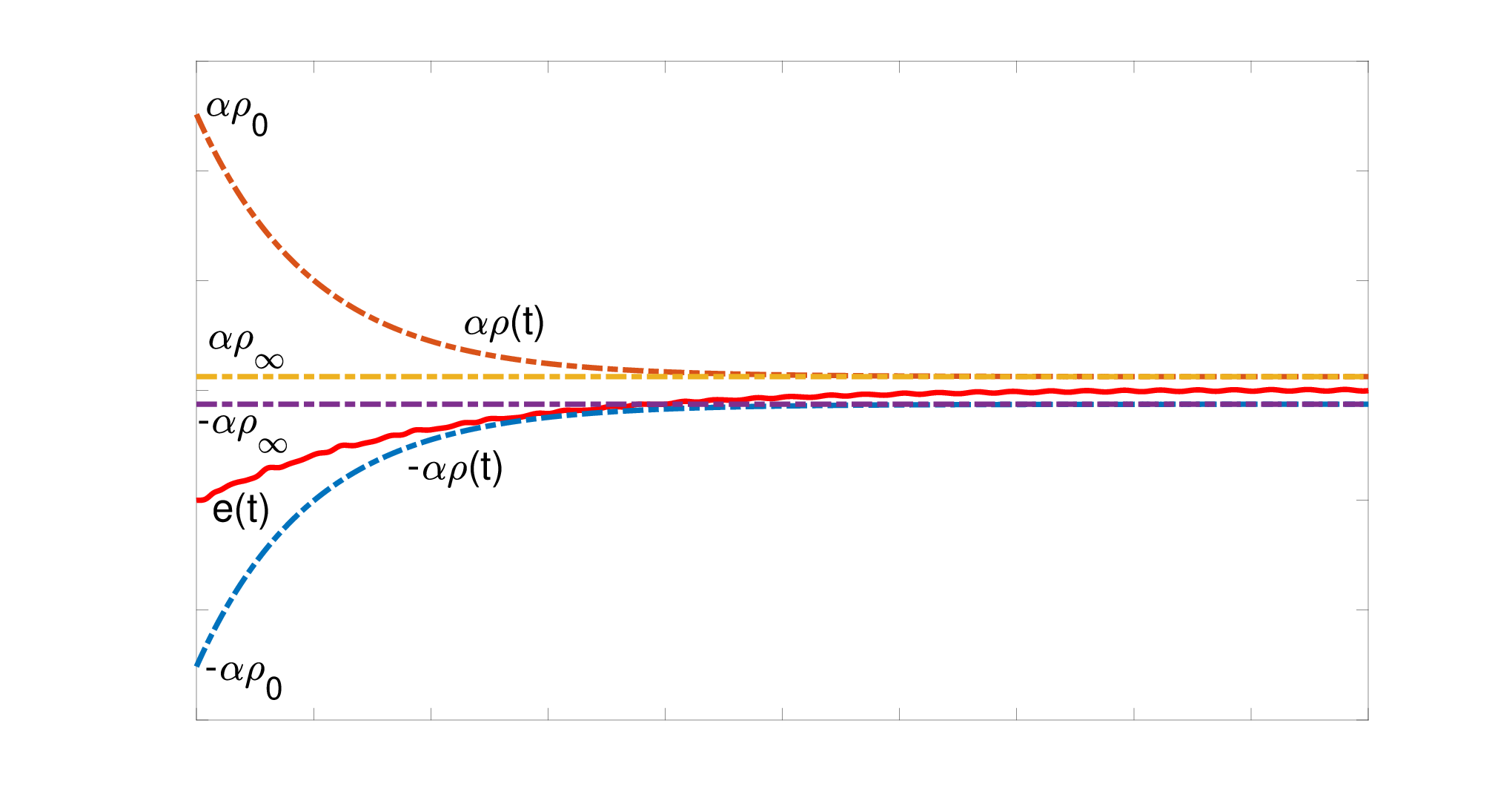
An intuitive explanation of (3) is displayed in Fig.1. Assuming that lies in the scope , the final maximum residual set is represented by , the maximum overshoot is confined to the scope , and the convergence speed of relates with the decreasing rate of that is determined by the value of . It should be clear that the parameter selection for (2) is determined by considering requirements of performance and safety together. For example, the determination of the scope for should also take the limited working space into consideration.
II-A Problem transformation
To facilitate the problem transformation, the following assumption about the desired trajectory is firstly given.
Assumption 2.
[10] The reference trajectory follows where is locally Lipschitz, and is bounded by .
For the considered OTCP, a concatenated state is introduced to transform it as an optimal regulation problem (ORP), which permits us to adopt RS-SP terms to tackle requirements of performances. The concatenated state is defined as
| (4) |
Calculating the time derivative of (4) yields
| (5) |
where , , and . The steady-state control policy with regard to the reference trajectory follows
| (6) |
Based on Assumption 1-2 and , we know that and is locally Lipschitz. Based on the boundness of , it is reasonable to conclude that .
In order to solve Problem 1, based on the auxiliary system (5) and risk sensitive terms, the PP-OTCP in Problem 1 is equivalent to the risk sensitive optimal regulation problem shown in Problem 2.
Problem 2 (risk sensitive optimal regulation problem (RS-ORP)).
In Problem 2, the PPs for the tracking errors are interpreted as constraints that are tackled by PPF based RS-SP terms under an optimization framework. The working scheme of is displayed in Fig.2. Intuitively speaking, acts as barriers at the constraint boundaries defined by PPFs, and confines the tracking error remain in the region that satisfies desired performances.

Remark 1.
The construction of is inspired by the barrier Lyapunov function (BLF) developed in [12]. is positive and approaches to infinity when the tracking error transgresses the boundaries of PPFs . The development of allows us to consider the PPs for full states easily. It should be clear that the reference trajectory is also included into (8), which permits us to adopt the optimal value function as a Lyapunov function candidate to provide the stability proof. The incorporation of into (8) results in an inevitable performance compromise problem, which can be dealt by setting the corresponding PPF as a loose one (a big ) with a sufficiently small .
II-B Hamilton Jacobi Bellman equation for auxiliary system
Considering Problem 2, for any admissible control policies defined as [13, Definition 1], the associated cost function is
| (9) |
Taking derivative of (9) with regard to yields the so-called nonlinear Lyapunov equation (LE),
| (10) |
where the operation operator denotes partial derivative with regard to , i.e. .
As for the RS-ORP in Problem 2, the associated optimal cost function is
| (11) |
Define the Hamiltonian as
| (12) |
An infinitesimal version of (11) is the so-called HJB equation and is written as the following form based on (12)
| (13) |
Assuming that the minimum of (11) exits and is unique. A closed form expression for the optimal control can be derived as
| (14) |
Inserting (14) into the LE equation (10), we can get the HJB equation as
| (15) |
III off policy adaptive critic learning
The HJB equation (15) is a nonlinear differential equation in terms of . This nonlinear nature makes it extremely difficult to solve directly. In this section, we follow the off policy adaptive critic learning technique developed in our prior work [11] to get the approximated solution by using the current data and experience data together. The usage of experience data to achieve weight convergence without incorporating external signals enable us to achieve PPs for full states and apply the control strategy into real applications.
III-A Value function approximation
According to the Weierstrass high-order approximation theorem [14], it is reasonable to conclude that there exists such that the value function can be approximated as
| (16) |
where is the approximation error. Activation functions of the artificial NN can be appropriately selected so that and its derivative
| (17) |
are both uniformly approximated. In the above, is the number of NN activation functions. As , both and uniformly. Without loss of generality, the following assumption is given in this paper.
Assumption 3.
The approximation error of NNs is assumed to be bounded by , and its derivative follows . It is assumed that activation functions and their gradients are also bounded, i.e. and .
III-B Off policy reinforcement learning
Since the ideal critic weight in (19) is unknown, let denote the estimated value of . The output of the critic learning agent is
| (20) |
The derivative of (20) based on the estimated weight is
| (21) |
Based on the estimated critic weight, (19) is rewritten as
| (22) |
Denoting , the approximation error is written as
| (23) |
Let be adapted to minimize the squared residual error . Then, the weight estimation update law is redesigned as
| (24) |
where is a constant positive definite gain matrix, are positive constant gains to trade off the relative importance between current data and experience data to the weight estimation update law. is the size of the experience buffers and , i.e. the maximum number of data points recorded into the experience buffers. The regression matrix and the approximation error denote the th collected data of the experience buffer and , respectively.
In order to analyse the weight convergence problem based on the weight estimation update law in (24), a rank condition is firstly clarified in Assumption 4.
Assumption 4.
Given an experience buffer , where is the th collected experience data of , there holds .
According to Theorem 2 provided in [11], the estimated weight of the critic learning agent is guaranteed to converge to its actual value based on the weight estimation update law (24). The control law can be derived directly based on the estimated critic weight as
| (25) |
Finally, we can get the control applied at the dynamics (1) as
| (26) |
The main conclusions of this paper are given as follows.
Theorem 1.
For the dynamics given by (5), the weight estimation update law is given by (24), and the approximated optimal control policy is in the form of (25). Assuming that Assumption 1-4 are satisfied, parameters are chosen as details in the proof. If the number of activation functions is sufficiently large, the following properties holds:
Proof.
Proof of (i). Considering the following Lyapunov function candidate
| (27) |
Taking time derivative of (27) along the system (5) yields
| (28) |
As for the first term
| (29) | ||||
For simplicity, denoting , it is assumed to be bounded as ; Let that is bounded as . Then, (29) is rewritten as
| (30) |
According to (18), the following equation establishes
| (31) | ||||
Finally, we can get
| (32) |
As for the second term , based on (24),
| (33) | ||||
where , which is bounded by .
Finally, substituting (32) and (33) into (28), based on the fact that , we can get
| (34) | ||||
where is positive, , and .
Since is positive definite, the above Lyapunov derivative is negative if
| (35) |
Thus, the critic weight estimation error converges to the residual set defined as
| (36) |
Denoting as the value of the Lyapunov function candidate at , it is a bounded function determined by initial values. According to the above derivation, establishes, which means that , always establishes, i.e. is a bounded function at any time. The boundness of implies that prescribed performance related constraints will not be violated. Otherwise, if any constraint violation happens. Thus, we can conclude that the prescribed performance of full states achieves.
Proof of (ii). The difference between the approximated optimal control and optimal control follows
| (37) | ||||
∎
IV Simulation results
A 2-DoF robot manipulator is chosen to show the effectiveness of the proposed control method. The Euler-Lagrange (E-L) model is given as
| (38) |
where , and are the vectors of joint angles, velocities, and accelerations respectively; is the inertia matrix with , , and ; is the matrix of centrifugal and Coriolis terms with , , , and ; stands for the dynamic friction; denotes the static friction. The explicit values for the robot dynamics are set as , , , , , , . The E-L equation (38) can be written in the form of (1) by setting , , and . For simulation, the reference trajectory is set as . Then, we get , .
IV-A OTCP case
In this section, the effectiveness of the proposed off policy adaptive critic learning architecture illustrated in Section III-B is tested to tackle the common OTCP. The robot manipulator (38) is driven to track the reference trajectory while minimizing the common quadratic cost function
| (39) |
where , . The basis set is chosen as
| (40) | ||||
The size of the experience buffer is set as . For the weight estimation update law (24), parameters are set as , , and . For simulation, the initial values are set as , . Simulation results for this typical OTCP is shown from Fig.3 to Fig.5.
The critic weight convergence result is shown in Fig.3. We know that after , the convergence of the estimated critic weight achieves without incorporating probing noises.

The trajectories of full states and their references are displayed in Fig.4, and the trajectory of the tracking error is shown in Fig.5. It is concluded that the proposed control strategy enable the robot manipulator track the reference trajectory precisely.


IV-B PP-OTCP case
In this part, the effectiveness of off policy RL based method to solve the PP-OTCP illustrated in Problem 1 is tested. For simulation, PPFs for full states are set as
| (41) |
To achieve optimal trajectory tracking control with PPs, the cost function is designed as
| (42) |
where , ; , ; , ; , ; .
For a fair comparison, the parameters are set as same with the OTCP case in Section IV-A. The parameter convergence result is shown in Fig.6. After 50 seconds, parameter convergence result achieves.
In order to show the effectiveness of the proposed method to achieve PPs, the comparison results are displayed from Fig.7 to Fig.10. As shown in Fig.7 and Fig.8, the trajectories of and based on the common quadratic cost function (39) violate the boundaries of PPFs, while our proposed method can effectively drive the robot manipulator to track reference trajectory and satisfy the performance requirements defined by PPFs.


V Conclusion
To achieve prescribed performances for full states of the optimal tracking control problem, an off policy risk sensitive RL based control strategy is developed in this paper. An auxiliary system is proposed to transform the optimal tracking control problem as an optimal regulation problem. The required prescribed performances are reflected by risk sensitive state penalty terms that are incorporated into the cost function of the transformed optimal regulation problem. The HJB equation is approximately solved based on an off policy adaptive critic learning architecture, which achieves weight convergence without incorporating external signals to satisfy the PE condition. Simulation results have proved the effectiveness of the proposed strategy. In the future, experiments will be conducted to show the effectiveness of the proposed strategy on a 3-DoF robot manipulator.
References
- [1] D. P. Bertsekas, D. P. Bertsekas, D. P. Bertsekas, and D. P. Bertsekas, Dynamic programming and optimal control. Athena scientific Belmont, MA, 1995, vol. 1, no. 2.
- [2] F. L. Lewis, D. Vrabie, and V. L. Syrmos, Optimal control. John Wiley & Sons, 2012.
- [3] C. P. Bechlioulis and G. A. Rovithakis, “Prescribed performance adaptive control for multi-input multi-output affine in the control nonlinear systems,” IEEE Transactions on Automatic Control, vol. 55, no. 5, pp. 1220–1226, 2010.
- [4] ——, “Robust adaptive control of feedback linearizable mimo nonlinear systems with prescribed performance,” IEEE Transactions on Automatic Control, vol. 53, no. 9, pp. 2090–2099, 2008.
- [5] Q. Guo, Y. Zhang, B. G. Celler, and S. W. Su, “Neural adaptive backstepping control of a robotic manipulator with prescribed performance constraint,” IEEE transactions on neural networks and learning systems, vol. 30, no. 12, pp. 3572–3583, 2018.
- [6] X. Huang, Y. Song, and J. Lai, “Neuro-adaptive control with given performance specifications for strict feedback systems under full-state constraints,” IEEE transactions on neural networks and learning systems, vol. 30, no. 1, pp. 25–34, 2018.
- [7] Y. Yang, Z. Liu, H. Xiong, and Y. Yin, “Adaptive singularity-free controller design of constrained nonlinear systems with prescribed performance,” Neurocomputing, 2020.
- [8] H. Dong, X. Zhao, and B. Luo, “Optimal tracking control for uncertain nonlinear systems with prescribed performance via critic-only adp,” IEEE Transactions on Systems, Man, and Cybernetics: Systems, 2020.
- [9] M. Wang and A. Yang, “Dynamic learning from adaptive neural control of robot manipulators with prescribed performance,” IEEE Transactions on Systems, Man, and Cybernetics: Systems, vol. 47, no. 8, pp. 2244–2255, 2017.
- [10] R. Kamalapurkar, H. Dinh, S. Bhasin, and W. E. Dixon, “Approximate optimal trajectory tracking for continuous-time nonlinear systems,” Automatica, vol. 51, pp. 40–48, 2015.
- [11] C. Li, F. Liu, Z. Zhou, and M. Buss, “Online single artificial neural network adaptive critic learning under additive disturbance, state constraints and input saturation,” arXiv preprint arXiv:2006.05681, 2020.
- [12] K. P. Tee, S. S. Ge, and E. H. Tay, “Barrier lyapunov functions for the control of output-constrained nonlinear systems,” Automatica, vol. 45, no. 4, pp. 918–927, 2009.
- [13] M. Abu-Khalaf and F. L. Lewis, “Nearly optimal control laws for nonlinear systems with saturating actuators using a neural network hjb approach,” Automatica, vol. 41, no. 5, pp. 779–791, 2005.
- [14] B. A. Finlayson, The method of weighted residuals and variational principles. SIAM, 2013, vol. 73.