On July 16, 2020 a friend with interest in science alerted me to an on-line ESA–NASA press conference that afternoon to announce first images from Solar Orbiter (SoLO): “closer than ever before”.

I had not expected this so soon after launch, but found a video movie of the ecliptic-projected orbit and saw that SolO dropped behind Earth so much at launch that it fell considerably from Earth orbit towards this relatively close pass (0.5 AU) then already.

A newspaper journalist then informed me embargoedly that the press release would boast “many little flames”.

Naturally I speculated about familiar solar little-flame phenomena: Ellerman bombs (EB, Rutten et al. 2013), quiet-Sun Ellerman-like brightenings (QSEB, Rouppe van der Voort et al. 2016), flaring active-region fibrils (FAF, Rutten 2016), IRIS bombs (IB, Peter et al. 2014), UV bursts (Young et al. 2018), tips of spicules-II in on-disk appearance as rapid blue excursion (RBE, Langangen et al. 2008) or rapid red excursion (RRE, Sekse et al. 2013b), and (ALMA) mm bursts (da Silva Santos et al. 2020).

Attending the press conference made clear that the little flames, coyly called “campfires”, sat in images from the EUI 174 Å HRI telescope implying million-K temperature and hence excluding EBs and QSEBs since these reconnection flames remain photospheric, not reaching EUV temperatures and even not breaking through the H$\alpha$ fibril canopy (which also hides them for ALMA, Rutten 2017b).

The tips of RBEs and RREs do reach out of the canopy and often reach EUV temperatures (Henriques et al. 2016), but these occur ubiquitously around network including quiet unipolar network, much less scarce than the dozen or so campfires in the approximately $0.5\times 0.5$ R_Sun SolO image that was shown.

The SolO campfires looked like FAFs to me.

I have inspected many FAFs in specific EBFAF detection movies multiplying SDO/AIA 1700 Å and 1600 Å after normalization, but the only detailed FAF descriptions are in Vissers et al. 2015. More in appendix A.

Here I report on my eventual finding these SolO campfires in SDO images. To cut the long story short: they are not FAFs. I speculate what instead.

The contents table serves as clickable outline; I therefore refrain from adding a descriptive contents outline here.

I keep the figures at the end to facilitate parallel text and figure inspection using a second pdf-reader instance (or printing the text if you prefer paper). For many images zoom-in to detail may be useful. Most are full-page to enable blinking by page flipping (how-to per viewer).

Immediately after the press conference I shared my FAF suspicion and asked whether the images would be public and whether I might have access to them for checking per SDO with my EBFAF detection technique. The quick answer from EUI PI David Berghmans was “yes” – but that it would take some months.

For a first look, being curious and impatient, I therefore saved the press-release high-resolution 174 Å image (figure 1), noting that the others shown were cutouts of it, asked for information where on the Sun and when it was taken, and downloaded the SDO/AIA 171 Å daily movie for the stipulated May 30, 2020 date to locate the SolO image scene.

The SolO EUI/HRI telescopes have 2048$\times$2048 0.5 arcsec pixels, the same angular pixel size as SDO/HMI (4096$\times$4096) and TRACE (1025$\times$1024) and close to the 0.6 arcsec of the four SDO/AIA telescopes to which SSW’s aia_prep.pro rescales HMI products. Hence, from about 0.5 AU the campfires should be twice sharper with SolO, but since they extend multiple pixels in the press-release image they should be visible in AIA 171 Å also.

The orbit movie suggested that SolO was about 40 degrees in advance of the Earth along the ecliptic, so I concentrated on pattern recognition of the SolO scene in figure 1 towards the West limb in the AIA 171 Å movie, hoping that the EUI/HRI telescope pointed near sub-SolO disk center and not towards the SolO West limb where the scene would already be backside for SDO.¹¹ 1 And for IRIS, Hinode, SST etc. if co-pointing had been requested – which I hoped since multi-telescope multi-diagnostic observation is the proper way to do solar physics in my view, motivating my efforts in SDO–other telescope co-alignment and before that in running EU networks.

I did not find the scene, also not for SolO’s full-disk 304 Å images in the press release.

I got no answer on my when and where question²² 2 Nor a reaction on this report although I shared a link while writing it. The admonition now under figure 1 came only post-posting. The current live link is this website post updating the arXiv post and also retaining an epilogue (pdf 14) on starting this report series. and I also realized that the SolO image might have been taken anywhere on the Sun with any orientation, perhaps even flipped or mirrored, and possibly beyond the SDO limb. Then Greg Slater (LMSAL) pointed out that the zoom movie shown in the press conference morphed between unrelated, disjoint scenes and so could not be used in location finding; the 304 Å full-disk view I had taken as guide might be from another date and have other orientation. He also suggested that the high-resolution image might have been taken during June at yet smaller SolO distance to the Sun but increasing SolO–Earth sight-line difference.

I therefore collected daily SD0 171 Å movies for many days and played them endlessly against the SolO image in many diverse orientations, trying visual pattern recognition – very confusing, the proverbial needle in a haystack. After many days of increasing frustration I gave up.

Eventually, on July 28 ESA mission scientist Daniel Müller informed me that the image was actually taken on May 30 as stipulated, around 14:54 UT. This enabled full-resolution full-cadence full-disk AIA sequence downloads and inspection at more detail than the SDO daily movies.

It took me a few days more but then I finally recognized the SolO scene in SDO 171 Å. After all my far-too-wide casting I found that the image was actually taken somewhat east of sub-SolO disk center, not flipped or mirrored, and had only small-angle rotation from solar North up as seen from the Earth and SDO.

Over the past decade I developed an extensive IDL pipeline to cross-align JSOC “im_patch” cutouts precisely between all SDO diagnostics and then co-align the results with small fields from other telescopes, in particular the Swedish 1-m Solar Telescope (SST). The first part is used here.

I aim to present this pipeline in another report in this series, but some detail is given already in my brief manual in the IDL directory where I make this software available.³³ 3 https://webspace.science.uu.nl/~rutte101/Recipes_IDL.html

In a nutshell, a single call of sdo_getdata.pro requests, collects, and cross-aligns SDO cutouts from JSOC, small ones at full cadence for the target area and large ones at lower cadence around disk center. The latter are used to find spatial offsets between the SDO diagnostics (“channels”) by cross-correlation of many small subfields, usually 30$\times$30 arcsec each, applying apparent height-of-formation differences and iterative removing outliers, as function of time during the requested sequence duration. Examples before and after are shown in figure 75. These “driftscenter” results are stored and used for the target cutouts, usually yielding cutout cross-alignment precision about 0.1 arcsec (an order better than the start-off co-registration by aia_prep.pro).

With sdo_getdata_rr,’2020.05.30_14:50’,15,375,148, xsize=700,ysize=700 I targeted a wider area around the SolO field during 15 minutes. The program took 42 min⁴⁴ 4 Deep Thought computation. to deliver the material used here.

In visual comparison I found that the best match with the SolO image in figure 1 occurred around time step 46 or 14:58:46 UT.

In addition I made full-disk images and charts at this best-match time with my sdo_diskfigs.pro which may be used for any non-eclipsed SDO moment and includes optional GONG H$\alpha$ download. It yielded the full-disk SDO overviews in figures 2–6 with the JSOC target cutout outlined.

There were two minor active regions near the East limb. The outlined SolO target shows nothing active beyond quiet network on the surface, but diffuse and also concentrated patches of EUV brightness – formerly “bright points” but “fires” now.

Normally, I obtain precise co-alignment with the “other” telescope (called STX for Solar Telescope X in my software and manual) which includes removal of small SDO wobbles left over from the JSOC whole-pixel cutout selection. Precise pixel-by-pixel SDO–STX comparisons are then possible and easily done with my versatile showex.pro⁵⁵ 5 The underlying engine is movex.pro, built on SSW’s ximovie.pro written by Øyvind Wikstøl and Viggo Hansteen for pre-Hinode Solar-B. sequence browser and blinker which can load very many different files and also cube parameters in memory together with jpg images or mpg movies and then zoom-in to pixel level.

In this case, however, I could not use my sdo_stx_align.pro because the SDO scene is foreshortened by its limbward viewing, differential across its large field, with respect to the SolO scene nearer disk center (probably with opposite foreshortening).

No pixel-by-pixel co-registration therefore, but it was easy to manually co-locate SolO campfires and larger ‘‘brushfires’’ ⁶⁶ 6 Ron Moore corrected my English by writing “brushfire” in a reaction. I had used “bushfire” for a fire larger than a “campfire” but smaller than “burning prairie” (obviously sardonic), but I did not appreciate that “bushfire” is Australian dialect for any wildfire including giant forest fires. Now I call the larger-than-campfire fires “brushfire”. precisely in SDO/AIA images with showex and then zoom-in to pixel detail to obtain pixel-clicked joint location output for matching ROI = “region of interest” cutouts of the SolO image and the SDO images.

These double coordinate pairs became the cutout centers for the 17 ROI cutout assemblies shown in figures 47–69. Their fields are sufficiently small to permit de-foreshortening and height-difference corrections detailed below.

Figure 1 shows the SolO press-release high-resolution image from the 174 Å EUI HRI telescope.⁷⁷ 7 The SolO/HRI pixels are 0.5 arcsec just as for SDO/HMI but twice smaller in km on the Sun at 0.5 AU distance. I could not add $(X,Y)$ axes to figure 1 because I do not know the sub-SolO XCEN and YCEN pointing values nor the precise pixel size and image orientation. The derotation applied here is a visual estimate. I see about a dozen campfires in subjective selection of tiny bright features. The 2048$\times$2048 px image measures about 402$\times$402 Mm² on the Sun, suggesting campfire density about $10^{-4}$ Mm^-2 or less than a thousand on the Sun if the remaining surface – in this quiet cycle phase – shows them likewise. Too scarce for a significant role in coronal heating.

Figures 7–15 show corresponding but somewhat larger SDO cutouts (plus a GONG H$\alpha$ cutout) at the best-match time in a selection that is diagnostically ordered bottom-to-top or cool-to-hot in naïve interpretation. For each SDO image the greyscaling is defined by the entire 15-min downloaded sequence to have common greyscales per diagnostic for the ROI cutouts in figures 48–65. The axes specify standard solar $(X,Y)$ coordinates with the origin at sub-Earth disk center, $Y$ pointing to the solar North pole, in arcsec⁸⁸ 8 Here called “SDO arcsec” for viewing from Earth..

IDL showex inspection with zoom-in and blinking is the best method for detailed comparison of these image sequences; the reader may do so by installing my pipeline, duplicate the above sdo_getdata command and inspect with showex. Flipping the below figure pages is a poor blinking emulation; zoom-in to detail is emulated as poorly in the ROI cutout assemblies in figures 48–65.

Unfortunately, the SolO image cannot be blinked at the pixel level to the SDO ones due to the considerable morphing by different and varying foreshortening. This also inhibits scatter correlations with Strous diagrams defined in Section 2 (pdf 2)⁹⁹ 9 Direct pdf page links as this one open the cited page on your screen with all pdf viewers I know – but not reliably under macOS. Mac users may instead be shunted to the first page and must then manually find the cited page. For the Mac-challenged I add the pdf page number in these links. Acrobat may require undoing security settings disabling the opening of web pages. of Rutten et al. 2019 and used here in figure 74.

Visual comparison with figure 1 shows that many campfires are also visible in the hotter AIA diagnostics, not only in AIA 171 Å (figure 14). In AIA 193 Å (figure 15) especially in dark areas where they stand out clearer.

Upshot: SolO was not required for noticing these small flames, although it does show them better. The gratifying good news is that the EUI HRI 174 Å telescope functions well.¹⁰¹⁰ 10 Just as the granulation and magnetic bright points in the press-released first DKIST images show nothing not already known from e.g., SST imaging, but do demonstrate promising telescope functioning. But also the same story – for lack of asked-for pointing information I did not find their scene in HMI images.

The SolO image appears clipped at the brightest levels. I therefore made the histograms in figure 16. The SolO histogram shows no sign of clipping but an extended highest-brightness tail not present in the AIA 171 Å histogram. I therefore added “cooler” and “hotter” AIA 131 and 193 Å histograms. The latter shows a similar tail, suggesting either nonlinear response in the SolO image or that its 174 Å bandpass includes hotter contributions than AIA’s 171 Å bandpass. The visibility of many SolO campfires in figure 15 suggests the latter.

Obviously the next question is whether the area imaged by SolO was somehow fortuitously special and lucky in uniquely harboring campfires not visible anywhere else or anytime before. The press release claimed “omnipresent miniature solar flares” but showed only the field of figure 1.

I therefore repeated sdo_getdata sequence collection and processing again for the best-match time but at sign-reversed $X$ and/or $Y$ to sample all four disk quadrants likewise, and also for the SolO pointing at the same date and time in the past three years. Figures 17–34 show the results. They are combined in “triples’ per location, arranged for easy blinking by page flipping (how-to viewer hints).

The first figure in each triple is the AIA 193 Å image, selecting this wavelength because it shows SolO campfires clearest of figures 7–15.

The second per triple shows my “SDO fire detector” construct to detect campfires and brushfires distinct from more ubiquitous chromospheric heating. It was inspired by EBFAF detection (appendix A) and figure 74 and proved useful in figure 69 of which the caption describes the construction. The greyscale clip and color threshold are defined for quiet network.

The detector construct appears to supply an amazingly good spatial separator between chromospheric heating and coronal heating in quiet-Sun regions. Chromospheric heating shows up as ubiquitous grey network patches, similarly present nearly everywhere. Coronal heating shows up as sparser small campfires and larger loop-bundle brushfires of which the cyan detector pixels emphasize the feet. More diffuse coronal heating with large-scale connectivity seen in 193 Å spreads around brushfires and may well be caused by these or preceding instances.

The third per triple shows the corresponding HMI magnetogram, clipped as described in the caption of figure 7.

Triple blinking is best done pairwise: 193 Å – detector and detector – magnetogram.

Blinking 193 Å – detector pairs in figures 17–34 shows that the detector does a good job in locating small campfires. Some of these fields contained active regions around which the thick haze of extended coronal loops in 193 Å hides small fires underneath, but the detector unveils some. Elsewhere the 193 Å and detector images in these six other-scene triples display similar tiny campfires at roughly similar (scarce) density as in figures 1 and 69.

Upshot: campfires seem indeed a sparse but omnipresent solar phenomenon. If SolO had been targeted elsewhere or launched earlier we would have had the same press conference.

Blinking detector – magnetogram pairs in figures 17–34 shows directly and unequivocally that all larger brushfires are located above or between mixed-polarity patches of multiple MCs (magnetic concentrations), suggesting EUV-visible heating due to bipolar MC happenings on the surface. All lie in extended grey patches in the detector images that represent dynamically heated chromosphere above and around network including “quiet” network (appendix B).

Only the smallest campfires seem to not always share bipolar magnetic feet (at HMI resolution and sensitivity), but these still lie preferentially in heated-chromosphere network patches.

Blinking 193 Å – detector pairs shows nearly 1:1 correspondence between campfire presence in 193 Å and cyan detector pixels, suggesting common heating to lower and higher temperatures.

The larger brushfires generally consist of close-packed short bright arches in 193 Å that connect opposite-polarity MC clusters in the magnetograms. In many the corresponding cyan detector pixels are grouped at the arch feet.

The campfires generally differ from the brushfires by not showing multiple-arch topography but just small single flames.

Another difference lies in their time behavior seen in showex viewing each downloaded time sequence: the campfire flames appear momentarily, mostly without repeat at the same location, whereas the brushfires live longer, usually throughout these 20-min sequence durations.

I also collected long-duration SDO sequences following the SolO scene six hours before and six hours after the SolO moment and found that most brushfire sites kept brushfiring continuously, irregularly but generally present during this time span.

The next question is whether campfires are a global quiet-Sun phenomenon still present during minima, or instead an activity phenomenon restricted to the activity belts and occurring with cycle modulation.

I therefore repeated sdo_getdata sequence collection and processing for similar-size North-pole and South-pole target areas during the maximum of cycle 24 and during the subsequent present minimum. Figures 35–46 show the results, again grouped together in 193 Å – detector – magnetogram triples for pairwise blinking.

These four polar areas also show campfires in quiet areas, including polar holes. Blinking 193 Å – detector pairs suggests that the smaller ones lie roughly as deep in the atmosphere in these diagnostics: they jump less limbward than the hazier 193 Å protrusions above them. I tried ${\tt heightdiff}=1000$ km for their construction (appendix A) but it made no difference in fire detection. Campfires are a chromospheric phenomenon¹¹¹¹ 11 Qua height, but not qua Lockyer 1868 since not seen in H$\alpha$..

The North-pole at maximum in figure 36 shows fewer fires towards the limb than the others – but there may be blocking along slanted lines-of sight to deep-lying fires, more at larger activity. Overall campfires seem a global phenomenon.

Blinking detector -- magnetogram polar pairs shows increasing limbward offsets, to the extent that near the limb fires and MC patterns are hard to match. Expected since the average height of the 304 Å chromosphere is multiple thousands of km, translating to projected shifts of multiple arcseconds there.¹²¹² 12 My pipeline presently uses limb value ${\tt heightdiff}=3600$ km for AIA 304 Å to HMI magnetogram cross-alignment, twice as much as in plane-parallel standard models but likely on the small side. An unpublished limb spectrum taken early in the IRIS mission by Bart De Pontieu and reduced by Han Uitenbroek shows Mg II h & k sticking out beyond 5000 km, whereas Mg II ionizes away at temperature 20 kK (coronal equilibrium) or lower (Saha-Boltzmann) about where He II comes up, so should appear “below” or near that unless non-E applies (appendix B). See also Alissandrakis 2019.

Thus, fires lie relatively deep for EUV phenomena, but not below the chromosphere as photospheric EBs and QSEBs do.

The ten-year full-disk high-cadence SDO database potentially permits an immensely rich harvest of campfires and brushfires, including appearance in other diagnostics as in these triples and also scene evolution before and after as in the ROI figures below. The fire detector offers an easy way to find SDO fires. The first projects suggested in section 9 are obvious strategies to elaborate on these few first-look trial samples shown here.

However, the 20 blink pairs of this section already furnish a vivid tell-tale overview of fire occurrence and properties. The tentative conclusion is that all or nearly all fires represent small-scale heating caused by bipolar MC interactions on the surface, likely occurring as globally as somewhat active mixed-polarity network does.

The larger, i.e., brushfires, clearly heat the corona locally above them and possibly elsewhere via long-loop connectivity. The smallest, i.e., campfires, are located at chromosphere heights and may possibly contribute coronal heating in minor fashion.

Chromosphere heating (of the ubiquitous grey network patches in the detector images, see appendix B) is instead wide-spread and not due to fires.

The next sections enlarge fires in the SolO field of figure 1 for more detailed inspection.

Figures 48–59 compare ROI = “region of interest” cutouts of SolO 174 Å campfires and corresponding co-located SDO diagnostics. These cutouts measure 24$\times$24 arcsec. Figure 47 shows their locations in the SolO 174 Å image.

The SDO cutout panels are de-foreshortened to mitigate slanted limbward viewing. This means that the original cutout pixels, which sample compressed solar surface in the limb direction with respect to transverse and at sub-SDO disk center, are increased in number in the limbward direction to stretch the surface they sample to the extent they would have in sub-SDO viewing from above.¹³¹³ 13 But not obtaining the actual view from above because the projection and blocking in slanted viewing remain. Remapping cannot repair that the Sun is 3D non-spherical although we zoom her 2D flat and describe her plane-parallel.

Since I do not know the sub-SolO $(X,Y)$ pointing I cannot apply deforeshortening to the SolO cutout at the top of these ROI figures. It is likely less but opposite.

The de-foreshortened SDO cutouts are ordered in time-delay columns, respectively 5, 2 and 1 min before the best-match time and then 1, 2, and 5 min later. These samplings emulate showex time-sliding while blinking.

From bottom to top the diagnostic order is as for figures 7–15, but adding the HMI continuum showing granulation at the bottom and replacing AIA 1600 Å with a construct called 16001700 and based on the 1600/1700 Å ratio to display excess AIA 1600 Å brightenings.

I switched to this construct instead of my usual EBFAF detection described in appendix A when I saw the scene in the AIA images. I would not have made my FAF suggestion if I had immediately been able to inspect SDO UV images for the correct date, time and disk location. When I finally could do so with figures 8–9 I saw no indication of any FAF whatsoever. Also no activity whatsoever in figure 7 – whereas the A in FAF stands for active region.

The new 16001700 construct therefore serves to note excess 1600 Å brightenings less obvious than FAFs. The brightness range in these ratio panels is set to $1.5-2.5$ based on inspection of EB- and FAF-rich data. The lower threshold excludes excess 1600/1700 brightening in ordinary magnetic concentrations (MC) masquerading as pseudo-EB (appendix A). The upper threshold does accommodate EBs and FAFs but such large enhancements are not reached here.

A complication in the construction of these ratio panels is that they need correction for the apparent limbward shifts of MC brightenings. This is also detailed in appendix A.

The yellow plus signs mark the locations that I clicked manually in zoom-in showex inspection of figure 1 and in parallel of figures 14–15, blinking the latter pair to find the best match, to select each ROI location.

The small yellow arrow to the upper right in the leftmost continuum panel at the bottom shows the local limb direction. Its length corresponds to the projection of a 3600 km tall upright structure (my heightdiff value for the 304 Å chromosphere). Roughly this arrow indicates the position shift one may expect between the surface and EUV samplings.

The axis scales are SDO-size arcsec for both, corresponding to 441.4 km on the Sun. For the SolO cutout they refer to the center of the full image. For the SDO cutouts the arcseconds are “stretched” by de-foreshortening but the cutout centers are non-stretched sub-SDO $(X,Y)$ values.

Per diagnostic the greyscale of each cutout is set by bytescaling the whole-field sequence, making brightenings comparable between different ROI figures.

My inspections of these assemblies were unusual for me because in all my SDO–STX (usually SST but also DST and IRIS) co-alignments I have always searched for bottom-up cause-effect order. My searches concerned happenings in the photosphere or chromosphere that would or did not cause hotter and higher EUV response.

The SolO campfires are dense and hot features of which the cause is the issue here – but the disturbance causing them may also come from above, as in the blobby coronal rain of Antolin et al. 2012 and flocculent flows of Vissers & Rouppe van der Voort 2012. The assembly rows are ordered top down from AIA 193 Å to the HMI continuum, but so comparisons should be made in both directions. At least the arrow of time from left to right should be unique.

Let me comment on these ROI figures one-by-one:

ROI-1. This is the arrow-marked campfire in the annotated version of the high-resolution image in the SolO press release.¹⁴¹⁴ 14 I think that (as usual) the selection was not a “typical” (= average) example but rather the nicest.

The SolO cutout on top shows an upward arc that is not present at the same time in AIA 171 Å while weakly present in AIA 193 Å and seen best in AIA 304 Å where it stays a few minutes.

The four AIA EUVs are all also bright at $\Delta t\!=\!\!-5$ min and then re-brighten during two minutes from $\Delta t\!=\!\!-1$ min, suggesting recurrence. Inspection with showex indeed showed larger previous brightening, maximal 7 min before the SolO moment.

There is a bipolar MC pair at the surface with significant excess brightening in AIA 1700 Å and also momentary 1600 Å excess brightening in the 16001700 construct that peaks at $\Delta t\!=\!\!-2$ min and then decays.

The granules in the bottom row are as uninteresting as always. I hoped to see vorticity around the campfire site but don’t see this. There may be granular convergence to the yellow cross but this is hard to tell at HMI image quality.

Top-down or bottom-up?

The MC pair at the exact location (account for the projection arrow in the first bottom panel), its brightening in 1700 Å and its larger-than-usual excess brightening in 1600 Å suggest bottom-up with the MCs as agent.

However, the 16001700 brightening is weaker than EBs which do not make it to hot AIA wavelengths, and if they did one would not expect the precise co-spatiality of the bright grain in 171 Å and 193 Å seen here. FAFs do show effects in these high-temperature diagnostics but as distant expanding arcs (Vissers et al. 2015). Apparent co-spatiality is also seen in the 193 Å – detector blink pairs in the limb triples (figures 35–46).

Top-down supposedly means for such a small disturbance propagating down that it follows field lines and so naturally ends up in a surface MC since all field lines are rooted in such. The earlier 1600 and 1700 brightenings may then follow from a similar earlier disturbance dropping from above. Indeed, in showex they show the 7-min earlier brightening too, reaching maximum at small (about 12 s) delay.¹⁵¹⁵ 15 Showex can also plot timelines per pixel. The AIA UV exposures sampled at 24 s cadence are interpolated with all others to the 12-s 171 Å timings in my pipeline. All samplings along columns are synchronous, as are the triples in figures 17–46.

The AIA 304 Å row inspired me to add appendix B. The campfire feature is most extended and complex here, and there are larger fuzzy patches around it. In both bottom-up and top-down scenarios one would expect it to show up between the UVs and the hotter EUVs in size and appearance. The simultaneous visibility of the arc in the SolO image and in 304 Å might then suggest that SolO includes a cooler line in its 174 Å passband.

However, to me the fuzzy long-lived AIA 304 Å appearance suggests response to irradiation from above followed by non-E visibility extension as described in appendix B.

ROI-2. Not a single flame but a more complex multi-feature campfire in the SolO cutout at the top. AIA 193 Å mimics it best. Its continuous presence and the presence of mixed-polarity MCs on the surface suggest that this is a bottom-up feature of the type I call brushfire and show in the next section. The agent causing it happened before these sequences.

ROI-3. Weak brightening at the center of a fuzzy diabolo-shaped feature. Both are clearest in the SolO cutout. Nothing in the 16001700 panel, weak monopolar MCs on the surface. The diffuse surrounding 304 Å brightness again suggests hot irradiation from above.

ROI-4. Rather like a weak version of ROI-1 but without precursor. A nearby MC on the surface surrounded by weak opposite-polarity MCs. Again the feature is most extended and fuzzy in 304 Å.

ROI-5. Similar to ROI-4. Brightest in AIA 131 Å at just the SolO moment.

ROI-6. Similar again but embedded in a longer rather persistent feature .

ROI-7. Local brightening in the SolO cutout but not standing out in any SDO panel. Perhaps foreshortening blocking by the fuzzy surroundings best seen in the 304 Å panel.

ROI-8. Present in the SDO EUV panels, also earlier, then fading. Again 304 Å shows the most extended surroundings. The 16001700 panel has an excess feature but dislocated.

ROI-9. Already present at the start, with some mixed-polarity field on the surface. Perhaps a small brushfire.

ROI-10. Weak but also persistent from the start, with some mixed-polarity MCs on the surface.

ROI-11. Truly a SolO campfire because there is nothing in any AIA diagnostic including the fire detector in figure 69. AIA 171 Å shows weak streaking in the same direction, that’s all. Nothing at its location in the HMI magnetogram. The bright SolO streak may be just that, higher up and may be blocked by foreground opacity in the slanted AIA viewing through the gas above the large brushfire of ROI-D.

ROI-12. Local brightening in a small brushfire.

In this section I add similar cutout figures for some of the larger bright patches in figure 1. I call these “brushfire” after language correction by Ron Moore (footnote 6). They likely all are regular “coronal bright points” but I keep to my phenomenological name in this purely observational inventory.

I selected five called ROI-A – ROI-E. Their locations and the corresponding ROI cutouts in the SolO 174 Å image are shown in Figure 60. These cutouts measure 36$\times$36 arcsec².

Figures 61–65 again show a selection of SDO diagnostics. The column timings are now respectively 9, 6, and 3 min before the best-match time in the last column.

All five EUV-bright patches remain more or less the same during these nine minutes, so that discussing their origin is literally beyond this study: for each it took place or started before my downloaded SDO sequences.

However, all five sit above locations with somewhat enhanced mixed-polarity network. Figures 66–69 show the HMI magnetogram of figure 7 and various EUV diagnostics with all ROI boxes superimposed. Blinking shows that also all other bright EUV patches of brushfire size sit above similar mixed-polarity network concentrations, whereas campfires, as SolO prototype number 1, can be at quieter monopolar locations.

It therefore seems likely that the brushfires are all bottom-up cases resulting from magnetodynamic opposite-polarity interactions on the surface. The same is suggested by the high degree of correspondence between larger fires and somewhat denser mixed-polarity MC assemblies in the “other” SDO scenes in figures 17–46.

Most coronal fires in this report seem controlled bottom-up by MC interactions of quiet mixed-polarity network on the surface, as suggested for X-ray/coronal bright points since Skylab (e.g., Krieger et al. 1971). They seem to furnish most quiet-Sun coronal heating.

Coronal fire heating is very distinct from ubiquitous chromospheric heating around all network in the fire detector images that separate these classes remarkably well by fire feet marking.

Whether coronal fires mark MC reconnection that may be diagnosed from cancelation, fly-by reconnection that may be diagnosed from MC trajectories, reconnective twisting that may be diagnosed from swirling, reconnective or ion-neutral slingshotting that may be diagnosed from simulation, or Alvénic wave heating that may be diagnosed from propagation is beyond this study.²⁰²⁰ 20 Or all contribute adhering to the “Principle of Solar Communicativity” (pdf 9) formulated at the only solar IAU symposium ever in the USSR (Rutten 1990).

Campfires represent the smallest, scarcest, briefest, least important specimens of the coronal bright point phenomenon. The one-pixel EIT Fe XII 195 Å coronal bright points of Falconer et al. 1998 were a decades-earlier campfire detection. SDO shows them daily in multitudes for a decade already. Blinking the triples in figures 17–46 suggests that they reside at chromospheric heights and do not contribute noticeable coronal heating.

Some smallest campfires, including some original SolO campfires, may represent exceptions to bipolar footpoint interaction and perhaps mark larger-scale surface vortices or impacting field-guided CME return blobs.

I suggest that coronal brushfire heating corresponds to sets 1 and 2 in Fig. 12 (pdf 13) of Frogner et al. 2020 with particle-beam foot heating giving the fire pinpoint functionality of the chromospheric 304$\times$131 detector product.

For the campfires I suggest that most represent small localized chromosphere heating as in set 3 of this figure. It comes electrically from above, is quickly radiated away, and does not affect the H$\alpha$ chromosphere – making “St. Elmo’s fires” a better nickname for these harmless little electric flames. They may be diagnosed by charting IRIS Si IV Dopplershifts at AIA campfires (Testa et al. 2014, Polito et al. 2018).

The obvious recommendation from this study is to not await properly validated SolO images or future SolO campfire observations but to study them in the SDO database using fire detection as in figure 69 to find them.

If my institute would offer access to studentships and students²¹²¹ 21 If a student of this report desires to use material or techniques used here I likely will cooperate. I would propose as projects:

1. 1.

   obtain longer SDO sequences than here and use ROI cutout timeline analysis to study fire recurrence and doubling where multiple feet heating occurs;

2. 2.

   apply the SDO fire detector of figure 69 to the entire SDO database to assemble campfire statistics as function of the cycle, latitude, open/closed field geometry, etcetera;

3. 3.

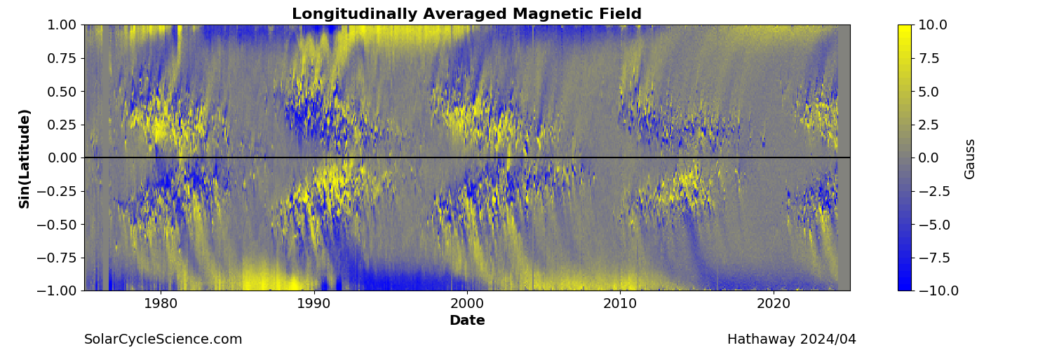
   do the same for more interesting brushfires in relation to larger-scale coronal connectivity patterns. Also produce latitude–time fire activity diagrams in the style of David Hathaway’s beautiful magnetic butterfly diagram;

4. 4.

   try to find campfires that follow on CMEs with subsequent flocculent rain, first for trial demonstration and when successful with machine learning for the entire SDO database;

5. 5.

   search for granular and/or MC vortices at fire sites. For SolO use simultaneous SolO/PHI granulation imaging. For SDO use simultaneous Hinode/SOT or groundbased granulation imaging. Expand to chromospheric vortices where chromospheric diagnostics are available. Expand if possible to the SDO database when successful;

6. 6.

   use Bifrost or MURaM simulations to replicate and demonstrate the apparent brightening differences and limb shifts of MCs between different ultraviolet wavelengths, including the AIA, TRACE and IRIS/SLI ones;

7. 7.

   use SST/CHROMIS observations in the extended Ca II H & K wings to study MC stratifications following Sheminova et al. 2005, extend these to larger height with IRIS Mg II h & k scans, do so for quiet network and brushfire-feet mixed-polarity network, also cover center-to-limb sampling, and compare with Bifrost or MURaM mixed-network simulations with H & K and h & k wing synthesis using RH 1.5D (Pereira & Uitenbroek 2015);

8. 8.

   develop a FAFDETECT algorithm and search the SDO database for slow wind sources as in Brooks et al. 2015;

9. 9.

   use machine learning to search the SDO database for retarded correlation of AIA 304 Å brightenings after AIA 1600 Å brightenings, and also of AIA 304 Å brightenings after flocculent CME return flows in the hotter AIA’s. Best done with early SDO data when AIA 304 Å had higher signal-to-noise;

10. 10.

    use automation on the SDO and GONG H$\alpha$ databases to select the best H$\alpha$ images, de-stretch and co-align these precisely with AIA 304 Å  and quantify pattern equality including relative time delay. Better would be to find sharper joint data sets for these two lines and use those. Yet better would be to add ALMA imaging.

References

- Alissandrakis (2019) Alissandrakis, C. E. 2019, SoPh, 294, 161 ADS
- Antolin et al. (2012) Antolin, P., Vissers, G., & Rouppe van der Voort, L. 2012, SoPh, 280, 457 ADS
- Attie et al. (2009) Attie, R., Innes, D. E., & Potts, H. E. 2009, A&A, 493, L13 ADS
- Avrett (1965) Avrett, E. H. 1965, SAO Special Report, 174, 101 ADS
- Avrett & Loeser (2008) Avrett, E. H. & Loeser, R. 2008, ApJS, 175, 229 ADS
- Bakke et al. (2018) Bakke, H., Frogner, L., & Gudiksen, B. V. 2018, A&A, 620, L5 ADS
- Bello González et al. (2013) Bello González, N., Danilovic, S., & Kneer, F. 2013, A&A, 557, A102 ADS
- Berger et al. (2004) Berger, T. E., Rouppe van der Voort, L. H. M., Löfdahl, M. G., et al. 2004, A&A, 428, 613
- Bonet et al. (2010) Bonet, J. A., Márquez, I., Sánchez Almeida, J., et al. 2010, ApJL, 723, L139 ADS
- Bose et al. (2019) Bose, S., Henriques, V. M. J., Joshi, J., & Rouppe van der Voort, L. 2019, A&A, 631, L5
- Brandt et al. (1994) Brandt, P. N., Rutten, R. J., Shine, R. A., & Trujillo Bueno, J. 1994, in NATO Advanced Science Institutes (ASI) Series C, Vol. 433, Solar and stellar magnetism, ed. R. J. Rutten & C. J. Schrijver, 251
- Brandt et al. (1988) Brandt, P. N., Scharmer, G. B., Ferguson, S., et al. 1988, Nat, 335, 238 ADS
- Brooks et al. (2015) Brooks, D. H., Ugarte-Urra, I., & Warren, H. P. 2015, Nature Communications, 6, 5947 ADS
- Bünte et al. (1993) Bünte, M., Solanki, S. K., & Steiner, O. 1993, A&A, 268, 736
- Carlsson & Stein (1994) Carlsson, M. & Stein, R. F. 1994, in Chromospheric Dynamics, ed. M. Carlsson, Proc. Miniworkshop (Oslo: Inst. Theor. Astrophys.), 47–77 ADS
- Carlsson & Stein (1995) Carlsson, M. & Stein, R. F. 1995, ApJL, 440, L29 ADS
- Carlsson & Stein (1997) Carlsson, M. & Stein, R. F. 1997, ApJ, 481, 500 ADS
- Carlsson & Stein (2002) Carlsson, M. & Stein, R. F. 2002, ApJ, 572, 626 ADS
- Carlsson et al. (2004) Carlsson, M., Stein, R. F., Nordlund, Å., & Scharmer, G. B. 2004, ApJL, 610, L137 ADS
- Chintzoglou et al. (2020) Chintzoglou, G., De Pontieu, B., Martínez-Sykora, J., et al. 2020, arXiv e-prints, arXiv:2005.12717 ADS
- da Silva Santos et al. (2020) da Silva Santos, J. M., de la Cruz Rodríguez, J., White, S. M., et al. 2020, A&A, 643, A41 ADS
- Danilovic (2017) Danilovic, S. 2017, A&A, 601, A122 ADS
- De Pontieu et al. (2012) De Pontieu, B., Carlsson, M., Rouppe van der Voort, L. H. M., et al. 2012, ApJL, 752, L12 1 ADS
- Ellerman (1917) Ellerman, F. 1917, ApJ, 46, 298 ADS
- Falconer et al. (1998) Falconer, D. A., Moore, R. L., Porter, J. G., & Hathaway, D. H. 1998, ApJ, 501, 386 ADS
- Fontenla et al. (1993) Fontenla, J. M., Avrett, E. H., & Loeser, R. 1993, ApJ, 406, 319 ADS
- Frogner et al. (2020) Frogner, L., Gudiksen, B. V., & Bakke, H. 2020, A&A, 643, A27 ADS
- Hansteen et al. (2017) Hansteen, V. H., Archontis, V., Pereira, T. M. D., et al. 2017, ApJ, 839, 22 ADS
- Henriques et al. (2016) Henriques, V. M. J., Kuridze, D., Mathioudakis, M., & Keenan, F. P. 2016, ApJ, 820, 124 ADS
- Hill et al. (2019) Hill, F., Hammel, H., Martínez-Pillet, V., et al. 2019, in Bulletin of the American Astronomical Society, Vol. 51, 74
- Holweger (1967) Holweger, H. 1967, Z. Astrophys., 65, 365 ADS
- Holweger & Müller (1974) Holweger, H. & Müller, E. A. 1974, SoPh, 39, 19 ADS
- Hong et al. (2014) Hong, J., Ding, M. D., Li, Y., Fang, C., & Cao, W. 2014, ApJ, 792, 13 ADS
- Joshi et al. (2020) Joshi, J., Rouppe van der Voort, L. H. M., & de la Cruz Rodríguez, J. 2020, A&A, 641, L5 ADS
- Keller et al. (2004) Keller, C. U., Schüssler, M., Vögler, A., & Zakharov, V. 2004, ApJL, 607, L59 ADS
- Kim et al. (2015) Kim, Y.-H., Yurchyshyn, V., Bong, S.-C., et al. 2015, ApJ, 810, 38 ADS
- Kostik & Orlova (1975) Kostik, R. I. & Orlova, T. V. 1975, SoPh, 45, 119 ADS
- Krieger et al. (1971) Krieger, A. S., Vaiana, G. S., & van Speybroeck, L. P. 1971, in Solar Magnetic Fields, ed. R. Howard, Vol. 43, 397 ADS
- Langangen et al. (2008) Langangen, Ø., De Pontieu, B., Carlsson, M., et al. 2008, ApJL, 679, L167 ADS
- Leenaarts et al. (2007) Leenaarts, J., Carlsson, M., Hansteen, V., & Rutten, R. J. 2007, A&A, 473, 625 ADS
- Leenaarts et al. (2012) Leenaarts, J., Carlsson, M., & Rouppe van der Voort, L. 2012, ApJ, 749, 136 ADS
- Leenaarts et al. (2015) Leenaarts, J., Carlsson, M., & Rouppe van der Voort, L. 2015, ApJ, 802, 136 ADS
- Leenaarts et al. (2006a) Leenaarts, J., Rutten, R. J., Carlsson, M., & Uitenbroek, H. 2006a, A&A, 452, L15
- Leenaarts et al. (2006b) Leenaarts, J., Rutten, R. J., Sütterlin, P., Carlsson, M., & Uitenbroek, H. 2006b, A&A, 449, 1209
- Lites et al. (2008) Lites, B. W., Kubo, M., Socas-Navarro, H., et al. 2008, ApJ, 672, 1237
- Lites et al. (1999) Lites, B. W., Rutten, R. J., & Berger, T. E. 1999, ApJ, 517, 1013
- Liu et al. (2019a) Liu, J., Carlsson, M., Nelson, C. J., & Erdélyi, R. 2019a, A&A, 632, A97 ADS
- Liu et al. (2019b) Liu, J., Nelson, C. J., Snow, B., Wang, Y., & Erdélyi, R. 2019b, Nature Communications, 10, 3504 ADS
- Livingston & Wallace (1987) Livingston, W. & Wallace, L. 1987, ApJ, 314, 808
- Lockyer (1868) Lockyer, J. N. 1868, Proceedings of the Royal Society of London Series I, 17, 131 ADS
- Loukitcheva et al. (2015) Loukitcheva, M., Solanki, S. K., Carlsson, M., & White, S. M. 2015, A&A, 575, A15 ADS
- Low (1985) Low, B. C. 1985, ApJ, 293, 31
- Madjarska (2019) Madjarska, M. S. 2019, Living Reviews in Solar Physics, 16, 2 ADS
- Martínez-Sykora et al. (2020a) Martínez-Sykora, J., De Pontieu, B., de la Cruz Rodriguéz, J., & Chintzoglou, G. 2020a, ApJL, 891, L8 ADS
- Martínez-Sykora et al. (2020b) Martínez-Sykora, J., Leenaarts, J., De Pontieu, B., et al. 2020b, ApJ, 889, 95 ADS
- McMath et al. (1960) McMath, R. R., Mohler, O. C., & Dodson, H. W. 1960, Proceedings of the National Academy of Science, 46, 165 ADS
- Molnar et al. (2019) Molnar, M. E., Reardon, K. P., Chai, Y., et al. 2019, ApJ, 881, 99 ADS
- Muller (1984) Muller, R. 1984, in Active Phenomena in the Outer Atmosphere of the Sun and Stars, 382
- Nelson et al. (2013a) Nelson, C. J., Doyle, J. G., Erdélyi, R., et al. 2013a, SoPh, 283, 307 ADS
- Nelson et al. (2015) Nelson, C. J., Scullion, E. M., Doyle, J. G., Freij, N., & Erdélyi, R. 2015, ApJ, 798, 19 ADS
- Nelson et al. (2013b) Nelson, C. J., Shelyag, S., Mathioudakis, M., et al. 2013b, ApJ, 779, 125 ADS
- November (2004) November, L. J. 2004, A&A, 417, 333
- Panasenco et al. (2014) Panasenco, O., Martin, S. F., & Velli, M. 2014, SoPh, 289, 603 ADS
- Pariat et al. (2009) Pariat, E., Masson, S., & Aulanier, G. 2009, ApJ, 701, 1911 ADS
- Pereira & Uitenbroek (2015) Pereira, T. M. D. & Uitenbroek, H. 2015, A&A, 574, A3 ADS
- Peter et al. (2014) Peter, H., Tian, H., Curdt, W., et al. 2014, Science, 346, 1255726 ADS
- Polito et al. (2018) Polito, V., Testa, P., Allred, J., et al. 2018, ApJ, 856, 178 ADS
- Rezaei & Beck (2015) Rezaei, R. & Beck, C. 2015, A&A, 582, A104 ADS
- Rouppe van der Voort et al. (2020) Rouppe van der Voort, L. H. M., De Pontieu, B., Carlsson, M., et al. 2020, A&A, 641, A146 ADS
- Rouppe van der Voort et al. (2016) Rouppe van der Voort, L. H. M., Rutten, R. J., & Vissers, G. J. M. 2016, A&A, 592, A100 ADS
- Rutten (1990) Rutten, R. J. 1990, in IAU Symposium, Vol. 138, Solar Photosphere: Structure, Convection, and Magnetic Fields, ed. J. O. Stenflo, 501–516 ADS
- Rutten (1995) Rutten, R. J. 1995, in ESA Special Pub., Vol. 376, Helioseismology, ed. J. T. Hoeksema, V. Domingo, B. Fleck, & B. Battrick, 151–163
- Rutten (1999) Rutten, R. J. 1999, in Astron. Soc. Pacific Conf. Series, Vol. 184, Magnetic Fields and Oscillations, ed. B. Schmieder, A. Hofmann, & J. Staude, Third Adv. in Solar Physics Euroconf., 181–200 ADS
- Rutten (2003) Rutten, R. J. 2003, Radiative Transfer in Stellar Atmospheres (Utrecht: Lecture notes Utrecht University) ADS
- Rutten (2013) Rutten, R. J. 2013, in Astron. Soc. Pacific Conf. Series, Vol. 470, 370 Years of Astronomy in Utrecht, ed. G. Pugliese, A. de Koter, & M. Wijburg, 49–58 ADS
- Rutten (2016) Rutten, R. J. 2016, A&A, 590, A124 ADS
- Rutten (2017a) Rutten, R. J. 2017a, in IAU Symposium, Vol. 327, Fine structure and dynamics of the solar atmosphere, ed. S. Vargas Domínguez, A. G. Kosovichev, P. Antolin, & L. Harra, 1–15 ADS
- Rutten (2017b) Rutten, R. J. 2017b, A&A, 598, A89 ADS
- Rutten (2019) Rutten, R. J. 2019, SoPh, 294, 165 1 ADS
- Rutten et al. (2011) Rutten, R. J., Leenaarts, J., Rouppe van der Voort, L. H. M., et al. 2011, A&A, 531, A17
- Rutten & Rouppe van der Voort (2017) Rutten, R. J. & Rouppe van der Voort, L. H. M. 2017, A&A, 597, A138 ADS
- Rutten et al. (2019) Rutten, R. J., Rouppe van der Voort, L. H. M., & De Pontieu, B. 2019, A&A, 632, A96 ADS
- Rutten et al. (2015) Rutten, R. J., Rouppe van der Voort, L. H. M., & Vissers, G. J. M. 2015, ApJ, 808, 133 1 ADS
- Rutten & Uitenbroek (1991) Rutten, R. J. & Uitenbroek, H. 1991, SoPh, 134, 15 ADS
- Rutten & Uitenbroek (2012) Rutten, R. J. & Uitenbroek, H. 2012, A&A, 540, A86 ADS
- Rutten et al. (2013) Rutten, R. J., Vissers, G. J. M., Rouppe van der Voort, L. H. M., Sütterlin, P., & Vitas, N. 2013, in J. Physics Conf. Series, Vol. 440, Eclipse on the Coral Sea: Cycle 24 Ascending, ed. P. S. Cally, R. Erdélyi, & A. A. Norton, 1–13 ADS
- Schrijver et al. (1997) Schrijver, C. J., Title, A. M., van Ballegooijen, A. A., Hagenaar, H. J., & Shine, R. A. 1997, ApJ, 487, 424 ADS
- Sekse et al. (2013a) Sekse, D. H., Rouppe van der Voort, L., & De Pontieu, B. 2013a, ApJ, 764, 164 ADS
- Sekse et al. (2013b) Sekse, D. H., Rouppe van der Voort, L., De Pontieu, B., & Scullion, E. 2013b, ApJ, 769, 44 ADS
- Sheminova et al. (2005) Sheminova, V. A., Rutten, R. J., & Rouppe van der Voort, L. H. M. 2005, A&A, 437, 1069 ADS
- Shimizu et al. (2002) Shimizu, T., Shine, R. A., Title, A. M., Tarbell, T. D., & Frank, Z. 2002, ApJ, 574, 1074 ADS
- Solanki (1993) Solanki, S. K. 1993, Space Sci. Rev., 63, 1
- Spruit (1976) Spruit, H. C. 1976, SoPh, 50, 269
- Spruit (1977) Spruit, H. C. 1977, PhD thesis, - ADS
- Steiner (2005) Steiner, O. 2005, A&A, 430, 691 ADS
- Stellmacher & Wiehr (1991) Stellmacher, G. & Wiehr, E. 1991, A&A, 251, 675
- Stenflo (1984) Stenflo, J. O. 1984, Advances in Space Research, 4, 5
- Stenflo et al. (1984) Stenflo, J. O., Solanki, S., Harvey, J. W., & Brault, J. W. 1984, A&A, 131, 333
- Testa et al. (2014) Testa, P., De Pontieu, B., Allred, J., et al. 2014, Science, 346, 1255724 ADS
- Title & Berger (1996) Title, A. M. & Berger, T. E. 1996, ApJ, 463, 797
- Tziotziou et al. (2018) Tziotziou, K., Tsiropoula, G., Kontogiannis, I., Scullion, E., & Doyle, J. G. 2018, A&A, 618, A51 ADS
- Unruh et al. (1999) Unruh, Y. C., Solanki, S. K., & Fligge, M. 1999, A&A, 345, 635 ADS
- Vargas Domínguez et al. (2011) Vargas Domínguez, S., Palacios, J., Balmaceda, L., Cabello, I., & Domingo, V. 2011, MNRAS, 416, 148 ADS
- Vernazza et al. (1981) Vernazza, J. E., Avrett, E. H., & Loeser, R. 1981, ApJS, 45, 635 ADS
- Vissers & Rouppe van der Voort (2012) Vissers, G. & Rouppe van der Voort, L. 2012, ApJ, 750, 22 ADS
- Vissers et al. (2013) Vissers, G. J. M., Rouppe van der Voort, L. H. M., & Rutten, R. J. 2013, ApJ, 774, 32 1 ADS
- Vissers et al. (2019) Vissers, G. J. M., Rouppe van der Voort, L. H. M., & Rutten, R. J. 2019, A&A, 626, A4 ADS
- Vissers et al. (2015) Vissers, G. J. M., Rouppe van der Voort, L. H. M., Rutten, R. J., Carlsson, M., & De Pontieu, B. 2015, ApJ, 812, 11 1 ADS
- Vitas et al. (2009) Vitas, N., Viticchiè, B., Rutten, R. J., & Vögler, A. 2009, A&A, 499, 301 ADS
- Watanabe et al. (2011) Watanabe, H., Vissers, G., Kitai, R., Rouppe van der Voort, L., & Rutten, R. J. 2011, ApJ, 736, 71 ADS
- Wedemeyer et al. (2013) Wedemeyer, S., Scullion, E., Rouppe van der Voort, L., Bosnjak, A., & Antolin, P. 2013, ApJ, 774, 123 ADS
- Wedemeyer-Böhm et al. (2012) Wedemeyer-Böhm, S., Scullion, E., Steiner, O., et al. 2012, Nat, 486, 505 ADS
- Yang et al. (2013) Yang, H., Chae, J., Lim, E.-K., et al. 2013, SoPh, 288, 39 ADS
- Young et al. (2018) Young, P. R., Tian, H., Peter, H., et al. 2018, Space Sci. Rev., 214, 120 1 ADS
- Zwaan (1965) Zwaan, C. 1965, Sunspot models; a study of sunspot spectra
- Zwaan (1967) Zwaan, C. 1967, SoPh, 1, 478
- Zwaan (1978) Zwaan, C. 1978, SoPh, 60, 213
Figure blinking by page flipping
Viewer-dependent; try single-page, fit-to-page, full-page, full-screen, presentation mode, thumbnail panel, left-right, up-down, page up-down.
- •
Gnome evince: zoom-in (CTRL +), page-blink with up-down in the thumbnail side panel or full-page and left-right;
Acrobat acroread: full-page (CTRL L), zoom-in (CTRL +), blink left-right;
Ubuntu qpdfview: full-screen, zoom-in (CTRL right), blink left-right;
Chrome and Firefox pdf viewers: left-right, or full-page and up-down or page up-down;
MacOS: Firefox left-right or full-page and up-down, Safari full-page up-down, Preview full-page up-down or mouse scroller, zoom-in and left-right.
Caveat disclaimer: EUI PI David Berghmans reprimanded me later that this image “is not properly validated” and showing it here is “unfair to the intrinsic quality of the EUI instrument” – but it serves here only to display the “campfires” shown and advertised during the SolO press conference, and as proof that I eventually did find this non-specified SolO scene in SDO (compare with figure 15). Proper validation may make this image yet better and enable proper axes, but will not affect any other image here nor SDO campfires in these (which by existing guarantee that the SolO ones can’t validate away).
Copyright: Solar Orbiter/EUI Team/ESA & NASA; CSL, IAS, MPS, PMOD/WRC, ROB, UCL/MSSL.
This stringent pixel-value selection appears useful as EUV fire detector. Spatial extent and temporal duration may then discriminate between small momentary campfires versus wider and more persistent brushfires.
The grey patches everywhere else represent dynamic chromosphere around quiet network. They are ubiquitously present with similar appearance in spreading around network MC concentrations, defining grey in this image well-suited as heated-chromosphere locator. It is hot since it is seen here and also as grey background in 171 Å (figure 14), AIA 221 Å and AIA 335 Å, but it is also darkly visible in H (blink with figure 11). This dual visibility is discussed in appendix B.
The darkest patches between the grey ones generally match dark features present in most other AIA EUVs and seen sharpest in 171 Å. However, in 193 Å (figure 67 or figure 15) many seem covered by diffuse emission and others appear bright, for example the brushfire loop bundle to the right of ROI-A between ROI-3 and ROI-7 which only has footpoint pixels colored cyan here while most loops in this 193 Å-bright bundle appear dark in 131 Å (figure 68 or figure 13) and in 171 Å (figure 14). Also this dual visibility is discussed in appendix B.
Ten other fire detector scenes are shown as triple member in figures 17–46. They separate well between chromospheric and coronal heating.
Left: the radial view at disk center. This cartoon was first drawn by Kees Zwaan, based on his thesis (Zwaan 1965) and extract Zwaan 1967, much discussed at Sterrewacht Sonnenborgh (with Hans Rosenberg on this 1967 photograph), and finally published as Fig. 2 (pdf 12) of Zwaan 1978. The Zwaan-style fluxtube is relatively empty because its magnetic pressure compensates part of the outside gas pressure in magnetostatic equilibrium (Spruit 1976, Zwaan-inspired in contrast to this creation diagram (pdf 10)). Zwaan’s concept was observationally quantified by Sami Solanki and coworkers into Zürich wine-glass models (e.g., Bünte et al. 1993) using unresolved but sensitive multi-line spectropolarimetry initiated by Stenflo 1984 (see Stenflo et al. 1984, Solanki 1993). The concept applies to gas-dominated atmospheric stratification with upward fluxtube flaring set by hydrostatic density decrease; for non-flaring field-dominated magnetostatic coronal loops see e.g., Low 1985, November 2004.
Visibility: top-down one views deeper into the fluxtube and receives larger brightness from its hotter hole-in-the-surface walls and bottom than from the field-free gas around it. The latter is sampled higher at lower temperature and also in a relatively dark intergranular lane (so that at non-subarcsec resolution these small brightenings and their surroundings blend into non-showing grey, Title & Berger 1996). In the G-band the low pressure causes extra dissociation of the CH molecules causing this Fraunhofer-named dark spectral feature, so that images selecting it show enhanced brightening compared to continuum wavelengths. Because this band is wide enough to accommodate interference-filter 10 Å bandpass it became very popular in short-exposure high-resolution photosphere imaging after Muller 1984 did so first. Thus, MC brightening comes from holes in the surface, deeper in the G-band, not necessarily from extra heating. The Ca II H & K wing study of Sheminova et al. 2005 found no MC heating throughout the photosphere, in conflict with the increasing temperature excess that is stipulated in plane-parallel plage models. MC heating becomes visible only higher up as chromospheric grain brightening in the Ca II H & K cores, mostly in the network but occasionally above internetwork MCs as the “persistent flasher” of Brandt et al. 1994.
Right: the same sketch served to explain why MCs become bright stalks (“faculae”, originally in white light) towards the limb. In slanted viewing the fluxtube foot is blocked to higher height by the surrounding denser gas (yet higher in the more opaque G band) whereas through the relatively empty fluxtube (yet emptier in G-band opacity) one views further into the hot = bright granule behind it than without a fluxtube crossing the line of sight. The apparent stalks represent lack of opacity along that.
Bottom row: the same sketch but modified to illustrate 1700–1600 Å MC brightness difference. Outside the tube the 1600 Å continuum opacity is larger but inside it is lower because the neutral metals ionize away (they are already minority stage) so that only the scattering Balmer continuum and some Rayleigh scattering remain.
Left: at 1600 Å the MCs are deeper holes than at 1700 Å and relatively brighter in byte-scaled top-down images (the outside scene is dominated by clapotispheric shocks that brighten less or darken). The same apparent deepening from neutral-metal ionization causes the classic “line gap” phenomenon in Fe I lines (e.g., Stellmacher & Wiehr 1991) which is seen best in Mn I lines (Livingston & Wallace 1987) from lack of microturbulent smearing in surrounding granulation (Vitas et al. 2009), and also similar MC “moustache” brightening (not EB but pseudo-EB, moustaches share that confusion) of the wings of the Na I D and Mg I b minority-stage lines (also Stellmacher & Wiehr 1991). For an SST/CRISP example of the latter see the MC near the center of the small field in Figure 4 (pdf 5) of Rutten et al. 2011. Its brightening enhancement in the wing of the majority-stage Ca II 8542 Å line in that figure comes from less collisional damping at smaller density reducing wing opacities. Such wing brightening by less-damping deepening is also seen in H (Leenaarts et al. 2006b), H and Ca II K (Leenaarts et al. 2006a). For recent SST examples see the first panels of Fig. 1 (pdf 2) of Bose et al. 2019; less-damping MC brightening is seen particularly well with the SST/CHROMIS wide-band filter at 3950 Å midway between Ca II H and K.
Right: towards the limb the MCs have higher-up dark foot blocking at 1600 Å by the more opaque surroundings, but the view through the tube deep into the hot granule behind starts deeper down at 1600 Å and extends further out in reaching than at 1700 Å. The 1600 Å stalk therefore differs in morphology from the 1700 Å stalk, being brighter with apparent limbward shifts utterly evident in figure 70.
First panel: AIA 304 Å against GONG H. For AIA 304 Å the temporal average of the 15-min sequence is used, for H the non-reversed GONG image of figure 10 blurred over 30 pixels. The apparent overall correspondence of the grey patches in figures 11 and 12 is quantified as the significant downward tilt of the contour mountain of which the extended summit corresponds to grey in the images. Without correlation the mountain would be round with perpendicular first-moment curves. The rightward tilt of the upper end of the vertical first-moment curve suggests slightly brighter than normal grey for H at brushfire sites.
Second panel: similar but now using sequence-averaged GONG H. My success in co-aligning the single reversed H image of figure 11 with the AIA 304 Å image of figure 12 made me develop gong_sdo.pro to co-align each of the best in a sequence of GONG H images with simultaneous AIA 304 Å images. My motivation was that this may serve to co-align any H observation with SDO by using GONG H as intermediary, and also look-alike scenes such as ALMA images. Because the GONG images vary much in quality and considerably in scale, position and orientation automating such co-alignment is non-trivial, but I succeeded in obtaining a co-aligned GONG H sequence for the present SDO downloads. The resulting Strous diagram is similar to the one at left but shows tighter relationships due to the now dual 15-min temporal and 30-px spatial averaging. This improvement fits my view of the chromosphere: heating to AIA 304 Å visibility occurs momentarily in the tips of spicules-II followed by darkening H-core fibrils along their tracks, darkest at the track onsets so that the correlation concerns fine structures that are not precisely synchronous nor co-spatial but closely adjacent in space and time. Again, the tilted scatter mountain describes the grey chromospheric patches seen ubiquitously everywhere whereas the brightest 304 Å pixels describe fires. These appear only slightly brighter than average in H so that low-resolution H does not offer a viable means to locate them.
Third panel: AIA 131 against 304 Å, showing yet tighter spatial correlation for most-common grey pixels in figures 12 and 13. For both sequences the temporal means are used. I was curious about the small North-ward promontory on the North coast of this contour island. Inspection with showex, which can plot Strous diagrams live while blinking and also offers box-selection with image pixel coloring, made me add the green and blue selection boxes. Their pixels are colored correspondingly in figure 68. The blue ones appear to represent a viable fire locator and so inspired the multiplicative fire detector tested and described in figure 69. It serves as triple member in figures 17–46 to separate chromospheric and coronal heating.
Right: driftscenter check plot after all cross-alignments for the AIA 131 Å versus 304 Å pair, also made with sdo_writepairspline,pro. The vertical axis range is smaller. Currently, the pipeline does not cross-align these directly but it roundabout cross-aligns 211 Å to 304 Å, 335 Å to 211 Å, 131 Å to 335 Å. There are more such chained cross-alignments, all anchored to the 304 Å to HMI magnetogram alignment at left, with their orders defined in sdo_getsumsplineshift.pro from showex scene comparisons to select best-matching pairs as well as appropriate mucking. Remaining errors add up statistically in such multi-step chains. Here, this check from cross-aligning the pipeline disk-center results, not its input, shows that the final errors for this pair are negligible, fully so at best-match time (14:58:46 UT). Before cross-alignment this aia_prepped input pair had consistent px offsets. Their reduction to 0.1 px ensures that the fire detector of figure 69 multiplies appropriate pixel pairs.