Top- Socio-Spatial Co-engaged Location Selection for Social Users
Abstract
With the advent of location-based social networks, users can tag their daily activities in different locations through check-ins. These check-in locations signify user preferences for various socio-spatial activities and can be used to improve the quality of services in some applications such as recommendation systems, advertising, and group formation. To support such applications, in this paper, we formulate a new problem of identifying top-k Socio-Spatial co-engaged Location Selection (SSLS) for users in a social graph, that selects the best set of locations from a large number of location candidates relating to the user and her friends. The selected locations should be (i) spatially and socially relevant to the user and her friends, and (ii) diversified in both spatially and socially to maximize the coverage of friends in the spatial space. To address such a challenging problem, we first develop an Exact solution by designing some pruning strategies based on the derived bounds on diversity. To make the solution scalable for large datasets, we also develop an approximate solution by deriving relaxed bounds and advanced termination rules to filter out insignificant intermediate results. To further accelerate the efficiency, we present one fast exact approach and a meta-heuristic approximate approach by avoiding the repeated computation of diversity at the running time. Finally, we have performed extensive experiments to evaluate the performance of our proposed algorithms against the adapted existing methods using four large real-world datasets.
Index Terms:
Location Selection, Socio-Spatial NetworkI Introduction
Location-based Social Networks (LBSNs) that capture both the social and spatial information, are becoming popular. Conventional social network platforms, such as Facebook, have also enabled the location check-in features to allow social users to tag their daily activities at different places. Such location information along with social factors can be used to improve the quality of services in many applications such as recommendation systems, marketing, advertising, and group formation [1, 2]. Given a user, the number of candidate locations might be quite large, and not all the locations are equally important to support the above applications as different locations may represent different aspects of the user’s interest. Thus, selecting the key locations of users from a large candidate set of locations by considering various socio-spatial factors is our main focus in this paper.
The social and spatial factors have a strong correlation in LBSNs where the check-in locations are established through social activities and spatial influences [3]. Therefore, given a user and a large number of her visited locations, we should model both the social and spatial factors in a meaningful way to select a small set of places among the visited ones that can engage the user and her social connections.
More specifically, the social factors are significant in distinguishing the preferences of locations to a friend. Similarly, spatial factors can influence the user and her friends’ interest in different spatial proximity.
Therefore, this work exploits both the social and spatial characteristics of relationships among the social network users and their locations to better support location-dependent applications. To that end, in this paper, we propose the problem of identifying top-k Socio-Spatial co-engaged Location Selection for users, denoted as SSLS. A co-engaged location can be easily accessible by a user and her selected friends that can be covered by the location. Specifically, given a user, SSLS will return a set of selected locations that satisfy the following two conditions:
i. (relevance:) The selected locations should be both spatially and socially relevant to the user and her social friends. Two users are called social friends to each other if they have a social connection, e.g., one user is following other.
ii. (diversity:) The selected locations should also be diversified both spatially and socially in order to maximize the spatial and social coverage of the user’s social friends.

Applications. SSLS has a wide range of applications. Here, we discuss two applications to explain the SSLS problem better:
(1) Event Scheduling. Let us consider a toy example of an event scheduling application in Figure 1. There are ten points-of-interests (POIs) and a set of users who checked-in the places are given. In the example, an enterprise social network user wants to schedule a series of social events in multiple locations (say, in two locations), which will be preferable and convenient for both the user and her linked customers (e.g., friends). More specifically, the user wants to select the two locations such that they are (i) related: locations are the user’s favorite ones where she visited earlier; (ii) socially and spatially relevant: locations where many of the user’s friends also visited these places or some nearby places; (iii) spatial diversified: the selected locations are spatially distant, e.g., in different cities; and (iv) social diversified: each selected location should cover a set of friends such that the selected locations together can cover a maximum number of friends, and any two selected locations have a minimum overlap of friends to be covered.
In this application scenario, the SSLS model will return and as the best two locations for scheduling events for . This is because, (i) and are previously checked-in by ; (ii) all the friends (e.g., customers) of except , have checked-in and (socially relevant); (iii) although the friend of did not have exact check-ins at either of the two locations, she has one check-in location near to (spatially relevant); (iv) ’s friends who checked-in are disjoint, i.e., with , with (socially diverse); and (v) and are itself spatially distant.
(2) Outlet Opening. Nowadays, online business shops often maintain a Facebook page with many followers who like their products. Suppose an online business wants to open new outlets at number of locations that can attract most of its customers (followers) and their friends (potentially new customers). The business shop can predefine multiple regions (e.g., suburbs, cities) suitable for their future business. One can consider the candidate locations of the business shop as the check-ins of the customers within the predefined regions. Thus, to select the locations from a large number of candidate locations (check-ins of the customers), the shop owner would like to consider the following: the selected locations are relevant to the current followers (spatial relevance) and their friends (social relevance). Also, the selected locations should be distant so that they can cover different areas (spatial diversity) and attract different groups of potential customers through these outlets (social diversity). In this example, the check-ins of all users who liked the business page or their products (in a city) are considered as the candidate locations from where we need to select the top locations for opening outlets. Therefore, this example shows that without the loss of generality, our approach can be applied for location selections for a linked group of users.
We have proved that the SSLS problem is NP-hard. To solve this problem, one may consider to directly use the existing greedy solutions on top- diversified spatial object selection, such as DisC [4] and SOS [5]. However, there exist some stringent gaps that make them inapplicable, including (i) Both DisC and SOS define diversity based on spatial distance only. Thus, they do not account for the important aspect of diversity in geo-social networks, which we refer to as social diversity. We argue that both the spatial and social aspects need to be considered for selecting diversified objects in a geo-social network to get the best SSLS set. (ii) Both the approaches depend on a user-defined distance threshold to select diversified objects. Nevertheless, it is hard for an end-user to define the best distance thresholds for different without knowing the underlying data distribution. Also, their selection processes cannot be personalized towards individual users with particular preferences.
The main contributions of this work are as below:
SSLS Formulation. We formally define the top- Socio-Spatial co-engaged Location Selection problem. We provide detailed algorithms and metrics for using social and spatial relevance, and diversity to maximize the spatial and social coverage of the search space.
Solutions. First, we propose an Exact approach by developing some pruning strategies based on the derived lower bounds on diversity of an already explored feasible set. We also devise an efficient exact method (Exact+), a variation that derives bounds based on the relevance of candidate locations, and avoids repetitive complex diversity computation of groups of locations like Exact method. Besides, we present an Approximate algorithm, in which we derive relaxed bounds and propose advanced termination criteria based on the score of the best feasible set and the diversity of remaining individual locations. Further, we introduce a greedy-based Fast Approximate approach that uses the bounds of Exact+, and greedily selects the best locations.
Extensive Evaluation. We conduct extensive experiments to evaluate the effectiveness and efficiency of our proposed approaches using four real-world datasets. We also have compared the proposed algorithms with three adaptive greedy-based approaches, namely, SOS [5], GMC [6], and GNE [6].
Organization. We review the related work in Section II. Section III formally defines the top- SSLS problem. The Exact and Approximate approach of top- SSLS query are presented in Section IV and Section V, respectively. Section VI presents the proposed Exact+, and Fast Approximate solution. Finally, we report the experimental results in Section VII, and conclude the paper in Section VIII.
II Related Work
In this section, we first discuss the related work on LBSN queries in general, then present existing works about different forms of diversified object selection in spatial and metric space, and finally discuss the relevant works about spatial object selection.
Socio-Spatial Queries. Various geo-social queries have been studied [7, 8, 10, 9] that focus on retrieving useful information combining both the social relationships and the locations of the users. For example, the top- place query [10] fetches places of a user based on the distances from a query location and their popularity among the friends. A recent work on Geo-Social Temporal Top- query [8] ranks the retrieved locations according to their spatial, social relevance within a time interval. The computation of the relevance scores of these approaches are based on the given query location of a user, and do exploit socio-spatial features of a network (e.g. social diversity). However, the SSLS query needs to select top- socially and spatially diverse locations which have higher socio-spatial scores w.r.t. the user and her neighbors’ locations. Additionally, there exists some other works on socio-spatial queries such as location prediction [11, 12, 13] in social network. They investigate the user relationship and spatial information to infer location for a query user. Various personalized location recommendation queries [14, 2, 15] consider location preferences with similar users. For example, Zheng et al. [15] recommend locations from friends’ location histories such that the users can discover the locations that interest them. However, none of these works well exploit the characteristics of geographical social engagement.
Diversified Object Selection. The diversity among the objects has been extensively studied to improve object selection problems (e.g. [16, 17, 18, 19]), and it expands a wide variety of spectrum, e.g., diversified keyword search [20], diversified query recommendation [21]. There are various definitions of selecting diversified objects which mainly depend on the content dissimilarity [22], information diversity [23], categorical diversity [24]. There also exists several greedy solutions [20, 25, 26] that build the diversified result set in an incremental way. Angel et al. [20] propose, DivGen, a content-based diversification algorithm which first computes the relevance of each document, and then updates the usefulness of all other documents based on the similarity to the highest scoring document. Another diversified query search framework was proposed by Qin et al. [19], where datasets are transformed into Diversity Graph using node properties, and the selected diversified nodes have maximum total score with no two nodes are adjacent. The Maximum Marginal Relevance (MMR) function [27] maximizes relevance and diversity of a set w.r.t. a query element. Variations of MMR are considered in several domain specific greedy-based approaches [28, 29, 6, 30]. These greedy-based approaches are monotone and generate the answer set by adding elements one by one in non-increasing order of their scores. The process stops when an approximate solution containing elements is identified. However, the results of our proposed SSLS approach are not necessarily generated in non-increasing order and we provide both exact and approximate solutions for such problem by exploiting the relevance and diversity of the selected set.
Spatial Object Selection. Works in this category are related to map services, spatial sampling, and POI selection problems. Existing map services retrieve a subset of spatial objects based on the relative weights of the retrieved objects that maximize the total weights [31]. Nutanong et al. [32] define the problem of sampling large geo-spatial dataset in a region of user interest. Mahdian et al. [33] propose POI selection problem, that targets to identify a set of POIs with maximum utility according to some reference POIs. Meanwhile, DisC [4] essentially selects the subset of diversified objects, where two selected objects must be at least distance from each other, and there should be at least one object (un-selected) in the dataset within distance from a selected object. On the other hand, the Spatial Object Selection (SOS) [5] model selects diversified objects in such a way that any two selected objects must be at threshold distance from each other and the aggregate similarity (computed based on semantic attributes) from the selected set of objects to the whole dataset is maximized. However, these works do not consider any social factors e.g., social relevance and social diversity.
III Problem Formulation
Let be a socio-spatial graph, where is the set of users, is the set of edges representing the social connections among users, is the set of locations of the users, is the set of edges representing the spatial connections between users and locations. Let, and be the social friends and check-ins of user , respectively; the goal of SSLS query is to find the best socio-spatial relevant and diversified locations from for user . In this section, we first discuss the intuitions and metrics of socio-spatial relevance and diversity, and then formalize the top- SSLS problem with the proof of NP-hardness. Table I lists the notations used in this paper.
III-A Socio-spatial Relevance
The study in [34] showed that social interest is the type of check-in incentive that stimulates interactions or influences among friends. Therefore, a location may have higher social importance to a user if a large number of her friends have checked-in the location. Based on this intuition, we define the social relevance score of a location of user as, , where is the number of friends of . Similarly, to define the spatial relevance score, the study [3] has revealed that geographical proximities of POIs significantly influence social users’ check-in behavior. Ye et al. [2] also remarked that friends with nearby check-ins would have a higher probability of sharing common locations, as it is easier for the friends to participate in some activities at their mutually known places. Based on these intuitions of [2, 3], and accordance with the spatial score justified in [35], we define spatial relevance score of location of as, . Here, returns the smallest distance between and the locations of friend . The denominator is used to adjust the spatial relevance score within the range , where is calculated as the maximum value among the smallest distances between the location and the location set of each friend . Finally, the socio-spatial relevance score of location is defined as the weighted sum of and , i.e., , where specifies the relative importance of social and spatial costs. For simplicity, we will refer as , as itself represents a location of . As such, a set of locations of user can have its socio-spatial relevance score as .
| Symbols | Descriptions |
|---|---|
| Socio-spatial Relevance {Diversity} Score | |
| Set of check-in locations {social friends} of | |
| Trade-off between spatial and social importance | |
| Trade-off between relevance and diversity |
III-B Socio-spatial Diversity
Intuitively, the diversity requires to measure the dissimilarity (or distance) among objects in a set. A spatially diversified location pair should reside far from each other [4, 36]. Similar to the spatial distance function [36], we calculate spatial diversity between as the normalized Euclidean distance . The constraint can be assigned as the maximum distance among the location pairs in . Similarly, the social diversity between a location pair of user depends on her friends who visited the locations [37]. As defined in [36], we calculate social diversity score of locations using Jaccard distance, where and are the set of ’s friends who checked-ins at and , respectively. Similar as [36], we also define socio-spatial diversity of a location pair as the weighted sum of and , i.e., , where specifies the relative importance of social and spatial costs. As such, given a location set , the socio-spatial diversity score of each location w.r.t. is calculated as s.t., . We further calculate the socio-spatial diversity of a set as , where, is the location among the set that has minimum diversity with .
III-C Socio-spatial Score of Location Set
We follow the existing works [35, 36] to derive a ranking function as the weighted linear combination of socio-spatial relevance and diversity. Given a location set of user , Equation 1 describes the socio-spatial score function , where specifies the relative importance of relevance and diversity; when , the relevance of the selected locations to the query is more important than their diversity.
| (1) |
Problem Statement of Top- SSLS Query. Given a social graph , a positive integer , a query user with check-in locations , trade-off parameters between relevance and diversity, and signifying relative importance between social and spatial factors, and socio-spatial score function , the top- SSLS query returns a set of locations from , s.t., , where and .
Significance of , in SSLS Query. The trade-off parameters have significant importance in the quality of the selection considering both the social and spatial aspects. For example, if an application prefers social factors including social relevance and social diversity, then we can set and as default (e.g., ). Thus, it means that the selected locations should be checked-in by a diverse set of friends, and the locations are socially relevant to the user and her friends. Given such setting, will be selected as the answer for the example in Figure 1. If we increase to 0.6, i.e., the socio-spatial relevance is preferred, then the SSLS query will return as the answer. Similarly, an end-user can tailor the result by varying different values for and .
Theorem 1.
The top- SSLS problem is NP-hard.
Proof.
We consider a special case of the problem, assuming the socio-spatial relevance score of each location of user is 1, i.e., , , and each location pair is connected with an edge where the edge-weight is represented by socio-spatial distances. We remove the edges between the location pairs where social diversity is , and present the location set as vertices of a graph . Based on this setting, our top- SSLS problem can be transformed into the problem of top- diverse vertices search in a graph. Additionally, we know that finding top- diverse set of vertices from is equivalent to finding maximum weight independent set (MWIS) of size [19]. Further, in [38], the problem of MWIS has been proved as NP-hard. Hence, we can conclude the proof. ∎
IV An Exact Approach
For an exact solution to answer the Top- SSLS query, we resort to an incremental Branch-and-Bound (BnB) strategy that progressively adds locations to build the answer set. The key idea is to develop pruning strategies based on the derived lower bound on socio-spatial diversity of an intermediate set that can avoid the exploring a large number of location sets.
IV-A Computing Bounds on Diversity of Intermediate Set
We use the concept of score gain to decide whether a location should be added to an intermediate result set in the process of finding a top- SSLS set. Initially, is empty, and holds always. We use to denote the set of remaining locations of user w.r.t. . If we add a location to , the socio-spatial score of set becomes, , and consequently the socio-spatial score gain of w.r.t. the previous set can be computed as, ,
| (2) |
Here, we consider and as the Relevance Gain and Diversity Gain of w.r.t. the previous set , respectively:
Relevance Gain (. The relevance gain can be simplified as: . can not be negative for any .
Diversity Gain (. The diversity gain is the difference in socio-spatial diversity of to . can be negative when .
Here, the value of is dependent on the diversity of the added location w.r.t. , and the updated aggregated diversity of the locations of , such as,
| (3) |
where the first part, is the diversity of the newly added location w.r.t. the intermediate set , and the remaining part is the updated total diversity of the existing set , when is added to . Using Equation 3, we derive the diversity gain as,
| (4) |
Further, we obtain the socio-spatial score gain of the intermediate set using Equation 2 and Equation 4 as follows,
| (5) |
Now, we will identify the eligible locations from that can generate a positive socio-spatial score gain w.r.t. .
Definition 1 (Eligible Location).
Given a current intermediate set , and a location , will be considered as an eligible location if .
Next, we will define some lemmas using the socio-spatial diversity of a set of locations to deduce a lower bound on .
Lemma 1.
Given an intermediate set , an eligible location w.r.t. , the updated aggregated socio-spatial diversity of set w.r.t. the eligible location will never exceed the total socio-spatial diversity of the intermediate set , e.g., is always true.
Proof.
We know, is true, as for any , is no larger than . Therefore, holds, as , and (refer Section III-B). ∎
An eligible location may produce a negative gain in diversity that can lessen the socio-spatial score of an updated set comparing with . The below lemma derives the condition when instead of having a negative diversity gain, the socio-spatial score of an intermediate set can generate a positive socio-spatial gain (e.g., ) for .
Lemma 2.
Given an intermediate set , an eligible location , s.t., ; if has a negative gain in diversity but w.r.t. , then the socio-spatial score of will be larger than that of , e.g., .
Proof.
Let, and be the socio-spatial scores of and respectively. Hence, the socio-spatial gain of is . If , but , then is always true. Therefore, . Hence, . ∎
Now, we will derive a lower bound on the updated diversity () of an intermediate set , which will help us to discard a large number of locations from that can not generate a better solution w.r.t. the current intermediate set .
IV-A1 Lower Bound of
Maximum relevance gain of an intermediate set w.r.t. is . Similarly, the maximum possible diversity of locations in w.r.t. can be calculated as .
An eligible location always derives positive gain, e.g., , to an intermediate set (Definition 1). Thus, we get, . Therefore, . Now, we derive lower bound of by replacing and with their maximum possible values,
| (6) |
IV-A2 Early Pruning based on
Using Equation 6, we derive that a location cannot be included into an intermediate set , if is true. We formalize this pruning condition in Property 1 assuming that we are yet to find a feasible solution of size .
Property 1.
Given an intermediate set , s.t., , we can prune a location w.r.t. , if satisfies.
Further, we derive an advanced termination strategy based on the score of already explored best feasible set and the expected contributions of the remaining locations in the overall score.
IV-A3 Advanced Pruning
First, we derive a pruning condition for an intermediate set of size , then generalize to any sets of size less than . Let, be the previously identified best feasible set. Also, let be an arbitrary location with relevance score , and be the diversity of w.r.t. . We denote the updated diversity of as, . The set of size can replace an earlier identified best feasible set , if ,
| (7) |
The lower bound of for termination (when ) can be obtained by replacing and with their corresponding maximum possible values, e.g., and respectively. Therefore, .
Adopting the above procedure, we add an arbitrary subset of locations to the intermediate set , such that (i) , (ii) the socio-spatial score of new set surpasses , e.g., . Therefore,
| (8) |
Now, we define the below lemma on socio-spatial diversity of a set of size , using the diversity scores of the locations w.r.t. current intermediate set .
Lemma 3.
Given an intermediate set , a subset of locations, the socio-spatial diversity satisfies , where is the updated diversity of w.r.t. an arbitrary location .
Proof.
Proof is omitted due to space limitations. ∎
Applying Lemma 3 in (8), we get,
Now, we will derive the lower bound by replacing and with their maximum values,
| (9) |
Here, is the aggregated top relevance scores among the locations in , and is the sum of the top diversity scores of the locations w.r.t. . Finally, we formalize the pruning condition in Property 2 when a feasible set has been retrieved already.
Property 2 (Location Pruning).
Let be an intermediate set s.t. , , and be the best feasible set of size that has been identified already. Using Equation 9, we can prune location w.r.t. , if satisfies.
The Exact algorithm progressively adds locations, and checks whether the locations can generate a positive gain in the socio-spatial score. Further, it prunes a large number of locations using the lower bound of an intermediate set.
IV-B Algorithm
Algorithm 1 summarizes the Exact approach for answering the SSLS query. It takes socio-spatial graph , query user , an integer as inputs, and returns a set of locations that maximizes socio-spatial score . We initialize an intermediate set as empty, and contains the remaining locations arranged in descending order of socio-spatial relevance scores . A priority queue, , maintains a tuple of intermediate set , set of remaining locations, and socio-spatial score of . An inner loop fetches next location from (Line 1), and an entity is pushed to . If no feasible set is retrieved yet, the process further prunes using Property 1 (Line 1). Otherwise, Property 2 (Line 1) is used to prune. Finally, an entity is pushed into when . The process continues until is empty. Finally, the final result set of size is returned.
if or then 5
if then 7
if and then 10
; break;
Time Complexity. Time complexity of Exact is , as in worst case the Exact needs to check all combinations of from number of locations. However, in practice, the actual running time is much less as large number of locations can be pruned using the developed pruning strategies.
Steps of Exact with an example. We use the example in Figure 1 to demonstrate the steps of Exact algorithm. First, we will show the steps to compute the socio-spatial relevance score of a location (say, ), and socio-spatial diversity of a location pair (say, ) of using the check-in information available in Figure 1.
The user has seven friends, among them three friends checked-in the location that results social relevance score . Now, we will calculate the spatial diversity score . The locations and are checked-in by ’s friends and respectively. Therefore, the spatial diversity score is calculated as, . The calculated social diversity and social relevance of ’s locations are shown in Figure 2.

Now, to calculate the spatial relevance score of the location of of , we need to calculate as the maximum value among the smallest distances between the location and the location set of each friend , e.g., . We will demonstrate first to calculate the value using the check-in information of one friend as reference. The check-ins of friend are . Therefore, among the location set , we get as the minimum spatial distance among the location and the check-ins by the friend (see Figure 1 for the relative distances between the points). Following this, we get for the location where, . Therefore, we calculate the spatial relevance score of location as, . Now, we will calculate the social diversity between the locations and as an example. Among the locations of , we get as the maximum distance among the location pairs checked-in by user (see Figure 1 where distance between the pair is maximum as ). Therefore, we calculate the spatial diversity between the location pair as . The spatial diversity and the spatial relevance scores of the locations are shown in Figure 3.
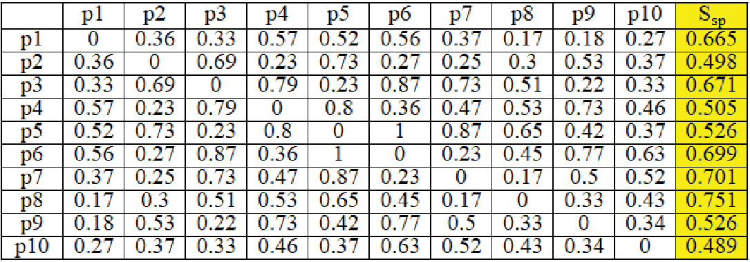
Now, we will calculate the socio-spatial relevance score and socio-spatial diversity of the locations considering equal weight in social and spatial factors, e.g., . Therefore, we calculate the socio-spatial relevance score of as . Similarly, the socio-spatial diversity is calculated as . The Table in Figure 4 shows the socio-spatial relevance scores () and diversity of ’s locations calculated using . Note, we only need to pre-compute the socio-spatial relevance of the locations. We consider in the SSLS query.

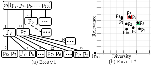
Figure 5 illustrates the node exploration towards searching for the top- SSLS locations. Each state (node in tree) is marked with a number denoting the node exploration sequence. A priority queue, is initialized with and , where contains ’s locations in non-increasing order of relevance scores (). The entries (Algorithm 1, Line 1) and (Line 1) are pushed to for further exploration. Next, is dequeued from . We begin exploring from , and becomes (step ). In the meantime, is pushed to (Line 1), and we get the first feasible solution with . Continuing the process (till step ), the best feasible set with is obtained in this branch.
Further, we dequeue and explore the branch with node (Step ). After processing lines 1 and 1 of Algorithm 1, we check pruning condition at Line 1 using Property 2, where is computed using Equation 9. As, is true w.r.t. each location in current , we continue exploring the branch with node and update the best feasible set as with . In the next iteration while exploring node (step20), we calculate w.r.t. and . All the locations in satisfy Property 2, therefore, we terminate processing . By exploring the remaining branches, we obtain as the top- SSLS set for the query user .
V An Approximate Approach
One major limitation of Exact approach is the high computational cost, which makes it unrealistic for a large number of candidate locations. To validate the location pruning in Exact, it is required to calculate the updated diversity of the current intermediate set w.r.t. each location . Calculating for each intermediate set is expensive when the size of is large.
Therefore, to improve pruning and advanced termination, we derive relaxed bounds on diversity. We first define the maximum possible score of for an intermediate set when an eligible location is added to . Lemma 1 deduces is true for any intermediate set . Therefore, the maximum possible value of can be obtained as,
| (10) |
Note that is dependent on , and is true w.r.t. only when strictly holds. Therefore, to make an efficient approximate approach, we design pruning and termination in the below subsection using lower bound on . We consider always true w.r.t. each location .
Computing bounds on diversity of locations. Let us consider be an intermediate set of size , be an eligible location, and be the best feasible set identified already. For an arbitrary eligible location that can be added to , we continue to derive Equation 7,
We will first derive a relaxed bound for termination using the above equation. Therefore, we replace the upper bound of with its maximum possible value, e.g., ,
Now, we will generalize the above condition for any intermediate set of size . So, we need to add an arbitrary subset to such that . Hence,
Next, we will derive the lower bound by replacing the expression with the total socio-spatial relevance score of top relevant locations from . We calculate the total socio-spatial relevance score of the top locations as . Hence, we get the lower bound of as follows,
| (11) |
Pruning and Termination Rules. We terminate processing an intermediate set when , is true. This is because, there exists no location in that can form a better set containing than the best feasible set . Otherwise, we need to prune the particular locations that satisfy . As we consider, is always true for an intermediate set regardless of , the derived lower bound may produce the answer set to miss some eligible locations. Nevertheless, the approach achieves high efficiency with the sacrifice of a certain precision.
Algorithm. For our Approximate (AP) solution, we modify the Exact algorithm to introduce the advanced termination and pruning as described above. Here, we only need to replace the methods at Line 1 in Algorithm 1 using the above mentioned termination and pruning rules based on when an intermediate set contains more than one location. The time complexity of AP is similar to Exact, as both the algorithms execute same number of iterations in worst case.
Approximation Ratio. We derive a theoretical bound on the approximation ratio of our Approximate approach (AP). We define the ratio as the socio-spatial score of the SSLS set returned by Exact algorithm divided by the score of the AP. Let’s assume, be the approximate set, and be the exact solution of size , where locations are added progressively to and to . To accelerate the Approximate approach, we had derived a relaxed lower bound considering is always true (refer Section V). This means, AP will discard some eligible locations , whose diversities (w.r.t. an intermediate set ) lie between . Let, produces maximum socio-spatial score w.r.t. the intermediate set, therefore, will be part of the exact solution . Similarly, let produces the maximum socio-spatial score among the locations whose diversity w.r.t. is more than , e.g., . Hence, , and will be part of the approximate solution. Therefore, is true, and we derive, , where is the difference in the diversity of the locations and w.r.t. corresponding intermediate set (e.g., ).
Following the above process, let’s assume that we find the exact set and the approximate solution arranged in decreasing order of relevance score, and . As we progressively add the locations, each time the lower bound gets update. We assign as the minimum score among the lower bounds we derived at each step. Therefore, the lowest total diversity of will be , and the socio-spatial score of the lowest scoring approximate set is . Similarly, for the exact set, we calculate the best total diversity score as , where the diversity of each location is slightly smaller by than . Also, we calculate the best total relevance score . Let , therefore, . Hence, the approximation ratio will be bounded by:
Let us assume, , s.t., . Now, if we emphasize on higher diversity (e.g., ), the approximation ratio will be , while, it returns when emphasize on the relevance (e.g., ).
VI A Fast Exact Algorithm
The socio-spatial diversity of a location is dependent on the other locations in a set. The pruning strategies based on the bound derived by diversity need to re-calculate the diversity scores of the locations whenever the intermediate set gets an update. Therefore, the algorithms based on the bound derived by diversity (e.g., Exact) consume more time to execute. In this section, we develop an efficient exact method (Exact+) that considers bounds on the relevance scores of the candidate locations. Such a practice will help to search the exact results by reducing the complex diversity computation of intermediate sets (as performed in Exact). The key idea of Exact+ is motivated by the following observations: (i) As the relevance score of each member in a set is independent of the other members; it will be computationally efficient to design pruning strategies on relevance scores. (ii) Lemma 2 suggests that a location with a relevance score more than is eligible to be added to an intermediate set. Therefore, we can easily derive a lower bound on relevance score using the above observations to prune a large number of irrelevant locations.
VI-A Computing Bounds on Relevance
Here, we introduce some lemmas to derive bounds for pruning locations and early termination. The below lemma aims to compute the maximum possible socio-spatial diversity of a set when an arbitrary location is added to an intermediate result set .
Lemma 4 (Maximum Socio-spatial Diversity of an Updated Intermediate Set).
Given an intermediate set , an arbitrary location , the maximum Socio-spatial diversity of an updated set will be , where is the maximum diversity generated by an arbitrary location of w.r.t. .
Proof.
Now, we will derive the lower bound for the socio-spatial relevance score (). Such bound will identify the locations that can be added to the current intermediate set. Meanwhile, we label the reference location () that has maximum socio-spatial relevance score among the remaining locations in .
Lemma 5 (Lower Bound of Relevance Score).
Given an intermediate set , reference location , and the remaining location set , the lower bound of Socio-Spatial Relevance Score is , where is the maximum diversity of locations in w.r.t. .
Proof.
Suppose the reference location has been added to the intermediate set , the socio-spatial score of the updated intermediate set can be computed as,
Given another location s.t. , it needs to be probed only when according to the selection criteria. Hence, we simplify the condition below.
Now, we substitute with its maximum value using Lemma 4. Therefore, we get . ∎
If contains single location, we compute the lower bound as , as if . Now, using Lemma 5, we identify the potential locations that can be added to the current intermediate set.
Property 3 (Potential Locations).
A location is a potential candidate location w.r.t. if .
VI-B Advanced Termination
The Exact+ algorithm needs to iteratively check the remaining locations until the best result set is determined. However, it is time-consuming to process all intermediate sets and checks for the feasible set at each iteration. Therefore, we need to introduce some lemmas to derive early termination criteria. First, similar to Lemma 4, we derive below lemma on maximum possible socio-spatial diversity of an answer set.
Lemma 6 (Maximum Socio-spatial Diversity of an Answer Set).
Given set , an arbitrary subset of locations of size s.t., and ; the maximum Socio-spatial diversity of the set is , where is the sum of the top socio-spatial diversity scores of the locations w.r.t. .
Proof.
Proof is omitted due to space limitations. ∎
For any intermediate set and a feasible solution of size containing , s.t. , we derive the below lemma on maximum possible socio-spatial score of .
Lemma 7 (Maximum Socio-spatial Score of an Answer Set).
Given an intermediate set , an arbitrary subset of locations of size s.t., , the maximum possible socio-spatial score of is , where, is the sum of top socio-spatial relevance scores of the remaining set , s.t., and .
Proof.
Let an arbitrary location set of size is added to s.t. . The socio-spatial score of is,
| (12) |
To achieve the maximum socio-spatial score of , we need to replace the two unknown variables and in Equation 12 with their maximum possible scores.
Property 4 (Advanced Termination).
Given an intermediate set , a -sized answer set , and the best feasible set , if , we will terminate processing .
The Exact+ algorithm incrementally adds locations and checks for a feasible set. It prunes some locations using the lower bound on relevance score, and further terminates processing large number of intermediate sets using Property 4.
VI-C Algorithm
Algorithm 2 summarizes the major steps of Exact+, for processing the SSLS query. Given a socio-spatial graph , query user , the top- SSLS query returns a set of size . Initially, the locations of user are added to in non-increasing order of their relevance scores and marked as unvisited. In each iteration, the unvisited locations of are copied to , and the top relevant location of is added to (Line 2). Further, the advanced termination of the current intermediate set is probed using Property 4 (Line 2). In Line 2, the lower bound on relevance score () is calculated using Lemma 5, and the potential locations () are identified using Property 3 (Line 2). The intermediate set is updated with the location that generates maximum socio-spatial score (Line 2). The inner loop continues until a set of locations is found, and finally, it returns the best set .
19
Time Complexity. The worst case time complexity of Exact+ algorithm is , where is the number of locations of a user. The outer loop and inner loop take and , respectively. The complexity of other major parts are: process in , selection in , computation in , selection in , and selection in .
Steps of Exact+. We use the example in Figure 1 to demonstrate the steps of Exact+ (Algorithm 2) for selecting top- SSLS set for user . We show the node exploration steps of the first iteration of Exact+ in Figure 5 (b). The calculated relevance and diversity scores of the locations are available in Figure 4. We set the trade-off parameters as , .
First, we add ’s locations in in non-increasing score. Next, the top relevant location (shown in left bottom corner of Figure 5 (b)) is added to intermediate set . As the termination condition is not satisfied at Line 2, we process to explore the remaining locations in . First, we select the reference location as (Line 2) shown within red box in Figure 5 (b), and the remaining locations in are shown as black dots. The Y and X axes denote the relevance scores and diversity of the locations in w.r.t. , respectively. Now, the lower bound in relevance score w.r.t. is calculated using Lemma 5, e.g., . The horizontal line in red depicts the lower bound in relevance score. The points on or above the line are labeled as potential locations (), and are pruned w.r.t. intermediate set . The location (marked in green box) among produces the maximum score (Line 2). Therefore, in this iteration, we get the best set of locations as . The process continues until no unvisited locations exist in . We finally get as the top- SSLS solution for with socio-spatial score .
Fast Approximate. From our empirical evaluation, we find that greedily selecting the best locations using Exact+, the results rapidly converge towards an optimal solution in the first few iterations. To make a reasonable trade-off between performance and accuracy, we consider an early termination of Exact+ after two iterations in our Fast Approximate (FA) algorithm. In Figure 1, FA will select for user considering the first two iterations of Exact+.
VII Experimental Evaluation
In this section, we present the experimental evaluation of our proposed approaches for Top- SSLS queries: the Exact solution (E); the Approximate solution (AP); the Exact+ solution (EP); and the Fast Approximate solution (FA). We implement the algorithms using Python 3.6 on Windows environment with 3.40GHz CPU and 64GB RAM. To further validate, we compared with three baselines adapted from existing works:
GMC [6]. It combines relevance and diversity, and greedily selects the elements based on their marginal contributions. Locations with the highest partial contributions will be selected.
Adaptive-SOS [5]. To make the adaption of SSLS to SOS [5], denoted as AS, we model the social similarity of a pair of locations by using their common users who checked in the location pair. Thus, an edge can be added between the two locations if the similarity is more than a threshold (e.g., 0.4).
GNE [6]. It randomly adds a location from the top ranked locations into a temporary result set. Then, it performs swaps between elements of the temporary result set and the most diverse elements of the candidate set.
| Data | Users | Edges | Checkins | Places | AC | AF | AFC |
| GW | 107,092 | 456,830 | 6,442,892 | 1,280,969 | 60 | 8.5 | 4.6 |
| BK | 51,405 | 214,078 | 4,491,143 | 772,783 | 87 | 7.7 | 3.8 |
| FL | 189,537 | 2,028,873 | 12,592,819 | 4,896,634 | 66 | 21.4 | 0.3 |
| YL | 270,323 | 1,913,501 | 5,425,778 | 192,609 | 20 | 14.2 | 10.4 |
Datasets. We conduct experiments using four real-world large datasets: Gowalla (GW), Brightkite (BK), Flickr (FL), and Yelp (YL). Gowalla [39] and Brightkite [39], each contains the social connections of the users, and the check-ins available over the period Feb. 2009 - Oct. 2010 and Apr. 2008 - Oct. 2010 respectively. Flickr data was collected using Flickr public API in 2017-18. We establish a social link between a user pair using the following information, and consider a check-in if a user has a photo geo-tagged the location. Yelp (collected from https://www.yelp.com/dataset/, Round 13, Year 2019) contains friendship network and POIs of users in the form of reviews, and location-tags in users’ tips. Table II presents brief statistics of the four datasets, where the last three columns show the Average Check-ins (AC) by users, Average Friendships (AF), and Average number of Friends that users have at places they have Checked-in (AFC). In Figure 6, we show the number of users have friends in the given ranges, where the x-axis labels ‘100’, ‘200’, ‘500’, ‘1K’ , ‘1K’ denote the number of friends in the ranges ‘10-100’, ‘101-200’, ‘201-500’, ‘501-1K’, and ‘K’ respectively.


Figure 7 shows the check-in characteristics of the users in different check-in ranges.


Evaluation Metrics. It represents the percentage of the common elements (e.g., locations) between the result set returned by an approach and the exact results.
Likewise, Minimization of the Mean of Shortest Distance (MMSD) [40, 41], we calculate the Mean of Minimum Diversity (MMD) for a query user w.r.t. neighbors’ locations, i.e., . This metric shows how well the selected set of locations for user can cover her friends . Note, in a socio-spatial domain, is considered as socio-spatial distance () between two locations.
To measure the social quality of the selected set, we compute social coverage using the percentage of friends who have at least one check-in within kilometer (KM) from the selected set , i.e., .
Given a selected set of locations of , let be the set of ’s friends who visits . The social entropy of the set of is, , where, . SE measures the diversity of a location set w.r.t. the participation of its users across different other groups [36]. Here, for a selected location of , one of ’s corresponding group is considered as the friends who visited (e.g. ). A higher social entropy of a set suggests that the selected locations can cover more socially diverse friends.
| Parameter | Values | Default |
|---|---|---|
| Check-in group id |
Parameter Configuration. Table III presents the varied range of the parameters with default values. If there is no specific declaration, then the default values of the parameters will be used when one parameter varies. We only consider users having at least ten check-ins and at least two friends with check-in information. To see the effect of varying number of check-ins, we divide the users of each dataset into five groups based on the number of location check-ins they have. The group ids 50, 100, 200, 500, and 1000 contain the users with check-in locations in the range 10-50, 51-100, 101-200, 201-500, and 501-1000, respectively.
VII-A Efficiency Evaluation
In this section, we compare the scalability of our proposed approaches.
VII-A1 Varying Answer Set Size,
Figure 8 shows the average runtime of our proposed methods by varying between 2 to 10. The runtime of the algorithms follow similar trends, where E consumes maximum time to process a query. On average, EP is 2 to 3 times faster than AP, and 3 to 6 times faster than E. We notice, AP performs efficiently than EP for those users who have candidate locations with similar relevance scores, and higher diversity. Also, AP is three times faster than E and FA is 9 to 15 times faster than EP in different datasets when varies from 2 to 10.


VII-A2 Varying Check-in Group Size
In this experiment, we study the performance of the proposed approaches on the distribution of number of check-ins. Specifically, we show how the size of the check-in locations (e.g., candidate set) of users affects the performance on the approaches. From Figure 9, we find the runtime of the proposed approaches, except FA, increases fast with the check-in group size. This is because a considerable amount of possible groups of locations are needed to compare in E, AP, and EP when the check-in group size is large. We also notice EP is much efficient than E and AP. For example, in check-in group 500 in Brightkite, EP reports 2.5 and 4.7 times faster than AP and E, respectively. FA performs significantly efficient, even for the large candidate set. For example, in Gowalla, FA is 57 times faster than EP when the check-in group id is 1000.


VII-A3 Varying Number of Friends
We compare the efficiency of our proposed algorithms by varying the number of social connections users have. To balance user count with sufficient check-ins, we first select the check-in group 500, then divide the users into five groups with medium to a higher number of social connections. The user group ids 100, 200, 500, 1000 contain the users with 50-100, 101-200, 201-501, 501-1000 friends, respectively. In Figure 10, we notice a similar trend in the proposed methods, where a higher number of friends do not affect the efficiency. This is because, the social and spatial relevance scores are pre-computed using the location information of the friends. The proposed algorithms only depend on the number of check-ins a query user has. Therefore, it merely gets affected by the number of social connections.


VII-A4 Varying , and
We also test our proposed algorithms by varying the trade-off parameters , . Figure 11 shows the average runtime of our proposed algorithms in Gowalla and Yelp datasets when the trade-off parameters , vary from to . As expected, we do not observe any noticeable change in the efficiency trends in each datasets, where the average execution time of individual algorithm almost remains constant. This is because, these trade-off parameters do not interfere on how a method operates, but only precepts in selecting locations in the result set.


VII-B Comparison with Existing Models
We compare the performance of the existing greedy solutions, e.g., GMC, AS, GNE, with our proposed approaches. For brevity of the presentation, we only show the results using the medium-sized dataset Gowalla and the large dataset Yelp.
VII-B1 Efficiency
To make a fair comparison between the greedy based existing works and our proposed solutions, we consider our top two efficient algorithms, EP and FA, in this experiment. Figure 12 depicts the runtime of the approaches by varying the answer set size in default check-in group. In Gowalla dataset, GNE has higher efficiency than EP, but in Yelp, it shows an opposite trend. This is because the candidate locations in check-in group 100 of Yelp is higher than Gowalla. GNE always performs slower than FA; e.g., in Yelp, GNE is two times slower than FA. In each dataset with moderate-sized candidate locations, GMC performs faster than the others.


Figure 13 compares the runtime of the approaches when check-in group size varies. We notice that FA is faster than GMC when the check-in group size is more than 100. This is because, GMC needs more time to calculate the marginal contribution of the locations in large candidate sets. In higher check-in groups, GNE takes considerable time to swap the locations in the current result set and the most diverse element among the remaining locations which results a lower efficiency.


VII-B2 Accuracy
Figure 14 demonstrates the precision of the approaches w.r.t. the exact result when is varied. AP has higher precision than the other approaches in each dataset. Although the precision of FA is lower than AP, FA is much efficient (e.g., 10-25 times faster, see Figure 8). For example, in Yelp, FA’s precision is lower than AP by 16% only, but its efficiency outperforms AP by about 20 times when .


Figure 15 shows the average precision of the models when and vary. As the relative trends are similar on other datasets, we only show the effect of and on Gowalla. The precision of the methods typically increases with (e.g., preference to relevance). The FA and AS methods are influenced by the selection of top relevant location in the result set, which affects the precision when diversity has higher importance than relevance. The precision of AP, GMC, and GNE remain almost constant when varies. The variation of does not affect much in the precision of the approaches when is set as default. For example, in Gowalla, the average precision of AP is when varies and . In Yelp, the average precision of AP is reported as 68% when varies from to .


VII-B3 Effectiveness
We compare the socio-spatial qualities of the selected locations using the MMD metric. In Gowalla (Figure 16(a)), the MMD of AS remains almost constant, while for the other approaches, the MMD score decreases smoothly with the increase of . This is because the AS model considers a fixed user-defined threshold to maintain a minimum diversity. In Yelp, all the approaches produce lower MMD (Figure 16(b)). This means the majority of user’s friends in Yelp have closer check-ins to the selected locations.


Figure 17 compares the social coverage (SC) of the algorithms. In both the datasets, the relative trends are similar. The top- locations in EP are co-located with 64% and 74% neighbors in Gowalla and Yelp datasets, respectively. The GMC method has the lowest SC, i.e., it reports only 30% in Yelp. Interestingly, we find that the social coverage of FA is marginally higher than EP. This is because, FA includes the top socio-spatial relevant locations in the result set. Therefore, the selected set has exact check-ins by a large number of friends.


Figure 18 shows the average social entropy (SE) of the approaches when answer set size varies. Similar trends are followed in both the datasets. The EP approach has the highest average SE, which means the selected locations by EP have diverse participation of friends. Meanwhile, EP also has higher social coverage (SC) (Figure 17). These two metrics SE and SC together establish that the selected locations in EP not only cover a large number of friends, but represent diverse groups. Compared with GMC and GNE, AS has higher social entropy.


VII-B4 Memory Consumption
We observe that EP, FA, GMC, GNE, AS has similar memory consumption, where the average memory usages are reported as 1195MB, 845MB, 2940MB, 1410MB on Gowalla, Brightkite, Flickr, and Yelp, respectively. The Exact and AP methods need to store the intermediate set information in a priority queue, which leads to higher memory cost. For example, in Brightkite, and consume average 1150MB for the users in check-in group 100.
VII-C A Case Study on Location Set Selection
In Figure 19, we visualize the selection result of top- SSLS using Adaptive SOS, Exact, and Approximate methods considering , . First, we choose a query user (userid ‘10’) from Gowalla [39] dataset, and select the region (38.85, -94.85) to (39.11, -94.58) on map where the user has majority of its check-ins. Further, we obtain the check-in information of the neighbors of the user ‘10’ having at least ten check-in in the mentioned area. There are nine such neighbors available in the selected region. Locations of the user ‘10’ and its neighbors are marked in yellow and blue, respectively (best visible in color with zooming). The user ‘10’ has frequent check-ins concentrated at the red bordered region shown in Figure 19(a). The five locations selected by the Adaptive SOS (AS) model are quite distant (shown in red icons in Figure 19(a)). However, AS has ignored one important location (39.10, -94.59) (marked as red at NE corner in Figure 19(b)) which is included in top- SSLS result by our proposed Exact and Approximate approaches. This location (39.10, -94.59) is spatially relevant to the user ‘10’, as six neighbors (out of nine) have multiple check-ins (total 62) in 7 nearby places within . In such a configuration, our Approximate approach has four common selection as Exact. Meanwhile, we provide the snippet of the socio-spatial information of the user ‘10’ (of Gowalla dataset) and its neighbors (who had at least check-ins at the region (38.85, -94.85) to (39.11, -94.58)) at https://github.com/nurjamia/SSLS/blob/master/CaseStydyUserid10_GW.txt.


VIII Conclusion
In this paper, we propose a novel problem of identifying top-k Socio-Spatial co-engaged Location Selection. It selects locations for a user from a large number of candidate locations based on the dominance of the combined socio-spatial diversity and relevance scores. We develop two exact and two approximate solutions to solve this NP-hard problem. Finally, the quality of our proposed approaches has been validated by comparing with the state-of-the-art object selection models. The extensive experimental studies on four real datasets with various socio-spatial characteristics have verified the performance of our proposed approaches.
References
- [1] I. Konstas, V. Stathopoulos, and J. M. Jose, “On social networks and collaborative recommendation,” in Proceedings of ACM SIGIR, 2009, pp. 195–202.
- [2] M. Ye, P. Yin, and W.-C. Lee, “Location recommendation for location-based social networks,” in Proceedings of SIGSPATIAL GIS, 2010, pp. 458–461.
- [3] M. Ye, P. Yin, W.-C. Lee, and D.-L. Lee, “Exploiting geographical influence for collaborative point-of-interest recommendation,” in ACM SIGIR, 2011, pp. 325–334.
- [4] M. Drosou and E. Pitoura, “Disc diversity: result diversification based on dissimilarity and coverage,” Proceedings of the VLDB Endowment, vol. 6, no. 1, pp. 13–24, 2012.
- [5] T. Guo, K. Feng, G. Cong, and Z. Bao, “Efficient selection of geospatial data on maps for interactive and visualized exploration,” in ACM SIGMOD. ACM, 2018, pp. 567–582.
- [6] M. R. Vieira, H. L. Razente, M. C. Barioni, M. Hadjieleftheriou, D. Srivastava, C. Traina, and V. J. Tsotras, “On query result diversification,” in ICDE. IEEE, 2011, pp. 1163–1174.
- [7] N. Armenatzoglou, S. Papadopoulos, and D. Papadias, “A general framework for geo-social query processing,” Proceedings of the VLDB Endowment, vol. 6, no. 10, pp. 913–924, 2013.
- [8] A. Sohail, M. A. Cheema, and D. Taniar, “Geo-social temporal top-k queries in location-based social networks,” in ADC. Springer, 2020, pp. 147–160.
- [9] B. Ghosh, M. E. Ali, F. M. Choudhury, S. H. Apon, T. Sellis, and J. Li, “The flexible socio spatial group queries,” Proceedings of the VLDB Endowment, vol. 12, no. 2, pp. 99–111, 2018.
- [10] A. Sohail, G. Murtaza, and D. Taniar, “Retrieving top-k famous places in location-based social networks,” in ADC. Springer, 2016, pp. 17–30.
- [11] N. A. H. Haldar, J. Li, M. Reynolds, T. Sellis, and J. X. Yu, “Location prediction in large-scale social networks: an in-depth benchmarking study,” The VLDB Journal, pp. 1–26, 2019.
- [12] R. Li, S. Wang, and K. C.-C. Chang, “Multiple location profiling for users and relationships from social network and content,” Proceedings of the VLDB, vol. 5, no. 11, pp. 1603–1614, 2012.
- [13] R. Li, S. Wang, H. Deng, R. Wang, and K. C.-C. Chang, “Towards social user profiling: unified and discriminative influence model for inferring home locations,” in Proceedings of the 18th ACM SIGKDD. ACM, 2012, pp. 1023–1031.
- [14] J. Bao, Y. Zheng, and M. F. Mokbel, “Location-based and preference-aware recommendation using sparse geo-social networking data,” in SIGSPATIAL GIS, 2012, pp. 199–208.
- [15] Y. Zheng, L. Zhang, Z. Ma, X. Xie, and W.-Y. Ma, “Recommending friends and locations based on individual location history,” ACM TWEB, vol. 5, no. 1, pp. 1–44, 2011.
- [16] I. Catallo, E. Ciceri, P. Fraternali, D. Martinenghi, and M. Tagliasacchi, “Top-k diversity queries over bounded regions,” ACM TODS, vol. 38, no. 2, p. 10, 2013.
- [17] M. Drosou and E. Pitoura, “Diverse set selection over dynamic data,” IEEE TKDE, vol. 26, no. 5, pp. 1102–1116, 2014.
- [18] P. Fraternali, D. Martinenghi, and M. Tagliasacchi, “Top-k bounded diversification,” in ACM SIGMOD. ACM, 2012, pp. 421–432.
- [19] L. Qin, J. X. Yu, and L. Chang, “Diversifying top-k results,” Proceedings of VLDB Endowment, vol. 5, no. 11, pp. 1124–1135, 2012.
- [20] A. Angel and N. Koudas, “Efficient diversity-aware search,” in Proceedings of ACM SIGMOD. ACM, 2011, pp. 781–792.
- [21] X. Zhu, J. Guo, X. Cheng, P. Du, and H.-W. Shen, “A unified framework for recommending diverse and relevant queries,” in Proceedings of WWW, 2011, pp. 37–46.
- [22] C.-N. Ziegler, S. M. McNee, J. A. Konstan, and G. Lausen, “Improving recommendation lists through topic diversification,” in Proceedings of WWW. ACM, 2005, pp. 22–32.
- [23] C. L. Clarke, M. Kolla, G. V. Cormack, O. Vechtomova, A. Ashkan, S. Buttcher, and I. MacKinnon, “Novelty and diversity in information retrieval evaluation,” in Proceedings of ACM SIGIR. ACM, 2008, pp. 659–666.
- [24] R. Agrawal, S. Gollapudi, A. Halverson, and S. Ieong, “Diversifying search results,” in ACM WSDM, 2009, pp. 5–14.
- [25] A. Borodin, H. C. Lee, and Y. Ye, “Max-sum diversification, monotone submodular functions and dynamic updates,” in Proceedings of PODS, 2012, pp. 155–166.
- [26] S. Gollapudi and A. Sharma, “An axiomatic approach for result diversification,” in WWW, 2009, pp. 381–390.
- [27] J. Carbonell and J. Goldstein, “The use of mmr, diversity-based reranking for reordering documents and producing summaries,” in Proceedings of the 21st ACM SIGIR, 1998, pp. 335–336.
- [28] M. Drosou and E. Pitoura, “Diversity over continuous data.” IEEE Data Eng. Bull., vol. 32, no. 4, pp. 49–56, 2009.
- [29] E. Elhamifar and M. Clara De Paolis Kaluza, “Online summarization via submodular and convex optimization,” in Proceedings of IEEE CVPR, 2017, pp. 1783–1791.
- [30] Q. Zhou, N. Yang, F. Wei, S. Huang, M. Zhou, and T. Zhao, “Neural document summarization by jointly learning to score and select sentences,” arXiv preprint arXiv:1807.02305, 2018.
- [31] A. Das Sarma, H. Lee, H. Gonzalez, J. Madhavan, and A. Halevy, “Efficient spatial sampling of large geographical tables,” in ACM SIGMOD. ACM, 2012, pp. 193–204.
- [32] S. Nutanong, M. D. Adelfio, and H. Samet, “Multiresolution select-distinct queries on large geographic point sets,” in Proceedings ACM SIGSPATIAL GIS, 2012, pp. 159–168.
- [33] M. Mahdian, O. Schrijvers, and S. Vassilvitskii, “Algorithmic cartography: Placing points of interest and ads on maps,” in Proceedings of ACM SIGKDD. ACM, 2015, pp. 755–764.
- [34] F. Wang, G. Wang, and S. Y. Philip, “Why checkins: Exploring user motivation on location based social networks,” in ICDMW. IEEE, 2014, pp. 27–34.
- [35] N. Armenatzoglou, R. Ahuja, and D. Papadias, “Geo-social ranking: functions and query processing,” The VLDB Journal, vol. 24, no. 6, pp. 783–799, 2015.
- [36] J. Shi, N. Mamoulis, D. Wu, and D. W. Cheung, “Density-based place clustering in geo-social networks,” in Proceedings of ACM SIGMOD. ACM, 2014, pp. 99–110.
- [37] J. Su, K. Kamath, A. Sharma, J. Ugander, and S. Goel, “An experimental study of structural diversity in social networks,” arXiv preprint arXiv:1909.03543, 2019.
- [38] M. R. Garey and D. S. Johnson, Computers and intractability. wh freeman New York, 2002, vol. 29.
- [39] J. Leskovec and A. Krevl, “Snap datasets: Stanford large network dataset collection,” http://snap.stanford.edu/data, June 2014.
- [40] E. M. Delmelle, “Spatial sampling,” Handbook of regional science, pp. 1385–1399, 2014.
- [41] J.-F. Wang, A. Stein, B.-B. Gao, and Y. Ge, “A review of spatial sampling,” Spatial Statistics, vol. 2, pp. 1–14, 2012.