We are grateful for useful discussions to Lokman Abbas-Turki, Agostino Capponi, Karl-Theodor Eisele, Chris Kenyon, Marek Rutkowski, and Michael Schmutz. The PhD thesis of Bouazza Saadeddine is funded by a CIFRE grant from CA-CIB and French ANRT. ††footnotetext: Disclaimers: The views expressed herein by Rodney Hoskinson and co-authors are their personal views and do not reflect the views of ANZ Banking Group Limited (”ANZ”). No liability shall be accepted by ANZ whatsoever for any direct or consequential loss from any use of this paper and the information, opinions and materials contained herein.††footnotetext: Email addresses: claudio.albanese@global-valuation.com, stephane.crepey@univ-evry.fr, rodney.hoskinson@edhec.com, bouazza.saadeddine@univ-evry.fr
XVA Analysis From the Balance Sheet
Abstract
XVAs denote various counterparty risk related valuation adjustments that are applied to financial derivatives since the 2007–09 crisis. We root a cost-of-capital XVA strategy in a balance sheet perspective which is key in identifying the economic meaning of the XVA terms. Our approach is first detailed in a static setup that is solved explicitly. It is then plugged in the dynamic and trade incremental context of a real derivative banking portfolio. The corresponding cost-of-capital XVA strategy ensures to bank shareholders a submartingale equity process corresponding to a target hurdle rate on their capital at risk, consistently between and throughout deals. Set on a forward/backward SDE formulation, this strategy can be solved efficiently using GPU computing combined with deep learning regression methods in a whole bank balance sheet context. A numerical case study emphasizes the workability and added value of the ensuing pathwise XVA computations.
Keywords: Counterparty risk, balance sheet of a bank, market incompleteness, wealth transfer, X-valuation adjustment (XVA), deep learning, quantile regression.
Mathematics Subject Classification:
91B25, 91B26, 91B30, 91G20, 91G40, 62G08, 68Q32.
JEL Classification: D52, G13, G24, G28, G33, M41.
1 Introduction
XVAs, with X as C for credit, D for debt, F for funding, M for margin, or K for capital, are post-2007–09 crisis valuation adjustments for financial derivatives. In broad terms to be detailed later in the paper (cf. Table 1 in Section 2), CVA is what the bank expects to lose due to counterparty defaults in the future; DVA (irrelevant for pricing but material to bank creditors as we will see) is what the bank expects to gain due to its own default; FVA is the expected cost for the bank of having to raise variation margin (re-hypothecable collateral) ; MVA is the expected cost for the bank of having to raise initial margin (segregated collateral); KVA is the expected cost for the bank of having to remunerate its shareholders through dividends for their capital at risk.
XVAs deeply affect the derivative pricing task by making it global, nonlinear, and entity dependent. However, before these technical implications, the fundamental point is to understand what really deserves to be priced and what does not, by rooting the pricing approach in a corresponding collateralization, accounting, and dividend policy of the bank.
Coming after several papers on the valuation of defaultable assets in the 90’s, such as ?), ?, Eq. (14.25) p. 448) obtained the formula
| (1) |
for the valuation of bilateral counterparty risk on a swap, assuming risk-free funding. This formula, rediscovered and generalized by others since the 2008–09 financial crisis (cf. e.g. ?)), is symmetrical, i.e. it is the negative of the analogous quantity considered from the point of view of the counterparty, consistent with the law of one price and the ?) theorem.
Around 2010, the materiality of the DVA windfall benefit of a bank at its own default time became the topic of intense debates in the quant and academic communities. At least, it seemed reasonable to admit that, if the own default risk of the bank was accounted for in the modeling, in the form of a DVA benefit, then the cost of funding (FVA) implication of this risk should be included as well, leading to the modified formula (). See for instance [Burgard and Kjaer (2011] (?, ?, ?), ?), ?), or ?). See also ?) for an abstract funding framework (without explicit reference to XVAs), generalizing ?) to a nonlinear setup.
Then ?) objected that the FVA was only the compensator of another windfall benefit of the bank at its own default, corresponding to the non-reimbursement by the bank of its funding debt. Accounting for the corresponding “DVA2” (akin to the FDA in this paper) brings back to the original firm valuation formula:
as (assuming risky funding fairly priced as we will see).
However, their argument implicitly assumes that the bank can perfectly hedge its own default: cf. ?, end of Section 3.1) and see Section 3.5 below. As a bank is an intrinsically leveraged entity, this is not the case in practice. One can mention the related corporate finance notion of debt overhang in ?), by which a project valuable for the firm as a whole may be rejected by shareholders because the project is mainly valuable to bondholders. But, until recently, such considerations were hardly considered in the field of derivative pricing.
The first ones to recast the XVA debate in the perspective of the balance sheet of the bank were ?), to explain that an appropriately hedged derivative position has no impact on the dealer’s funding costs. Also relying on balance sheet models of a dealer bank, ?) and ?) end up with conflicting conclusions, namely that the FVA should, respectively should not, be included in the valuation of financial derivatives. Adding the KVA, but in a replication framework, ?) conclude that both the FVA and the KVA should be included as add-ons in entry prices and as liabilities in the balance sheet.
1.1 Contents
Our key premise is that counterparty risk entails two distinct but intertwined sources of market incompleteness:
- •
A bank cannot perfectly hedge counterparty default losses, by lack of sufficiently liquid CDS markets;
- •
A bank can even less hedge its own jump-to-default exposure, because this would mean selling protection on its own default, which is nonpractical and, under certain juridictions, even legally forbidden (see Section 2).
We specify the banking XVA metrics that align derivative entry prices to shareholder interest, given this impossibility for a bank to replicate the jump-to-default related cash flows. We develop a cost-of-capital XVA approach consistent with the accounting standards set out in IFRS 4 Phase II (see ?)), inspired from the Swiss solvency test and Solvency II insurance regulatory frameworks (see ?) and ?)), which so far has no analogue in the banking domain. Under this approach, the valuation (CL) of the so-called contra-liabilities and the cost of capital (KVA) are sourced from clients at trade inceptions, on top of the () complete market valuation of counterparty risk, in order to compensate bank shareholders for wealth transfer and risk on their capital.
The cost of the corresponding collateralization, accounting, and dividend policy is, by contrast with the complete market valuation () of counterparty risk,
| (2) |
computed unilaterally in a certain sense (even though we do crucially include the default of the bank itself in our modeling), and charged to clients on an incremental run-off basis at every new deal11 1 See also Remark 2.1 regarding the meaning of the FVA in (2)..
All in one, our cost-of-capital XVA strategy makes shareholder equity a submartingale with drift corresponding to a hurdle rate on shareholder capital at risk, consistently between and throughout deals. Thus we arrive at a sustainable strategy for profits retention, much like in the above-mentioned insurance regulation, but in a consistent continuous-time and banking framework.
Last but not least, our approach can be solved efficiently using GPU computing combined with deep learning regression methods in a whole bank balance sheet context.
1.2 Outline and Contributions
Section 2 sets a financial stage where a bank is split across several trading desks and entails different stakeholders. Section 3 develops our cost-of-capital XVA approach in a one-period static setup. Section 4 revisits the approach at the dynamic and trade incremental level. Section 5 is a numerical case study on large, multi-counterparty portfolios of interest rate swaps, based on the continuous-time XVA equations for bilateral trade portfolios recalled in Section A.
The main contributions of the paper are:
- •
The one-period static XVA model of Section 3, with explicit formulas for all the quantities at hand, offering a concrete grasp on the related wealth transfer and risk premium issues;
- •
Proposition 4.1, which establishes the connections between XVAs and the core equity tier 1 capital of the bank, respectively bank shareholder equity;
- •
Proposition 4.2, which establishes that, under the XVA policy represented by the balance conditions (4) between deals and the counterparty risk add-on (43) throughout deals, bank shareholder equity is a submartingale with drift corresponding to a target hurdle rate on shareholder capital at risk. This perspective solves the puzzle according to which, on the one hand, XVA computations are performed on a run-off portfolio basis, while, on the other hand, they are used for computing pricing add-ons to new deals;
- •
The XVA deep learning (quantile) regression computational strategy of Section 4.4;
- •
The numerical case study of Section 5, which emphasizes the materiality of refined, pathwise XVA computations, as compared to more simplistic XVA approaches.
From a broader point of view, this paper reflects a shift of paradigm regarding the pricing and risk management of financial derivatives, from hedging to balance sheet optimization, as quantified by relevant XVA metrics. In particular (compare with the last paragraph before Section 1.1), our approach implies that the FVA (and also the MVA, see Remark 2.1) should be included as an add-on in entry prices and as a liability in the balance sheet; the KVA should be included as an add-on in entry prices, but not as a liability in the balance sheet.
From a computational point of view, this paper opens the way to second generation XVA GPU implementation. The first generation consisted of nested Monte Carlo implemented by explicit CUDA programming on GPUs (see ?), ?)). The second generation takes advantage of GPUs leveraging via pre-coded CUDA/AAD deep learning packages that are used for the XVA embedded regression and quantile regression task. Compared to a regulatory capital based KVA approach, an economic capital based KVA approach is then not only conceptually more satisfying, but also simpler to implement.
2 Balance Sheet and Capital Structure Model of the Bank
We consider a dealer bank, which is a market maker involved in bilateral derivative portfolios. For simplicity, we only consider European derivatives. The bank has two kinds of stakeholders, shareholders and bondholders. The shareholders have the control of the bank and are solely responsible for investment decisions before bank default. The bondholders represent the senior creditors of the bank, who have no decision power until bank default, but are protected by laws, of the pari-passu type, forbidding trades that would trigger value away from them to shareholders during the default resolution process of the bank. The bank also has junior creditors, represented in our framework by an external funder, who can lend unsecured to the bank and is assumed to suffer an exogenously given loss-given-default in case of default of the bank.
We consider three kinds of business units within the bank (see Figure 1 for the corresponding picture of the bank balance sheet and refer to Table 1 for a list of the main financial acronyms used in the paper): the CA desks, i.e. the CVA desk and the FVA desk (or Treasury) of the bank, in charge of contra-assets, i.e. of counterparty risk and its funding implications for the bank; the clean desks, who focus on the market risk of the contracts in their respective business lines; the management of the bank, in charge of the dividend release policy of the bank.

| Amounts on dedicated cash accounts of the bank: | ||
| CM | Clean margin | Definition 2.1 and Assumption 2.1 |
| RC | Reserve capital | Definition 2.1 and Assumption 2.1 |
| RM | Risk margin | Definition 2.1 and Assumption 2.1 |
| UC | Uninvested capital | Definition 2.1 and Assumption 2.1 |
| Valuations: | ||
| CA | Contra-assets valuation | (3), (16), and (51) |
| CL | Contra-liabilities valuation | Definition 2.1 and (18), (35), and (43) |
| CVA | Credit valuation adjustment | (17), (16), (52), and (60)–(61) |
| DVA | Debt valuation adjustment | (18) and (17) |
| FDA | Funding debt adjustment | (18) and (23) |
| FV | Firm valuation of counterparty risk | (21) and (23) |
| FVA | Funding valuation adjustment | Remark 2.1, (17), (16), and (52) |
| KVA | Capital valuation adjustment | (4), (26), and (56) |
| MtM | Mark-to-market | (4) and (15) |
| MVA | Margin valuation adjustment | Remark 2.1, (33), (52), and (62) |
| XVA | Generic “X” valuation adjustment | First paragraph |
| Also: | ||
| CR | Capital at risk | (54) |
| CET1 | Core equity tier I capital | (3) and (40) |
| EC | Economic capital | Definitions 3.2 and A.1 |
| FTP | Funds transfer price | (43) |
| SHC | Shareholder capital (or equity) | (3) and (41) |
| SCR | Shareholder capital at risk | Assumption 2.1 and (25) |
Collateral means cash or liquid assets that are posted to guarantee a netted set of transactions against defaults. It comes in two forms: variation margin, which is re-hypothecableotecable, i.e. fungible across netting sets, and initial margin, which is segregated. We assume cash only collateral. Posted collateral is supposed to be remunerated at the risk-free rate (assumed to exist, with overnight index swap rates as a best market proxy).
Remark 2.1
To alleviate the notation, in this conceptual section of the paper, we only consider an FVA as the global cost of raising collateral for the bank, as opposed to a distinction, in the industry and in later sections in the paper, between an FVA, in the strict sense of the cost of raising variation margin, and an MVA for the cost of raising initial margin.
The CA desks guarantee the trading of the clean desks against counterparty defaults, through a clean margin account, which can be seen as (re-hypothecable) collateral exchanged between the CA desks and the clean desks. The corresponding clean margin amount (CM) also plays the role of the funding debt of the clean desks put at their disposal at a risk-free cost by the Treasury of the bank. This is at least the case when (clean desks clean margin receivers). In the case when (clean desks clean margin posters), () corresponds to excess cash generated by the trading of the clean desks, usable by the Treasury for its other funding purposes. See the bottom, dashed boxes in Figure 1.
In addition, the CA desks value the contra-assets (future counterparty default losses and funding expenditures), charge them to the (corporate) clients at deal inception, deposit the corresponding payments in a reserve capital account, and then are exposed to the corresponding payoffs. As time proceeds, contra-assets realize and are covered by the CA desks with the reserve capital account.
On top of reserve capital, the so-called risk margin is sourced by the management of the bank from the clients at deal inception, deposited into a risk margin account, and then gradually released as KVA payments into the shareholder dividend stream.
Another account contains the shareholder capital at risk earmarked by the bank to deal with exceptional trading losses (beyond the expected losses that are already accounted for by reserve capital).
Last, there is one more bank account with shareholder uninvested capital.
All cash accounts are remunerated at the risk-free rate.
Definition 2.1
We write CM, RC, RM, SCR, and UC for the respective (risk-free discounted) amounts on the clean margin, reserve capital, risk margin, shareholder capital at risk, and uninvested capital accounts of the bank. We also define
| (3) |
From a financial interpretation point of view, before bank default, corresponds to shareholder capital (or equity); CET1 is the core equity tier I capital of the bank, representing the financial strength of the bank assessed from a regulatory, structural solvency point of view, i.e. the sum between shareholder capital and the risk margin (which is also loss-absorbing), but excluding the value CL of the so-called contra-liabilities (see Figure 1). Indeed, the latter only benefits the bondholders (cf. Section 3.5), hence it only enters accounting equity. Before the default of the bank, shareholder wealth and bondholder wealth are respectively given by and , for shareholder and bondholder components of RM to be detailed in Remark 3.3; shareholder and bondholder wealths sum up to the accounting equity , i.e. the wealth of the firm as a whole (see Figure 1).
Remark 2.2
The purpose of our capital structure model of the bank is not to model the default of the bank, like in a ?) model, as the point of negative equity (i.e. ). In the case of a bank, such a default model would be unrealistic. For instance, at the time of its collapse in April 2008, Bear Stearns had billions of capital. In fact, the legal definition of default is an unpaid coupon or cash flow, which is a liquidity (as opposed to solvency) issue. Eventually we will model the default of the bank as a totally unpredictable event at some exogenous time calibrated to the credit default swap (CDS) curve referencing the bank. Indeed we view the latter as the most reliable and informative credit data regarding anticipations of markets participants about future recapitalization, government intervention, bail-in, and other bank failure resolution policies.
The aim of our capital structure model, instead, is to put in a balance sheet perspective the contra-assets and contra-liabilities of a dealer bank, items which are not present in the Merton model and play a key role in our XVA analysis.
In line with the Volcker rule banning proprietary trading for a bank, we assume a perfect market hedge of the derivative portfolio of the bank by the clean desks, in a sense to be specified below in the respective static and continuous-time setups. By contrast, as jump-to-default exposures (own jump-to-default exposure, in particular) cannot be hedged by the bank (cf. Section 1.1), we conservatively assume no XVA hedge.
We work on a measurable space endowed with a probability measure , with expectation denoted by , which is used for the linear valuation task, using the risk-free asset as our numéraire everywhere.
Remark 2.3
Regarding the nature of our reference probability measure , “physical or risk-neutral”, one should view it as a blend between the two. For instance, even if we do not use this explicitly in the paper, one could conceptually think of as the probability measure introduced by ?) to deal with incomplete markets that are a mix of financial traded risk factors and unhedgeable ones (jumps to default, in our setup), recently revisited in a finance and insurance context by ?). Namely, one could think of as the unique probability measure on 22 2 See ?, Proposition 2.1) for a proof. that coincides (i) with a given risk-neutral pricing measure on the financial algebra , and (ii) with the physical probability measure conditional on the financial algebra (the risk-neutral and physical measures being assumed equivalent on the financial algebra). The risk-neutral pricing measure (hence, in view of (i), itself) is calibrated to prices of fully collateralized transaction for which counterparty risk is immaterial. The physical probability measure expresses user views on the unhedgeable risk factors. The uncertainty about can be dealt with by a Bayesian variation on our baseline XVA approach, whereby paths of alternative, co-calibrated models are combined in a global simulation (cf. ?)).
2.1 Run-Off Portfolio
Until Section 4.2, we consider the case of a portfolio held on a run-off basis, i.e. set up at time 0 and such that no new unplanned trades enter the portfolio in the future.
The trading cash flows of the bank (cumulative cash flow streams starting from 0 at time 0) then consist of
- •
the contractually promised cash flows from counterparties,
- •
the counterparty credit cash flows to counterparties (i.e., because of counterparty risk, the effective cash flows from counterparties are ),
- •
the risky funding cash flows to the external funder, and
- •
the hedging cash flows of the clean desks to financial hedging markets
(note that all cash flow differentials can be positive or negative). See Section 3.1 and (49)–(50) for concrete specifications in respective one-period and continuous-time setups.
Assumption 2.1
- i.
(Self-financing condition) evolves like the received trading cash flows .
- ii.
(Mark-to-model) The amounts on all the accounts but UC are marked-to-model (hence the last, residual amount, UC, plays the role of an adjustment variable). Specifically, we assume that the following shareholder balance conditions hold at all times:
(4) for theoretical target levels , , and to be specified in later sections of the paper (which will also determine the theoretical target level for SCR).
- iii.
(Agents) The initial amounts , , and are provided by the clients at portfolio inception time 0. Resets between time 0 and the bank default time (excluded) are on bank shareholders. At the (positive) bank default time , the property of the residual amount on the reserve capital and risk margin accounts is transferred from the shareholders to the bondholders of the bank.
Remark 2.4
In an asymmetric setup with a price maker and a price taker, the price maker passes his costs to the price taker. Accordingly, in our setup, the (corporate) clients provide all the amounts to the clean margin, reserve capital, and risk margin accounts of the bank required for resetting the accounts to their theoretical target levels (4) corresponding to the updated portfolio.
Under a cost-of-capital XVA approach, we define valuation so as to make shareholder trading losses (that include marked-to-model liability fluctuations) centered, then we add a KVA risk premium in order to ensure to bank shareholders some positive hurdle rate on their capital at risk.
In what follows, such an approach is developed, first, in a static setup, which can be solved explicitly, and then, in a dynamic and trade incremental setup, as suitable for dealing with a real derivative banking portfolio.
3 XVA Analysis in a Static Setup
In this section, we apply the cost-of-capital XVA approach to a portfolio made of a single deal, (random variable promised to the bank), between a bank and a client, without prior endowment, in an elementary one-period (one year) setup. All the trading cash flows , , , and are then random variables (as opposed to processes in a multi-period setup later in the paper). We first assume no collateral exchanged between the bank and its client (but collateral exchanged as always between the CA and the clean desks as well as collateral on the market hedge of the bank, the way explained after the respective Remarks 2.1 and 2.2). Risky funding assets are assumed fairly priced by the market, in the sense that .
The bank and client are both default prone with zero recovery to each other. The bank also has zero recovery to its external funder. We denote by and the survival indicators (random variables) of the bank and client at time 1, with default probability of the bank .
Since prices and XVAs only matter at time 0 in a one-period setup, we identify all the XVA processes, as well as the mark-to-market (valuation by the clean desks) of the deal, with their values at time 0.
For any random variable , we define
| (5) |
Let denote the expectation with respect to the bank survival measure, say , associated with , i.e., for any random variable ,
| (6) |
(which is also equal to ). The notion of bank survival measure was introduced in greater generality by ?). In the present static setup, (6) is nothing but the expectation of conditional on the survival of the bank (note that, whenever is independent from , the right-hand-side in (6) coincides with ).
Lemma 3.1
For any random variable and constant , we have
| (7) |
Remark 3.1
For simplicity in a first stage, we will ignore the possibility of using capital at risk for funding purposes, only considering in this respect reserve capital (cf. (4)). The additional free funding source provided by capital at risk will be introduced later, as well as collateral between bank and client, in Section 3.4.
3.1 Cash Flows
Lemma 3.2
Given the (to be specified) and amounts (cf. Assumption 2.1.ii), the credit and funding cash flows and of the bank and its trading loss (and profit) are such that
| (9) |
Proof. For the deal to occur, the bank needs to borrow unsecured or invest risk-free (cf. Remark 3.1). Having assumed zero recovery to the external funder, unsecured borrowing is fairly priced as the amount borrowed by the bank (in line with our assumption that ), i.e. the bank must pay for its risky funding the amount
Moreover, at time 1, under zero recovery upon defaults:
- •
If the bank is not in default (i.e. ), then the bank closes its position with the client while receiving from its client if the latter is not in default (i.e. ), whereas the bank pays to its client if the latter is in default (i.e. ). In addition, the bank reimburses its funding debt or receives back the amount it had lent at time 0;
- •
If the bank is in default (i.e. ), then the bank receives back on the derivative as well as the amount it had lent at time 0.
Also accounting for the hedging loss , the trading loss of the bank over the year is
| (10) |
In the static setup, the perfect clean hedge condition (see after Remark 2.2) writes . Inserting this into the above yields
| (11) |
as easily checked for each of the four possible values of the pair . That is,
| (12) |
where the identification of the different terms
as part of or
follows from their financial interpretation.
Remark 3.2
The derivation (10) implicitly allows for negative equity (that arises whenever , cf. (3)), which is interpreted as recapitalization. In a variant of the model excluding both recapitalization and negative equity, the default of the bank would be modeled in a structural fashion as the event }, where
| (13) |
and we would obtain, instead of (11), the following trading loss for the bank:
| (14) |
In this paper we consider a model with recapitalization for the reasons explained in Remark 2.2.
Structural XVA approaches in a static setup have been proposed in ?) (without KVA) and ?) (including the KVA). Their marginal, limiting results as a new deal size goes to zero are comparable to some of the results that we have here. But then, instead of developing a continuous time version of their corporate finance model and taking the small trade limit, these papers start the development of the continuous time model from the single period small trade limit model. By contrast, in our framework, we have end to end development in the continuous time model of Section 4 and in the present single period model.
3.2 Contra-assets and Contra-liabilities
To make shareholder trading losses centered (cf. the next-to-last paragraph of Section 2), clean and CA desks value by expectation their shareholder sensitive cash flows. These include, in case of default of the bank, the transfer of property from the CA desks to the clean desks of the collateral amount MTM on the clean margin account, as well as (cf. Assumptions 2.1.ii and iii) the transfer from shareholders to bondholders of the residual value on the reserve capital account. Accordingly:
Definition 3.1
We let
| (15) |
and
| (16) |
where
| (17) |
hence . We also define the contra-liabilities value
| (18) |
where
| (19) | |||
| (20) |
Finally we define the firm valuation of counterparty risk,
| (21) |
The definitions of and are in fact fix-point equations. However, the following result shows that these equations are well-posed and yields explicit formulas for all the quantities at hand.
Proposition 3.1
We have
| (22) |
and
| (23) |
Proof. The first identities in each line of (22) follow from Definition 3.1 by Lemma 3.1 and definition of the involved cash flows in Lemma 3.2. Given (16), the formula in (22) is in fact a semi-linear equation
| (24) |
But, as (a probability) is nonnegative, this equation has the unique solution given by the right-hand side in the third line of (22).
Regarding (23), we have
by application of (6), the first line in (12), (22), and (16). Hence, using (6) again,
This is the first line in (23), which implies
the following ones by definition of the involved quantities and from the assumption that .
Note that also coincides with (cf. (22) and the parenthesis following (6)). In practice has less terms than (that also includes cash flows from bank default onward), which is why we favor the formulation in (22). The alternative formulation may seem more in line with the intuition of MtM as value deprived from any credit/funding considerations. However, as the measure underlying is the survival one (see before Lemma 3.1), this intuition is in fact simplistic and only strictly correct in the case without wrong way risk between credit and market (cf. the parenthesis preceding Lemma 3.1).
3.3 Capital Valuation Adjustment
Economic capital (EC) is the level of capital at risk that a regulator would like to see on an economic, structural basis. Risk calculations are typically performed by banks “on a going concern”, i.e. assuming that the bank itself does not default. Accordingly:
Definition 3.2
The economic capital () of the bank is given by the 97.5% expected shortfall33 3 See e.g. ?, Section 4.4). of the bank trading loss under , which we denote by44 4 Note that, by definition of , this quantity does not depend on . .
The risk margin (sized by the to-be-defined KVA in our setup) is also loss-absorbing, i.e. part of capital at risk, and the KVA is originally sourced from the client (see Assumption 2.1.iii). Hence, shareholder capital at risk only consists of the difference between the (total) capital at risk and the KVA. Accordingly (and also accounting, regarding (26), for the last part in Assumption 2.1.iii):
Definition 3.3
The capital at the risk (CR) of the bank is given by and the ensuing shareholder capital at risk (SCR) by
| (25) |
where, given some hurdle rate (target return-on-equity) ,
| (26) |
Remark 3.3
Proposition 3.2
We have
| (28) |
Proof. The first identity follows
from Lemma 3.1.
The resulting KVA semi-linear equation (in view of (25)) is solved similarly to the FVA equation
(24).
The KVA formula (28) (as well as its continuous-time analog (56)) can be used either in the direct mode, for computing the KVA corresponding to a given , or in the reverse-engineering mode, for defining the “implied hurdle rate” associated with the actual level on the risk margin account of the bank. Cost of capital proxies have always been used to estimate return-on-equity. The KVA is a refinement, fine-tuned for derivative portfolios, but the base return-on-equity concept itself is far older than even the CVA. In particular, the KVA is very useful in the context of collateral and capital optimization.
KVA Risk Premium and Indifference Pricing Interpretation
The component of the FTP corresponds to the expected costs for the shareholders of concluding the deal. This CA component makes the shareholder trading loss centered (cf. the first line in (23)). On top of expected shareholder costs, the bank charges to the clients a risk margin (). Assume the bank shareholders endowed with a utility function on such that . In a shareholder indifference pricing framework, the risk margin arises as per the following equation:
| (29) |
(the expected utility of the bank shareholders without the deal), where
by (6). Hence
| (30) |
The corresponding RM is interpreted as the minimal admissible risk margin for the deal to occur, seen from bank shareholders’ perspective.
Taking for concreteness , for some risk aversion parameter , (30) yields by the observation following (6). In the limiting case where the shareholder risk aversion parameter and (by the first line in (23)), then
In view of (4) and (28), the corresponding implied KVA and hurdle rate are such that
| (31) |
Hence, “for and small”,
| (32) |
(as ), where is the variance operator. The hurdle rate in our KVA setup plays the role of a risk aversion parameter, like in the exponential utility framework.
An indifference price has a competitive interpretation. Assume that the bank is competing for the client with other banks. Then, in the limit of a continuum of competing banks with a continuum of indifference prices, whenever a bank makes a deal, this can only be at its indifference price. Our stylized indifference pricing model of a KVA defined by a constant hurdle rate exogenizes (by comparison with the endogenous hurdle rate in (31)) the impact on pricing of the competition between banks. It does so in a way that generalizes smoothly to a dynamic setup (see Section 4), as required to deal with a real derivative banking portfolio. It then provides a refined notion of return-on-equity for derivative portfolios, where a full-fledged optimization approach would be impractical.
3.4 Collateral With Clients and Fungibility of Capital at Risk as a Funding Source
In case of variation margin (VM) that would be exchanged between the bank and its client, and of initial margin that would be received (RIM) and posted (PIM) by the bank, at the level of, say, some value-at-risk of , then
- •
needs be replaced by everywhere in the above, whence an accordingly modified (in principle: diminished) CVA,
- •
an additional initial margin related cash flow in given as , triggering an additional adjustment MVA in CA, where
(33) - •
additional initial margin related cash flows in given as and , triggering an additional adjustment in CL;
- •
the second FVA formula in (22) modified into
Accounting further for the additional free funding source provided by capital at risk (cf. Remark 3.1), then, in view of the specification given in the first sentence of Definition 3.3 for the latter, one needs replace by everywhere before. This results in the same CVA and MVA as in the bullet points above, but in the following system for the random variable and the FVA and the KVA numbers (cf. the corresponding lines in (12), (22), (28), and recall (16)):
| (34) |
This system entails a coupled dependence between, on the one hand, the FVA and KVA numbers and, on the other hand, the shareholder loss process . However, once CVA, PIM, RIM, and MVA computed as in the above, the system (34) can be addressed numerically by Picard iteration, starting from, say, and (cf. the last line in (22)), and then iterating in (34) until numerical convergence.
Remark 3.4
The rationale for funding FVA but not MVA from is set out before Equation (15) in ?).
3.5 Funds Transfer Price
The funds transfer price (all-inclusive XVA rebate to MtM) aligning the deal to shareholder interest (in the sense of a given hurdle rate , cf. the next-to-last paragraph of Section 2) is
| (35) |
where all terms are explicitly given in Propositions 3.1 and 3.2 (or the corresponding variants of Section 3.4 in the refined setup considered there).
Wealth Transfer Analysis
The above results implicitly assumed that the bank cannot hedge jump-to-default cash flows (cf. Section 1.1). To understand this, let us temporarily suppose, for the sake of the argument, that the bank would be able to hedge its own jump-to-default through a further deal, whereby the bank would deliver a payment at time 1 in exchange of a fee fairly valued as
| (36) |
deposited in the reserve capital account of the bank at time 0.
We include this hedge and assume that the client would now contribute at the level of (cf. (23)), instead of before, to the reserve capital account of the bank at time 0. Then the amount that needs be borrowed by the bank for implementing its strategy is still as before (back to the baseline funding setup of Remark 3.1). But the trading loss of the bank becomes, instead of before,
| (37) |
where the last line in (23) and the last identity in (9) were used in the first and second equality. By comparison with the situation from previous sections without own-default hedge by the bank:
- •
the shareholders are still indifferent to the deal in expected counterparty default and funding expenses terms,
- •
the recovery of the bondholders becomes zero,
- •
the client is better off by the amount .
The CL originating cash flow has been hedged and monetized by the shareholders, who have passed the corresponding benefit to the client.
Under a cost-of-capital pricing approach, the bank would still charge to its client a KVA add-on , as risk compensation for the nonvanishing shareholder trading loss still triggered by the deal. If, however, the bank could also hedge the (zero-valued, by the first line in (23)) loss , hence the totality of (instead of only in the above), then the trading loss and the KVA would vanish. As a result, the all-inclusive XVA add-on (rebate from MtM valuation) would boil down to
(cf. (1)), the value of counterparty risk and funding to the bank as a whole.
Connection With the Modigliani-Miller Theory
The Modigliani-Miller invariance result, with ?) as a seminal reference, consists in various facets of a broad statement that the funding and capital structure policies of a firm are irrelevant to the profitability of its investment decisions. Modigliani-Miller (MM) irrelevance, as we put it for brevity hereafter, was initially seen as a pure arbitrage result. However, it was later understood that there may be market incompleteness issues with it. So quoting ?, page 9), “generically, shareholders find the span of incomplete markets a binding constraint […] shareholders are not indifferent to the financial policy of the firm if it can change the span of markets (which is typically the case in incomplete markets)”; or ?, page 197): “When there are derivative securities and markets are incomplete the financial decisions of the firm have generally real effects”.
A situation where shareholders may “find the span of incomplete markets a binding constraint” is when market completion is legally forbidden. This corresponds to the XVA case, which is also at the crossing between market incompleteness and the presence of derivatives pointed out above as the MM non irrelevance case in ?). Specifically, the contra-assets and contra-liabilities that emerge endogenously from the impact of counterparty risk on the derivative portfolio of a bank cannot be “undone” by shareholders, because jump-to-default risk cannot be replicated by a bank.
As a consequence, MM irrelevance is expected to break down in the XVA setup. In fact, as visible on the trade incremental FTP (counterparty risk pricing) formula (35) (cf. also (43) and Proposition 4.2 in a dynamic and trade incremental setup below), cost of funding and cost of capital are material to banks and need be reflected in entry prices for ensuring shareholder indifference to the trades, i.e. preserving their hurdle rate throughout trades.
4 XVA Analysis in a Dynamic Setup
We now consider a dynamic, continuous-time setup, with model filtration and a (positive) bank default time endowed with an intensity . The bank survival probability measure associated with the measure is then the probability measure with density process (assumed integrable), where is the bank survival indicator process (cf. ?) and ?)). In particular, writing for any left-limited process , we have by application of the results of ?) (cf. the condition (A) there):
Lemma 4.1
For every (resp. sub-, resp. resp. super-) martingale , the process is a (resp. sub-, resp. resp. super-) martingale.
Remark 4.1
In the dynamic setup, the survival measure formulation is a light presentation, sufficient for the purpose of the present paper (skipping the related integrability issues), of an underlying reduction of filtration setup, which is detailed in the above-mentioned reference (regarding Lemma 4.1, cf. also ?, Lemma 1)).
4.1 Case of a Run-Off Portfolio
First, we consider the case of a portfolio held on a run-off basis (cf. Section 2.1). We denote by the final maturity of the portfolio and we assume that all prices and XVAs vanish at time if . Then the results of ?) show that all the qualitative insights provided by the one-period XVA analysis of Section 3 are still valid. The trading loss of the bank is now given by the process
| (38) |
and the bank shareholder trading loss by the (hence , by Lemma 4.1) martingale
| (39) |
In (38)-(39), we have as in (16); the processes , and are continuous-time processes analogs, detailed in the case of bilateral trade portfolios in Section A.1-A.2, of the eponymous quantities in Section 3 (which were constants or random variables there).
Proposition 4.1
The core equity tier 1 capital of the bank is given by
| (40) |
Shareholder equity is given by
| (41) |
Proof. In the continuous-time setup, Assumption 2.1.i is written as
Given the definition of CET1 in (3), the perfect clean hedge condition (see after Remark 2.2) written in the dynamic setup as , and the balance conditions (4), this is equivalent to
4.2 Trade Incremental Cost-of-Capital XVA Strategy
In ?) and in Section 4.1 above, the derivative portfolio of the bank is assumed held on a run-off basis. By contrast, real-life derivative portfolios are incremental.
Assume a new deal shows up at time . We denote by for any portfolio related process, the difference between the time values of this process for the run-off versions of the portfolio with and without the new deal.
Definition 4.1
We apply the following trade incremental pricing and accounting policy:
- •
The clean desks pay to the client and the CA desks add an amount on55 5 i.e. remove from, if . the clean margin account;
- •
The CA desks charge to the client an amount and add it on66 6 i.e. remove from, if . the reserve capital account;
- •
The management of the bank charges the amount to the client and adds it on77 7 i.e. removes from, if . the risk margin account.
The funds transfer price of a deal is the all-inclusive XVA add-on charged by the bank to the client in the form of a rebate with respect to the mark-to-market of the deal. Under the above scheme, the overall price charged to the client for the deal is , i.e.
| (43) |
by (16) and the last line in (23) (which still hold in continuous time, see ?, Equations (1) and (66))) applied to the portfolios with and without the new deal.
Remark 4.3
As opposed to the terms, which entail portfolio-wide computations, reduces to the so-called clean valuation of the new deal, by trade-additivity of (as follows from ?, Equations (25) and (37))).
Obviously, the legacy portfolio of the bank has a key impact on the . It may very well happen that the new deal is risk-reducing with respect to the portfolio, in which case , i.e. the overall, XVA-inclusive price charged by the bank to the client would be (subject of course to the commercial attitude adopted by the bank under such circumstance).
In order to exclude for simplicity jumps of our and KVA processes at (the ones related to the initial portfolio, but also those, starting at time , corresponding to the augmented portfolio), we assume a quasi-left continuous model filtration and a predictable stopping time . The first assumption excludes that martingales can jump at predictable times. It is satisfied in all practical models and, in particular, in all models with Lévy or Markov chain driven jumps. The second assumption is reasonable regarding the time at which a financial contract is concluded. Note that it was actually already assumed regarding the (fixed) time 0 at which the portfolio of the bank is supposed to have been set up in the first place.
Lemma 4.2
Proof. In the case of a trade incremental portfolio, a priori,
the second identity in (42) is only guaranteed to hold before .
However, in view of the observation made in Remark 2.4 and because, under our (harmless) technical assumptions, there can be no dividends arising from the portfolio expanded with the new deal (i.e. jumps in the related processes and KVA, defined on )
at time itself, the process does not jump at . The process and KVA related to the legacy portfolio cannot jump at either. As a result, the second identity in (42) still holds at . It is therefore valid
on .
The result then follows from the respective martingale and supermartingale properties of the (original) processes and recalled before and after Proposition 4.1.
The above XVA strategy can be iterated between and throughout every new trade. We call this approach the trade incremental cost-of-capital XVA strategy. By an iterated application of Lemma 4.2 at every new trade, we obtain the following:
Proposition 4.2
Under a dynamic and trade incremental cost-of-capital XVA strategy, shareholder equity is a submartingale on , with drift coefficient killed at .
Thus, a trade incremental cost-of-capital XVA strategy results in a sustainable strategy for profits retention, both between and throughout deals, which was already the key principle behind Solvency II (see Section 1.1). Note that, without the KVA (i.e. for ), the (risk-free discounted) shareholder equity process would only be a martingale, which could only be acceptable to shareholders without risk aversion (cf. Section 3.3).
4.3 Computational Challenges
Figure 2 yields a picturesque representation, in the form of a corresponding XVA dependence tree, of the continuous-time XVA equations.

For concreteness, we restrict ourselves to the case of bilateral trading in what follows, referring the reader to ?, Section 6.2) for the more general and realistic situation of a bank also involved in centrally cleared trading. As visible from the corresponding equations in Section A, the CVA of the bank can then be computed as the sum of its CVAs restricted to each netting set (or counterparty of the bank, with default time denoted by in Figure 2). The initial margins and the MVA are also most accurately calculated at each netting set level. By contrast, the FVA is defined in terms of a semilinear equation that can only be solved at the level of the overall derivative portfolio of the bank. The KVA can only be computed at the level of the overall portfolio and relies on conditional risk measures of future fluctuations of the shareholder trading loss process , which itself involves future fluctuations of the other XVA processes (as these are part of the bank liabilities).
Moreover, the fungibility of capital at risk with variation margin (cf. Remark 3.4) induces a coupling between, on the one hand, the “backward” FVA and KVA processes and, on the other hand, the “forward” shareholder loss process . As in the static case of Section 3.4 (cf. the last paragraph there), the ensuing forward backward system can be decoupled by Picard iteration.
These are heavy computations encompassing all the derivative contracts of the bank. Yet these computations require accuracy so that trade incremental XVA computations, which are required as XVA add-ons to derivative entry prices (cf. Section 4.2), are not in the numerical noise of the machinery.
As developed in ?, Section 3.2), computational strategies for (each Picard iteration of) the XVA equations involve a mix of nested Monte Carlo (NMC) and of simulation/regression schemes, optimally implemented on GPUs. In view of Figure 2, a pure NMC approach would involve five nested layers of simulation (with respective numbers of paths , see ?, Section 3.3)). Moreover, nested Monte Carlo implies intensive repricing of the mark-to-market cube, i.e. pathwise MtM valuation for each netting set, or/and high dimensional interpolation. In this work, we use no nested Monte Carlo or conditional repricing of future MtM cubes: beyond the base MtM layer in the XVA dependence tree, each successive layer (from right to left in Figure 2, at each Picard iteration) will be “learned” instead.
4.4 Deep (Quantile) Regression XVA Framework
We denote by , , and (and simply, in case , , , and ) the time- conditional expectation, value-at-risk, and expected shortfall with respect to the bank survival measure .
We compute the mark-to-market cube using CUDA routines. The pathwise XVAs are obtained by deep learning regression, i.e. extension of ?) kind of schemes to deep neural network regression bases as also considered in ?) or ?), based on the classical quadratic (also known as mean square error, MSE) loss function. The conditional value-at-risks and expected shortfalls involved in the embedded pathwise EC and IM computations are obtained by deep quantile regression, as follows.
Given features and labels (random variables), we want to compute the conditional value-at-risk and expected shortfall functions and such that and . Recall from ?) and ?) that value-at-risk is elicitable, expected shortfall is not, but their pair is jointly elicitable. Specifically, we consider loss functions of the form (where in our notation is a signed loss, whereas it is a signed gain in their paper)
| (44) |
One can show (cf. also ?)) that, for a suitable choice of the functions , including and (our choice in our numerics), the pair of the conditional value-at-risk and expected shortfall functions is the minimizer, over all measurable pair-functions , of the error
| (45) |
In practice, one minimizes numerically the error (45), based on independent simulated values of , over a parametrized family of functions . ?) restrict themselves to multilinear functions. In our case we use a feedforward neural network parameterization (see e.g. ?)). The minimizing pair then represents the two scalar neural network approximations of the conditional value-at-risk and expected shortfall functions pair.
The left and right panels of Figure 3 show the respective deep neural networks for pathwise value-at-risk/expected shortfall (with error (45)) and pathwise XVAs (with classical quadratic norm error). Deep learning methods often show particularly good generalization and scalability performances (cf. Section 5.5). In the case of conditional value-at-risk and expected shortfall computations, deep learning quantile regression is also easier to implement than more naive methods, such as the resimulation and sort-based scheme of ?) for the value-at-risk and expected shorfall at each outer node of a nested Monte Carlo simulation.


The neural network topology and hyper-parameters used by default in our examples are detailed in Table 2. We use hyperbolic tangent activation functions in all cases.
| CVA | FVA | IM | MVA | Gap CVA88 8 See Section 5. | EC | KVA | |
| Hidden Layers | 3 | 5 | 3 | 3 | 3 | 3 | 3 |
| Hidden Layer Size | 20 | 6 | 20 | 20 | 20 | 20 | 20 |
| Learning Rate | 0.025 | 0.025 | 0.05 | 0.1 | 0.1 | 0.025 | 0.1 |
| Momentum | 0.95 | 0.95 | 0.5 | 0.5 | 0.5 | 0.95 | 0.5 |
| Iterations | 100 | 50 | 150 | 100 | 100 | 100 | 100 |
| Loss Function | MSE | MSE | (44) | MSE | (44) | (44) | MSE |
| Application | netting set | portf. | netting set | netting set | netting set | portf. | portf. |
Algorithm 1 yields our fully (time and space) discrete scheme for simulating the Picard iteration (58) until numerical convergence to the XVA processes. Note that, as opposed to more rudimentary, expected exposure based XVA computational approaches (see Section 1 in ?)), this algorithm requires the simulation of the counterparty defaults.
- •
Simulate forward realizations (Euler paths) of the market risk factor processes and of the counterparty survival indicator processes (i.e. default times) on a refined time grid;
- •
For each pricing time of a pricing time grid, with coarser time step denoted by , and for each counterparty :
- –
- –
- –
- •
- •
For each Picard iteration (until numerical convergence), simulate forward as per the first line in (58) (which only uses known or already learned quantities), and:
- –
For economic capital EC(k), for each , learn (cf. Definition A.1);
- –
KVA(k) and FVA(k) then require a backward recursion solved by deep learning approximation much like the one for FVA(0) above.
- –
5 Swap Portfolio Case Study
We consider an interest rate swap portfolio case study with counterparties in different economies, first involving 10 one-factor Hull White interest-rates, 9 Black-Scholes exchange rates, and 11 Cox-Ingersoll-Ross default intensity processes. The default times of the counterparties and the bank itself are jointly modeled by a “common shock” or dynamic Marshall-Olkin copula model as per ?, Chapt. 8–10) and ?) (see also [Elouerkhaoui (2007] (?, ?)). This whole setup results in about 40 risk factors used as deep learning features (including the counterparty default indicators).
In this model we consider a bank portfolio of 10K randomly generated swap trades, with
- •
trade currency and counterparty both uniform on ,
- •
notional uniform on ,
- •
collateralization (cf. Section A.4): either “no CSA counterparty” without initial margin (IM) nor variation margin (VM), or “CSA counterparty” with and posted initial margin (PIM) pledged at gap risk value-at-risk, received initial margin (RIM) covering gap risk and leaving excess as residual gap CVA,
- •
for economic capital, expected shortfall of 1-year ahead trading loss of the bank shareholders.
By default we use Monte Carlo simulation with 50K paths of 16 coarse (pricing) and 32 fine (risk factors) time steps per year.
5.1 Validation Results
The validation of our deep learning methodology is done in the setup of a portfolio of swaps issued at par, with final maturity years, without initial margin (IM) nor variation margin (VM).
We first focus on the CVA, as the latter is amenable to validation by a standard nested Monte Carlo (“NMC”) methodology. Figures 4, 5 and 6 show that the learned CVA is consistent with that obtained from a nested Monte Carlo simulation. Regarding Figure 6 (and also later below), note the equivalence of optimising the mean quadratic error
- •
between the ANN learned estimator and the labels (“MSE”), , and
- •
between the ANN learned estimator and the conditional expectation (in our case estimated by NMC), .
The equivalence stems from the following identities, which hold for any random variables , and hypothesis function such that and are square integrable:
| (47) | ||||
(as the second line vanishes), where does not depend on .
The CVA error profile on Figure 6 reveals slightly more difficulty in learning the earlier CVAs. This is because of a higher variance of the corresponding cash flows (integrated over longer time frames) in conjunction with a lower variance of the features (risk factors diffused over shorter time horizons).


Table 3 shows the computational cost and accuracy of the nested Monte Carlo method for different number of inner paths, using 32768 outer paths. The convergence is already achieved for approximately 128 inner paths, in line with the NMC square root rule that is recalled in an XVA setup in ?, Section 3.3). Figure 7 and Table 4 show that a good accuracy can be achieved through learning at a lower computational cost than through nested Monte Carlo, while also enjoying the advantages of the approach being parametric. Indeed, once the CVA is learned, one would pay only the cost of inference later on, which is generally negligible compared to training time. By contrast, a nested Monte Carlo approach would require to relaunch the nested simulations every time the CVA estimator is needed on new paths. Early stopping could be used to help reduce training time further while improving regularization.
| # of inner paths | MSE (vs labels) | Computational time (seconds) |
|---|---|---|
| 2 | 0.523 | 37.562 |
| 4 | 0.427 | 37.815 |
| 8 | 0.393 | 37.819 |
| 16 | 0.370 | 38.988 |
| 32 | 0.360 | 40.707 |
| 64 | 0.353 | 57.875 |
| 128 | 0.348 | 157.536 |
| 256 | 0.349 | 301.406 |
| 512 | 0.348 | 584.475 |
| 1024 | 0.348 | 1213.756 |

| MSE (vs NMC CVA) | MSE (vs labels) | Simulation time | Training time | |
|---|---|---|---|---|
| # of epochs | ||||
| 1 | 0.977 | 0.979 | 21.992 | 0.880 |
| 2 | 0.729 | 0.729 | 21.992 | 0.434 |
| 4 | 0.423 | 0.425 | 21.992 | 0.524 |
| 8 | 0.399 | 0.401 | 21.992 | 0.719 |
| 16 | 0.371 | 0.369 | 21.992 | 1.088 |
| 32 | 0.369 | 0.365 | 21.992 | 1.800 |
| 64 | 0.370 | 0.363 | 21.992 | 3.243 |
| 128 | 0.371 | 0.363 | 21.992 | 6.227 |
| 256 | 0.370 | 0.361 | 21.992 | 10.883 |
| 512 | 0.370 | 0.362 | 21.992 | 20.096 |
| 1024 | 0.371 | 0.362 | 21.992 | 39.338 |
More generally, in the presence of a multiple number of XVA layers (cf. Figure 2), a purely nested Monte Carlo approach would require multiple layers of nested simulations, which would amount to a computational time that is exponential in the number of XVA layers, while the computational complexity for the learning approach is linear.
As with mainstream interpolation (as opposed to regression in our case) learning problems, a good architecture is key to better learning and hence better approximation of our XVA metrics. As expected, increasing the model capacity reduces the in-sample error as shown in the bottom panel of Figure 8. Although fine-tuning in our case suggests a single layer yields the best out-of-sample performance for the CVA, a standard guess such as 3 layers can also be considered good enough as shown in the top panel. Of course such conclusions may depend on the complexity of the portfolio and the number of counterparties and risk factors.


Figure 9 shows the learned FVA(0) profile as per (46). The orange FVA curve represents the mean FVA originating cash flows, which, in principle as on the picture, matches the blue mean FVA itself learned from these cash flows. The 5th and 95th percentiles FVA estimates are a bit less smooth in time then the mean profiles, as expected.
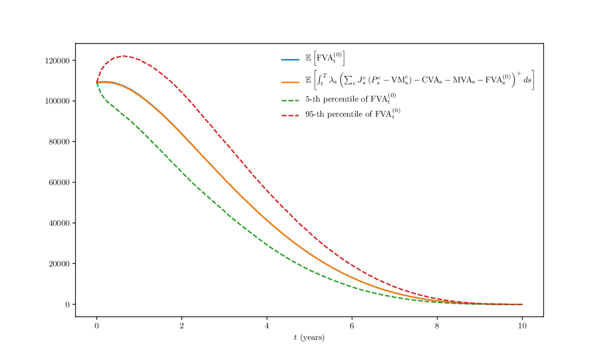
Figure 10 (left) is a sanity check that the profiles of the successives iterates of the shareholder trading loss process in Algorithm 1 converge rapidly with . Figure 10 (right) shows the loss process , displayed as its mean and mean 2 stdev profiles. Consistent with its martingale property, the loss process appears numerically centered around zero. The latter holds, at least, beyond years. For earlier times, the regression errors, accumulated backward across pricing times since the final maturity of the portfolio, induce a non negligible bias (the corresponding confidence intervals no longer contains 0). This is the reason why we use a coarser pricing time step than simulation time step in Algorithm 1.


5.2 Portfolio-wide XVA Profiles
For the financial case study that follows, we consider
- •
swap rates uniformly distributed on (hence swaps already in-the-money or out-of-the-money at time 0),
- •
number of six-monthly coupon resets uniform on (final maturity of the portfolio years),
- •
portfolio direction: either “asset heavy” bank mostly in the receivables in the future, or “liability-heavy” bank mostly in the payables in the future (respectively corresponding, with our data, to a bank likely to pay fixed in the swaps, or likely to receive fixed).
The figures that follow only display profiles, i.e. term structures, that is, expectations as a function of time of the corresponding processes. But all these processes are computed pathwise, based on the deep learning regression and quantile regression methodology of Section 4.4, allowing for all XVA inter-dependencies. Of course, XVA profiles (or pathwise XVAs if wished) are much more informative for traders than the spot XVA values (or time 0 confidence intervals) returned by most XVA systems.
Assuming 10 counterparties, Figure 11 shows the GPU generated profiles of
| (48) |
in the case of the asset-heavy portfolio and of the liability-heavy portfolio.


Figure 12 shows the porftolio-wide XVA profiles of the asset-heavy (top) vs. liability–heavy (bottom) portfolio and of the no CSA (left) vs. CSA portfolio (right). Obviously, asset–heavy or no CSA means more CVA. The correponding curves also emphasize the transfer from counterparty credit into liquidity funding risk prompted by extensive collateralisation. Yet FVA/MVA risk is ignored in current derivatives capital regulation.


Figure 13 shows that (top left) capital at risk as funding (cf. Section 3.4) has a material impact on the already (reserve capital as funding) reduced FVA, (top right) treating KVA as a risk margin (cf. (26)) gives a huge discounting impact, (bottom left) deep learning detects material initial margin convexity in the asset-heavy CSA portfolio, and (bottom right) deep learning detects material economic capital convexity in the asset-heavy no CSA portfolio.


The above findings demonstrate the necessity of pathwise capital and margin calculations for accurate FVA, MVA, and KVA calculations.
5.3 Trade Incremental XVA Profiles
Next, we consider, on top of the previous portfolios, an incremental trade given as a par 30 year (receive fix or pay fix) swap with 100K notional. Figure 14 shows the trade incremental XVA profiles produced by our deep learning approach. Note that, for obtaining such smooth incremental profiles, it has been key to use common random numbers, as much as possible, between the original portfolio XVA computations and the ones regarding the portfolio expanded with the new trade.


5.4 Trade and Hedge Incremental XVA Profiles
Our model assumes the market risk of trades to be fully hedged (see the paragraph following Remark 2.2 and the proofs of Lemma 3.2 and Proposition 4.1). In the previous subsection, the new swap was implicitly meant to be hedged, in terms of market risk, by the clean desks, through an accordingly modified hedging loss process (see Section 2.1). Here we consider an alternative situation where the market risk of the new swap is back-to-back hedged via a financial, hedge counterparty. Specifically, we deal with
- •
10 counterparties: 8 no CSA clients and 2 bilateral VM/IM CSA hedge counterparties,
- •
portfolios of 5K randomly generated swap trades as before, plus 5K corresponding hedge trades,
- •
an incremental trade given as a par 30 year swap with 100K notional, along with the corresponding hedge trade.
In particular, (cf. (48)), in both portfolios excluding or including the new swap. In case a client or hedge counterparty defaults, the corresponding market hedge is assumed to be rewired through the clean desks via an accordingly modified hedging loss process .
The 8 no CSA counterparties are primarily asset or liability heavy. One bilateral CSA hedge counterparty is asset-heavy and one liability-heavy. Figure 15 provides the trade incremental XVA profiles of the bilateral hedge alternatives in combination with those for the initial counterparty trade. The main XVA impact of the hedge is then a corresponding incremental MVA term, which can contribute to make the global FTP related to the trade+hedge package more or less positive or negative, depending on the data (cf. the four panels in Figure 15), as can only be inferred by a refined XVA computation.


Remark 5.1
In the above, we do not include the XVA costs/benefits of the bilateral hedge counterparty itself. Given Remark 2.4, in different circumstances it may be possible to attribute them to client trades of the original or hedge bank. Space is lacking for a fuller discussion of economics of XVA trading in different setups. In particular, many hedge trades now face central instead of bilateral counterparties. This occurs at additional XVA costs for the client of the initial swap that can be computed the way explained in ?).
5.5 Scalability
Our deep learning XVA implementation uses CNTK, the Microsoft Cognitive Toolkit. CNTK is written in core C++/CUDA (with wrappers for Python, C#, and Java). This is convenient for XVA applications, which are usually developed in C++: CNTK automatic differentiation in C++/CUDA enables C++ in-process training. This allows embedding the deep learning task within XVA processing.
Table 5 sets out computation times, including additional results obtained by doubling the numbers of counterparties and risk factors (to 20 counterparties and 80 risk factors).
| 10 CP 40 risk factors | 20 CP 80 risk factors | |||
| No CSA | IM CSA | No CSA | IM CSA | |
| Initial risk factor & trade pricing simulation Cuda | 352 | 352 | 426 | 426 |
| Counterparty and bank level learning calculations | 4,529 | 13,466 | 19,154 | 59,342 |
| Total initial batch | 4,881 | 13,818 | 19,580 | 59,768 |
| Re-simulate 1 counterparty trade pricing Cuda | 40 | 40 | 51 | 51 |
| Counterparty and bank level learning calculations | 2,785 | 2,736 | 7,694 | 6,628 |
| Total incremental trade | 2,825 | 2,776 | 7,745 | 6,679 |
All these results were based on 50K simulation paths, 32 time steps per year for risk factor simulation, and 16 time steps per year for all XVA calculations and deep learning. They were computed on a Lenovo P52 laptop with NVidia Quadro P3200 GPU @ 5.5 Teraflops peak FP32 performance, and 14 streaming multiprocessors.
The computations for 20 counterparties took more than twice as long as those for 10 counterparties. However, our deep learning calculations achieved around 80 to 90% Cuda occupancy for 10 counterparties and at times fell to half that level for 20 counterparties. Scaling to realistically high dimensions should be achievable, but acceptable trade incremental pricing performance in production would require server-grade GPU hardware, performance tuning for high GPU utilisation, and, possibly, caching computations.
Appendix A Continuous-Time XVA Equations
We recall from ?) the continuous-time XVA equations for bilateral trade portfolios when capital at risk is deemed fungible with variation margin, also adding here initial margin and MVA as in the refined static setup of Section 3.4.
We write for the Dirac measure at a random time .
A.1 Cash Flows
We suppose that the derivative portfolio of the bank is partitioned into bilateral netting sets of contracts which are jointly collateralized and liquidated upon bank or counterparties (whether these are clients or market hedge counterparties) default. Given a netting set of the bank portfolio, we denote by:
- •
and , the corresponding contractually promised cash flows and clean value processes;
- •
, , and , the corresponding default times, survival indicators, and recovery rates, whereas , , and are the analogous data regarding the bank itself, with bank credit spread process taken as a proxy of its risky funding spread process99 9 See ?, Section 5) for the discussion of cheaper funding schemes for initial margin.;
- •
and , where is a positive margin period of risk, in the sense that the liquidation of the netting set happens at time ;
- •
the variation margin (re-hypothecable collateral) exchanged between the bank and counterparty , counted positively when received by the bank;
- •
and , the related initial margin (segregated collateral) posted and received by the bank;
- •
and , the reserve capital and capital at risk of the bank.
The contractually promised cash flows are supposed to be hedged out by the bank but one conservatively assumes no XVA hedge, so that the bank is left with the following trading cash flows and (cf. (38) and see ?, Lemmas 5.1 and 5.2) for detailed derivations of analogous equations in a slightly simplified setup):
- •
The (counterparty) credit cash flows
(49) - •
The (risky) funding cash flows
(50) where the and terms account for the fungibility of reserve capital and capital at risk with variation margin.
A.2 Valuation
Here (as in our numerics) we distinguish between a (strict) FVA, in the strict sense of the cost of raising variation margin, and an MVA for the cost of raising initial margin (see Remark 2.1). The (other than K)VA equations are then
| (51) |
the so-called “contra-assets valuation” sourced from the clients and deposited in the reserve capital account of the bank, where, for ,
| (52) |
The corresponding trading loss and profit process of the bank is such that
| (53) |
so that is a martingale, hence (by Lemma 4.1) is a martingale.
Definition A.1
is the time- conditional 97.5% expected shortfall of () under .
Given a positive target hurdle rate :
Definition A.2
We set
| (54) |
for a process such that, for ,
| (55) |
Hence, for ,
| (56) |
The next-to-last identity is the continuous-time analog of the risk margin formula under the Swiss solvency test cost of capital methodology: see ?, Section 6, middle of page 86 and top of page 88).
A.3 The XVA Equations are Well-Posed
In view of (51), the second line in (52) is in fact an equation. Likewise, the second line in (56) is a equation. Moreover, as capital at risk is fungible with variation margin (cf. Section 3.4), i.e. in consideration of the term in (52)-(53), where , we actually deal with an system, and even, as EC depends on (cf. Definition A.1), with a forward backward system for the forward loss process and the backward pair .
However, as in the refined static setup of Section 3.4, the coupling between and can be disentangled by the following Picard iteration:
- •
- •
For writing explicitly to emphasize the dependence of on , let and, for ,
(58)
Theorem 4.1 in ?)
Assuming square integrable data, the XVA equations are well-posed within square integrable solution (including when one accounts for the fact that capital at risk can be used for funding variation margin). Moreover, the
above Picard iteration
converges to the unique square integrable solution of the XVA equations.
A.4 Collateralization Schemes
We denote by the cumulative contractual cash flows with the counterparty accumulated over a past period of length . In our case study, we consider both “no CSA” netting sets , with , and “(VM/IM) CSA” netting sets , with and, for ,
| (59) |
for some PIM and RIM quantile levels and (and ).
The following result can be derived by similar computations as the ones in ?, Section A).
Proposition A.1
In a common shock default model of the counterparties and the bank itself (see the beginning of Section 5), with pre-default intensity processes of the counterparties and of the bank, then , where, for
| (60) | |||
| (61) | |||
where () in (61) is computed at the confidence level. Assuming its posted initial margin borrowed unsecured by the bank, then , where, for
| (62) |
References
- Abbas-Turki, Diallo, and Crépey (2018 Abbas-Turki, L., B. Diallo, and S. Crépey (2018). XVA principles, nested Monte Carlo strategies, and GPU optimizations. International Journal of Theoretical and Applied Finance 21, 1850030.
- Albanese, Armenti, and Crépey (2020 Albanese, C., Y. Armenti, and S. Crépey (2020). XVA Metrics for CCP optimisation. Statistics & Risk Modeling 37(1-2), 25–53.
- Albanese, Caenazzo, and Crépey (2017 Albanese, C., S. Caenazzo, and S. Crépey (2017). Credit, funding, margin, and capital valuation adjustments for bilateral portfolios. Probability, Uncertainty and Quantitative Risk 2(7), 26 pages.
- Albanese and Crépey (2020 Albanese, C. and S. Crépey (2020). The cost-of-capital XVA approach in continuous time. Working paper available on https://math.maths.univ-evry.fr/crepey.
- Andersen, Duffie, and Song (2019 Andersen, L., D. Duffie, and Y. Song (2019). Funding value adjustments. Journal of Finance 74(1), 145–192.
- Artzner, Eisele, and Schmidt (2020 Artzner, P., K.-T. Eisele, and T. Schmidt (2020). No arbitrage in insurance and the QP-rule. Working paper available as arXiv:2005.11022.
- Barrera, Crépey, Diallo, Fort, Gobet, and Stazhynski (2019 Barrera, D., S. Crépey, B. Diallo, G. Fort, E. Gobet, and U. Stazhynski (2019). Stochastic approximation schemes for economic capital and risk margin computations. ESAIM: Proceedings and Surveys 65, 182–218.
- Beck, Becker, Cheridito, Jentzen, and Neufeld (2019 Beck, C., S. Becker, P. Cheridito, A. Jentzen, and A. Neufeld (2019). Deep splitting method for parabolic PDEs. arXiv:1907.03452.
- Bichuch, Capponi, and Sturm (2018 Bichuch, M., A. Capponi, and S. Sturm (2018). Arbitrage-free XVA. Mathematical Finance 28(2), 582–620.
- Bielecki and Rutkowski (2002 Bielecki, T. and M. Rutkowski (2002). Credit Risk: Modeling, Valuation and Hedging. Springer Finance, Berlin.
- Bielecki and Rutkowski (2015 Bielecki, T. R. and M. Rutkowski (2015). Valuation and hedging of contracts with funding costs and collateralization. SIAM Journal on Financial Mathematics 6, 594–655.
- Brigo and Capponi (2010 Brigo, D. and A. Capponi (2010). Bilateral counterparty risk with application to CDSs. Risk Magazine, March 85–90. Preprint version available at https://arxiv.org/abs/0812.3705.
- Brigo and Pallavicini (2014 Brigo, D. and A. Pallavicini (2014). Nonlinear consistent valuation of CCP cleared or CSA bilateral trades with initial margins under credit, funding and wrong-way risks. Journal of Financial Engineering 1, 1–60.
- Burgard and Kjaer (2011 Burgard, C. and M. Kjaer (2011). In the balance. Risk Magazine, October 72–75.
- Burgard and Kjaer (2013 Burgard, C. and M. Kjaer (2013). Funding costs, funding strategies. Risk Magazine, December 82–87. Preprint version available at https://ssrn.com/abstract=2027195.
- Burgard and Kjaer (2017 Burgard, C. and M. Kjaer (2017). Derivatives funding, netting and accounting. Risk Magazine, March 100–104. Preprint version available at https://ssrn.com/abstract=2534011.
- Castagna (2014 Castagna, A. (2014). Towards a theory of internal valuation and transfer pricing of products in a bank: Funding, credit risk and economic capital. Available at http://ssrn.com/abstract=2392772.
- Collin-Dufresne, Goldstein, and Hugonnier (2004 Collin-Dufresne, P., R. Goldstein, and J. Hugonnier (2004). A general formula for valuing defaultable securities. Econometrica 72(5), 1377–1407.
- Committee of European Insurance and Occupational Pensions Supervisors (2010 Committee of European Insurance and Occupational Pensions Supervisors (2010). QIS5 technical specifications. https://eiopa.europa.eu/Publications/QIS/QIS5-technical_specifications_20100706.pdf.
- Crépey (2015 Crépey, S. (2015). Bilateral counterparty risk under funding constraints. Part I: Pricing, followed by Part II: CVA. Mathematical Finance 25(1), 1–22 and 23–50. First published online on 12 December 2012.
- Crépey, Bielecki, and Brigo (2014 Crépey, S., T. R. Bielecki, and D. Brigo (2014). Counterparty Risk and Funding: A Tale of Two Puzzles. Chapman & Hall/CRC Financial Mathematics Series.
- Crépey, Sabbagh, and Song (2020 Crépey, S., W. Sabbagh, and S. Song (2020). When capital is a funding source: The anticipated backward stochastic differential equations of X-Value Adjustments. SIAM Journal on Financial Mathematics 11(1), 99–130.
- Crépey and Song (2016 Crépey, S. and S. Song (2016). Counterparty risk and funding: Immersion and beyond. Finance and Stochastics 20(4), 901–930.
- Crépey and Song (2017 Crépey, S. and S. Song (2017). Invariance times. The Annals of Probability 45(6B), 4632–4674.
- Dimitriadis and Bayer (2019 Dimitriadis, T. and S. Bayer (2019). A joint quantile and expected shortfall regression framework. Electronic Journal of Statistics 13(1), 1823–1871.
- Duffie and Huang (1996 Duffie, D. and M. Huang (1996). Swap rates and credit quality. Journal of Finance 51, 921–950.
- Duffie and Sharer (1986 Duffie, D. and W. Sharer (1986). Equilibrium and the role of the firm in incomplete market. Stanford University, Working Paper No. 915, available at https://www.gsb.stanford.edu/faculty-research/working-papers/equilibrium-role-firm-incomplete-markets.
- Dybvig (1992 Dybvig, P. (1992). Hedging non-traded wealth: when is there separation of hedging and investment. In S. Hodges (Ed.), Options: recent advances in theory and practice, Volume 2, pp. 13–24. Manchester University Press.
- Elouerkhaoui (2007 Elouerkhaoui, Y. (2007). Pricing and hedging in a dynamic credit model. International Journal of Theoretical and Applied Finance 10(4), 703–731.
- Elouerkhaoui (2017 Elouerkhaoui, Y. (2017). Credit Correlation: Theory and Practice. Palgrave Macmillan.
- Fissler and Ziegel (2016 Fissler, T. and J. Ziegel (2016). Higher order elicitability and Osband’s principle. The Annals of Statistics 44(4), 1680–1707.
- Fissler, Ziegel, and Gneiting (2016 Fissler, T., J. Ziegel, and T. Gneiting (2016). Expected Shortfall is jointly elicitable with Value at Risk—Implications for backtesting. Risk Magazine, January.
- Föllmer and Schied (2016 Föllmer, H. and A. Schied (2016). Stochastic Finance: An Introduction in Discrete Time (4th ed.). De Gruyter Graduate.
- Goodfellow, Bengio, and Courville (2016 Goodfellow, I., Y. Bengio, and A. Courville (2016). Deep Learning. MIT Press.
- Gottardi (1995 Gottardi, P. (1995). An analysis of the conditions for the validity of Modigliani-Miller Theorem with incomplete markets. Economic Theory 5, 191–207.
- Green, Kenyon, and Dennis (2014 Green, A., C. Kenyon, and C. Dennis (2014). KVA: capital valuation adjustment by replication. Risk Magazine, December 82–87. Preprint version “KVA: capital valuation adjustment” available at ssrn.2400324.
- Hoeting, Madigan, Raftery, and Volinsky (1999 Hoeting, J. A., D. Madigan, A. E. Raftery, and C. T. Volinsky (1999). Bayesian model averaging: A tutorial. Statistical Science 14(4), 382–417.
- Hull and White (2012 Hull, J. and A. White (2012). The FVA debate, followed by The FVA debate continued. Risk Magazine, July 83–85 and October 52.
- Huré, Pham, and Warin (2020 Huré, C., H. Pham, and C. Warin (2020). Some machine learning schemes for high-dimensional nonlinear PDEs. Mathematics of Computation 89(324), 1547–1580.
- International Financial Reporting Standards (2013 International Financial Reporting Standards (2013). IFRS 4 insurance contracts exposure draft.
- Kjaer (2019 Kjaer, M. (2019). In the balance redux. Risk Magazine (November).
- Longstaff and Schwartz (2001 Longstaff, F. A. and E. S. Schwartz (2001). Valuing American options by simulation: A simple least-squares approach. The Review of Financial Studies 14(1), 113–147.
- Merton (1974 Merton, R. (1974). On the pricing of corporate debt: the risk structure of interest rates. The Journal of Finance 29, 449–470.
- Modigliani and Miller (1958 Modigliani, F. and M. Miller (1958). The cost of capital, corporation finance and the theory of investment. Economic Review 48, 261–297.
- Myers (1977 Myers, S. (1977). Determinants of corporate borrowing. Journal of Financial Economics 5, 147–175.
- Piterbarg (2010 Piterbarg, V. (2010). Funding beyond discounting: collateral agreements and derivatives pricing. Risk Magazine, August 57–63.
- Schönbucher (2004 Schönbucher, P. (2004). A measure of survival. Risk Magazine 17(8), 79–85.
- Swiss Federal Office of Private Insurance (2006
Swiss Federal Office of Private Insurance (2006).
Technical document on the Swiss solvency test.
https://www.finma.ch/FinmaArchiv/bpv/download/e/
SST_techDok_061002_E_wo_Li_20070118.pdf.