Muonization of supernova matter
Abstract
The present article investigates the impact of muons on core-collapse supernovae,
with particular focus on the early muon neutrino emission. While the presence of
muons is well understood in the context of neutron stars, until the recent study
by Bollig et al. [Phys. Rev. Lett. 119, 242702 (2017)] the role of muons
in core-collapse supernovae had been neglected—electrons and neutrinos were
the only leptons considered. In their study, Bollig et al. disentangled the muon
and tau neutrinos and antineutrinos and included a variety of muonic weak
reactions, all of which the present paper follows closely. Only then does it
becomes possible to quantify the appearance of muons shortly before stellar
core bounce and how the post-bounce prompt neutrino emission is modified.
DOI: 10.1103/PhysRevD.102.123001
I Introduction
A core-collapse supernova (SN) determines the final fate of all stars more massive than about 8 M⊙. The associated stellar core collapse is triggered due to deleptonization by nuclear electron capture in the core and the subsequent escape of the electron neutrinos produced, lowering the degenerate electron density responsible for supporting the core against gravity, and to the photo-disintegration of heavy nuclei in the core, sapping thermal, pressure-producing energy as well. The collapse halts when the central density exceeds normal nuclear density. The repulsive short-range nuclear force reverses the collapse, and the stellar core rebounds. An expanding shock wave forms, which stalls when crossing the neutrinospheres, the surfaces of last scattering for the neutrinos produced and trapped during core collapse. A large number of electron captures on the newly liberated protons from the dissociation of nuclei by the shock releases the deleptonization burst after the shock passes the neutrinospheres. This happens on a timescale of about 5–20 ms after core bounce Janka et al. 2007; Janka 2012. The central compact object comprising a cold, un-shocked core and a hot, shocked mantle is the proto-neutron star (PNS). The so-called SN problem poses the question: How is the stalled bounce shock revived? Several scenarios have been proposed: the neutrino heating Bethe and Wilson 1985, magneto-rotational LeBlanc and Wilson 1970, and acoustic Burrows et al. 2006 mechanisms, as well as a mechanism associated with a high-density phase transition in the core Sagert et al. 2009; Fischer et al. 2018; Fischer et al. 2020a. Studies of the multi-physics, multi-scale core-collapse SN phenomenology require large-scale computer models, which are based on neutrino radiation- hydrodynamics. For a recent review about the various scales and conditions of relevance, as well as the SN equation of state (EOS), cf. Ref. Müller 2016; Fischer et al. 2017.
During a core-collapse SN, the neutrinos propagate through regions that are diffusive, semitransparent, and transparent (where the neutrinos simply stream freely). Thus, the neutrinos are not fluid-like everywhere, and a full Boltzmann kinetic treatment of neutrino transport is ultimately necessary. This has been achieved in the context of general relativistic models in spherical symmetry Yamada et al. 1999; Liebendörfer et al. 2001 and in axisymmetry Chan and Müller 2020, as well as non-relativistic and relativistic axisymmetric models with Newtonian gravity Ott et al. 2008; Nagakura et al. 2018. While pioneering and already advancing with respect to treating separately and , all of these studies suffer from a draw back: they assume equal distributions of - and -neutrinos and antineutrinos.
This simplification can only be justified in the absence of muons. However, it is well known for cold neutron stars, where due to the condition of -equilibrium muons and electrons have equal chemical potentials (). Hence, when MeV, the muon fraction can be as large as (depending on the nuclear EOS) above a rest-mass density of about half the saturation density ( g cm-3). The presence of muons has important consequences for the long-term cooling of neutron stars; e.g., it modifies the direct-Urca threshold Glendenning 1996. Muons have to be produced at some point during the evolution of the PNS from a hot lepton rich object to the cold -equilibrium object discussed above. However, this aspect has only been recently studied in Ref. Bollig et al. 2017, including the possibility of muons decaying to axions Bollig et al. 2020. Muons can be produced in non-negligible abundances during a core-collapse SN. The present article extends this study to consider the muonization of SN matter shortly before core bounce and discusses the impact of the presence of muons on the neutrino emission up to shortly after core bounce. Therefore, the Boltzmann neutrino transport scheme is extended to treat - and -neutrinos and antineutrinos separately, include an extended set of weak processes with muons in the collision integral on the right-hand side of the Boltzmann equation, and add the muon abundance as an additional independent degree of freedom in the radiation-hydrodynamics scheme.
The present article is organized as follows. In Sec. II, the SN model is briefly reviewed, with special emphasis placed on the updates to the neutrino transport scheme. Sec. III discusses our SN simulation results in close proximity of stellar core bounce, with a focus on the muonization of SN matter and on the enhanced muon-neutrino luminosity. In Sec. IV, we consider the possibility for convection to occur due to the presence of what will now be an additional lepton number gradient. The manuscript closes with a summary in Sec. V.
II Core-collapse supernova model
The core-collapse SN model employed in this study, AGILE-BOLTZTRAN, is based on general relativistic neutrino radiation hydrodynamics in spherical symmetry Mezzacappa and Bruenn 1993a; Mezzacappa and Bruenn 1993b; Mezzacappa and Bruenn 1993, in comoving coordinates Liebendörfer et al. 2001; Liebendörfer et al. 2004 with a Lagrangian mesh featuring an adaptive mesh refinement method Liebendörfer et al. 2002. In the present study 207 radial mass zones are used. A recent global-comparison core-collapse SN study in spherical symmetry, including AGILE-BOLTZTRAN, can be found in Ref. O’Connor et al. 2018.
II.1 Equation of state
AGILE-BOLTZTRAN has a flexible EOS module treating separately the nuclear part Hempel et al. 2012 and the electron/positron/photon/Coulomb EOS; the latter is collectively denoted as EPEOS Timmes and Arnett 1999. In addition to the temperature, , and restmass density, , the EOS depends also on the nuclear composition with mass fractions , atomic mass and charge . The latter determines the charge fraction of the nuclei, which balances the combined charge fractions of electrons, and muons, . Here, the nuclear EOS of Ref. Hempel and Schaffner-Bielich 2010 is employed. It is based on the modified nuclear statistical equilibrium approach for several 1000 nuclear species and the density- dependent relativistic mean-field model DD2 Typel et al. 2010 for the unbound nucleons.
In the present study, a muon EOS is implemented in AGILE-BOLTZTRAN. Therefore, the following muon EOS quantities are tabulated: particle density , internal energy density , pressure and entropy per particle , as a function of the muon chemical potential ranging MeV for a large range of temperatures from MeV. The Fermi integrals are performed numerically with a 64-point Gauss-quadrature. This ensures thermodynamic consistency. Since muons are massive leptons, their restmass cannot be neglected, and the relativistic dispersion relation must be employed, , unlike electrons/positrons, which are ultrarelativistic (). In the SN simulations, where the muon abundance becomes the degree of freedom for the muon EOS, in addition to temperature and restmass density, a linear interpolation is used to find the corresponding muonic thermodynamic state, , , and , respectively. These quantities, except , are then added to the corresponding quantities for baryons (B) and EPEOS, in order to obtain the total quantities,
| (1) | |||||
| (2) | |||||
| (3) | |||||
Note that the baryon EOS contributions depend on the hadronic charge fraction via the charge-neutrality conditions, , where electron and muon abundances are associated with their corresponding net particle densities, such that and .
II.2 Boltzmann neutrino transport
The neutrino transport scheme has to be extended in order to be able to treat individually the distributions for all 3 flavors, and their respected antineutrinos . BOLTZTRAN employs an operator-split method to solve the evolution equations for the neutrino distribution functions, as described in detail in Ref. Liebendörfer et al. 2004 (steps 1.–3. outlined in sec. 3.5). Each implicitly finite differencing update of the transport equation includes the update of the evolution of the temperature and the electron/muon fraction due to weak interactions, as well as corrections due to advection. A Newton-Raphson scheme is implemented to solve the implicitly finite differencing nonlinear equations. Beginning with (), this procedure is repeated for () and (). As was outlined already in Ref. Liebendörfer et al. 2004, this cycling ensures that the neutrino distribution functions are in accurate equilibrium with matter after obtaining the solution of the transport equation and updating temperature and electron fraction accordingly. However, it introduces a mismatch of the radial grid of the new hydrodynamics variables due to the corrections of the advection equation. Note further that for the weak processes, , where initial the final state neutrino distributions belong to different species Buras et al. 2006, in the collision integral of the Boltzmann transport equation we assume equilibrium distributions as was outlined in Ref. Fischer et al. 2009. This approach is inadequate for the purely leptonic weak processes involving muons, which will be introduced below, where initial the final state neutrino distributions also belong to different species. Here we implement for the final states the actual neutrino distributions from the previous cycling, which introduces a slight mismatch that we monitor carefully with an increased accuracy required for the neutrino transport convergence.
Note further that BOLTZTRAN employs the transport equation in conservative form; i.e. with the specific neutrino distribution function, Mezzacappa and Bruenn 1993a; Mezzacappa and Bruenn 1993b. All neutrino species are discretized in terms of 6 momentum angles bins 11 1 is used here and not as in the standard literature, not to confuse with the muons – the angle between the radial motion and the momentum vector – and 36 neutrino energy bins, MeV following the setup of S. Bruenn Bruenn 1985. Appendix A compares two SN simulations, both without muonic weak reactions, comparing the traditional Boltzmann transport scheme for 4 neutrino species (, , , ) and the full 6 neutrino species transport (, , , , , ). While the extension to 6-species Boltzmann neutrino transport is straight forward, the inclusion of weak interactions and the associated extensions of the collision-integral involving weak reactions with (anti)muons will be discussed in the next sections. Further details are given in Appendix B.
II.3 Muonic weak processes
In the following subsections all new weak reactions involving (anti)muons, which are being implemented in AGILE-BOLTZTRAN, will be discussed. Table 1 lists all processes considered here. Further details, about the reaction rates are provided in Appendix B, see also Ref. Guo et al. 2020, and details about their implementation in AGILE-BOLTZTRAN are provided in Appendix B of the present paper.
II.3.1 Charged-current absorption and emission
For the emissivity and absorptivity for the muonic charged-current (CC) reactions (1a) and (1b) in Table 1, the fully inelastic and relativistic rates are employed. These rates were developed in Ref. Guo et al. 2020, Section III A, which is based on the same treatment as for the electronic CC rates Fischer et al. 2020b. Ref. Oertel et al. 2020 consider correlations at the level of the random-phase approximation but neglect contributions from weak-magnetism which we take self-consistently into account. Furthermore, the rate expressions of Ref. Guo et al. 2020 consider pseudo-scalar interaction contributions.
| Label | Weak process | Abbreviation |
|---|---|---|
| (1a) | CC | |
| (1b) | CC | |
| (2a) | NMS | |
| (2b) | NMS | |
| (3a) | LFE | |
| (3b) | LFE | |
| (4a) | LFC | |
| (4b) | LFC |

| 22 2 are the neutron/proton single-particle potentials, which are given by the DD2 EOS | |||||||||||||||||||||
|---|---|---|---|---|---|---|---|---|---|---|---|---|---|---|---|---|---|---|---|---|---|
| MeV | g cm | MeV | MeV | MeV | |||||||||||||||||
| (a) | 10 | 0.2 | 108.1 | 51.7 | 13.9 | ||||||||||||||||
| (b) | 25 | 0.15 | 0.05 | 147.4 | 132.8 | 31.5 |
Equations (27)–(33) in Ref. Guo et al. 2020, as well as their Appendix (B), summarize the entire algebraic expressions. Since the transition amplitudes – the spin averaged and squared matrix elements – are identical for electronic and muonic charged-current reactions, the only difference is the remaining phase space. Hence, the only replacements for the muonic charged-current rates are the different muon restmass and the muon Fermi distribution function with the corresponding muon chemical potential. These fully inelastic charged-current absorption rates are shown in Fig. 1 (solid lines) for (left panel) and (right panel) at two selected conditions, in comparison with the CC rates in the elastic approximation (see Appendix B.1). For the elastic rates we include the approximate treatment of inelasticity and weak magnetism corrections Horowitz 2002 via ()-energy dependent multiplicative factors.
| Scattering process | 33 3 | ||
|---|---|---|---|
For and energies below the values of and , respectively, there can be no contribution to the opacity within the elastic treatment (details about the elastic rate expression are given in Appendix B.1), as illustrated in Fig. 1 (dashed lines) at two selected conditions (a) and (b), which are listed in Table 2. This strong opacity drop is modified when taking into account inelastic contributions within the full kinematics approach, as illustrated in Fig. 1 (solid lines). Since these muonic CC processes are expected to be responsible for the muonization of SN matter, from Fig. 1 it becomes evident this channel requires of high energy in order to produce final state muons in non-negligible amounts.


II.3.2 Neutrino–muon scattering
For neutrino–muon scattering (NMS), reactions (2a) and (2b) in Table 1, the approach for neutrino–electron scattering (NES) is employed here following the detailed derivation provided in Refs. Tubbs and Schramm 1975; Schinder and Shapiro 1982; Bruenn 1985; Mezzacappa and Bruenn 1993, which is equivalent to the recent derivation in Ref. Guo et al. 2020, Section II A and Appendix A. Mapping the algebraic expressions of NES to NMS is straightforward due to the similarity of the transition amplitudes and hence of the scattering kernels between NES and NMS. It requires the replacement of electron restmass and chemical potential with those of the muons. However, the vector and axial-vector coupling constants are different for NES and NSM, which are listed in Table 3. Details about the scattering amplitudes and in/out scattering kernels for NMS, , are provided in Appendix B.2, together with their implementation in the collision integral of AGILE-BOLTZTRAN.


In Fig. 2 we compare the opacity for neutrino– scattering (dashed lines) and neutrino– scattering (solid lines) at two selected conditions (a) and (b), for which the thermodynamic conditions are listed in Table 2. In order to obtain the neutrino-scattering opacity, the following integration is performed of the out-scattering kernel, , over the final-state neutrino phase space,
| (4) | |||||
i.e. assuming a free-final state neutrino phase space (more details can be found in Ref. Fischer et al. 2012). The scattering kernel depends on the in-coming and the out-going neutrino energies, and , as well as the in-coming and out-going relative angles, and (see Appendix B).
Note that neutrino trapping and thermalization of and neutrinos occurs roughly at the conditions between (a) and (b) of Table 2. Hence, neutrino–muon scattering may be an important source for the thermalization and trapping of heavy lepton-flavor neutrinos. Furthermore, from the comparison in Fig. 2 it becomes evident that at high densities, muon-neutrino scattering on muons dominates over scattering on electrons. This is mostly attributed to the high electron degeneracy due to which the final-state electron phase space is occupied. Note also that, at such conditions (b), neutrinos are trapped.


Since the opacity shown in Fig. 2 does not reveal insights into the inelasticity of the processes, in Fig. 3 we show in addition the angular-averaged outgoing scattering kernels defined as follows,
| (5) | |||||
as a function of the outgoing neutrino energy, , for three different incoming neutrino energies, , evaluated at the two conditions (a) and (b) listed in Table 2 shown in Figs. 3 and 3, respectively. Low incoming neutrino energies (left panels in Fig. 3) both NMs (solid lines) and NES (dashed-dotted lines) are dominated by down-scattering, due to the electrons being degenerate and, since muons are never degenerate under SN conditions, the high muon restmass. With increasing (middle and right panels in Fig. 3) the restmass contribution becomes less important, and the differences between NMS and NES are due to the different degeneracy.
In addition, Figure 4 shows the dependence of the scattering kernel on the total scattering angle, for the conditions (a) in Table 2 (left panels) and the conditions (b) in Table 2 (right panels), assuming thermal energies for the initial neutrinos; i.e., and for different out-going neutrino energies Therefor, the top panel in Fig. 4 assumes out-scattering energies which are equal to the peak of the scattering kernel; i.e. MeV (NMS) and MeV (NES) for MeV corresponding to conditions (a) in Table 2 ( MeV), from where it becomes evident that NES is mainly forward peaked at an angle of about 30 degrees while NMS is more isotropic. Note that the scale in Figs. ref4(a) and 4(b) are logarithmic. At the conditions illustrated in Fig. 4(c), which correspond to out-scattering energies being equal to the peak of the scattering kernels plus the half-width (see the left panel in Fig. 3), both NMS and NES are strongly forward peaked. This situation is reversed in Fig. 4(e) where the out-scattering energy is equal to the peak of the scattering kernel minus the half-width, when both NMS and NES are back-scattering dominated with NMS being more isotropic. This situation remains the same at higher density and MeV ( MeV) orresponding to the conditions (b) in Table 2, illustrated in Figs. 4(b) 4(d) and 4(f) (for the scattering kernel, see the middle panel in Fig. 3).
II.3.3 Purely leptonic reactions – (i) lepton flavor exchange
A new class of weak processes, known as lepton flavor exchange (LFE) reactions Bollig et al. 2017, is added to AGILE-BOLTZTRAN, reactions (3a) and (3b) of Table 1. The close analogy of the scattering amplitudes of NMS and LFE, enables the direct comparison between these two processes, which simplifies the calculation of the in- and out-scattering kernels, provided in detail in Appendix B.3.1 where the nomenclature of Ref. Mezzacappa and Bruenn 1993 is followed closely. It is equivalent to the recent derivation in Ref. Guo et al. 2020, Section II A and Appendix A.
The main difference between NMS and LFE is the appearance of a new energy scale since initial- and final-state leptons are different; one has to take the restmass energy difference between muon and electron into account. This gives rise to additional terms in the scattering amplitudes (they are provided in Appendix B.3.1), which can be large.
Figure 5 compares the set of the LFE processes (3a) and (3b) in Table 1, for each channel individually at the two selected conditions (a) and (b) corresponding to Table 2. For the calculation of the opacity the same approach is implemented here as for neutrino–muon scattering Eq. (4); i.e., assuming a free final-state neutrino. These rates are in agreement with those obtained in Ref. Guo et al. 2020 with a detailed comparison of the LFE rates and the muonic CC rates.


II.3.4 Purely leptonic reactions – (ii) lepton flavor conversion
There is a second class of purely leptonic processes involving (anti)muons, known as lepton flavor conversion reactions (LFC) Bollig et al. 2017, reactions (4a) and (4b) in Table 1. The derivation of the in- and out-scattering kernels is given in Appendix B.3.2, again in close analogy to Ref. Guo et al. 2020. Figure 5 compares the rates for the LFC processes, at the same two selected conditions (a) and (b) of Table 2, as before. This comparison is in agreement with the analysis of Ref. Guo et al. 2020.
All these weak reaction rates involving muons, i.e. muonic CC rates and NMS as well as the LFE and LFC processes, are implemented in AGILE-BOLTZTRAN within the 6-species setup, in order to simulate and study the impact of the muonization of SN matter. In the following, these results will be discussed as the reference case and compared to the simulations where all muonic weak rates are set to zero. Note that we omit here the (inverse) muon decay.
III Core-collapse SN simulations
The core-collapse SN simulations discussed in the following are launched from the 18 M⊙ progenitor from the stellar evolution series of Ref. Woosley et al. 2002. Besides the muonic weak processes introduced in Sec. II above, the standard set of non-muonic weak reactions employed here is given in Table (1) of Ref. Fischer et al. 2020b. A comparison of these non-muonic weak rates in the ‘minimal’ setup of S. Bruenn Bruenn 1985 and major updates Horowitz 2002; Juodagalvis et al. 2010; Martínez-Pinedo et al. 2012; Roberts et al. 2012a; Fischer 2016, including the impact in spherically-symmetric and axially-symmetric SN simulations, is provided in Refs. Lentz et al. 2012; Kotake et al. 2018.
III.1 Production of muons at core bounce
There could be two mechanisms for the production of muons. One is driven by electromagnetic pair processes, such as , which are fast but require high temperatures that are not reached in the simulation. Furthermore, this process would always result in a zero net muon abundance. The second mechanism is due to weak processes starting from the production of muon (anti)neutrinos that are converted later into muons. The latter is the dominant channel here. Furthermore, due to the largely different CC opacity for and a net muonic abundance can be created. However, the muonic CC processes can only operate once a large enough fraction of high-energy and are produced, which only occurs shortly before bounce. The origin of high-energy muon-(anti)neutrinos are pair processes, mainly electron–positron annihilation, when the temperature is sufficiently high that positrons are present in the stellar plasma, and – bremsstrahlung processes. This situation is illustrated in Fig. 6 (bottom panels) at a few tenths of a millisecond before core bounce, when the average energies for and reach as high as 50–70 MeV, due to temperatures on the order of about 15 MeV. For the leading weak processes that give rise to the muonization, the CC reactions (1a) and (1b) in Table 1, the medium modifications of the mean-field potentials can be as high as MeV (see Fig. 7). This, in turn, enables the net-production of muons when the average energy of the muon-neutrinos is substantially lower than the muon restmass energy (see therefore expression (13) in Appendix B.1 corresponding to the elastic rate approximation). Already at core bounce this leads to a non-negligible muon abundance on the order of (blue lines in Fig. 7), in comparison to the simulation setup without muonic weak processes (red lines). This, in turn, feeds back to substantially different neutrino abundances and which is not observed for the simulation without muonic weak processes (see therefore the bottom panels in Fig. 7), where the origin of differences between and originates from different coupling constants in neutrino-electron scattering. On the other hand here, the large difference between the abundances of and with indicates the net muonization; i.e a substantially higher abundance of then . Otherwise the evolution is in quantitative agreement with the simulation without muonic weak processes, since such a muon abundance has a negligible impact on the PNS structure (see Fig. 7).


Note that the spectra of and are thermal, roughly matching the corresponding temperature profile. Consequently the muon abundance, and the muon chemical potential accordingly, follow the same temperature profile even though their leading production processes (1a) and (1b) in Table 1 have no purely thermal character, unlike neutrino-pair production from – annihilation. It is important to notice that the muonization is a dynamical process. It is determined by the muonic weak rates and the thermodynamic conditions obtained in the PNS interior. Muonic weak equilibrium is not established instantaneously: the muon chemical potential is significantly lower, MeV, than that of the electrons, MeV (see Figs. 6 and 7) This situation remains during the entire post-bounce evolution, as illustrated in Figs. 8(a) and 8(b) for selected times corresponding to the early post-bounce phase. Furthermore, the temperature profile is non-monotonic, which is well known due to the fact that the bounce shock forms at a radius of about 10 km. The highest temperature increase as well as the maximum temperature obtained during the post-bounce evolution is not at the very center of the forming PNS. Hence, the thermal production of muon-(anti)neutrinos from pair processes results in high average energies corresponding to the maximum temperatures (see the bottom panel in Fig. 8(b)), which in turn gives rise to a high and continuously rising muon abundance off center (see the top panels in Figs. 8(a) and 8(b)) during the later post-bounce evolution. The presence of a finite abundance of muons at the PNS center, ranging from to a few times corresponding to densities in excess of few times g cm-3, results in substantially higher muon-neutrino abundances than muon-antineutrinos also during the entire post-bounce evolution (see the bottom pannels in Figs. 8(a) and 8(b)), which is not observed in the reference simulation without muonic charged current processes. Consequently, also the average energy of is substantuially higher then for in that domain due to the presence of a finite muon chemical potential (see Fig. 8(b)), similarly as for electrons and electron neutrinos. However, the overall post-bounce evolution, in terms of the gross hydrodynamics evolution, is not affected by the presence of muons and associated muonic weak reactions after shock break out.
It is important to emphasise here the importance of the inelastic CC rates; i.e., with their full kinematics implementation. A test simulation, in which we used the elastic CC rates instead (not shown here for simplicity) gave rise to a substantially lower muon abundance, by nearly a factor of 2, in the off-center muon production region associated with the highest temperatures.
III.2 Launch of the muon neutrino burst
The continuously rising muon abundance, in turn, enables the release of a burst (blue solid line in the middle panel of Fig. 9), relative to the simulation without muonic weak processes (red curve), associated with the shock break out. Similar to the deleptonization burst (solid curve in the top panel of Fig. 9(a)), when the shock wave crosses the muonic neutrinosphere, muon captures on protons are enabled, , due to the escape of the muon-neutrinos produced. It results not only in the substantial rise of the muon-neutrino luminosity, relative to the case without muonic weak processes, but is also associated with the continuous rise of the off-central muon abundance. The later increase by a factor of about 10 during the first 10–30 ms after core bounce (see Fig. 8). However, the magnitude of the associated luminosity of the burst is lower by a factor of more than five than that of the burst (see Fig. 9(a)), due to the generally lower muon abundance (see Fig. 8), which is related to the slower CC rates for than for . The corresponding integrated CC rates, defined as follows,
| (6) | |||
| (7) |
are illustrated in Fig. 10. The conditions in Fig. 10 corresponding to the two situations illustrated in Figs. 8(a) at 5 ms post bounce and 8(b) at 30 ms post bounce. Note further, that the NLS as well as LFE and LFC rates are omitted in Fig. 10, which are negligible compared to the CC rates.
Furthermore, the luminosity is also affected by a finite net muon abundance and associated muonic weak processes. However, while the experience a sudden rise, as discussed above, the luminosity is reduced (see the blue dash-dotted curves in the middle panel of Fig. 9(a)) relative to the simulation without muonic weak processes (red dash-dotted curve in the middle panel of Fig. 9(a)). Here, for , the net charged-current rates are dominated by absorption on neutrons, and hence the expression () is overall negative at densities below g cm-3, as shown in the bottom panels of Fig. 10. This gives rise to anti-muon production, in contrast to (), which is overall positive, acting mostly as a muon sink (see Fig. 10)
As aforementioned, the fully inelastic muonic CC rates result in a substantially higher muon abundance than when the elastic CC rates are employed. Consequently, the magnitude of the luminosity of the burst is somewhat higher for the fully inelastic rates. The same holds for the magnitude of the reduced luminosity. Therefore, it is important to implement the muonic CC rates in their full-kinematics treatment.
In the region of losses during the release of the burst, corresponding to densities between g cm-3; i.e., the location of the neutrinosphere, there is a slight feedback on the PNS structure resulting in slightly lower temperatures (see Fig. 8(b)) compared to the simulation without muons. These lower temperatures affect also the electron (anti)neutrino luminosities and average energies; however, only marginally (see the top panels in Fig. 9). Moreover, the -(anti)neutrino luminosities and average energies are affected from the slightly higher compactness achieved due to the additional losses associated with the burst. Related is the presence of muons at the highest densities, which results in a slight temperature increase (see Fig. 8(b)). This implies a softening of the high-density EOS, since muons are significantly more massive than electrons, and electrons are effectively replaced by muons. This feeds back partly to higher average energies of and , which are produced thermally from pair processes, at the highest densities in the PNS interior trapping regime (see the bottom panel in Fig. 8(b)).
Note further that after about 50 ms post bounce the magnitude of the and luminosities will have settled back to about erg s-1 that corresponds to the value without muonic reactions. The later post-bounce evolution with the influence of muons and associated muonic weak processes has been discussed in Ref. Bollig et al. 2017, where the potential role with respect to neutrino heating and cooling contributions as well as on the revival of the stalled bounce shock was explored.
IV Role of convection
In order to study the potential role of convection induced due to the presence of negative lepton number gradients, it has been convenient to estimate the Brunt-Väisälä frequency Wilson and Mayle 1988; Keil et al. 1996; Buras et al. 2006; Kotake et al. 2006; Roberts et al. 2012b; Mirizzi et al. 2016
| (8) |
with gravitational acceleration, , restmass density, , and the Ledoux-convection criterion . The latter can be related to derivatives of thermodynamics quantities as follows,
| (9) |
The thermodynamic derivatives of the pressure, , are evaluated at constant restmass density, , and constant lepton number, , in the case of the entropy derivative, and constant entropy, , in the case of the lepton-number derivative. Then, convective instability is inferred when . Note that for the thermodynamic derivative, , finite differencing is employed based on the tabulated EOS, while the lepton-number gradient, , is obtained by finite differencing of the SN simulation data.
According to the standard model each lepton number is conserved among its flavor. The situation of lepton-number violating processes, which belong to the physics beyond the standard model, are not considered here. In the presence of more than one conserved and non-zero lepton number, and , the total pressure (2) can be rewritten as the sum of all partial pressures as follows, . Consequently, both lepton numbers appear as explicit dependencies of the density, , which in turn modifies the Ledoux criterion as follows,
| (10) | |||||
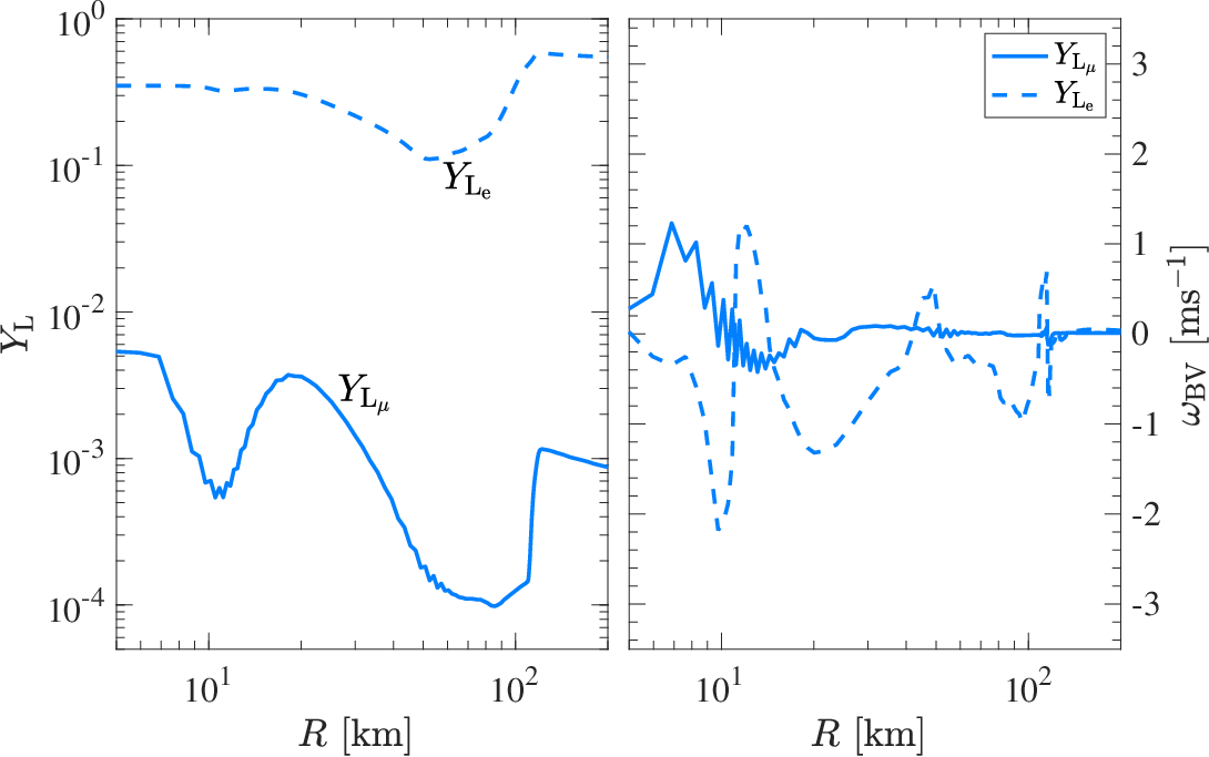
Since the present article’s concern is the impact of muons, and associated muonic weak processes, on the SN dynamics, the focus is on the lepton-number, , and the associated second term in Eq. (9); in particular, since it has been shown that the presence of muons has a negligible impact on the PNS structure and the entropy profile. Due to the separation of muonic and electronic lepton numbers, henceforth denoted as and , here the following question shall be addressed: Can a negative muonic lepton number gradient drive convection? Fig. 11 shows the lepton numbers (left panel) and the lepton-number gradient terms of (right panel), shortly after core bounce. Note that, in the case without muons and associated weak reactions that give rise to a finite muon abundance, the muonic lepton number is given by and, hence, suppressed by several orders of magnitude, such that its gradient is effectively zero. In contrast, here one can already identify shortly after core bounce the presence of the additional and non-negligible muon lepton number and associated contributions (solid lines in Fig. 11). The region with for corresponds to the PNS interior from intermediate to highest densities, on the order of g cm-3 to few times g cm-3 (see Fig. 8(b)), unlike for for which at lower densities, at the PNS surface. The region with for at large radii, between the SN shock and the PNS surface, is relevant for the development of convection. This is essential to the neutrino heating and cooling of matter in this region. The region with for indicates the occurance of convection in the PNS interior. It is interesting to note that the Ledoux-convection criterion has the same magnitude for and (see Fig. 11). This remains true during the entire post-bounce evolution. The magnitude of the impact remains to be determined in detailed multi-dimensional studies, preferably in three spatial dimensional simulations. This might have interesting implications for the emission of gravitational waves stemming from high densities Andresen et al. 2017; Kawahara et al. 2018; Morozova et al. 2018; Powell and Müller 2019; Radice et al. 2019; Mezzacappa et al. 2020.
V Summary
In the present article, the extension of AGILE-BOLTZTRAN to treat 6-species neutrino transport was introduced, overcoming the previous drawback of assuming equal – and –(anti)neutrino distributions. This enables a variety of muonic weak processes. These include muonic charged-current emission/absorption reactions involving the mean-field nucleons, as well as purely leptonic flavor-changing reactions. All these muonic rates have significant inelastic contributions. Hence, it is important to treat the corresponding phase space properly. In addition to the disentanglement of – and –(anti)neutrinos in the transport scheme, the presence of muonic weak processes gives rise to a finite and rising muon abundance. Therefore, together with its corresponding evolution equation, the muon abundance was added as an additional independent variable to the neutrino radiation-hydrodynamics state-vector of AGILE-BOLTZTRAN.
With these updates, stellar core collapse was simulated and studied in detail with a particular focus on the appearance of muons, muonic weak reactions, and possible consequences for SN phenomenology. It had been claimed previously that muons and their associated weak reactions may enhance the neutrino heating efficiency in multidimensional SN simulations under certain circumstances during the post-bounce evolution Bollig et al. 2017. Beginning with our first focus, muonization of SN matter, we find that it starts shortly before core bounce in two steps: first, from the production of high-energy muon-(anti)neutrinos from neutrino-pair processes, and second, from the absorption of these high-energy muon-neutrinos as part of the muonic charged-current and lepton-flavor changing processes. Here we conclude that the importance of the charged-current reactions exceed the latter by far for the muonization. We find that the muon abundance rises by more than one order of magnitude during the first few ten milliseconds post bounce, reaching values of to a few times – in particular, off center associated with the increasing temperature there. With regard to SN phenomenology: The presence of muons leads to a muon-neutrino burst shortly after core bounce, which is due to the shock propagation across the muon-neutrinosphere, similar to what happens with regard to the electron-neutrino burst when the shock passes the electron neutrinosphere. However, the muon-neutrino burst has a lower magnitude due to the significantly lower muon abundance and muonic charged-current weak rates, relative to the abundances and rates associated with electrons. With regard to the evolution of the PNS: It is interesting to note that muons and muon-(anti)neutrinos are not in weak equilibrium instantaneously, unlike the electrons and positrons with their neutrino species. That is, the electron chemical potentials by far exceed the muon chemical potentials at the PNS interior. Only towards low densities near the neutrinospheres at the PNS surface, where the abundance of trapped neutrinos drops to zero, are the electron and muon chemical potentials equal during the post-bounce evolution. It remains to be explored in future studies how the muons approach equilibrium during the later PNS deleptonization phase; i.e., after the onset of the SN explosion on a timescale of several ten seconds. Furthermore, the presence of an additional muon lepton-number gradient may impact convection at high densities in the PNS interior. To confirm this requires multidimensional simulations, which cannot be investigated here. We find that the presence of a finite and continuously rising muon abundance in the PNS interior has a softening impact on the high-density equation of state. This, in turn, is known to result in smaller PNS and shock radii during the long-term post-bounce supernova evolution on the order of several hundreds of milliseconds, confirming the findings of Ref. Bollig et al. 2017, which has the potential of enhancing the neutrino heating efficiency through higher neutrino energies and luminosities. The latter is also known from multidimensional simulations comparing stiff and soft hadronic equations of state Suwa et al. 2013. Moreover, the finite muon abundance may also give rise to weak processes involving pions Fore and Reddy 2020, which remains to be explored in future studies.

Acknowledgements.
T.F. acknowledges support from the Polish National Science Center (NCN) under grant No. 2016/23/B/ST2/00720 and No 2019/33/B/ST9/03059. G.M.P is partly supported by the Deutsche Forschungsgemeinschaft (DFG, German Research Foundation)—Project-ID 279384907— SFB 1245. A.M. acknowledges support from the National Science Foundation through grant NSF PHY 1806692. The SN simulations were performed at the Wroclaw Center for Scientific Computing and Networking (WCSS) in Wroclaw (Poland).Appendix A AGILE-BOLTZTRAN – Extension to 6-species Boltzmann neutrino transport
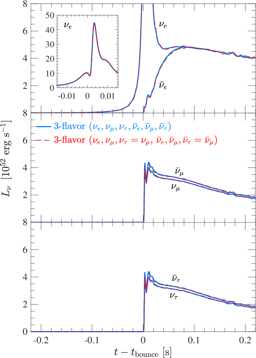
Here, a comparison is presented between the reference run employing the 6-species neutrino transport scheme (blue lines) and the run based on the traditional 4-species (red lines), where besides the inclusion of electron and muon neutrino flavors it is assumed that the tau-(anti)neutrino distributions are equal to the muon-(anti)neutrino distributions. No muonic weak processes are considered here. All muonic weak rates are set (numerically) to zero.
Fig. 12 compares the evolution of the neutrino luminosities in Fig. 12(a) and the average neutrino energies in Fig. 12(b) for the two SN simulations, respectively. Otherwise, both simulations employ an identical set of input physics, as introduced in Secs. II.1 and II.2. The relative change between the two runs in terms of neutrino losses is on the order of less than a few tenths of one percent, attributed mostly to a slightly different converged solution of the radiation-hydrodynamics equations Liebendörfer et al. 2004 with the implementation of the muon abundance as additional independent degree of freedom. Furthermore, the entire SN hydrodynamics – i.e., shock formation, shock evolution, and post-bounce mass accretion – shows no quantitative differences.
Appendix B Implementation of muonic weak processes
B.1 Muonic charged-current processes – elastic rates
The CC rates within the full kinematics approach, including self-consistent contributions from weak magnetism, are provided in Ref. Fischer et al. 2020b for the electronic CC processes. They have been reviewed recently for the muonic reactions (1a) and (1b) of Table 1 in Ref. Guo et al. 2020. For the comparison with this full kinematics treatment, it is convenient to provide CC muonic rates in the elastic approximation; i.e., assuming a zero-momentum transfer, for which the absorptivity () is given by the following analytical expression:
| (11) |
with Fermi constant, , vector and axial-vector coupling constants, and , as well as with equilibrium Fermi–Dirac distribution functions for the muons, , neutron/proton number densities, and the latter free Fermi gas chemical potentials, and , respectively. The latter are related to the nuclear EOS chemical potentials, , as follows: , with neutron/proton single-particle vector-interaction potentials and effective masses Martínez-Pinedo et al. 2012; Roberts et al. 2012a, both of which are given by the nuclear EOS. Inelastic contributions and weak-magnetism corrections are approximately taken into account via neutrino-energy-dependent multiplicative factors to the emissivity and opacity Horowitz 2002. A similar expression as (11) is obtained for by replacing the muon Fermi distribution with that of anti-muons and replacing for the neutron/proton number densities and free gas chemical potentials.
The emissivity and absorptivity are related intimately via detailed balance,
| (12) |
with muon-neutrino equilibrium chemical potential given by the expression, .
For this limited kinematics assuming zero-momentum transfer, one can relate the muon and energies as follows,
| (13) |
with the medium-modified value, Reddy et al. 1998; Martínez-Pinedo et al. 2012; Roberts et al. 2012a. Note that, as for the electron-flavor neutrinos, the nuclear medium modifications for the charged-current rate at the mean-field level modify the opacity substantially with increasing density Martínez-Pinedo et al. 2014. In particular, at densities in excess of g cm-3, where muons can be expected, the opacity drop can differ significantly from the vacuum value, due to the large difference of the single particle potentials can well be on the order of MeV, depending on the nuclear EOS Fischer et al. 2014; Martínez-Pinedo et al. 2014.
The presence of high-energy and enables the production of . The collision integrals for and for the reactions (1a) and (1b) of Table 1 take the following form:
with effective opacity defined as follows, Mezzacappa and Bruenn 1993a; Mezzacappa and Bruenn 1993b. Expressions () and () are equivalent to those for the electron-(anti)neutrinos with electronic charged-current emissivity and opacity Fischer et al. 2012. The muon abundance, , is then added as an independent variable to the AGILE state vector, for which the following differential-integral evolution equation is solved,
| (16) |
with baryon mass MeV. Equation (16) is similar to the evolution equation for (see Eqs. (17)–(25) in Ref. Mezzacappa and Bruenn 1993b), where, instead, the electronic charged-current neutrino emissivity and opacity are used (see expressions (6) and (7a)–(7d) in Ref. Fischer et al. 2012).
B.2 Neutrino-muon scattering
For neutrino–lepton scattering (NLS), , distinguishing here between neutrinos, , and leptons, , the collision integral is given by the following integral expression,
| (17) | |||||
with the following definition for the in- and out-scattering kernels,
| (18) | |||
| (19) |
with equilibrium Fermi-Dirac distribution functions for initial- and final-state leptons. In addition to the energy difference between incoming and outgoing neutrinos, , the scattering kernels depend on the total momentum scattering angle between the incoming and outgoing neutrino, defined as follows,
| (20) |
with lateral momentum angles and relative azimuthal angle (for illustration, see Fig. (1) in Ref Mezzacappa and Bruenn 1993a).
Here, for neutrino–muon scattering (NMS), the approach for neutrino–electron scattering (NES) is extended following the Refs. Tubbs and Schramm 1975; Schinder and Shapiro 1982; Bruenn 1985; Mezzacappa and Bruenn 1993. As an example, in the following neutrino–muon scattering, , will be considered, which contains neutral-current -boson and charged-current -boson interactions, similar to scattering (see Fig. 1 in Ref. Tubbs and Schramm 1975). The matrix element, , for scatteringa can be obtained from the literature, cf. Eqs. (C46)–C(48) in Ref. Bruenn 1985, by replacing the electron and spinors, , with those of the muon and , , respectievely,
| (21) |
The matrix element depends on the particle’s 4-momenta, , and the dash denotes final states. The quantities and are the vector and axial-vector coupling constants. After spin-averaging and squaring, the transition amplitude takes the following form,
| (22) | |||
| (23) |
with , and , where the values for and are listed in Table 3.
The individual kinematic integral expression, denoted as , which correspond to the muon initial- and final-state momentum integrals of , can be obtained from Eq. (10b) in Ref. Tubbs and Schramm 1975 by replacing the electron with the muon 4-momenta. The remaining integrals are solved numerically following the approach developed in Ref. Mezzacappa and Bruenn 1993 for neutrino-electron scattering, such that
| (24) |
The definition of the remaining integrals, , is given in Eqs. (11)–(27) in Ref. Mezzacappa and Bruenn 1993, based on the polylogarithm functionals, which are used to perform the remaining Fermi-integrals.
In order to eliminate the remaining dependence on the relative azimuthal angle in the scattering kernels (18) and (19), a numerical 32-point Gauss quadrature integration is employed, which is identical to the one of BOLTZTRAN for neutrino–electron scattering (see Eq. (32) in Ref. Mezzacappa and Bruenn 1993), such that the scattering kernels depend only on incoming and outgoing neutrino energies, as well as on the incoming and outgoing neutrino lateral angles, . For the procedure to avoid singular forward scattering, expressions (37)–(43) in Ref. Mezzacappa and Bruenn 1993 are employed here for neutrino–muon scattering.
For muon-antineutrino scattering on muons the expressions are a cross channel of muon–neutrino scattering introduced above (similar to the relationship between electron-antineutrino scattering on electrons and electron-neutrino scattering on electrons Bruenn 1985), given by the substitution in the matrix element. It has been realized for neutrino–electron scattering, this corresponds to the replacement of in the expressions for the scattering kernels Bruenn 1985. Therefore, it is straightforward to obtain the corresponding scattering kernel . Similar replacements are done for electron-(anti) neutrino scattering on muons, Bruenn 1985. Table 3 summarizes the values of and for all neutrino-(anti)muon scattering reactions. Furthermore, since the collision integral of the Boltzmann equation (17) has an identical form for NMS and NES, the general neutrino–lepton scattering kernel in the module for the inelastic scattering processes of Boltztran is defined as follows,
| (25) |
for each pair of neutrino specie .
Note that, due to detailed balance, the transition amplitudes for in- and out-scattering are equal, (the degeneracy factors cancel), such that the scattering kernels (18) and (19) are related via,
| (26) |
which is the case for both, NES and NMS.
B.3 Purely leptonic lepton flavor changing processes
B.3.1 Lepton flavor exchange (LFE)
As an example, in the following the focus will be on the the reaction: . In close analogy to (17), the collision integral of the Boltzmann transport equation is given by the following integral expression,
| (27) |
with the in- and out-scattering kernels, again in close analogy to (18) and (19), given as follows,
| (28) | |||||
| (29) | |||||
The similarity to the expressions for neutrino–muon scattering, introduced above, is striking. However, unlike – scattering which has neutral-current -boson and charged-current -boson contributions, this process is given by a -boson exchange only, with the following matrix element:
| (30) |
with the spinors, , depending on the corresponding 4-momenta, , where the dash denotes final states. After summation and spin-averaging, the transition amplitude takes the following form,
| (31) |
such that,
| (32) |
with the same definition of the remaining phase-space integral as for the case of neutrino–muon scattering discussed above. However, due to different initial-state electron and final-state muon rest masses, there are additional terms, which scale with the rest-mass energy difference, . Comparing these terms with those for neutrino–muon scattering (see Eqs. (11)–(18) in Ref. Mezzacappa and Bruenn 1993) and using the same nomenclature as in Ref. Mezzacappa and Bruenn 1993, the following modifications arise,
| (33) |
The functions , , , , , as well as the integral functionals , are defined in Ref. Mezzacappa and Bruenn 1993, see Eqs. (14)–(20). The latter are related to the Fermi integrals, which depend on the degeneracy parameter, , which is related to , and defined as follows,
| (34) |
in contrast to Eq. (22) in Ref. Mezzacappa and Bruenn 1993, since electrons and muons can have rather different Fermi energies under SN conditions. Furthermore, the argument, , of the Fermi-integrals, , also has an explicit dependence on the electron–muon rest-mass energy difference as follows,
| (35) | |||||
The additional phase-space terms, , and , are given by the following expressions,
| (36) | |||||
| (37) | |||||
| (38) |
Note also, in order to eliminate the azimuthal dependence of the scattering kernels, the same 32-point Gauss quadrature numerical integration is performed as in the case of neutrino–lepton scattering. Note further that the relation of detailed balance holds here as well for the transition amplitudes of the lepton-flavor exchange processes. However, due to the presence of two different leptonic chemical potentials, the phase-space distributions for electrons and muons give rise to an additional contribution to the relation of detailed balance for the scattering kernels, as follows,
| (39) |
Note that, since the transition amplitudes for the processes involving and are the same as for the processes involving and , the scattering kernels are given by the same expression (33), with the replacement of the chemical potentials, , and .
For the implementation of the LFE processes, (3a) and (3b) in Table 1, in the collision integral, the scattering kernels are computed on the fly as part of the inelastic scattering module of BOLTZTRAN. However, contrary to neutrino–lepton scattering, here the initial- and final-state neutrinos belong to different flavors. A new module for this class of inelastic processes had to be introduced according to (27), for (anti)muon- and (anti)electron-neutrinos.
B.3.2 Lepton flavor conversion (LFC)
For LFC reactions (4a) and (4b) of Table 1, the collision integral of the Boltzmann equation takes the same form as (27), though changing initial- and final-state neutrino distributions respectively. Also in- and out-scattering kernels have the same algebraic structure as for the lepton flavor exchange processes (28) and (29), i.e. converting (positron)electron into (anti)muon and vize versa. However, the matrix elements for LFC reactions are different.
In the following, the process, , will be discussed as an example, for which the matrix element can be directly read off from (31), replacing the spinor with that of neutrino and the spinor with that of neutrino. Then, the transition amplitude takes the following form,
| (40) |
such that the out-scattering kernel becomes,
with the same remaining phase-space integral, , as for the case of neutrino–muon scattering discussed above (see also Eq. (12) in Ref. Mezzacappa and Bruenn 1993), with the replacements and , as well as the inclusion of the muon-electron rest-mass energy scale . Then, applying the same nomenclature as in Ref. Mezzacappa and Bruenn 1993 and as in (33), the resulting additional terms, , , and , can be computed straightforwardly with the aforementioned replacements. Note that the scattering kernels for the processes involving and are obtained by the replacement of the chemical potentials as follows, .
Since in- and out-scattering LFC kernels have the same algebraic structure as in- and out-scattering LFE kernels, respectively, the reverse LFC processes are related through detailed balance in the same way the LFE kernels are (39). Hence, it is convenient to define the total lepton flavor exchange/conversion scattering kernel,
| (42) |
Note that LFE and LFC reactions change the abundance of muons and electrons. Their contributions have to be taken into account by modifying the evolution equations () and () as follows,
| (43) | |||
Similarly, the evolution equation has to be modified, as well,
| (44) | |||
References
- Janka et al. (2007) H.-T. Janka, K. Langanke, A. Marek, G. Martínez-Pinedo, and B. Müller, Phys. Rep. 442, 38 (2007).
- Janka (2012) H.-T. Janka, Ann. Rev. of Nucl. Part. Sci. 62, 407 (2012).
- Bethe and Wilson (1985) H. A. Bethe and R. Wilson, James, Astrophys. J. 295, 14 (1985).
- LeBlanc and Wilson (1970) J. M. LeBlanc and J. R. Wilson, Astrophys.J. 161, 541 (1970).
- Burrows et al. (2006) A. Burrows, E. Livne, L. Dessart, C. Ott, and J. Murphy, Astrophys. J. 640, 878 (2006).
- Sagert et al. (2009) I. Sagert, T. Fischer, M. Hempel, G. Pagliara, J. Schaffner-Bielich, et al., Phys. Rev. Lett. 102, 081101 (2009).
- Fischer et al. (2018) T. Fischer, N.-U. F. Bastian, M.-R. Wu, P. Baklanov, E. Sorokina, S. Blinnikov, S. Typel, T. Klähn, and D. B. Blaschke, Nat. Astron. 2, 980 (2018).
- Fischer et al. (2020a) T. Fischer, M.-R. Wu, B. Wehmeyer, N.-U. F. Bastian, G. Martínez-Pinedo, and F.-K. Thielemann, Astrophys. J. 894, 9 (2020a).
- Müller (2016) B. Müller, Publ. Astron. Soc. Austr. 33, e048 (2016).
- Fischer et al. (2017) T. Fischer, N.-U. Bastian, D. Blaschke, M. Cierniak, M. Hempel, T. Klähn, G. Martínez-Pinedo, W. G. Newton, G. Röpke, and S. Typel, Publ. Astron. Soc. Austr. 34, e067 (2017).
- Yamada et al. (1999) S. Yamada, H.-T. Janka, and H. Suzuki, Astron.Astrophys. 344, 533 (1999), arXiv:astro-ph/9809009 [astro-ph] .
- Liebendörfer et al. (2001) M. Liebendörfer, A. Mezzacappa, F.-K. Thielemann, O. B. Messer, W. R. Hix, et al., Phys. Rev. D 63, 103004 (2001).
- Chan and Müller (2020) C. Chan and B. Müller, Month. Not. Roy. Astron. Soc. 496, 2000 (2020).
- Ott et al. (2008) C. D. Ott, A. Burrows, L. Dessart, and E. Livne, Astrophys. J. 685, 1069 (2008).
- Nagakura et al. (2018) H. Nagakura, W. Iwakami, S. Furusawa, H. Okawa, A. Harada, K. Sumiyoshi, S. Yamada, H. Matsufuru, and A. Imakura, Astrophys. J. 854, 136 (2018).
- Glendenning (1996) N. Glendenning, in Compact Stars. Nuclear Physics, Particle Physics and General Relativity (1996).
- Bollig et al. (2017) R. Bollig, H.-T. Janka, A. Lohs, G. Martínez-Pinedo, C. J. Horowitz, and T. Melson, Phys. Rev. Lett. 119, 242702 (2017).
- Bollig et al. (2020) R. Bollig, W. DeRocco, P. W. Graham, and H.-T. Janka, Phys. Rev. Lett. 125, 051104 (2020).
- Mezzacappa and Bruenn (1993a) A. Mezzacappa and S. Bruenn, Astrophys. J. 405, 669 (1993a).
- Mezzacappa and Bruenn (1993b) A. Mezzacappa and S. Bruenn, Astrophys. J. 405, 637 (1993b).
- Mezzacappa and Bruenn (1993) A. Mezzacappa and S. W. Bruenn, Astrophys. J. 410, 740 (1993).
- Liebendörfer et al. (2001) M. Liebendörfer, A. Mezzacappa, and F.-K. Thielemann, Phys. Rev. D 63, 104003 (2001).
- Liebendörfer et al. (2004) M. Liebendörfer, O. Messer, A. Mezzacappa, S. Bruenn, C. Cardall, et al., Astrophys. J. Suppl. 150, 263 (2004).
- Liebendörfer et al. (2002) M. Liebendörfer, S. Rosswog, and F.-K. Thielemann, Astrophys. J. Suppl. 141, 229 (2002).
- O’Connor et al. (2018) E. O’Connor, R. Bollig, A. Burrows, S. Couch, T. Fischer, H.-T. Janka, K. Kotake, E. J. Lentz, M. Liebendörfer, O. E. B. Messer, A. Mezzacappa, T. Takiwaki, and D. Vartanyan, J. Phys. G Nucl. Phys. 45, 104001 (2018).
- Hempel et al. (2012) M. Hempel, T. Fischer, J. Schaffner-Bielich, and M. Liebendörfer, Astrophys. J. 748, 70 (2012).
- Timmes and Arnett (1999) F. X. Timmes and D. Arnett, Astrophys. J. Suppl. 125, 277 (1999).
- Hempel and Schaffner-Bielich (2010) M. Hempel and J. Schaffner-Bielich, Nucl.Phys. A837, 210 (2010).
- Typel et al. (2010) S. Typel, G. Röpke, T. Klähn, D. Blaschke, and H. Wolter, Phys.Rev. C81, 015803 (2010).
- Buras et al. (2006) R. Buras, M. Rampp, H.-T. Janka, and K. Kifonidis, Astron. Astrophys. 447, 1049 (2006).
- Fischer et al. (2009) T. Fischer, S. C. Whitehouse, A. Mezzacappa, F.-K. Thielemann, and M. Liebendörfer, Astron. Astrophys. 499, 1 (2009).
- (32) is used here and not as in the standard literature, not to confuse with the muons.
- Bruenn (1985) S. W. Bruenn, Astrophys. J. Suppl. 58, 771 (1985).
- Guo et al. (2020) G. Guo, G. Martínez-Pinedo, A. Lohs, and T. Fischer, Phys. Rev. D 102, 023037 (2020).
- Fischer et al. (2020b) T. Fischer, G. Guo, A. A. Dzhioev, G. Martínez-Pinedo, M.-R. Wu, A. Lohs, and Y.-Z. Qian, Phys. Rev. C 101, 025804 (2020b).
- Oertel et al. (2020) M. Oertel, A. Pascal, M. Mancini, and J. Novak, arXiv e-prints , arXiv:2003.02152 (2020), arXiv:2003.02152 [astro-ph.HE] .
- Horowitz (2002) C. Horowitz, Phys. Rev. D 65, 043001 (2002).
- Tubbs and Schramm (1975) D. Tubbs and D. Schramm, Astrophys. J. 201, 467 (1975).
- Schinder and Shapiro (1982) P. J. Schinder and S. L. Shapiro, Astrophys. J. Suppl. 50, 23 (1982).
- Fischer et al. (2012) T. Fischer, G. Martínez-Pinedo, M. Hempel, and M. Liebendörfer, Phys. Rev. D 85, 083003 (2012).
- Woosley et al. (2002) S. Woosley, A. Heger, and T. Weaver, Rev. Mod. Phys. 74, 1015 (2002).
- Juodagalvis et al. (2010) A. Juodagalvis, K. Langanke, W. R. Hix, G. Martínez-Pinedo, and J. M. Sampaio, Nucl. Phys. A 848, 454 (2010).
- Martínez-Pinedo et al. (2012) G. Martínez-Pinedo, T. Fischer, A. Lohs, and L. Huther, Phys. Rev. Lett. 109, 251104 (2012).
- Roberts et al. (2012a) L. F. Roberts, S. Reddy, and G. Shen, Phys. Rev. C 86, 065803 (2012a).
- Fischer (2016) T. Fischer, Astron. Astrophys. 593, A103 (2016).
- Lentz et al. (2012) E. J. Lentz, A. Mezzacappa, O. E. B. Messer, M. Liebendörfer, W. R. Hix, and S. W. Bruenn, Astrophys. J. 747, 73 (2012).
- Kotake et al. (2018) K. Kotake, T. Takiwaki, T. Fischer, K. Nakamura, and G. Martínez-Pinedo, Astrophys. J. 853, 170 (2018).
- Wilson and Mayle (1988) J. R. Wilson and R. W. Mayle, Phys. Rep. 163, 63 (1988).
- Keil et al. (1996) W. Keil, H. Janka, and E. Muller, Astrophys. J. 473, L111 (1996).
- Kotake et al. (2006) K. Kotake, K. Sato, and K. Takahashi, Rept. Prog. Phys. 69, 971 (2006).
- Roberts et al. (2012b) L. F. Roberts, G. Shen, V. Cirigliano, J. A. Pons, S. Reddy, and S. E. Woosley, Phys. Rev. Lett. 108, 061103 (2012b).
- Mirizzi et al. (2016) A. Mirizzi, I. Tamborra, H.-T. Janka, N. Saviano, K. Scholberg, R. Bollig, L. Hüdepohl, and S. Chakraborty, Nuovo Cimento Rivista Serie 39, 1 (2016).
- Andresen et al. (2017) H. Andresen, B. Müller, E. Müller, and H. T. Janka, Month. Not. Roy. Astron. Soc. 468, 2032 (2017).
- Kawahara et al. (2018) H. Kawahara, T. Kuroda, T. Takiwaki, K. Hayama, and K. Kotake, Astrophys. J. 867, 126 (2018).
- Morozova et al. (2018) V. Morozova, D. Radice, A. Burrows, and D. Vartanyan, Astrophys. J. 861, 10 (2018).
- Powell and Müller (2019) J. Powell and B. Müller, Month. Not. Roy. Astron. Soc. 487, 1178 (2019).
- Radice et al. (2019) D. Radice, V. Morozova, A. Burrows, D. Vartanyan, and H. Nagakura, Astrophys. J. 876, L9 (2019).
- Mezzacappa et al. (2020) A. Mezzacappa, P. Marronetti, R. E. Landfield, E. J. Lentz, K. N. Yakunin, S. W. Bruenn, W. R. Hix, O. E. B. Messer, E. Endeve, J. M. Blondin, and J. A. Harris, Phys. Rev. D 102, 023027 (2020).
- Suwa et al. (2013) Y. Suwa, T. Takiwaki, K. Kotake, T. Fischer, M. Liebendörfer, and K. Sato, Astrophys. J. 764, 99 (2013).
- Fore and Reddy (2020) B. Fore and S. Reddy, Phys. Rev. C 101, 035809 (2020).
- Reddy et al. (1998) S. Reddy, M. Prakash, and J. M. Lattimer, Phys. Rev. D 58, 013009 (1998).
- Martínez-Pinedo et al. (2014) G. Martínez-Pinedo, T. Fischer, and L. Huther, J. Phys. G Nucl. Part. Phys. 41, 044008 (2014).
- Fischer et al. (2014) T. Fischer, M. Hempel, I. Sagert, Y. Suwa, and J. Schaffner-Bielich, Eur. Phys. J. A 50, 46 (2014).