-Cores: Robust Large-Scale Bayesian Data Summarization in the Presence of Outliers
Abstract
Modern machine learning applications should be able to address the intrinsic challenges arising over inference on massive real-world datasets, including scalability and robustness to outliers. Despite the multiple benefits of Bayesian methods (such as uncertainty-aware predictions, incorporation of experts knowledge, and hierarchical modeling), the quality of classic Bayesian inference depends critically on whether observations conform with the assumed data generating model, which is impossible to guarantee in practice. In this work, we propose a variational inference method that, in a principled way, can simultaneously scale to large datasets, and robustify the inferred posterior with respect to the existence of outliers in the observed data. Reformulating Bayes theorem via the -divergence, we posit a robustified pseudo-Bayesian posterior as the target of inference. Moreover, relying on the recent formulations of Riemannian coresets for scalable Bayesian inference, we propose a sparse variational approximation of the robustified posterior and an efficient stochastic black-box algorithm to construct it. Overall our method allows releasing cleansed data summaries that can be applied broadly in scenarios including structured data corruption. We illustrate the applicability of our approach in diverse simulated and real datasets, and various statistical models, including Gaussian mean inference, logistic and neural linear regression, demonstrating its superiority to existing Bayesian summarization methods in the presence of outliers.
Index terms— Scalable learning; Big data summarizations; Coresets; Variational inference; Robust statistics; Noisy observations; Data valuation
1 Introduction
Machine learning systems perpetually collect growing datasets, such as product reviews, posting activity on social media, users feedback on services, or insurance claims. The rich information content of such datasets has opened up an exciting potential to tackle various practical problems. Hence, recent years have witnessed a surge of interest in scaling up inference in the large-data regime via stochastic and batch methods [1, 23, 56]. Most of related approaches have treated datapoints indiscriminantly; nevertheless, it is well known that not all datapoints contribute equally valuable information for a given target task [21].
Datasets collected in modern applications contain redundant input samples that reflect very similar statistical patterns, or multiple copies of identical observations. Often input aggregates subpopulations emanating from different distributions [60, 61]. Moreover, the presence of outliers is a ubiquitous challenge, attributed to multiple causes. In the first place, noise is inherent in most real-world data collection procedures, creating systematic outliers: crowdsourcing is prone to mislabeling [18] and necessitates laborious data cleansing [33, 39], while measurements commonly capture sensing errors and system failures. Secondly, outliers can be generated intentionally from information contributing parties, who aim to compromise the functionality of the application through data poisoning attacks [2, 6, 34, 31, 48, 21], realised for example via data generation from fake accounts. Outliers detection is challenging, particularly in high dimensions [13, 14]. Proposed solutions often are model-specific, and include dedicated learning components which increase the time complexity of the application, involve extensive hyperparameter tuning, introduce data redundancies, or require model retraining [46, 57, 41, 29, 35, 59]. On the other hand, operating on a corrupted dataset is brittle, and can decisively degrade the predictive performance of downstream statistical tasks, deceptively underestimate model uncertainty and lead to incorrect decisions.
In this work, we design an integrated approach for inference on massive scale observations that can jointly address scalability and data cleansing for complex Bayesian models, via robust data summarization. Our method inherits the full set of benefits of Bayesian inference and works for any model with tractable likelihood function. At the same time, it maintains a high degree of automation with no need for manual data inspection, no additional computational overhead due to robustification, and can tolerate a non-constant number of corruptions. Moreover, our work points to a more efficient practice in large-scale data acquisition, filtering away less valuable samples, and indicating the regions of the data space that are most beneficial for our inference task.
Our solution can be regarded as an extension of Bayesian coreset methods that can encompass robustified inference. Bayesian coresets [27, 8, 7] have been recently proposed as a method that enables Bayesian learning at scale via substituting the complete dataset over inference with an informative sparse subset thereof. Robustified Bayesian inference methods [4] have sought solutions to mismatches between available observations and the assumed data generating model, via proposing heavy-tailed data likelihood functions [26, 42] and localization [12, 52], using robust statistical divergences [20, 30, 38], employing robust gradient estimates over Langevin Monte Carlo methods [5], or inferring datapoints-specific importance weights [54]. Here, we cast coreset construction in the framework of robustified inference, introducing -Cores, a method that learns sparse variational approximations of the full data posterior under the -divergence. In this way, we are able to yield summaries of large data that are distilled from outliers, or data subpopulations departing from our statistical model assumptions. Importantly, -Cores can act as a preprocessing step, and the learned data summaries can subsequently be given as input to any ordinary or robustified black-box inference algorithm.
The rest of this paper is organized as follows. In Sections 2 and 3 we introduce necessary concepts from Bayesian inference, and present our proposed method. In Section 4 we expose experimental results on simulated and real-world benchmark datasets: we consider diverse statistical models and scenarios of extensive data contamination, and demonstrate that, in contrast to existing summarization algorithms, our method is able to maintain reliable predictive performance in the presence of structured and unstructured outliers. Finally, in Section 5 we provide conclusions and discuss future works.
2 Preliminaries
In this section, we introduce the required concepts from Bayesian inference, present robustness limitations of standard posterior on big data, and outline existing generalizations of the posterior that aim to robustify inference with respect to data mismatch.
2.1 Standard Bayesian inference and lack of robustness in the large-data regime
In the context of Bayesian inference, we are interested in updating our beliefs about a vector of random variables , initially expressed through a prior distribution , after observing a set of datapoints . Posterior on can be computed via the application of Bayes rule
| (1) |
where is a (typically intractable) normalization constant, and is the likelihood of our observations according to an assumed statistical model. When datapoints are conditionally independent given —which is the primary focus of this work—likelihood gets factorized as . An equivalent formulation of the Bayesian posterior as a solution to an optimization problem was proposed by Zellner [58], which is written as
| (2) |
In the above, is the empirical distribution of the observed datapoints. The exponent corresponds (up to a constant) to the cross-entropy, which is equal to the empirical average of negative log-likelihoods of the datapoints, and quantifies the expected loss incurred by our estimates for the model parameters over the available observations, under the Kullback-Leibler (KL) divergence.
When is large, the Bayesian posterior is strongly affected by perturbations in the observed data space. To develop an intuition on this, assuming that the true and observed data distributions have densities and respectively, we can rewrite an approximation of Eq. 2 via the KL divergence () as [38]
| (3) | ||||
| (4) |
where denotes agreement to first order in exponent.†† † i.e. iff Hence, due to the large in the exponent, small changes to will have a large impact on the posterior.
2.2 Robustified posteriors
Robust inference methods aim to adapt Eq. 1 to formulations that can address the case of observations departing from model assumptions, as often happening in practice, e.g. due to misspecified shapes of data distributions and number of components, or due to the presence of outliers. In such formulations [11, 28, 19, 17], Bayesian updates rely on utilising robust divergences instead of the KL divergence, to express the losses over the data.
A popular choice [20, 30] for enhancing robustness of inference is replacing the log-likelihood terms arising in Eq. 2 with the -divergence (or density power divergence) [3, 10], which yields the following posterior for [22, 30]
| (5) |
where
| (6) |
with . We refer to quantities defined in Eqs. 5 and 6 as the -posterior and -likelihood respectively. Noticeably, the individual terms of the -likelihood allow attributing different strength of influence to each of the datapoints, depending on their accordance with the model assumptions. As densities get raised to a suitable power , outlying observations are exponentially downweighted. When , Eq. 2 is recovered and all datapoints are treated equally.
In the presentation above we focused on modeling observations (unsupervised learning). In the case of supervised learning on data pairs , the respective expression for individual terms of -likelihood‡‡ ‡ In this context for simplicity we use notation to denote . is [3]
| (7) |
3 Method
In this section we discuss -Cores, our unified solution to the robustness and scalability challenges of large-scale Bayesian inference. Section 3.1 introduces the main quantity of interest in our inference method, and shows how it addresses the exposed issues. Section 3.2 presents an iterative algorithm that allows efficient approximate computations of our posterior.
3.1 Sparse -posterior
Scaling up the computation of Eq. 5 in the regime of massive datasets for non-conjugate models is challenging: similarly to Eq. 1, applying Markov chain Monte Carlo (MCMC) methods to sample from the -posterior, implies a computational cost scaling at order .
Bayesian coresets [27, 8] have been recently proposed as a method to circumvent the computational cost for the purposes of approximate inference via summarizing the original dataset with a small learnable subset of weighted datapoints , where . Substituting Eq. 6 in Eq. 5, allows us to explicitly introduce a weights vector in the posterior, and rewrite the latter in the general form
| (8) |
In the case of the -posterior on the full dataset Eq. 5, we have ; for coreset posteriors this vector acts as a learnable parameter and attains a non-trivial sparse value, with non-zero entries corresponding to the elements of the full dataset that are selected over the summarization.
Although Bayesian coresets can dramatically reduce inference time, they inherit the susceptibility of Bayesian posterior to data mismatch in the large data regime: even though the number of points used in inference gets reduced, these points are now weighted, hence the remark of Eq. 4 can carry over in coresets posterior.
The recent formulation of Riemannian coresets [7] has framed the problem of coreset construction as Variational Inference (VI) in a sparse exponential family. Our method provides a natural extension of this framework to robust divergences. Here we aim to approximate data posterior via a sparse -posterior, which can be expressed as follows
| (9) |
In the following we denote expectations and covariances under as and respectively. Then the KL divergence is written as
| (10) |
In our formulation it is easy to observe that posteriors of Eq. 8 form a set of exponential family distributions [51], with natural parameters , sufficient statistics , and log-partition function . Following [7], the objective can be expanded as
| (11) | ||||
| (12) |
and minimized via gradient descent on . The gradient of the objective of Eq. 12 can be derived in closed form, as
| (13) |
where .
3.2 Black-box stochastic scheme for incremental coreset construction
To scale up coreset construction on massive datasets we use stochastic gradient descent on minibatches , with . The covariance of Eq. 13 required for exact gradient computation of the variational objective is generally not available in analytical form. Hence, for our black-box coreset construction we approximate this quantity via Monte Carlo estimates, using samples of the unknown parameters from the coreset posterior. These samples can be efficiently obtained with complexity (not scaling with dataset size ) due to the sparsity of the coreset posterior over the procedure. The proposed black-box construction makes no assumptions on the statistical model other than having tractable -likelihoods. We employ a two-step incremental scheme, with complexity of order , where is the number of samples from the coreset posterior, and is the total number of iterations over coreset points weights optimization. The full incremental construction is outlined in Algorithm 1.
3.2.1 Next datapoint selection
We first select the next datapoint to include in our coreset summary, via a greedy selection criterion. Although maximizing decrease in KL locally via Eq. 13, seems to be the natural greedy choice here, using the information-geometric argument presented in [7], we use instead the following correlation maximization criterion:
| (14) |
where we denoted by the set of coreset points. The correlations for coreset and minibatch datapoints are empirically approximated as in lines 12 and 13 of Algorithm 1 respectively.
3.2.2 Coreset points reweighting
After adding a new datapoint we update the coreset weight vector via steps of projected stochastic gradient descent, using the Monte Carlo estimate of Eq. 13 per line 25 of Algorithm 1.
Summarization of observations groups and batches. Apart from working at the individual datapoints level, our scheme also enables summarizing batches and groups of observations. Acquiring efficiently informative batches of datapoints can replace random minibatch selection commonly used in stochastic optimization for large-scale model training. This extension can also be quite useful in situations where datapoints are partitioned in clusters, e.g. according to demographic information. For example, when gender and age features are available in datasets capturing users movies habits, collected datapoints can be binned accordingly, and our group summarization technique will allow extracting informative combinations of demographic groups that can jointly summarize the entire population’s information. The robustness properties of -Cores in such applications can aid removing group bias, and rejecting groups with large fractions of outliers. Algorithm 1 is again directly applicable, where vectors are now summed over the corresponding datapoints of each batch or group.
4 Experiments & Applications
We examine the inferential results achieved by our method under 3 statistical models, in scenarios capturing different types of data mismatch with reality. The data contamination models used in following experiments are reminiscent of Huber’s -contamination model [25], which postulates that observed data are generated from a mixture of distributions of the form , where , is a distribution of inliers captured by the assumed statistical model, and is an arbitrary distribution of outliers. This model has found use in several recent studies on robust statistical estimators suitable for underlying distributions with minimal assumptions [55, 9].
-Cores is compared against a uniformly random sampling baseline, and stochastic batch implementations of two existing Riemannian coreset methods:
- (i)
SparseVI [7], which builds up a coreset according to an incremental scheme similar to ours, considering the standard likelihood function terms evaluated on the dataset points, and
- (ii)
PSVI [37], which runs a batch optimization on a set of pseudopoints, and uses standard likelihood evaluations to jointly learn the pseudopoints weights and locations so that the extracted summary resembles the statistics of the full dataset.
We default the number of iterations in the optimization loop over gradient-based coreset constructions to , using a learning rate and random projections per gradient computation. For consistency with the compared baselines, we evaluate inference results obtained by -Cores using the classical Bayesian posterior from Eq. 1 conditioned on the corresponding robustified data summary. Additional details on used benchmark datasets are presented in Appendix B. Code is available at https://github.com/dionman/beta-cores.
4.1 Simulated Gaussian Mean Inference under Stuctured Data Contamination
In this experiment we study how -Cores behaves in the setting of mean inference on synthetic -dimensional data, sampled i.i.d. from a normal distribution with known covariance,
| (15) |
In the presented results, we use priors and , dimensionality and dataset size .
We consider the case of structured data corruption existing in the observations, simulated as follows: Observed datapoints are typically sampled from a Gaussian . At a percentage , data collection fails; in this case, datapoints are collected from a shifted Gaussian . Consequently, the observed dataset forms a Gaussian mixture with two components; however, our statistical model assumes only a single Gaussian.
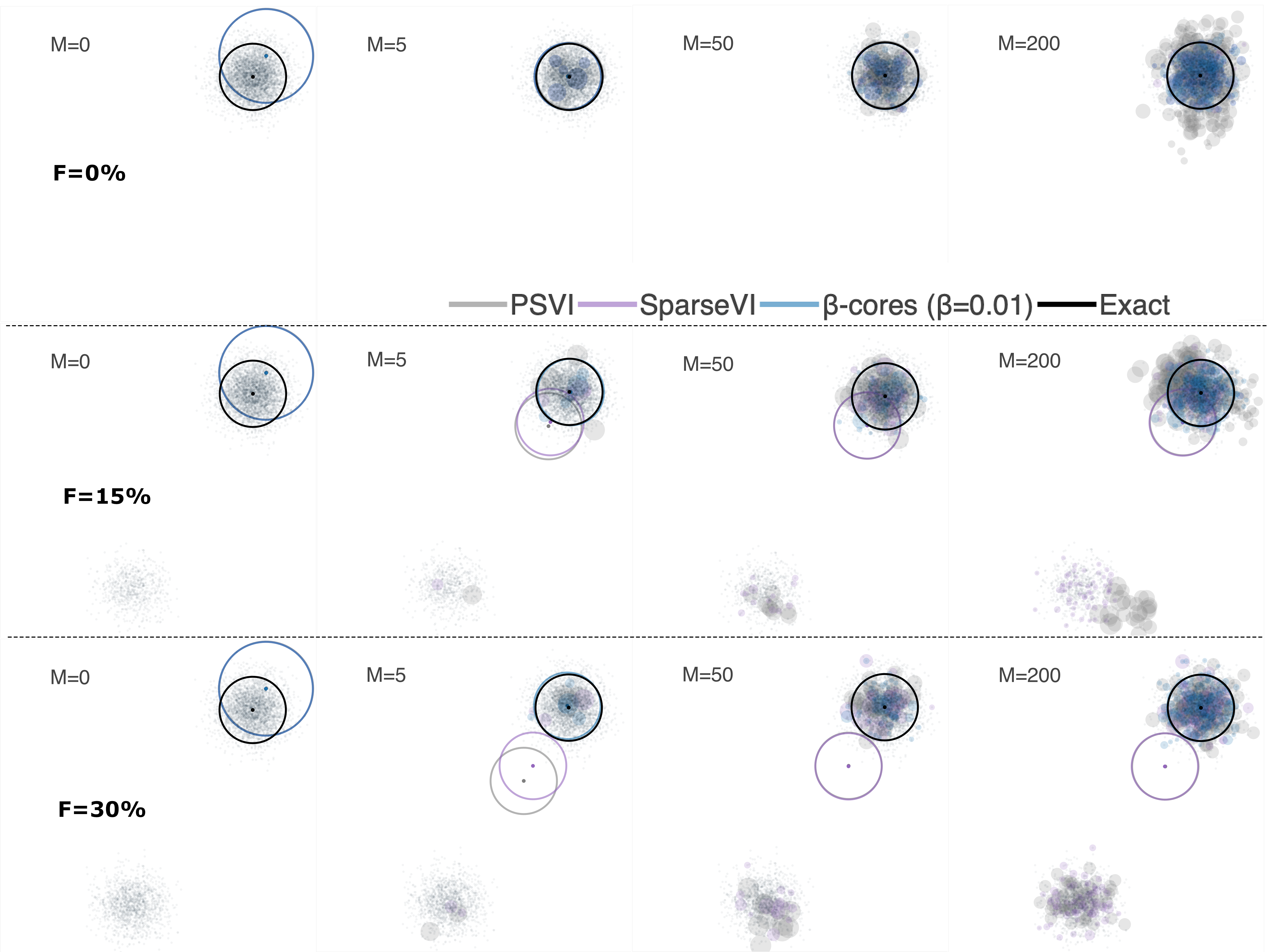


All computations involved in the coreset construction and posterior evaluation in this experiment can be performed in closed form [7]. We apply the batch scheme of Algorithm 1, sampling from the exact coreset posterior over gradient estimation. The used (-)likelihood equations are outlined in Section A.1. For all coreset methods, constructions are repeated for up to iterations, with . Notice that our setting does not imply that maximum summary size contains 200 datapoints: often over the iterations an already existing summary point may be selected again, resulting in smaller coresets.
Fig. 1(a) presents the results obtained by the different coreset methods. We stress-test their performance under varying amounts of data corruption (from top to bottom, 0%, 15%, and 30% of the datapoints get replaced by outliers). We can verify that -Cores with is on par with existing Riemannian coresets in an uncontaminated dataset. Noticeably, -Cores remains robust to high levels of structured corruption (even up to of the dataset), giving reliable posterior estimates; KL divergence plots in Fig. 1(b) reconfirm the superiority of inference via -Cores. On the other hand, in the presence of outliers, previous Riemannian coresets performance degrades quickly, offering similar posterior inference quality with random sampling. The KL divergence from the cleansed data posterior for existing summarizations and uniform sampling increases with observations failure probability, as it asymptotically converges to the Bayesian posterior computed on the corrupted dataset.
Moreover, in the case of contaminated datasets, baseline coresets are quite confident in their wrong predictive posteriors: they keep assigning the same weight to all observations and hence do not adjust their posterior uncertainty estimates, in spite of having to describe contradicting data. In contrast, -Cores discards samples from the outlying group and can confidently explain the inliers, despite the smaller effective sample size: indeed, Fig. 1(b) shows that the achieved KL divergence from the exact posterior is at same order of magnitude regardless of failure probability.
We can however notice that, for coreset sizes growing beyond 60 points—despite remaining consistently better compared to the baselines—-Cores starts to present some instability over trials in contaminated dataset instances. This effect is attributed to the small value of the hyperparameter selected for the demonstration (so that this value can successfully model the case of clean data). As a result, eventually some outliers might be allowed to enter the summary for large coreset sizes. The instability can be resolved by increasing according to the observations failure probability.
4.2 Bayesian Logistic Regression under Mislabeling and Feature Noise
In this section, we study the robustness achieved by -Cores on the problem of binary classification under unreliable measurements and labeling. We test our methods on 3 benchmark datasets with varying dimensionality (- dimensions, more details on the data are provided in Appendix B). We observe data pairs , where , , and use the Bayesian logistic regression model to describe them,
| (16) |
-likelihood terms required in our construction are computed in Section A.2.
Data corruption is simulated by generating outliers in the input and output space similarly to [20]: For corruption rate , we sample two random subsets of size from the training data. For the datapoints in the first subset, we replace the value of half of the features with Gaussian noise sampled i.i.d. from ; for the datapoints in the other subset, we flip the binary label. Over construction we use Laplace approximation [36] to efficiently draw samples from the (non-conjugate) coreset posterior, while over evaluation coreset posterior samples are obtained via NUTS [24]. We evaluate accuracy over the test set, predicting labels according to the maximum log-likelihood rule under the posterior sampling distribution. Learning rate schedule was set to , with set to 1 for SparseVI and -Cores, and 0.1 for PSVI. The values for hyperparameter and learning rates were chosen via cross-validation.


Fig. 2 illustrates that -Cores shows competitive performance with the classic Riemannian coresets in the absence of data contamination (bottom row), while it consistently achieves the best predictive accuracy in corrupted datasets (top row). On the other hand, ordinary summarization techniques, although overall outperforming random sampling for small coreset sizes, soon attain degraded predictive performance on poisoned data: by construction, via increasing coreset size, Riemannian coresets are expected to converge to the Bayesian posterior computed on the corrupted dataset. All baselines present noticeable degradation in their predictive accuracy when corruption is introduced (typically more than ), which is not the case for our method: -Cores is designed to support corrupted input and, for a well-tuned hyperparameter , maintains similar performance in the presence of outliers, while practically it can even achieve improvement (as occurring for the WebSpam data).
4.3 Neural Linear Regression on Noisy Data Batches
Here we use the coresets extension for batch summarization to efficiently train a neural linear model on selected data minibatches. Neural linear models perform Bayesian linear regression on the representation of the last layer of a deterministic neural network feature extractor [47, 43, 40]. The corresponding statistical model is as follows
| (17) |
The neural network is trained to learn an adaptive basis from datapoint pairs , which we then use to regress on , and yield uncertainty aware estimates of . More details on the model-specific formulae entering coresets construction are provided in Section A.3. Input and output related outliers are simulated as in Section 4.2, while here, for the output related outliers, gets replaced by Gaussian noise. Corruption occurs over a percentage of the total number of minibatches of the dataset, while the remaining minibatches are left uncontaminated. Each poisoned minibatch gets of its points substituted by outliers.
We evaluate -Cores, SparseVI and random sampling on two benchmark regression datasets (detailed in Appendix B). All coresets are initialized to a small batch of datapoints sampled uniformly at random from the dataset inliers. Over incremental construction, we interleave each minibatch selection and weights optimization step of the coreset with a training round for the neural network, constrained on the current coreset datapoints. Each such training round consists of minibatch gradient descent steps using the AdaGrad optimizer [16]. Our neural architecture is comprised of two fully connected hidden layers, batch normalization and ReLU activation functions. The values of coreset size at initialization, batch size added per coreset iteration, and units at each neural network hidden layer are set respectively to 20, 10 and 30 for the Housing, and 200, 100 and 100 for the Songs dataset.


Fig. 3 (bottom row) shows that -Cores are competitive with the baselines in the absence of data corruption, achieving similar predictive performance over the entire range of tested coreset sizes. Under data poisoning (top row), -Cores is the only method that offers monotonic decrease of test RMSE for increasing summary size from the beginning of the experiment. On the other hand, baselines present unreliable predictive performance for small coreset sizes: random sampling and SparseVI are both prone to including corrupted data batches, whose misguiding information gets expressed on the flexible representations learnt by the neural network, requiring a larger summary size to reach the RMSE of -Cores.
4.4 Efficient Data Acquisition from Subpopulations for Budgeted Inference
We consider the scenario where a machine learning service provider aims to fit a binary classification model to observations coming from multiple subpopulations of data contributors. The provider aims to maximize the predictive accuracy of the model, while adhering to a budget on the total number of subpopulations from which data can be used over inference. Budgeted inference can be motivated by several practical requirements: First, restricting the total number of datapoints used over learning to a smaller informative subset aids scalability—which is the primary motivation for coresets. Moreover, taking decisions at the subpopulations level regarding which groups of datapoints are useful for the task, without the need to inspect datapoints individually, reduces the privacy loss incurred over the data selection stage, and can be integrated in machine learning pipelines that follow formal hierarchical privacy schemes. Finally, subpopulations valuation can guide costly experimental procedures, via inducing knowledge regarding which group combinations are most beneficial in summarizing the entire population of interest [40, 50], and hence should be prioritised over data collection.
In this study we use a subset of more than datapoints from the HospitalReadmissions dataset (for further details see Appendix B). Using combinations of age, race and gender information of data contributors, we form a total of subpopulations within the training dataset. Data contamination is simulated identically to the experiment of Section 4.2, while now we also consider the case of varying levels of contamination across the subpopulations. In particular, we form groups of roughly equal size where and of the datapoints get replaced by outliers—this results in getting a dataset with approximately of its full set of datapoints corresponding to outliers.


We evaluate the predictive accuracy achieved by doing inference on the data subset obtained after running iterations of the -Cores extension for groups (which gives a maximum of selected groups). We compare against (i) a random sampler, and (ii) a baseline which ranks all groups according to their Shapley value and selects the groups with the highest values. Shapley value is a concept originating in cooperative game theory [45], which has recently found applications in data valuation and outliers detection [21]. In the context of our experiment, it quantifies what is the marginal contribution of each group to the predictive accuracy of the model at all possible group coalitions that can be formed. As this quantity is notoriously expensive to be computed in large datasets, we use a Monte Carlo estimator which samples possible permutations of groups and for each permutation it computes marginals for coalitions formed by the first groups.§§ § The latter truncation is supported by the observation that marginal contributions to the predictive accuracy are diminishing as the dataset size increases.
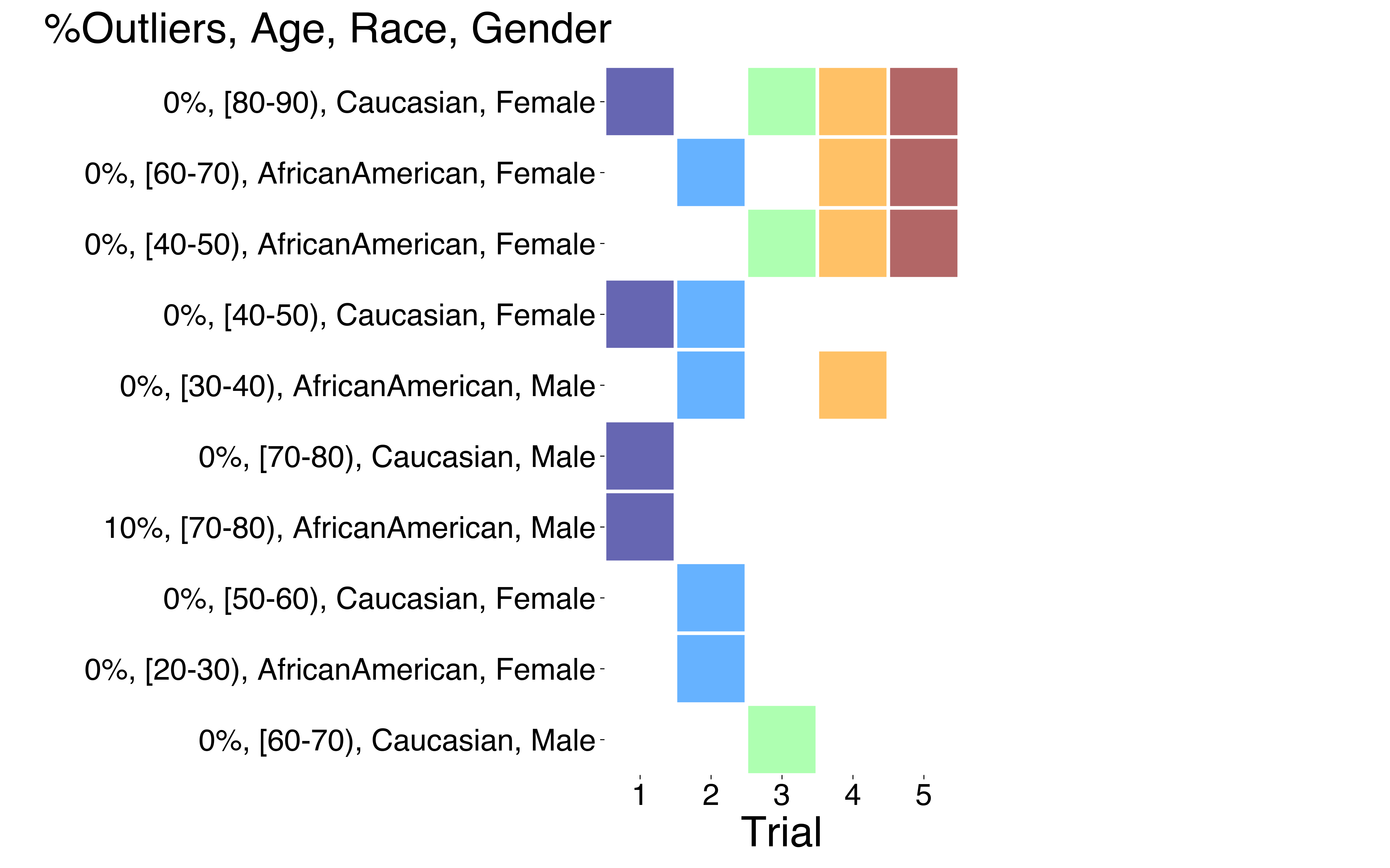
As illustrated in Fig. 4, -Cores with offers the best solution to our problem, and is able to reach predictive accuracy exceeding by fitting a coreset on no more than groups. Fig. 5 displays the demographic information of selected groups. We can notice that subpopulations of female and older patients are more informative for the classification task, while Caucasian and African-American groups are preferred to smaller racial minorities. Importantly, -Cores is able to distill clean from contaminated groups. For used value we can see than over the set of trials only one group with outliers level of is allowed to enter a summary, which already contains uncontaminated groups.
Shapley values based ranking treats outliers better than random sampling: As outliers are expected to have negative marginal contribution to predictive accuracy, their Shapley rank is generally lower compared to clean data groups. On the other hand, Shapley computation is much slower than random sampling and -Cores, specific to the evaluation metric of interest, while Shapley values are not designed to find data-efficient combinations of groups, hence this baseline can still return redundancy in the selected data subset.
5 Conclusion & further directions
In this work, we proposed a general purpose framework for yielding contamination-robust summarizations of massive scale datasets for inference. Relying on recent advances in Bayesian coresets and robustified inference under the -divergence, we developed a greedy black-box construction that efficiently shrinks big data via keeping informative datapoints, while simultaneously rejecting outliers. Finally, we presented experiments involving various statistical models, and simulated and real-world datasets, demonstrating that our methodology outperforms existing techniques in scenarios of structured and unstructured data corruption.
Our future work will be concerned with considering stronger adversarial settings where summaries are initialized to data subsets that already contain outliers. Further directions also include automating the tuning of the robustness hyperparameter , as well as applying our techniques to more complicated statistical models, including ones with structured likelihood functions (e.g. time-series and temporal point processes).
6 Acknowledgements
This work is partially supported by Nokia Bell Labs through their donation for the Centre of Mobile, Wearable Systems and Augmented Intelligence to the University of Cambridge. DM also gratefully acknowledges the support received from Lundgren Fund and Darwin College Cambridge. We thank Trevor Campbell for helpful discussions on Bayesian coresets.
Appendix A Models
In this section we present the derivations of -likelihood terms Eqs. 6 and 7 required over the -Cores constructions for the statistical models of our experiments.
A.1 Gaussian likelihoods
For the -likelihood terms of a multivariate normal distribution, we have
| (18) |
and, by simple calculus (see also [44]),
| (19) |
Hence
| (20) | ||||
| (21) | ||||
| (22) |
A.2 Logistic regression likelihoods
Log-likelihood terms of individual datapoints are given as follows
| (23) |
Substituting to Eq. 7, for the -likelihood terms we get
| (24) | ||||
| (25) |
A.3 Neural linear regression likelihoods and predictive posterior
Recall that in the neural linear regression model, , . Then the Gaussian log-likelihoods corresponding to individual observations (after dropping normalization constants), are written as
| (26) |
Assuming a prior , the coreset posterior can be computed in closed form as follows
| (27) |
where
| (28) | ||||
| (29) |
By substitution to Eq. 7, the -likelihood terms for our adaptive basis linear regression are written as
| (30) |
Let be the output of the coreset applied on a dataset . Hence, in regression problems, the predictive posterior on a test data pair via a coreset is approximated as follows
| (31) | ||||
| (32) |
In the neural linear experiment, the predictive posterior is a Gaussian given by the following formula
| (33) |
Appendix B Datasets Details
The benchmark datasets used in logistic regression (including group selection) and neural linear regression experiments are detailed in Tables 1 and 2 respectively.¶¶ ¶ The original versions of all used datasets can be accessed by following the corresponding hyperlinks in the Tables appearing in the electronic version of the paper., and include:
- •
a dataset used to predict whether a citizen’s income exceeds per year extracted from USA 1994 census data (Adult),
- •
a dataset containing webpages features and a label categorizing them as phishing or not (Phishing),
- •
a corpus of webpages crawled from links found in spam emails (WebSpam),
- •
a set of hospitalization records for binary prediction of readmission pertaining to diabetes patients (HospitalReadmissions),
- •
a set of various features from homes in the suburbs of Boston, Massachussets used to model housing price (Housing), and
- •
a dataset used to predict the release year of songs from associated audio features (Songs).
For Adult, Phishing and HospitalReadmissions we fit our statistical models on the first 10 principal components of the datasets, while all logistic regression benchmark datasets are evaluated on balanced subsets of the test data between the two classes (see Table 1).
References
- [1] E. Angelino, M. J. Johnson, and R. P. Adams. Patterns of scalable Bayesian inference. Found. Trends Mach. Learn., 2016.
- [2] M. Barreno, B. Nelson, A. D. Joseph, and J. D. Tygar. The security of machine learning. Machine Learning, 2010.
- [3] A. Basu, I. R. Harris, N. L. Hjort, and M. C. Jones. Robust and efficient estimation by minimising a density power divergence. Biometrika, 85(3):549–559, 1998.
- [4] J. O. Berger, E. Moreno, L. R. Pericchi, M. J. Bayarri, J. M. Bernardo, J. A. Cano, J. De la Horra, J. Martín, D. Ríos Insua, B. Betrò, et al. An overview of robust Bayesian analysis. Test, 3(1):5–124, 1994.
- [5] K. Bhatia, Y.-A. Ma, A. D. Dragan, P. L. Bartlett, and M. I. Jordan. Bayesian Robustness: A Nonasymptotic Viewpoint. arXiv preprint, 2019.
- [6] B. Biggio, B. Nelson, and P. Laskov. Poisoning attacks against support vector machines. In Proceedings of the 29th International Coference on International Conference on Machine Learning, 2012.
- [7] T. Campbell and B. Beronov. Sparse variational inference: Bayesian coresets from scratch. In Advances in Neural Information Processing Systems, 2019.
- [8] T. Campbell and T. Broderick. Automated scalable Bayesian inference via Hilbert coresets. Journal of Machine Learning Research, 20(15), 2019.
- [9] M. Chen, C. Gao, and Z. Ren. Robust covariance and scatter matrix estimation under Huber’s contamination model. The Annals of Statistics, 46(5):1932–1960, 2018.
- [10] A. Cichocki and S. Amari. Families of alpha- beta- and gamma- divergences: Flexible and robust measures of similarities. Entropy, 12(6):1532–1568, 2010.
- [11] A. P. Dawid, M. Musio, and L. Ventura. Minimum scoring rule inference. Scandinavian Journal of Statistics, 43(1):123–138, 2016.
- [12] B. de Finetti. The bayesian approach to the rejection of outliers. In Proceedings of the fourth Berkeley Symposium on Probability and Statistics, 1961.
- [13] I. Diakonikolas, G. Kamath, D. Kane, J. Li, J. Steinhardt, and A. Stewart. Sever: A robust meta-algorithm for stochastic optimization. In Proceedings of the 36th International Conference on Machine Learning, 2019.
- [14] C. Dickens, E. Meissner, P. G. Moreno, and T. Diethe. Interpretable anomaly detection with Mondrian Pólya forests on data streams. arXiv preprint, 2020.
- [15] D. Dua and C. Graff. UCI machine learning repository, 2017.
- [16] J. Duchi, E. Hazan, and Y. Singer. Adaptive subgradient methods for online learning and stochastic optimization. Journal of Machine Learning Research, 12(61):2121–2159, 2011.
- [17] S. Eguchi and Y. Kano. Robustifying maximum likelihood estimation. Tokyo Institute of Statistical Mathematics, Tokyo, Japan, Tech. Rep, 2001.
- [18] B. Frénay and M. Verleysen. Classification in the presence of label noise: a survey. IEEE transactions on neural networks and learning systems, 25(5), 2013.
- [19] H. Fujisawa and S. Eguchi. Robust parameter estimation with a small bias against heavy contamination. J. Multivar. Anal., pages 2053–2081, 2008.
- [20] F. Futami, I. Sato, and M. Sugiyama. Variational inference based on robust divergences. In Proceedings of the Twenty-First International Conference on Artificial Intelligence and Statistics, 2018.
- [21] A. Ghorbani and J. Zou. Data shapley: Equitable valuation of data for machine learning. In Proceedings of the 36th International Conference on Machine Learning, 2019.
- [22] A. Ghosh and A. Basu. Robust Bayes estimation using the density power divergence. Annals of the Institute of Statistical Mathematics, 68(2):413–437, 2016.
- [23] M. D. Hoffman, D. M. Blei, C. Wang, and J. Paisley. Stochastic variational inference. Journal of Machine Learning Research, 14:1303–1347, 2013.
- [24] M. D. Hoffman and A. Gelman. The No-U-Turn sampler: Adaptively setting path lengths in Hamiltonian Monte Carlo. Journal of Machine Learning Research, 15(1):1593–1623, 2014.
- [25] P. J. Huber. Robust estimation of a location parameter. In Breakthroughs in statistics, pages 492–518. Springer, 1992.
- [26] P. J. Huber and E. M. Ronchetti. Robust statistics; 2nd ed. Wiley Series in Probability and Statistics. Wiley, Hoboken, NJ, 2009.
- [27] J. Huggins, T. Campbell, and T. Broderick. Coresets for scalable Bayesian logistic regression. In Advances in Neural Information Processing Systems, 2016.
- [28] J. Jewson, J. Q. Smith, and C. Holmes. Principles of bayesian inference using general divergence criteria. Entropy, 20(6):442, 2018.
- [29] D. R. Karger, S. Oh, and D. Shah. Iterative learning for reliable crowdsourcing systems. In Advances in neural information processing systems, 2011.
- [30] J. Knoblauch, J. E. Jewson, and T. Damoulas. Doubly robust Bayesian inference for non-stationary streaming data with -divergences. In Advances in Neural Information Processing Systems 31, 2018.
- [31] P. W. Koh and P. Liang. Understanding black-box predictions via influence functions. In Proceedings of the 34th International Conference on Machine Learning, 2017.
- [32] R. Kohavi. Scaling up the accuracy of naive-Bayes classifiers: A decision-tree hybrid. In KDD, 1996.
- [33] D. D. Lewis, Y. Yang, T. G. Rose, and F. Li. RCV1: A new benchmark collection for text categorization research. J. Mach. Learn. Res., 5:361–397, Dec. 2004.
- [34] B. Li, Y. Wang, A. Singh, and Y. Vorobeychik. Data poisoning attacks on factorization-based collaborative filtering. In Advances in neural information processing systems, 2016.
- [35] Q. Liu, J. Peng, and A. T. Ihler. Variational inference for crowdsourcing. In Advances in Neural Information Processing Systems 25, 2012.
- [36] D. J. C. MacKay. Information Theory, Inference, and Learning Algorithms. Cambridge University Press, 2003.
- [37] D. Manousakas, Z. D. Xu, C. Mascolo, and T. Campbell. Bayesian pseudocoresets. preprint, 2020.
- [38] J. W. Miller and D. B. Dunson. Robust Bayesian inference via coarsening. Journal of the American Statistical Association, 114(527), 2019.
- [39] P. Paschou, J. Lewis, A. Javed, and P. Drineas. Ancestry informative markers for fine-scale individual assignment to worldwide populations. Journal of Medical Genetics, 2010.
- [40] R. Pinsler, J. Gordon, E. Nalisnick, and J. M. Hernández-Lobato. Bayesian batch active learning as sparse subset approximation. In Advances in Neural Information Processing Systems, 2019.
- [41] V. C. Raykar, S. Yu, L. H. Zhao, G. H. Valadez, C. Florin, L. Bogoni, and L. Moy. Learning from crowds. Journal of Machine Learning Research, 11(4), 2010.
- [42] D. Ríos Insua and F. Ruggeri. Robust Bayesian Analysis, volume 152. Springer Science & Business Media, 2012.
- [43] C. Riquelme, G. Tucker, and J. Snoek. Deep Bayesian bandits showdown: An empirical comparison of Bayesian deep networks for Thompson sampling. In 6th International Conference on Learning Representations, 2018.
- [44] W. Samek, D. Blythe, K.-R. Müller, and M. Kawanabe. Robust spatial filtering with beta divergence. In Advances in Neural Information Processing Systems, 2013.
- [45] L. S. Shapley. A value for n-person games. Contributions to the Theory of Games, 2(28), 1953.
- [46] V. S. Sheng, F. Provost, and P. G. Ipeirotis. Get another label? improving data quality and data mining using multiple, noisy labelers. In Proceedings of the 14th ACM SIGKDD International Conference on Knowledge Discovery and Data Mining, 2008.
- [47] J. Snoek, O. Rippel, K. Swersky, R. Kiros, N. Satish, N. Sundaram, M. Patwary, M. Prabhat, and R. Adams. Scalable bayesian optimization using deep neural networks. In Proceedings of the 32nd International Conference on Machine Learning, 2015.
- [48] J. Steinhardt, P. W. W. Koh, and P. S. Liang. Certified defenses for data poisoning attacks. In Advances in neural information processing systems, 2017.
- [49] B. Strack, J. P. DeShazo, C. Gennings, J. L. Olmo, S. Ventura, K. J. Cios, and J. N. Clore. Impact of HbA1c measurement on hospital readmission rates: analysis of 70,000 clinical database patient records. BioMed research international, 2014.
- [50] S. Vahidian, B. Mirzasoleiman, and A. Cloninger. Coresets for estimating means and mean square error with limited greedy samples. In Proceedings of the 36th Conference on Uncertainty in Artificial Intelligence, 2020.
- [51] M. J. Wainwright and M. I. Jordan. Graphical models, exponential families, and variational inference. Found. Trends Mach. Learn., 1(1-2):1–305, Jan. 2008.
- [52] C. Wang and D. M. Blei. A general method for robust Bayesian modeling. Bayesian Analysis, 2018.
- [53] D. Wang, D. Irani, and C. Pu. Evolutionary study of web spam: Webb Spam Corpus 2011 versus Webb Spam Corpus 2006. In 8th International Conference on Collaborative Computing: Networking, Applications and Worksharing, 2012.
- [54] Y. Wang, A. Kucukelbir, and D. M. Blei. Robust probabilistic modeling with Bayesian data reweighting. In Proceedings of the 34th International Conference on Machine Learning, 2017.
- [55] X. Wei and S. Minsker. Estimation of the covariance structure of heavy-tailed distributions. In Advances in Neural Information Processing Systems, 2017.
- [56] M. Welling and Y. W. Teh. Bayesian learning via stochastic gradient Langevin dynamics. In Proceedings of the 28th international conference on machine learning, 2011.
- [57] J. Whitehill, T.-f. Wu, J. Bergsma, J. R. Movellan, and P. L. Ruvolo. Whose vote should count more: Optimal integration of labels from labelers of unknown expertise. In Advances in neural information processing systems, 2009.
- [58] A. Zellner. Optimal information processing and bayes’s theorem. The American Statistician, 42(4):278–280, 1988.
- [59] Y. Zhang, X. Chen, D. Zhou, and M. I. Jordan. Spectral methods meet EM: A provably optimal algorithm for crowdsourcing. The Journal of Machine Learning Research, 17(1):3537–3580, 2016.
- [60] V. W. Zheng, S. J. Pan, Q. Yang, and J. J. Pan. Transferring multi-device localization models using latent multi-task learning. In AAAI, 2008.
- [61] H. Zhuang, A. Parameswaran, D. Roth, and J. Han. Debiasing crowdsourced batches. In Proceedings of the 21th ACM SIGKDD International Conference on Knowledge Discovery and Data Mining, 2015.