Asymptotically flat hairy black holes in massive bigravity
Abstract
We study asymptotically flat black holes with massive graviton hair within the ghost-free bigravity theory. There have been contradictory statements in the literature about their existence – such solutions were reported some time ago, but later a different group claimed the Schwarzschild solution to be the only asymptotically flat black hole in the theory. As a result, the controversy emerged. We have analyzed the issue ourselves and have been able to construct such solutions within a carefully designed numerical scheme. We find that for given parameter values there can be one or two asymptotically flat hairy black hole solutions in addition to the Schwarzschild solution. We analyze their perturbative stability and find that they can be stable or unstable, depending on the parameter values. The masses of stable hairy black holes that would be physically relevant range form stellar values up to values typical for supermassive black holes. One of their two metrics is extremely close to Schwarzschild, while all their “hair” is hidden in the second metric that is not coupled to matter and not directly seen. If the massive bigravity theory indeed describes physics, the hair of such black holes should manifest themselves in violent processes like black hole mergers and should be visible in the structure of the signals detected by LIGO/VIRGO.
I INTRODUCTION
Theories with massive gravitons provide a natural modification of the general relativity (GR) in the infrared regime and can be used to explain the current acceleration of our Universe 1538-3881-116-3-1009; 0004-637X-517-2-565. Such theories have a long history pioneered by the work of Fierz and Pauli Fierz:1939ix and marked by subsequent discoveries of many interesting features, such as the vDVZ discontinuity vanDam:1970vg; Zakharov:1970cc, the Vainshtein mechanism Vainshtein:1972sx, the Boulware-Deser ghost Boulware:1973my, culminating in the discovery of the ghost-free massive gravity deRham:2010kj and ghost-free bigravity Hassan2012 theories.
The ghost-free bigravity theory is the most interesting physically. It contains two dynamical metrics, usually called and , describing together two gravitons, one of which is massive and the other is massless. The theory admits self-accelerating cosmological solutions Volkov:2011an; vonStrauss:2011mq; Comelli:2011zm whose properties can agree with the observations Akrami:2015qga; Mortsell:2015exa; Aoki:2015xqa; Luben:2018ekw; Hogas:2019ywm, with the term mimicked by the graviton mass. The theory also admits solutions describing black holes Volkov2012, wormholes Sushkov:2015fma, and other interesting solutions (see Volkov:2013roa for a review). In what follows we shall be discussing black holes.
The bigravity black holes can be either “bald” or “hairy”. The bald black holes are described by the known GR metrics. Such solutions were first discovered long ago Isham:1977rj; Gurses:1979qb; Gurses:1981an within the old bigravity theory inspired by physics of strong interactions Isham:1971gm. In the simplest case, their two metrics are both Schwarzschild-(anti-)de Sitter and can be conveniently represented in the Eddington-Finkelstein coordinates as Babichev:2014oua; Volkov:2014ooa
| (1.1) |
with and , where values of constants are fixed by the field equations. Passing to the Schwarzschild coordinates, one can diagonalize one of the two metrics, but not both of them simultaneously. Such solutions have been much studied Berezhiani:2008nr, they exist also within the ghost-free bigravity Comelli:2011wq, and they admit the charged Babichev:2014fka and spinning Babichev:2014tfa generalizations. These solutions also admit the massive gravity limit where hence the f metric is flat while the g metric remains nontrivial, and this yields all possible static black holes in the ghost-free massive gravity theory (it seems there can be also time-dependent black holes in this theory Rosen:2018lki).
Next, it was noticed in Volkov2012 that if the parameters of the potential are suitably adjusted, then the ghost-free bigravity reduces to the vacuum GR when the two metrics coincide, . Therefore, all vacuum black holes, as for example the Schwarzschild solution (to be called bald to distinguish it from the “hairy Schwarzschild” to be described below),
| (1.2) |
or its spinning generalization can be imbedded into the ghost-free bigravity. A term can be included by assuming the two metrics to be proportional to each other Volkov2012; Volkov:2013roa; Volkov:2014ooa. Such solutions are different from solutions of type (1.1), for example they do not admit the massive gravity limit. In addition, the solution (1.1) is linearly stable Babichev:2015zub, whereas (1.2) is unstable (for a small ) with respect to fluctuations which do not respect the condition Babichev:2013una.
These facts essentially exhaust the available knowledge of the bald black holes in the bigravity theory. At the same time, more general hairy black holes not described by the classical GR metrics can exist as well. The first example of hairy black holes in physics was found long ago Volkov:1989fi, followed by many other examples (see Volkov:1998cc; Volkov:2016ehx for a review), so that nowadays hairy black holes are considered as something usual. One may therefore wonder if they exist in the ghost-free bigravity theory as well.
A systematic analysis of hairy black holes in the ghost-free massive bigravity has been carried out for the first time by one of the authors Volkov2012, but none of the solutions found were asymptotically flat. In that analysis both metrics were assumed to be static and spherically symmetric. If they are not simultaneously diagonal, then the most general solution is given by (1.1). If they are simultaneously diagonal, then one of the solutions is given by (1.2), but other more general black hole solutions exist as well.
Such solutions possess an event horizon – a hypersurface that is null simultaneously with respect to and . Therefore, both metrics share the horizon Deffayet:2011rh; Banados:2011hk, but its radius measured by can be different from the radius measured by . One can set to unit value via rescaling the system (rescaling at the same time the graviton mass), but the ratio is scale invariant. Choosing a value of completely determines the boundary conditions at the horizon, which allows one to integrate the equations starting from the horizon toward large values of the radial coordinate . As a result, the set of all black hole solutions can be labeled by just one parameter , and integrating the equations for different values of gives all possible black holes.
Choosing yields the Schwarzschild solution (1.2). For one finds more general black holes supporting a massive graviton “hair” outside the horizon, but in the asymptotic region their two geometries do not become flat Volkov2012. The latter property is generic, and trying different values of always gives either solutions with a curvature singularity somewhere outside the horizon, or solutions which exist for all values of but show nonflat asymptotics.
At the same time, these facts do not completely exclude a possibility of some other asymptotically flat black hole solutions different from (1.2), which would correspond to some special values of different from . However, even if they exist, one does not find such solutions by a brute force via trying many different values of , and the reason is the following. The field equations reduce to three coupled first order ordinary differential equations (ODEs) Volkov2012, whose local at large solution has schematically the following structure when it is linearized around flat space ( being integration constants):
| (1.3) |
Here is the dimensionless radial coordinate, with m and r being the graviton mass and dimensionful radial coordinate (we assume the graviton mass to have the dimension of inverse length, so that this is rather the inverse Compton wavelength ). The Newtonian mode in (1.3) arises due to the massless graviton present in the theory, while the decaying mode and the growing mode are due to the massive graviton. Now, when integrating from the horizon, the growing mode will be inevitably present in the numerical solution at large and will drive the solution away from flat space. This is why one does not find asymptotically flat solutions in this way.
To get them, one should suppress the growing mode by setting , hence the local solutions at large will comprise a two-parameter set labeled by and . The next step is to numerically extend this local solution toward small , extending at the same time the local solution at the horizon labeled by toward large , until the two solutions meet at some intermediate point. For these solutions to agree, three (the number of the ODEs) matching conditions should be satisfied via adjusting the three parameters . In practice, this can be done within the numerical multiple-shooting method Press:2007:NRE:1403886. Once are adjusted, this yields global asymptotically flat solutions.
The difficulty, however, is that the numerical scheme requires some input values for , which should be close to the “true values”, otherwise the iterations do not converge. It was a priory unclear how to choose these input values, whereas choosing them randomly does not give the convergence. Some additional information was needed to properly choose these input values, but at the time of writing the article Volkov2012 such information was not available. As a result, the conclusion of that work was that asymptotically flat hairy black holes may exist, but they should be parametrically isolated form the Schwarzschild solution (1.2).
It is interesting that by adding an extra matter source to obtain not a black hole but a regular object like a star, asymptotically flat solutions can be easily constructed, as was shown first in Volkov2012 and later in Enander:2015kda; Aoki:2016eov. The black hole case is more difficult.
Fortunately, the additional information was later obtained within the analysis of perturbations of the Schwarzschild solution (1.2) Babichev:2013una; Brito:2013wya. Denoting the Schwarzschild metric, the two perturbed metrics are and . Linearizing the field equations with respect to and , one finds that perturbations grow in time and hence the background Schwarzschild black hole is unstable if . On the other hand, for the perturbations are bounded in time so that the background is stable Babichev:2013una. Curiously, the mathematical structure of the perturbation equations is identical Babichev:2013una to that previously discovered by Gregory and Laflamm (GL) in their analysis of black strings in GR Gregory:1993vy. We shall therefore refer to the Schwarzschild solution with as GL point.
This change of stability at the GL point suggests that for close to there could be two different asymptotically flat solutions: the Schwarzschild solution (1.2) and also some other solution which can be approximated by the zero perturbation mode that exists at the GL point. This new solution is different from Schwarzschild although close to it, hence it describes an asymptotically flat hairy black hole. To get this solution within the numerical scheme outlined above, one should choose the input parameters to be close the GL point, , , , , and it is this essential piece of information that was missing when writing Ref.Volkov2012. As soon as the solution is obtained, one can change the value of iteratively, thus obtaining “fully fledged” hairy black holes which may deviate considerably from the parent Schwarzschild solution.
Remarkably, this program was accomplished by the Portuguese group Brito:2013xaa via explicitly constructing asymptotically flat hairy black holes in the theory in the region below the GL point, for . However, some time later spherically symmetric bigravity solutions were analyzed by the Swedish group Torsello:2017cmz, and it was claimed that the Schwarzschild solution (1.2) represents the unique asymptotically flat black hole in the theory. As a result, a controversy emerged and it was unclear if asymptotically flat hairy black holes exist or not.
We have therefore reconsidered the issue ourselves and below are our results. In brief, we were able to construct asymptotically flat hairy black holes in the theory, thereby confirming the finding of Brito:2013xaa. We apply a very carefully designed numerical scheme to exclude any ambiguities and to take into account the arguments of Torsello:2017cmz. In fact, these arguments correctly point to some drawbacks of the numerical analysis commonly present in many publications. From the mathematical viewpoint, one has to solve a nonlinear boundary value problem where the boundaries are singular points of the differential equations (horizon and infinity). Since it is difficult to approach such points numerically, various approximations are used in practice, which may give reasonable results in some cases but inevitably increase the numerical errors and lead to a numerical instability. Only very rarely does one find in the literature a correct treatment of the problem (apart from the relaxation approach), as for example in Breitenlohner:1991aa; BFM; Breitenlohner:1993es. We therefore pay special attention to the details of our numerical scheme and describe them in a very explicit way. From the methodological viewpoint, our paper gives an example of how one should properly tackle a nonlinear boundary value problem with singular endpoints.
We cross-check our results with two different numerical codes written independently by two of us. Our results strongly suggest that the hairy solutions exist and are indeed asymptotically flat and regular. We discover many new features of these solutions, for example we obtain hairy black holes also above the GL point for , and we study for the first time the perturbative stability of the solutions. We were able to identify regions in the parameter space which correspond to stable solutions, and we determined subsets of these regions which agree with the constraints imposed by the cosmological observations. We find that the viable hairy black holes should be described by the g metric that is very close to Schwarzschild, but their f metric is different. Therefore, if the bigravity theory indeed describes physics, the astrophysical black holes should hide the hair in their f-metric. We find masses of such black holes to range from to .
We have also attentively considered the arguments of Ref. Torsello:2017cmz. In brief, this work seems to agree that the hairy solutions exist but judges them physically unacceptable. We analyze the arguments and we think some of them are interesting and should be taken into consideration, but none of them is decisive, so that they should rather be viewed as a conjecture. To understand its origin, we notice that the numerical procedure adopted in that work is not suitable for suppressing the growing at infinity mode, which generates artificial numerical singularities. This must be the reason why the solutions were judged unacceptable in that work. However, no singularities appear within the properly chosen numerical scheme, and we specially adapt our scheme to be able to cope with the arguments of Torsello:2017cmz. We shall postpone a more detailed discussion of Ref. Torsello:2017cmz until the end of this text to be able to make a comparison with our results.
The rest of the text is organized as follows. In Sec. II we introduce the massive bigravity theory of Hassan and Rosen Hassan2012. The field equations, their reduction to the static and spherically symmetric sector, and the simplest solutions are described in Sec. III–V. In Sec. VI,VII we describe in detail our analysis of boundary conditions at the horizon and at infinity, and then summarize in Sec. VIII the structure of our numerical procedure. In Sec. IX we show our solutions for asymptotically flat hairy black holes and also describe the duality relation yielding the solutions above the GL point. After that, we discuss in Sec. X the perturbations of the hairy backgrounds and the analysis of the negative perturbation modes. Our discussion culminates in Sec. XI where we describe various limits and identify regions in the parameter space where the solutions exist and where they are stable. In Sec. XII we give a brief summary of our results and discuss the arguments of Ref.Torsello:2017cmz. The two appendixes contain the description of the desingularization of the equations at the horizon, as well as the complete set of the field equations in the time-dependent case.
II THE GHOST-FREE BIGRAVITY
The theory is defined on a four-dimensional spacetime manifold endowed with two Lorentzian metrics and with the signature . The action is Hassan2012
| (2.1) |
where and are the gravitational couplings, is a parameter with the same dimension, and is a mass parameter. The interaction between the two metrics is expressed by a scalar function of the tensor (the hat denotes matrices)
| (2.2) |
Here the matrix square root is understood in the sense that , which can be written in components as
| (2.3) |
If () are the eigenvalues of then the interaction potential is
| (2.4) |
where are dimensionless parameters while are defined by the relations
Here and . The two metrics actually enter the action in a completely symmetric way, since the action is invariant under
| (2.5) |
The action is also invariant under rescalings , , and this allows one to impose, without any loss of generality, the normalization condition . Varying the action with respect to the two metrics gives two sets of Einstein equations,
| (2.6) |
where and , and the normalization of implies that . The source terms in (2.6) are obtained by varying the interaction potential ,
| (2.7) |
where is the inverse of and
| (2.8) | |||||
There is an identity relation following from the diffeomorphism invariance of the interaction term in the action,
| (2.9) |
where and are the covariant derivatives with respect to gμν and fμν.
Equations (2.6) describe two interacting gravitons, one massive and one massless. This can be easily seen in the flat space limit. Setting (the Minkowski metric), Eqs.(2.6) reduce to
| (2.10) |
with . Therefore, the flat space will be a solution if only the parameters fulfil the conditions . Assuming this to be the case, let us set and where the deviations and are small. Linearizing the equations (2.6) with respect to the deviations yields
| (2.11) | |||
| (2.12) |
where denotes the linear part of the Einstein operator, and where and with . The equations are the linearized Einstein equations describing a massless graviton with two dynamical polarizations. The field fulfills the Fierz-Pauli equations for massive gravitons with five polarizations and with the mass
| (2.13) |
Therefore, one will have if
| (2.14) |
This condition can be solved together with the conditions implied by (2.10) to express the five in terms of two independent parameters, sometimes called and ,
| (2.15) |
At the same time, the theory has exactly 7 propagating degrees of freedom also away from the flat space limit and for arbitrary (see Hassan:2011ea; Alexandrov:2013rxa; Soloviev:2020zht for its Hamiltonian formulation).
Let us finally pass from the dimensionful spacetime coordinates to the dimensionless ones,
| (2.16) |
This is equivalent to the conformal rescaling of the metrics,
| (2.17) |
after which the field equations (2.6) reduce to
| (2.18) |
where and are still given by (2.7),(2.8) with . The Bianchi identities for these equations imply that
| (2.19) |
which is consistent with (2.9). All fields and coordinates are now dimensionless and no trace of the mass parameter m is left in the equations. However, one has to remember that the unity of length corresponds to the dimensionful , which is the physical length scale.
In what follows we shall be analyzing equations (2.18) without making any assumptions about values of , and . However, when integrating the equations numerically, we shall assume that and choose according to (2.15). Therefore, our solutions depend on three parameters of the theory, and , where
| (2.20) |
We shall assume in what follows that if the theory is extended to include an extra matter variables denoted by , then the action (2.1) becomes , so that the matter couples only to the g metric. The g-geometry is therefore physically measurable as test particles follow its geodesics. The f-geometry is not directly coupled to matter, hence it cannot be directly seen and remains hidden.
III SPHERICAL SYMMETRY
Let us introduce coordinates and choose both metrics to be static, spherically symmetric, and diagonal,
| (3.1) |
where while are functions of the radial coordinate . In fact, this is not the most general form of the spherically symmetric fields, since one could also include the off-diagonal metric element as shown by Eq.(B.31) in Appendix APPENDIX B: FIELD EQUATIONS WITH TIME DEPENDENCE. However, in the static case this would imply that (1.1) is the only possible solution Volkov2012 (the situation changes in the time-dependent case). Therefore, we choose the static metrics to be both diagonal, which leads to nontrivial solutions.
The tensor in (2.2) then reads
| (3.2) |
and one obtains from (2.7)
| (3.3) |
where
| (3.4) |
Here and
| (3.5) |
The independent field equations are
| (3.6) |
plus the conservation condition which has only one nontrivial component,
| (3.7) |
where the prime denotes differentiation with respect to . The conservation condition for the second energy-momentum tensor also has only one nontrivial component,
| (3.8) |
but this follows from (3.7) due to the identity relation (2.9). As a result, there are 5 independent equations in (III), (3.7), which is enough to determine the 6 field amplitudes , because the freedom of reparametrization of the radial coordinate allows one to fix one of the amplitudes.
IV FIELD EQUATIONS
Let us introduce new functions
| (4.1) |
in terms of which the two metrics read
| (4.2) |
The advantage of this parametrization is that the second derivatives disappear from the Einstein tensor and the four Einstein equations (III) become
| (4.3) | |||||
| (4.4) | |||||
| (4.5) | |||||
| (4.6) |
The conservation condition (3.7) reads
| (4.7) |
and using Eqs.(4.5) and (4.6), this reduces to
| (4.8) |
where
| (4.9) | |||||
with
| (4.10) |
The conservation condition (3.8) becomes
| (4.11) |
The two conditions (4.8) and (4.11) will be fulfilled if , in which case both metrics are degenerate. If the metrics are not degenerate, then conditions (4.8) and (4.11) reduce to the algebraic constraint
| (4.12) |
This constraint can be resolved with respect to to give
| (4.13) |
where is the (negative) ratio of the coefficients in front of and in (4.9).
As a result, we obtain four differential equations (4.3)–(4.6) plus one algebraic constraint (4.12). The same equations can be obtained by inserting the metrics (IV) directly to the action (2.1), which gives
| (4.14) |
where, dropping a total derivative,
| (4.15) | |||||
Varying with respect to gives Eqs.(4.3)–(4.6), while varying it with respect to reproduces conditions (4.8) and (4.11). The equations and the Lagrangian are invariant under the interchange symmetry (2.5), which now reads
| (4.16) |
Equations (4.3)–(4.6) contain and which are not yet known. One of these two amplitudes can be fixed by imposing a gauge condition, but the other one should be determined dynamically. We need therefore one more condition, and the only way to get it is to differentiate the constraint. Since the constraint should be stable, this gives the secondary constraint:
| (4.17) |
Expressing here the derivatives , , , by Eqs.(4.3)–(4.6) and using the relation (4.13), this condition reduces to
| (4.18) |
where the functions and are rather complicated and we do not show them explicitly. When the radial coordinate change, both and change,
| (4.19) |
but the relation (4.18) between and remains the same. The secondary constraint can be resolved with respect to ,
| (4.20) |
We can now use the gauge symmetry (4.19) to impose the coordinate condition
| (4.21) |
and then (4.20) reduces to
| (4.22) |
Now, appears in the right-hand sides of Eqs.(4.3) and (4.4), and replacing it there by the value (4.22), these two equations together with (4.22) form a closed system of three equations
| (4.23) |
The amplitudes are determined as follows. Injecting (4.13) to (4.5) yields the equation
| (4.24) |
which determines , and when its solution is known, is determined algebraically from (4.13).
Solutions of (IV),(4.24) and (4.13) are automatically compatible with (4.3)–(4.6) and with the constraint (4.12). For example, the algebraic solution for given by (4.13) is compatible with its differential equation (4.6) because the latter contains not defined by (4.3)–(4.6). To determine one needs to differentiate the constraint (4.12) whose algebraic solution is (4.13) and to use (4.3)–(4.6). This completes the procedure in a consistent way.
V ANALYTICAL SOLUTIONS
Some simple solutions of the equations can be obtained analytically Volkov2012; Hassan:2012wr, for which it is convenient to use the equations in the form (4.3)–(4.6).
V.1 Proportional backgrounds
Choosing the two metrics to be conformally related Volkov2012; Hassan:2012wr,
| (5.1) |
with a constant , the solution is given by
| (5.2) |
which describes two proportional Schwarzschild-(anti-)de Sitter geometries. The constant and the cosmological constant are determined by
| (5.3) |
Since defined by (3.5) are polynomials in , this yields an algebraic equation for that can have up to four real roots. If the parameters are chosen according to (2.15), then one of the roots is , in which case .
The value of the dimensionful cosmological constant should agree with the observation, hence one should have
| (5.4) |
where is the Hubble radius of our Universe. One way to fulfill this relation is to assume that the graviton mass is extremely small such that the Compton length is of the order of the Hubble radius,
| (5.5) |
However, the relation can also be fulfilled by assuming that is very small, which is possible if there is a hierarchy between the two couplings: . Equation (5.3) implies then that and that should be very close to a root of . The hierarchy between the two couplings is in fact necessary to reconcile with the observations the perturbation spectrum of the massive bigravity cosmology, because it contains an instability in the scalar sector Comelli:2012db; Konnig:2014xva; Lagos:2014lca. For this one should assume that Akrami:2015qga; Mortsell:2015exa; Aoki:2015xqa; Luben:2018ekw; Hogas:2019ywm
| (5.6) |
where GeV is the electroweak energy scale and GeV is the Planck mass. Here is the upper bound for imposing which shifts the instability toward early times making it unobservable. However, can also be less then this bound Akrami:2015qga, hence
| (5.7) |
As a result,
| (5.8) |
which is of the order of the solar size if . However, in what follows we shall not be always assuming to be small and shall present our results for arbitrary .
V.2 Deformed AdS background
Choosing to be constant,
| (5.9) |
solves Eqs.(4.6) and (4.8), while Eqs.(4.3)–(4.5) then can be integrated in quadratures Volkov2012. However, such solution is unacceptable, since the f metric degenerates if . At the same time, there are other, more general solutions which approach (5.9) for , and for these solutions vanishes only asymptotically, hence they are acceptable. The leading at large terms of such solutions are
| (5.10) |
The g metric approaches the AdS metric in the leading order, but the subleading terms do not have the AdS structure.
It turns out that solutions of Eqs.(4.3)–(4.6) generically approach for either (5.2) or (V.2) (or they show a curvature singularity at a finite ), hence they are not asymptotically flat Volkov2012.
VI BOUNDARY CONDITIONS AT THE HORIZON
Let us require the g metric to have a regular event horizon at some by demanding the metric components and to show simple zeroes at this point. Therefore, we demand that close to this point one has and we consider only the exterior region where and . Such a behavior is compatible with the field equations if only the f metric also shows a regular horizon at the same place, hence . As a result, both metrics share a horizon at the same place , in agreement with Deffayet:2011rh; Banados:2011hk. However, the horizon radius measured by the g metric, , can be different from the radius measured by the second metric, . We therefore introduce the parameter .
As a result, the local solutions close to the horizon are expected to have the form
| (6.1) |
the two other amplitudes being
| (6.2) |
The equations then allow one to recurrently determine the coefficients . It turns out they all can be expressed in terms of , which should fulfil a quadratic equation
| (6.3) |
where are functions of and of the theory parameters . It turns out that one should choose , since choosing always yields singular solutions. Therefore, for a chosen a value of the horizon size , the local solutions (VI),(6.2) comprise a set labeled by a continuous parameter . These local solutions determine the boundary conditions at the horizon, and they can be numerically extended to the region .
The surface gravity for each metric is Volkov2012
| (6.4) |
and using the values of the expansion coefficients determined by the equations yields the relation , hence the two surface gravities coincide, as coincide the Hawking temperatures,
| (6.5) |
One has close to the horizon hence the derivatives and are not defined at the horizon. The usual practice would then be to start the numerical integration not at but at a nearby point . However, although the dependence on is expected to be small, still its presence in the procedure may lead to numerical instabilities. This point was emphasized in Torsello:2017cmz. This difficulty can be resolved as follows. Setting
| (6.6) |
the functions and all their derivatives assume finite values at . Making this change of variables in (IV) gives a “desingularized” version of the equations that allows us to start the numerical integration exactly at . This form of the equations is described in Appendix APPENDIX A: DESINGULARIZATION AT THE HORIZON.
To recapitulate, all black holes for a given can be labeled by only one parameter . If then the two metrics coincide everywhere and the solution is Schwarzschild (1.2). If where is a root of the algebraic equation (5.3), then the solutions is Schwarzschild-(anti-)de Sitter and is described by (5.1) and (5.2). For other values of the numerical integration produces more general solutions which describe hairy black holes and which can be of the following three qualitative types, depending on their asymptotic behavior Volkov2012.
a) Solutions extending up to arbitrarily large values of and asymptotically approaching a proportional AdS background (5.1), (5.2). At large one has , , where are given by (5.2), while the deviations approach zero. In the linear approximation, the latter are described by
| (6.7) |
where are integration constants and real parts of and are negative. All of these three perturbation modes vanish for , and since the number of equations (IV) is also three, it follows that the AdS background is an attractor at large .
b) Solutions extending up to arbitrarily large values of and asymptotically approaching a deformed AdS background (V.2). The latter is also an attractor at large .
c) Solutions extending only up to where derivatives of some metric functions diverge, which corresponds to a curvature singularity.
This exhausts the possible types of generic solutions. If one integrates the equation for many different values of , one always obtains solutions of the above three types and one does not find asymptotically flat solutions other than Schwarzschild. For example, choosing yields solutions which are almost Schwarzschild in a region close to the horizon, but for larger values of they deviate from the Schwarzschild metric more and more Volkov2012 (this means the Schwarzschild solution is Lyapunov unstable Torsello:2017cmz). All of this does not mean that the Schwarzschild is the only asymptotically flat black hole solution. There may be others, but they are not parametrically close to the Schwarzschild solution and should correspond to some discrete values of which are difficult to detect by a “brute force” method.
VII BOUNDARY CONDITIONS AT INFINITY
Let us suppose the solutions to approach flat space with at large and set
| (7.1) |
In fact, a more general possibility would be to require the g metric to approach the flat Minkowski metric and the f metric to approach just a flat metric, as for example with constat . This would lead to solutions whose Lorentz invariance is broken in the asymptotic region Berezhiani:2008nr; Comelli:2011wq. However, we shall not analyze this option.
Inserting (7.1) to (IV) yields
| (7.2) |
where are the nonlinear in parts of the right-hand sides in (IV). Neglecting the nonlinear terms, the solution of these equations is
| (7.3) |
where are integration constants. The part of this solution proportional to is the Newtonian mode describing the massless graviton subject to the linearized Einstein equations (2.11). The other two modes proportional to and fulfill the Fierz-Pauli equations (2.12) and describe the massive graviton, hence they contain the Yukawa exponents (remember that ).
As one can see, among the three modes only two are stable for while the third one diverges in this limit, hence flat space is not an attractor. This is why one cannot get asymptotically flat solutions by simply integrating from the horizon – trying to approach flat space in this way, the unstable mode rapidly wins and drives the solution away from flat space. The only way to proceed is to suppress the unstable mode from the very beginning by requiring the solution at large to be
| (7.4) |
where the dots denote non-inear corrections. The usual practice would be to neglect the dots and assume that the linear terms approximate the solution everywhere for , where is some large value. However, one can check that already the quadratic correction contains an additional factor of and hence dominates the linear part for . Therefore, nonlinear corrections are important, but if all of them are taken into account, it is not obvious that the solution will remain asymptotically flat.
Fortunately, problems of this kind have been studied – see, e.g., BFM. To take the nonlinear corrections into account, the procedure is as follows. Let us express in terms of three functions :
| (7.5) |
Equations (VII) then assume the form
| (7.6) |
Terms on the left in these equations are linear in , while those on the right are non-inear. Neglecting the nonlinear terms, the solution is , , , and if we set
| (7.7) |
this reproduces the linear part of (VII). Now, to take the nonlinear terms into account, one converts Eqs.(VII) into the equivalent set of integral equations,
| (7.8) |
where is some large value. These equations determine the solution for , and they are solved by iterations. To start the iterations, one neglects the nonlinear terms, which gives the configuration (7.7). The next step is to inject this configuration to the integrals, which gives the corrected configuration, and so on. In practice, one introduces variables and assuming values in the interval , and then one discretizes the interval to compute the integrals.
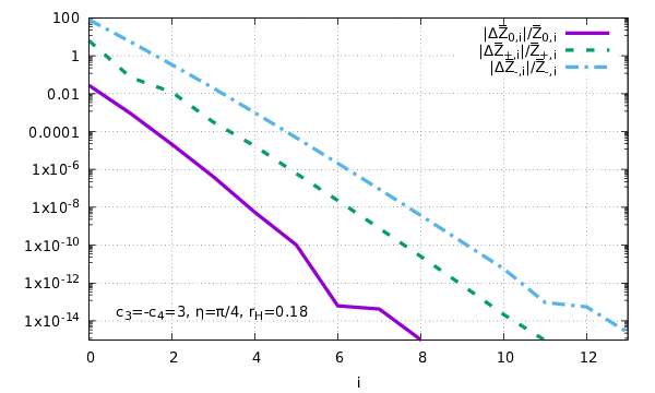

To see the convergence of the iterations, we compute for each and for each discretization point the difference of the results of the consecutive th and th iterations, and then we take the average over all discretization points. Computing similarly the average of , the ratios decrease with exponentially fast, as seen on the left panel in Fig.1, hence the iterations converge. The solution of the integral equations is shown on the right panel in Fig.1: the amplitudes and against (for ). One can see that the amplitude is always small but nonvanishing, and that all the three amplitudes vanish for , hence the solution is indeed asymptotically flat.
This yields an asymptotically flat solution in the region . To extend this solution to the region one only needs its values at ,
| (7.9) |
To recapitulate, the described above procedure yields the boundary values for the fields at a large and makes sure that the solution for exists and is indeed asymptotically flat. It is worth noting that the parameter determines the ADM mass,
| (7.10) |
VIII NUMERICAL PROCEDURE
Summarizing the above discussion, the asymptotically flat black holes are described by solutions of the three coupled first order ODEs (IV) for the three functions [which determines also ] with the following boundary conditions. At the horizon one has
| (8.1) |
where the horizon values and are finite and determined by the Eqs. (A.24), (A.22) in Appendix APPENDIX A: DESINGULARIZATION AT THE HORIZON, while can be arbitrary. Therefore, all possible boundary conditions at the horizon are labeled by just one free parameter , and choosing some value for it, the equations can be integrated directly from the horizon, as explained in Appendix APPENDIX A: DESINGULARIZATION AT THE HORIZON, to the outer region .
Far from the horizon, at , one has
| (8.2) |
where and are functions of determined by (VII) via iterating the integral equations (VII).
As a result, we have the boundary conditions at labeled by and the boundary conditions at labeled by . We use them to construct solutions in the region . To this end, we choose some value of and integrate numerically the equations starting from as far as some and we obtain at this point some values which will depend on and :
| (8.3) |
Then we choose and numerically extend the large data (VIII) from down to , thereby obtaining
| (8.4) |
If the two sets of values agree, hence if
| (8.5) |
then the solution in the interval merges smoothly with the solution in the interval to represent one single solution in the interval . The extension to the region is then provided by the integral equations (VII), finally yielding an asymptotically flat black hole solution in the region . It is worth noting that these solutions will depend neither on nor on ; these values could be varied without affecting the global solution (which is a good consistency check).
In some cases using just two zones and produces too large numerical errors. To keep the numerical instability under control, one should then integrate through many smaller zones , and perform matchings at (see Sec.7.3.5 in stoer). This yields numerically stable results.
In the case of just two zones, the problem reduces to solving the matching conditions (VIII) by adjusting the values . At least one solution to these three conditions certainly exists and corresponds to the Schwarzschild solution, for which
| (8.6) |
Are there other solutions ? Since there are three matching conditions for the three variables, their solutions must constitute a discrete set of points in the 3-space spanned by . This implies that different black hole solutions with the same are parametrically isolated from each other. This creates a problem, since in order to solve numerically algebraic equations (VIII), an input configuration is needed to start the numerical iterations within the Newton-Raphson procedure Press:2007:NRE:1403886. However, unless the input configuration is close to the solution, the numerical iterations do not converge, hence some additional information is necessary to specify where to start the iterations.
As explained in the Introduction, the additional information is provided by the stability analysis of the Schwarzschild solution (1.2) Babichev:2013una; Brito:2013wya. In this analysis one considers the two metrics of the form (IV) with
| (8.7) |
where while the perturbations are assumed to be small and depend on . It turns out that at the GL point, for , the perturbation equations admit a static solution (zero mode) for which depend only on and are bounded everywhere in the region while . This solution can be viewed as a perturbative approximation of a new solution that merges with the Schwarzschild solution for .
This suggests that to get new solutions of the matching conditions (VIII), one should choose the event horizon size to be close and choose the input configuration to be close to (8.6). Then the numerical iterations should converge to values which are slightly different from (8.6) and correspond to an almost Schwarzschild black hole slightly distorted by a massive hair. Changing then iteratively the value of yields solutions which deviate considerably from the Schwarzschild metric close to the horizon, but always approach flat metric in the asymptotic region.


IX ASYMPTOTICALLY FLAT HAIRY BLACK HOLES
Applying the procedure outlined above, we were able to construct asymptotically flat hairy solutions. We confirm the results of Ref. Brito:2013xaa and obtain many new results.
First of all, we find that for approaching from below the GL value, , there are asymptotically flat hairy black hole solutions for any . They are very close to the Schwarzschild solution: one has and the ADM mass . However, for smaller values of the solutions deviate more and more from Schwarzschild. To illustrate this, we plot in Fig. 2 the functions , , , , and . If these functions all equal to one, then the solution is Schwarzschild. As one can see, they indeed approach unity far away from the horizon, but close to the horizon they deviate considerably from unity, hence the massive graviton hair is concentrated in this region.


Solutions are regular for close to ; however, for smaller and depending on values of , the amplitudes may show additional zeros outside the horizon, whereas always remain positive. This implies that the f metric is singular, because the invariants of its Riemann tensor diverge where the zeros are located. An example of this is shown on the lower two panels in Fig. 2, and also on the lower two panels in Fig. 3 where one can see that the phenomenon occurs when approaches . The fact that the f metric becomes singular does not invalidate the solutions because the f-geometry is not directly measurable and its singularities are not seen, while the g metric, which can be probed by test particles, remains always regular. We shall therefore keep such solutions in our consideration.
Solutions in Fig. 2 are shown up to large but still finite values of the radial coordinate, or . What is shown is the combination of the solutions of differential equations (IV) in the region and of the integral equations (VII) for where . At the same time, our procedure yields solutions in the whole region . Introducing the compactified radial variable
| (9.1) |
we plot in Fig. 3 the amplitudes against . As seen, the amplitudes approach unity as (same is true for ) hence the solutions are indeed asymptotically flat. The disadvantage of this parametrization is that the slope of the functions does not vanish for . Indeed, for large one has and hence at infinity .


If then and the g metric becomes Schwarzschild. The theory reduces then to the massive gravity for the dynamical f metric on a fixed Schwarzschild background. The solution for the f metric is shown on the lower right panel in Fig. 3. Similarly, for one has and the f metric is Schwarzschild, while the g metric is a solution of the massive gravity on the Schwarzschild background shown on the upper left panel in Fig. 4. One should emphasize that the radii of the background Schwarzschild black holes for and for are not the same. For example, for the Schwarzschild black hole has for the solution shown in Fig. 3, while for the event horizon size is determined not by but by where (as seen in Fig.4) hence this time the Schwarzschild black hole is much larger. As a result, solutions on these different backgrounds look quite different – the solution for the f metric on the lower right panel in Fig. 3 shows zeros hence it is singular, while the solution for the g metric on the upper left panel in Fig. 4 is regular.
Solutions for will play an important role below. We shall call them “hairy Schwarzschild” because their g metric is Schwarzschild but their f metric supports hair.
Figure 4 shows the dependence of and of the ADM mass expressed in units of the Schwarzschild mass , as well as the temperature expressed in units of the Schwarzschild temperature . As one can see, the dependence is rather strong for small , in particular for . The decrease of the mass with can be understood by noting that the mass is the same with respect to each metric (the same is true for the temperature). If then the g metric is Schwarzschild hence and . If then the f metric is Schwarzschild with a larger radius , hence the mass is larger, , while the temperature is smaller, . Therefore, if then so that, for example, for , as seen in Fig. 4.
Figure 5 shows the dependence of and on in the case where . One can see that the solutions exist if only the value of is not too small. Similarly, not all hairy black holes exist for however small values of . As was noticed in Brito:2013xaa, small black holes exist if the coefficient in the potential (2.4) vanishes so that the cubic part of the potential is absent. In view of (2.15), this requires that , but this is not the only condition. Depending on the parameter values, one can distinguish the following two cases:
| (9.2) |
In case I asymptotically flat hairy black holes exist only if hence they cannot be arbitrarily small. In case II they exist for any , although their f metric may be singular for small . We shall see below in Sec. XI what happens when approaches the lower bound.


IX.1 Duality relation
The results described above in this section essentially reproduce those of Ref. Brito:2013xaa, the only important difference being that we show solutions for different values of , whereas Ref. Brito:2013xaa shows them only for . However, starting from this moment and in the following two Sections we shall be describing new results.
Reference Brito:2013xaa finds solutions only below the GL point, for . At the same time, the consistency of the procedure requires that there should be asymptotically flat hairy black holes also for . This follows from the symmetry (4.16) of the equations, which now reads
| (9.3) |
More precisely, this means that if for some values of there is a solution
| (9.4) |
then for , , there should be the “dual” solution described by
| (9.5) |
where is the function inverse for , such that . This duality correspondence relates between themselves black holes of different size, because (9.4) has the horizon at while the horizon of (9.5) is located where , that is at . One has
| (9.6) |
Now, for hairy solutions with one always has and . It follows that their duals are characterized by and by .
An explicit example of the duality relation is shown in Fig. 6, which presents on the left panel the solution for , , for which , hence . The duality implies that for , , there must be the dual solution with and , which is indeed confirmed by our numerics. Plotting the first solution against and the second one against , as shown in Fig. 6, yields exactly the same curves, up to the interchange , .
It is unclear why solutions with were not found in Brito:2013xaa.
The duality is in fact a powerful tool for studying the solutions, because sometimes their properties may look puzzling in one description but become obvious within the dual description.


X STABILITY ANALYSIS
In this section we analyze the stability of the hairy solutions by studying their perturbations within the ansatz described in Appendix APPENDIX B: FIELD EQUATIONS WITH TIME DEPENDENCE,
| (10.1) |
where , , , , , are functions of and . The full set of the field equations in this case is shown in Appendix APPENDIX B: FIELD EQUATIONS WITH TIME DEPENDENCE. If we set and assume that nothing depends on time, then we return back to the static case studied above. Therefore, small deviations from the static solutions are described by (X) with
| (10.2) | ||||
where the functions , , , , correspond to the background black hole solution while the perturbations are small.
We therefore inject (X) to Eqs.(APPENDIX B: FIELD EQUATIONS WITH TIME DEPENDENCE) and (B.36) and linearize with respect to the perturbations. Linearizing the equation yields
| (10.3) |
where relate to the static background, and we do not write their over sign “” for simplicity. In the linear perturbation theory one can consistently separate the time variable by assuming the harmonic time dependence for all amplitudes (this would no longer be possible if non-inear corrections are taken into account), so that we choose
| (10.4) |
and similarly for . Injecting to (10.3) yields the algebraic relation
| (10.5) |
Linearizing similarly the equation yields a linear relation between , , . Using these two algebraic relations one finds that the three equations , and yield upon the linearization three equivalent to each other relations. Therefore, among the 8 equations (APPENDIX B: FIELD EQUATIONS WITH TIME DEPENDENCE), (B.36) only 6 are independent (at least at the linearized level).
Taking all of this into account and linearizing similarly the remaining 3 equations , and , one finds that all 6 perturbation amplitudes , , , , and can be expressed in terms of a single master amplitude subject to the Schrödinger-type equation,
| (10.6) |
The master amplitude is a linear combination of and with rather complicated coefficients whose explicit expression is not particularly illuminating, hence we do not show it explicitly. The potential is also a complicated function of the background amplitudes that we do not show. The tortoise radial coordinate is defined by the relation
| (10.7) |
where the function (also complicated) varies from to as changes from to . The potential always tends to zero at the horizon, for , and it approaches unit value at infinity, for . One should remember that our dimensionless variables are related to the dimensionful ones via mr, , , .
For the bald Schwarzschild background with and , one has and the potential reduces to
| (10.8) |
in agreement with Ref. Brito:2013wya. In the flat space limit this reduces to , which is the potential of a massive particle of unit mass (in units of the graviton mass) with spin .
Equation (10.6) defines the eigenvalue problem on the line . Solutions of this problem with describe scattering states of gravitons. In addition, there can be bound states with purely imaginary frequency and hence with . For such solutions the wave function is everywhere bounded and square-integrable, because one has as , respectively. Such bound state solutions grow in time as . Therefore, they correspond to unstable modes of the background black holes.
X.1 Computing the eigenfrequencies
Our aim is to investigate a potential existence of negative modes with in the spectrum of the eigenvalue problem (10.6). If such modes exist, then the background black holes are unstable. If they do not exist, then the black holes are stable with respect to spherically symmetric perturbations, which would strongly suggest that they should be stable with respect to all perturbations. Indeed, in most known cases the -channel is usually the only place where the instability can reside (of course, this should be proven case to case).


The first thing to check is the shape of the potential , because if it is everywhere positive, then there are no bound states. We therefore show in Fig. 7 the potential for the hairy backgrounds for several values of the event horizon size and for different , and we also show for the bald Schwarzschild solution with the same (it does not depend on ). We observe that in each case the potential vanishes at the horizon, then shows negative values in its vicinity, and then approaches unity as . Since the potential is not positive definite, bound states may exist, but their existence is not yet guaranteed.
We know that a bound state certainly exists for the bald Schwarzschild background with Babichev:2013una; Brito:2013wya. When looking at the potentials for the hairy solution with in Fig. 7, we notice that they are close to the Schwarzschild potential, hence a bound state could exist for these potentials as well.
In order to know whether bound states exist or not, we use the well-known Jacobi criterion gelfand2000calculus and construct the solution of the Schrödinger equation (10.6) with . If this solution crosses zero somewhere, then there are bound states. We start in the asymptotic region where the tortoise coordinate becomes identical to the usual , hence Eq.(10.6) reduces simply to so that the bounded solution is . Then we extend this solution numerically toward small values of , and we find that, depending on values of , it may indeed show a zero as approaches . Therefore, there exists a bound state.


The next step is to actually find the bound state by solving the eigenvalue problem (10.6) with the potential obtained by numerically solving the background equations. For this we set and determine the local solutions at infinity and close to the horizon,
| (10.9) |
where is an integration constant. Then we apply the multiple shooting method and numerically extend the horizon solution toward large , extending at the same time the large solution toward small . The two solutions meet at some intermediate point , where the values of and should agree. This gives two conditions to be fulfilled by adjusting the two parameters and in (10.9), which finally yields the bound state solution on the whole line (see Pani:2013pma; Berti:2009kk for a review on the black hole perturbation theory and the tools that can be used to solve the perturbation equation).
The eigenfunctions against the ordinary radial coordinate are shown in Fig. 8. They vanish at the horizon, then show a maximum, sometimes very close to the horizon, and then approach zero for .
As a result, we find the negative eigenvalues for all hairy black holes obtained in Brito:2013xaa. Therefore, all these solutions are unstable. It is worth emphasizing that all of them correspond to the particular choice , hence . In order to test our method, we have also computed the negative mode for the bald Schwarzschild solution as in Brito:2013wya.
As seen in Fig. 9, the absolute value of the negative mode eigenvalue for the Schwarzschild solution is always larger than that for the hairy solutions. Therefore, the instability growth rate for the hairy black holes is not as large as for the Schwarzschild solution. In all cases, since one has where is the dimensionful physical frequency, the instability growth time is . If we assume the graviton mass to be very small and given by (5.5), then the instability growth time will be cosmologically large, hence the instability will not play any role. However, as we shall see below, it is preferable to assume that km according to (5.8), in which case the instability growth time will be less than seconds, hence the instability is dangerous and should be avoided.

As seen in Fig.9, the eigenvalue approaches zero when , therefore all hairy black holes become then stable. However, they are no longer hairy in this limit, because they “lose their hair” and merge with the bald Schwarzschild solution. Near all solutions are close to each other and is close to zero for any , while for smaller the backgrounds and become parameter dependent. The eigenvalue may approach zero also for type I solutions for a small when they cease to exist. For example, for , , the hairy solution disappears at , and at the same time the eigenvalue approaches zero, as seen in the insertion in Fig. 9.
The instability of hairy black holes is in fact a somewhat puzzling phenomenon, since it is unclear what they may decay into. Since the hairy solutions with are more energetic than the bald Schwarzschild solution, they probably may approach the latter via absorbing and/or radiating away their hair during their decay. However, the bald Schwarzschild solution is also unstable for and should decay into something.
The perturbative instability of the Schwarzschild solution in the massive bigravity theory is mathematically equivalent Babichev:2013una to the Gregory-Laflamme instability of the vacuum black string in D=5 Gregory:1993vy. It is known that the nonlinear development of the latter leads to the formation of an infinite string of “black hole beads” in , but the event horizon topology does not change Lehner:2011wc. This fact being established within the vacuum GR, a similar scenario is not possible in the bigravity theory, hence the fate of the bigravity black holes should be different. One possibility is that the black hole radiates away all of its energy within the S-channel (some radiative solutions are known explicitly Kocic:2017hve; Hogas:2019cpg), but it is unclear what happens to the horizon, whether it disappears or not. In GR the horizon cannot disappear via a classical process Hawking:1973uf, but in the bimetric theory the situation might be different.
Remarkably, we find that these puzzling issues are not omnipresent and the black holes can be stable if is different from . In Fig. 10 we show against for several values of for solutions with . One can see that approaches zero and the negative mode disappears in the hairy Schwarzschild limit when approaches . At the same time, the bald Schwarzschild solutions for the same are certainly unstable. This is a very encouraging fact – we see that adding the hair to the black hole provides the stabilizing effect. As is seen in Fig. 10, the eigenvalue approaches zero also when become small, if only is also small, as seen in Fig. 10.
Summarizing the above discussion, for some parameter values the hairy black holes are unstable, but for other parameter values they can be stable. Below we shall describe a parameter choice leading to a large set of stable solutions.

XI PARAMETER SPACE AND THE PHYSICAL SOLUTIONS
In this section we give a detailed description of particular subsets of solutions. Providing a complete classification of solutions depending on 4 parameters would be a very difficult task. We therefore adopt the following strategy: choosing the particular values
| (11.1) |
which fulfill condition II in (9.2), we study the solutions for all possible . Performing next the duality transformation gives us all possible solutions for
| (11.2) |
which values fulfill condition I in (9.2). This approach reveals interesting and rather complex features which are presumably generic for any .
Figure 11 shows the ADM mass and the function for several values of . As one can see, all curves intersect at the GL point, , where all solutions bifurcate with the bald Schwarzschild solution,
| (11.3) |
whereas all curves pass through the point . Away from the bifurcation point, the g metric still remains Schwarzschild if , in which case is a linear function,
| (11.4) |
but the f metric for these solutions is not Schwarzschild, even though both metrics have the same mass; as explained above, we call such solutions hairy Schwarzschild. For the mass depends nonlinearly on .


Introducing the mass function via , Eq.(4.3) assumes the form
| (11.5) |
from where the ADM mass
| (11.6) |
Here the “bare” mass is determined only by the horizon radius and coincides with the mass of the Schwarzschild solution of radius , whereas the mass expressed by the integral is the contribution of the massive hair distributed outside the horizon. As one can see in Fig. 11, one has if , hence the “hair mass” is positive and the hairy solutions are more energetic than the bare Schwarzschild black hole. However, the mass of the hair becomes negative above the GL point, where , and the hairy solutions are then less energetic than the bare one. Therefore the energy density can be negative. In fact, there are no reasons for which the standard energy conditions should be respected within the bigravity theory.
Each curve in Fig. 11 is defined only in a finite interval . It is very instructive to understand what happens at the boundaries of this interval.
XI.1 The lower limit
All the solutions extend down to arbitrarily small values of . Remarkably, as seen in Fig. 11, except for the mass does not vanish when but approaches a finite value, even though the bare mass . Therefore, all mass is contained in the hair mass in this limit, hence something remains even when the horizon size shrinks to zero. A similar phenomenon is actually well known, since in many nonlinear field theories there are solutions describing a small black hole inside a soliton (for example, inside the magnetic monopole) Volkov:1998cc. Sending the horizon size to zero the black hole disappears, but its external nonlinear matter fields remain and become a gravitating soliton containing a regular origin in its center instead of the horizon. Therefore, the limit of a hairy black hole may correspond to a regular soliton.
One may expect the situation to be similar also in our case and that there is a limiting configuration to which the black hole solutions approach pointwise when . Such a limiting configuration indeed exists; however it seems to be singular and not of the regular soliton type. First, as seen in Fig. 11, the value of which determines the size of the f horizon remains finite when , hence the f geometry remains a black hole even in the limit. Secondly, as seen in Fig. 12, one has for for a solution with a very small . However, one has as , hence one has in this limit and the limiting form of the g metric is something like a “zero size black hole”. The numerical profiles shown in Fig. 12 suggest this limiting configuration to have the following structure at small :
| (11.7) |
The g geometry is singular since its Ricci invariant at small , but the f geometry remains of the regular black hole type because does not vanish. Curiously, the temperature remains finite for and is always the same for both metrics. The limiting g temperature can be formally computed by assuming , with and from Fig. 12. Equation (6.5) then yields , which is very close to the value for the solution with shown in Fig. 12. However, these considerations are of course purely formal since the zero size black hole cannot evaporate and further reduce its size, and the standard WKB arguments for the black hole evaporation do not apply because the geometry is singular at the horizon.


One should say that the f metric can become singular for small because the amplitudes develop additional zeros outside the horizon. This happens along the parts of the curves on the left of the points marked by the crosses in Fig.11. We have already discussed this phenomenon and said that we do not exclude such solutions from consideration because the f geometry is not observable and its singularities are invisible, while the g geometry that can be directly probed remains always regular. The physical parameters of the solutions such as the ADM mass also do not show anything special when the amplitudes starts to oscillate. The potential in the perturbation equation (10.6) also remains regular. We therefore have no reason to exclude such solutions from consideration, and in fact they are necessary in order that the theory could describe black holes within a broad mass spectrum.
XI.2 The upper “tachyon” limit
In this limit the solutions always remain regular and disappear after a fusion of roots of the algebraic equation (6.3) [or (A.24)]. As explained above, this equation determines the horizon values of the solutions. Its two roots determine two solution branches, but only the root with gives rise to asymptotically flat solutions, the other branch showing a singularity of the g metric outside the horizon. When increases, the determinant of (6.3) decreases and vanishes for some , then it becomes positive again, decreases again and vanishes for the second time for , after which it becomes negative and the procedure stops. Specifically, it turns out that the determinant of (6.3) factorizes,
| (11.8) |
where is defined by (3.5) with replaced by while is a complicated function of . When increases, then crosses zero at some while remains positive, hence the square root changes sign. When continues to increase, then approaches zero and vanishes as . No further increase of is possible since would then be negative thus rendering the solutions complex valued.
Although the determinant vanishes for when and also for when , the two solution branches never merge. Specifically, the two horizon values determined by (A.24) merge when , but a careful inspection reveals that in (A.21) and (A.22) remain different for the two branches when . If then all horizon values coincide for the two branches, but the derivatives defined by (A.28) remain different. This is a consequence of the fact that the existence and uniqueness theorem applies only to regular points of the differential equations, whereas the event horizon is a singular point.
In the interval the solutions show a “tachyon zone” near the horizon where the function defined by (3.5) is negative, as shown in the right panel in Fig. 12. Let us remember relation (2.13) for the Fierz-Pauli mass of gravitons obtained via linearizing the field equations around the flat background. This relation can be written as . However, the equations can be similarly linearized around an arbitrary background solution, which yields in the spherically symmetric case the position-dependent mass term Mazuet:2018ysa
| (11.9) |
Therefore, if then the mass effectively becomes imaginary. As a result, solutions for show unphysical features, hence we call the “tachyon limit”. The horizon value diverges in this limit, but this seems to be an integrable divergence similar to and the limiting solution itself stays regular. We were able to approach this solution rather closely, as shown in Fig. 12 (right panel) which presents “an almost limiting” solution with the horizon value of the determinant .
To recapitulate, hairy solutions exist only for .
XI.3 The ADM mass
It is important that, unless is very small, the ADM mass of all hairy solutions always varies within a finite range and can be neither very large nor very small, as seen in Fig. 11. It seems this fact was not recognized in Ref. Brito:2013xaa, which always shows only the ratio which diverges as . However, the mass remains finite for . As seen in Fig. 11, the mass actually does not change much when changes and always remains close to the GL value, which is the mass of the Schwarzschild solution with ,
| (11.10) |
This means that the dimensionful mass (restoring for the moment the speed of light and Newton’s constant )
| (11.11) |
is always close to that of the Schwarzschild black hole of size , which is close to the Compton length of massive gravitons. As a result, one cannot assume the graviton mass m to be very small and of the order of the inverse Hubble radius as in (5.5). Indeed, this would imply the hairy black holes to be as heavy as the Schwarzschild black hole of a cosmological size – a physically meaningless result. However, assuming instead that km with as in (5.8), which is consistent with the cosmological observations if is parametrically small as expressed by (5.6), yields a physically acceptable result. The masses of the hairy black holes are then close to the mass of the Schwarzschild black hole of radius km, that is . If this gives the value typical for supermassive astrophysical black holes observed in the center of many galaxies.
If is very small then the mass can deviate considerably from the GL value and can become very small or very large. As seen in Fig. 11, for small the mass shows a minimum: first it decreases with , then reaches a minimal value , and then increases up to some . For smaller values of the minimum becomes more and more profound and the value approaches zero while becomes larger and larger. If is extremely small as in (5.6), , then the minimum value is extremely close to zero. One has then for where is very small, but in the region the mass grows rapidly when up to a very large value .


To get an approximation for for very small , we consider the hairy Schwarzschild solutions with . Their g metric is Schwarzschild with all the hair contained in the f metric. It turns out that the amplitudes of the f metric depend very strongly on if the latter is small. As seen in Fig. 13, in the horizon vicinity these amplitudes show very large values which apparently grow without bounds when , although one always has and far away from the horizon. We inject these solutions to (11.5) and (11.6) to obtain the radial energy density and . They also become very large when decreases, as seen in Fig. 13. The asymptotic value is the “hair energy”. As seen in Fig. 13, the hair energy is large for small , but it does not backreact and the g metric remains Schwarzschild if . However, the hair energy starts to backreact if . If then one can deduce from Eq.(11.6) that
| (11.12) |
where is computed for . We evaluate numerically for various values of and obtain the following best fit approximation:
| (11.13) |
where and . Assuming that , this function shows an absolute minimum at
| (11.14) |
whose dimensionful versions are obtained by multiplying by km (restoring again the speed of light and Newton’s constant)
| (11.15) |
This determines the minimum mass for the hairy black holes. When gets smaller still then the mass starts to grow, but it grows only up to a finite although very large value as because the approximation (11.13) is not valid for however small .
XI.4 Parameter regions for solutions with
Let us now collect all the facts together. The diagram in Fig. 14 shows the region in the plane within which there are hairy black hole solutions. The low boundary of this region at corresponds to solutions whose f metric is Schwarzschild, while the upper boundary at corresponds to solutions whose g metric is Schwarzschild. The left boundary corresponds to the limiting solutions with : the zero size black holes. The right boundary marks the “tachyon limit” beyond which the solutions would become complex valued. The upper-left corner of the diagram contains solutions with a singular f geometry, but their g geometry, which is physically measurable, is regular.
The diagram also shows lines corresponding to the zero modes, , of the perturbative eigenvalue problem (10.6). The vertical line corresponds to the GL value . The eigenvalue changes sign when crossing these lines, therefore, the lines separate sectors where and hence the solutions are stable, from sectors where and the solutions are unstable. There are altogether two stable and two unstable sectors. It is worth noting that the stability region is now much larger than for solutions with considered in the previous section. One also notices that the tachyonic solutions are in the unstable sector.

Finally, the diagram shows the “physical region” corresponding to physically acceptable solutions. As explained above, for such solutions the coupling should be very small for their mass not to be too large, hence should be very close to . The solutions should be stable, hence they should correspond to the sector where . These conditions specify the physical region to be the thick (green online) line at the top of the diagram.
Physical solutions are therefore described by the g metric which is extremely close to Schwarzschild, since
| (11.16) |
The “hairy features” of the solutions hidden in the f metric should be difficult to observe, unless in violent processes like black hole collisions producing large enough to overcome the suppression. Summarizing, the static bigravity black holes should be extremely similar to the GR black holes, but their strong field dynamics is expected to be different.
As explained above, the physical region contains stable hairy black holes whose masses range from the minimal value up to the maximal value with . Yet heavier black holes also exist in the theory but they cannot be hairy and should be described by the “bald” Schwarzschild solution (1.2), which is stable for . Stable black holes with can only be of the type (1.1).
XI.5 Parameter regions for dual solutions with ,
Let us now see how the described above solutions look after the duality transformation (9.3). This transformation converts the parameter values (11.1) into (11.2), flips the sign of and swaps the with . Graphically, this amounts to relabelling the functions and plotting them against instead of . The ADM mass and temperature are invariant under duality. The stability property also does not change since, for example, if a solution is unstable and admits growing in time perturbations, then its dual version will contain the same growing modes and hence will be unstable as well.


Figure 15 shows the dual version of Fig. 11. The mass curves still intersect in the GL point but they look quite different as compared to those in Fig. 11. In particular, not all of them are single valued. The reason is that the functions in Fig. 11 are not always monotone, hence their inverses shown in Fig. 15 are not single-valued. As a result, for each such that there are two different solutions with the same but with different , hence the curves are not always single valued.
The solutions now exist for . The lower limit corresponds to what used to be the upper limit before the duality – the tachyon solutions with vanishingly small horizon determinant . The upper limit corresponds for small to solutions whose g metric starts being singular. Before the duality these were solutions whose f metric started being singular while their g-metric was regular. After the duality their g-metric becomes singular, hence such solutions are no longer allowed and should be excluded. For larger values of the right boundary corresponds to points where the two different solutions with the same but with different merge to each other.
The solutions below the GL point, for , are still more energetic than the solution with , hence their hair mass is positive, whereas above the GL point it becomes negative. Finally, Fig. 16 shows the existence diagram in the plane, together with the stability regions. The diagram now looks quite different as compared to that in Fig. 11, although it corresponds to essentially the same solutions, up to the duality transformation. Although the duality does not change stability, it interchanges positions of the stability sectors. Therefore, the physical region corresponding to stable solutions with close to is now above the GL point, where the hair mass is negative. The physical solutions are again characterized by the g metric that is extremely close to Schwarzschild, but the novel feature is that now for each value of from the physical region there are two different solutions whose g metrics are almost the same but the f metrics are different.
As one can see, the physical region in Fig.15 is rather short and corresponds only to supermassive black holes with . All black holes of smaller masses are unstable. Therefore, the parameter choice , is not physically interesting.

XII CONCLUDING REMARKS
To recapitulate, we presented above a detailed analysis of static and asymptotically flat black holes in the ghost-free massive bigravity theory. Extending the earlier result of Brito:2013xaa, we find that for given values of the theory parameters and for a given event horizon size varying within a finite range, , there are one or sometimes two different black holes supporting a nonlinear massive graviton hair, in addition to the “bald Schwarzschild” solution with described by (1.2). The hairy solutions are more energetic than the Schwarzschild one if and they are less energetic otherwise. When approaches the limiting values or , the solutions either become complex valued or merge between themselves. For some values of zero-size black holes exist for which but the corresponding remains finite. Depending on values of , the hairy solutions can be either stable of unstable.
To avoid the hairy black holes being unphysically heavy, one is bound to assume the massive graviton Compton length to be km where the parameter may range in the interval . The agreement with the cosmological data is then achieved by assuming that . The stable hairy black holes are described by a g metric which is extremely close to Schwarzschild, but their f metric is quite different. These black holes have the mass and size close to those of ordinary black holes with the masses ranging from to , the latter being the value typical for the supermassive astrophysical black holes if . Yet heavier black holes in the theory should be bald. As a result, if the bigravity theory indeed applies to describe physics, the astrophysical black holes should support the hair hidden in the f metric.
Since the f metric is not coupled to matter and cannot be directly probed, while the deviation of the “visible” g metric from Schwarzschild is suppressed by the factor of , the hairy black holes should normally be undistinguishable from the usual GR black holes. However, in violent processes like black hole coalescences the interaction between the two metrics may produce an energy momentum tensor strong enough to overcome the suppression in . In this case the deviation from GR should become visible. Therefore, it is possible that signals from black hole mergers detected by LIGO/VIRGO Abbott:2016blz may carry information about the hairy structure of the black holes. One could expect a “hair imprint” in the signal to be stronger for small black holes, since we know that for small black holes the amplitudes of the f metric become very large, which should influence the of the merger. It is therefore possible that the hair imprints will be visible when smaller mass mergers (see Abbott:2020niy for a recent review) are detected. However, to actually determine the hair imprint in the signal would require calculations going beyond the scope of the present paper. We therefore leave this problem for a separate project and for the time being simply refer to the recent preprint Dong where calculations of this type are performed within the context of the ghost-gree massive gravity deRham:2010kj [where the only static black holes are those described by (1.1)].
Finally, we should discuss the paper Torsello:2017cmz that also considers black holes in the ghost-free massive bigravity theory. This paper presents essentially the same classification of different types of black holes as the one previously given in Volkov2012 but in a more refined way, extending it and paying attention to some subtle points. The paper addresses in particular the issue of convergence of the solutions to the flat background in the asymptotic region. Among other things, it claims that the Schwarzschild solution is the only asymptotically flat black hole in the theory. At the same time, the paper does not contain a rigorous proof of this statement but gives just a number of plausibility arguments, so that the claim should rather be viewed as a conjecture, as actually explicitly stated in some places of Torsello:2017cmz. These arguments are as follows.
First of all, it was emphasized in Torsello:2017cmz that the usual practice of starting the numerical integration not at the horizon , which is a singular point of the differential equations, but at a regular nearby point , as was done in Brito:2013xaa, could in principle lead to numerical instabilities. We agree with this, and it is for this reason that we use the desingularization procedure (described in Appendix APPENDIX A: DESINGULARIZATION AT THE HORIZON below) which allows us to start the numerical integration exactly at (initial conditions exactly at were described also in Torsello:2017cmz).
The paper Torsello:2017cmz makes also another remark concerning the behavior at the horizon. It is known that in order to be able to cross the horizon, for example when studying geodesics, one cannot use the Schwarzschild coordinates and one should introduce instead regular at the horizon coordinates. These can be, for example, Eddington-Finkelshtein (EF) coordinates in which , . It was noticed in Torsello:2017cmz that the f metric, when expressed in the same coordinates, generically does not have the same form, since it has , hence the two metrics cannot be simultaneously EF. We understand this, but this does not invalidate the background solutions (Ref. Torsello:2017cmz agrees on this). The horizon geometries are regular, and if one wishes, one can use the same boundary conditions at the horizon to integrate inside the horizon to recover the interior solutions. Within the parametrization described in Appendix APPENDIX A: DESINGULARIZATION AT THE HORIZON, this is achieved by simply changing the sign of the numerical integration step.
Next, small initial deviations from the Schwarzschild solution via setting at the horizon were considered in Torsello:2017cmz. Integrating the equations toward large then yields metrics whose components diverge as instead of approaching finite values. This observation, made already in Volkov2012, shows that there are no regular and asymptotically flat solutions in a small vicinity of the Schwarzschild solution. However, there can be regular solutions corresponding to considerably deviating from unit value.
Finally, the paper Torsello:2017cmz reproduces and analyzes (in Appendix A) one of the asymptotically flat solution (with a singular f metric) found in Brito:2013xaa. It obtains a pathological result, and the reason is the following. Appendix D of Torsello:2017cmz describes the numerical method used – a straightforward integration starting from the horizon with the standard routine of Mathematica. This adequately produces the solution with a given precision, but only within a finite range of the radial coordinate . If one integrates farther on trying to approach flat space, then the growing mode generically present in the solution leads to a rapid accumulation of numerical errors triggering a numerical instability. Trying to suppress this mode by adjusting the horizon boundary conditions, one typically observes the derivatives of some functions in the solution growing without bounds at a some finite . Precisely this type of behavior at the end of the integration interval is seen in Fig. 11 in Torsello:2017cmz.
One cannot get asymptotically flat solutions within the numerical scheme adopted in Torsello:2017cmz, since pathological features arise in this way inevitably. This must be the reason behind the conviction that such solutions do not exist. However, all pathologies can be eliminated within the more elaborate numerical scheme described above – via suppressing the growing mode from the very beginning.
ACKNOWLEDGEMENTS
We thank Francesco Torsello, Mikica Kocic and Edvard Mörtsell for clarifying discussions and useful remarks. The work of M.S.V. was partly supported by the French National Center of Scientific Research within the collaborative French-Russian research program, Grant No. 289860, as well as by the Institute of Theoretical and Mathematical Physics at the Moscow University during the visit in early 2020, and also by the Russian Government Program of Competitive Growth of the Kazan Federal University.
APPENDIX A: DESINGULARIZATION AT THE HORIZON
The horizon is a singular point of the differential equations – the derivatives and expressed by Eqs.(IV) are not defined at this point. The usual practice to handle this difficulty is to use the local power series expansions (VI) and (6.2) to start the numerical integration not exactly at but at a nearby point with where is a small number. One may then hope that the results will not be very sensitive to the value of . However, in such an approach remains an arbitrary parameter not defined by any prescription. This inevitably affects the stability of the numerical procedure, which becomes evident when one studies the dependence of the solutions on the parameters.
At the same time, it is possible to reformulate the problem in such a way that the numerical integration starts exactly at . Let us make the change of variables
| (A.17) |
The functions and their derivatives are defined also at . Equations (4.3) and (4.4) then yield
| (A.18) |
where
| (A.19) |
At the horizon the derivatives and are finite, which requires that
| (A.20) |
from where one obtains the horizon values
| (A.21) | |||||
| (A.22) |
At the same time, the horizon value of can be obtained from (IV),
| (A.23) |
This value must agree with the one given by (A.21), which yields a condition on , and using (A.22), this condition reduces [if are chosen according to (2.15)] to a biquadratic equation
| (A.24) |
where the coefficients , , are (rather complicated) functions of . As a result, for given there are two possible horizon values and . Injecting to (A.21) and (A.22), this determines the horizon values and . Finally, the horizon values of and are obtained from (A.18) by taking the limit and using l’Hopital’s rule, which yields
| (A.25) |
There remains to compute the derivatives here. One has, for example,
| (A.26) |
where the second derivative is similarly obtained from (A.23),
| (A.27) |
and similar expressions for . Injecting this to (A.25) yields linear in and relations, which can be resolved to give (we do not show explicit formulas in view of their complexity)
| (A.28) |
Summarizing the above discussion, the equations in the desingularized form read
| (A.29) |
where and are defined by (APPENDIX A: DESINGULARIZATION AT THE HORIZON) while is the same as in (IV). These equations apply for , while at they should be replaced by
| (A.30) |
where , , are defined by Eqs.(A.21) and (A.28). The horizon values and can be arbitrary, while is not arbitrary but must fulfil the algebraic equation (A.24), whereas is determined by (A.22). This formulation allows one to start the integration exactly at the horizon and then continue to the region.
APPENDIX B: FIELD EQUATIONS WITH TIME DEPENDENCE
Let us allow both metrics to depend on time, assuming that they are still spherically symmetric. The gauge freedom of reparametrizations of the coordinates can be used to make the g metric diagonal, but the f metric will in general contain an off-diagonal term. The two metrics can be written as Volkov:2011an
| (B.31) |
where and , , , , , , are functions of and .
One can check that the tensor
| (B.32) |
has the property . This tensor is used to compute the energy-momentum tensors and in (2.7).
One can redefine the two amplitudes similarly to (4.1)
| (B.33) |
where the prime denotes the derivative with respect to , and one can impose the gauge condition
| (B.34) |
As a result, the independent field equations (2.18) become
| (B.35) |
plus two nontrivial components of the the conservation condition,
| (B.36) |
Here one has explicitly
| (B.37) |
where the dot denotes the partial derivative with respect to , while
| (B.38) |
where are defined in (3.5). The components of the second stress-energy tensor are
| (B.39) |
where . The components of the Einstein tensor for , are complicated:
| (B.40) |
Finally, there are two nontrivial components of the conservation law,
| (B.41) |
where are defined in (4.10). Equations (APPENDIX B: FIELD EQUATIONS WITH TIME DEPENDENCE), (B.36) comprise a system of 8 equations for 6 functions , , , , , . For this system not to be overdetermined, only 6 equations out of 8 should be independent. As shown in Sec. X, this indeed happens at least for small , when the perturbative analysis of the equations shows that some of them coincide.
References
- (1) A. Riess et al., Observational evidence from supernovae for an accelerating universe and a cosmological constant, Astron.Journ. 116 (1998), no. 3 1009, [doi.org/10.1086/300499].
- (2) S. Perlmutter et al., Measurements of and from 42 high-redshift supernovae, Astrophys.Journ. 517 (1999), no. 2 565, [doi.org/10.1086/307221].
- (3) M. Fierz and W. Pauli, On relativistic wave equations for particles of arbitrary spin in an electromagnetic field, Proc.Roy.Soc.Lond. A173 (1939) 211–232, [doi:10.1098/rspa.1939.0140].
- (4) H. van Dam and M. J. G. Veltman, Massive and massless Yang-Mills and gravitational fields, Nucl. Phys. B22 (1970) 397–411, [doi:10.1016/0550-3213(70)90416-5].
- (5) V. I. Zakharov, Linearized gravitation theory and the graviton mass, JETP Lett. 12 (1970) 312, [https://ui.adsabs.harvard.edu/abs/1970JETPL..12..312Z/abstract].
- (6) A. I. Vainshtein, To the problem of nonvanishing gravitation mass, Phys.Lett. B39 (1972) 393–394, [doi:10.1016/0370-2693(72)90147-5].
- (7) D. G. Boulware and S. Deser, Can gravitation have a finite range?, Phys.Rev. D6 (1972) 3368–3382, [doi:10.1103/PhysRevD.6.3368].
- (8) C. de Rham, G. Gabadadze, and A. Tolley, Resummation of massive gravity, Phys.Rev.Lett. 106 (2011) 231101, [arXiv:1011.1232], [doi:10.1103/PhysRevLett.106.231101].
- (9) S. F. Hassan and R. A. Rosen, Bimetric Gravity from Ghost-free Massive Gravity, JHEP 02 (2012) 126, [arXiv:1109.3515], [doi:10.1007/JHEP02(2012)126].
- (10) M. Volkov, Cosmological solutions with massive gravitons in the bigravity theory, JHEP 1201 (2012) 035, [arXiv:1110.6153], [doi:10.1007/JHEP01(2012)035].
- (11) M. von Strauss, A. Schmidt-May, J. Enander, E. Mortsell, and F. Hassan, Cosmological solutions in bimetric gravity and their observational tests, JCAP 1203 (2012) 042, [arXiv:1111.1655], [doi:10.1088/1475-7516/2012/03/042].
- (12) D. Comelli, M. Crisostomi, F. Nesti, and L. Pilo, FRW cosmology in ghost free massive gravity, JHEP 1203 (2012) 067, [arXiv:1111.1983], [doi:10.1007/JHEP06(2012)020, 10.1007/JHEP03(2012)067].
- (13) Y. Akrami, S. Hassan, F. Könnig, A. Schmidt-May, and A. R. Solomon, Bimetric gravity is cosmologically viable, Phys. Lett. B 748 (2015) 37–44, [arXiv:1503.07521], [doi:10.1016/j.physletb.2015.06.062].
- (14) E. Mortsell and J. Enander, Scalar instabilities in bimetric gravity: The Vainshtein mechanism and structure formation, JCAP 10 (2015) 044, [arXiv:1506.04977], [doi:10.1088/1475-7516/2015/10/044].
- (15) K. Aoki, K.-i. Maeda, and R. Namba, Stability of the Early Universe in Bigravity Theory, Phys. Rev. D 92 (2015), no. 4 044054, [arXiv:1506.04543], [doi:10.1103/PhysRevD.92.044054].
- (16) M. Lüben, E. Mörtsell, and A. Schmidt-May, Bimetric cosmology is compatible with local tests of gravity, Class. Quant. Grav. 37 (2020), no. 4 047001, [arXiv:1812.08686], [doi:10.1088/1361-6382/ab4f9b].
- (17) M. Högås, F. Torsello, and E. Mörtsell, On the stability of bimetric structure formation, JCAP 04 (2020) 046, [arXiv:1910.01651], [doi:10.1088/1475-7516/2020/04/046].
- (18) M. S. Volkov, Hairy black holes in the ghost-free bigravity theory, Phys. Rev. D85 (2012) 124043, [arXiv:1202.6682], [doi:10.1103/PhysRevD.85.124043].
- (19) S. V. Sushkov and M. S. Volkov, Giant wormholes in ghost-free bigravity theory, JCAP 1506 (2015), no. 06 017, [arXiv:1502.03712], [doi:10.1088/1475-7516/2015/06/017].
- (20) M. Volkov, Self-accelerating cosmologies and hairy black holes in ghost-free bigravity and massive gravity, Class.Quant.Grav. 30 (2013) 184009, [arXiv:1304.0238], [doi:10.1088/0264-9381/30/18/184009].
- (21) C. Isham and D. Storey, Exact Spherically Symmetric Classical Solutions for the F-G Theory of Gravity, Phys. Rev. D 18 (1978) 1047, [doi:10.1103/PhysRevD.18.1047].
- (22) M. Gurses, A new class of f-g fields relevant to quark confinement, Phys. Rev. D 20 (1979) 1019–1021, [doi:10.1103/PhysRevD.20.1019].
- (23) M. Gurses, Solutions of the f-g field equations, J. Phys. A 14 (1981) 1957–1971, [doi:10.1088/0305-4470/14/8/020].
- (24) C. Isham, A. Salam, and J. Strathdee, F-dominance of gravity, Phys.Rev. D3 (1971) 867–873, [doi:10.1103/PhysRevD.3.867].
- (25) E. Babichev and A. Fabbri, Stability analysis of black holes in massive gravity: a unified treatment, Phys. Rev. D 89 (2014), no. 8 081502, [arXiv:1401.6871], [doi:10.1103/PhysRevD.89.081502].
- (26) M. S. Volkov, Hairy black holes in theories with massive gravitons, Lect. Notes Phys. 892 (2015) 161–180, [arXiv:1405.1742], [doi:10.1007/978-3-319-10070-8_6].
- (27) Z. Berezhiani, D. Comelli, F. Nesti, and L. Pilo, Exact Spherically Symmetric Solutions in Massive Gravity, JHEP 07 (2008) 130, [arXiv:0803.1687], [doi:10.1088/1126-6708/2008/07/130].
- (28) D. Comelli, M. Crisostomi, F. Nesti, and L. Pilo, Spherically Symmetric Solutions in Ghost-Free Massive Gravity, Phys. Rev. D 85 (2012) 024044, [arXiv:1110.4967], [doi:10.1103/PhysRevD.85.024044].
- (29) E. Babichev and A. Fabbri, A class of charged black hole solutions in massive (bi)gravity, JHEP 07 (2014) 016, [arXiv:1405.0581], [doi:10.1007/JHEP07(2014)016].
- (30) E. Babichev and A. Fabbri, Rotating black holes in massive gravity, Phys. Rev. D 90 (2014) 084019, [arXiv:1406.6096], [doi:10.1103/PhysRevD.90.084019].
- (31) R. A. Rosen, Black Hole Mechanics for Massive Gravitons, Phys. Rev. D 98 (2018), no. 10 104008, [arXiv:1805.12135], [doi:10.1103/PhysRevD.98.104008].
- (32) E. Babichev, R. Brito, and P. Pani, Linear stability of nonbidiagonal black holes in massive gravity, Phys. Rev. D 93 (2016), no. 4 044041, [arXiv:1512.04058], [doi:10.1103/PhysRevD.93.044041].
- (33) E. Babichev and A. Fabbri, Instability of black holes in massive gravity, Class. Quant. Grav. 30 (2013) 152001, [arXiv:1304.5992], [doi:10.1088/0264-9381/30/15/152001].
- (34) M. S. Volkov and D. V. Galtsov, NonAbelian Einstein Yang-Mills black holes, JETP Lett. 50 (1989) 346–350. [Pisma Zh. Eksp. Teor. Fiz.50,312(1989)], [https://ui.adsabs.harvard.edu/abs/1989PZETF..50..312V/abstract].
- (35) M. S. Volkov and D. V. Gal’tsov, Gravitating nonAbelian solitons and black holes with Yang-Mills fields, Phys. Rept. 319 (1999) 1–83, [arXiv:hep-th/9810070], [doi:10.1016/S0370-1573(99)00010-1].
- (36) M. S. Volkov, Hairy black holes in the XX-th and XXI-st centuries, arXiv:1601.08230.
- (37) C. Deffayet and T. Jacobson, On horizon structure of bimetric spacetimes, Class.Quant.Grav. 29 (2012) 065009, [arXiv:1107.4978], [doi:10.1088/0264-9381/29/6/065009].
- (38) M. Banados, A. Gomberoff, and M. Pino, The bigravity black hole and its thermodynamics, Phys. Rev. D 84 (2011) 104028, [arXiv:1105.1172], [doi:10.1103/PhysRevD.84.104028].
- (39) W. Press, S. Teukolsky, W. Vetterling, and B. Flannery, Numerical Recipes 3rd Edition: The Art of Scientific Computing. Cambridge University Press, New York, NY, USA, 3 ed., 2007.
- (40) J. Enander and E. Mortsell, On stars, galaxies and black holes in massive bigravity, JCAP 11 (2015) 023, [arXiv:1507.00912], [doi:10.1088/1475-7516/2015/11/023].
- (41) K. Aoki, K.-i. Maeda, and M. Tanabe, Relativistic stars in bigravity theory, Phys. Rev. D 93 (2016), no. 6 064054, [arXiv:1602.02227], [doi:10.1103/PhysRevD.93.064054].
- (42) R. Brito, V. Cardoso, and P. Pani, Massive spin-2 fields on black hole spacetimes: Instability of the Schwarzschild and Kerr solutions and bounds on the graviton mass, Phys. Rev. D88 (2013), no. 2 023514, [arXiv:1304.6725], [doi:10.1103/PhysRevD.88.023514].
- (43) R. Gregory and R. Laflamme, Black strings and p-branes are unstable, Phys. Rev. Lett. 70 (1993) 2837–2840, [arXiv:hep-th/9301052], [doi:10.1103/PhysRevLett.70.2837].
- (44) R. Brito, V. Cardoso, and P. Pani, Black holes with massive graviton hair, Phys.Rev. D88 (2013) 064006, [arXiv:1309.0818], [doi:10.1103/PhysRevD.88.064006].
- (45) F. Torsello, M. Kocic, and E. Mortsell, Classification and asymptotic structure of black holes in bimetric theory, Phys. Rev. D96 (2017), no. 6 064003, [arXiv:1703.07787], [doi:10.1103/PhysRevD.96.064003].
- (46) P. Breitenlohner, P. Forgacs, and D. Maison, Gravitating monopole solutions, Nucl. Phys. B 383 (1992) 357–376, [doi:10.1016/0550-3213(92)90682-2].
- (47) P. Breitenlohner, P. Forgacs, and D. Maison, Gravitating monopole solutions II, Nucl.Phys.B 442 (1994) 126–156, [gr-qc/9412039].
- (48) P. Breitenlohner, P. Forgacs, and D. Maison, On Static spherically symmetric solutions of the Einstein Yang-Mills equations, Commun. Math. Phys. 163 (1994) 141–172, [doi:10.1007/BF02101738].
- (49) S. Hassan and R. A. Rosen, Confirmation of the secondary constraint and absence of ghost in massive gravity and bimetric gravity, JHEP 1204 (2012) 123, [arXiv:1111.2070], [doi:10.1007/JHEP04(2012)123].
- (50) S. Alexandrov, Canonical structure of Tetrad Bimetric Gravity, Gen. Rel. Grav. 46 (2014) 1639, [arXiv:1308.6586], [doi:10.1007/s10714-013-1639-1].
- (51) V. O. Soloviev, Constraint Algebra in Bigravity, arXiv:2006.16230.
- (52) S. Hassan, A. Schmidt-May, and M. von Strauss, On Consistent Theories of Massive Spin-2 Fields Coupled to Gravity, JHEP 1305 (2013) 086, [arXiv:1208.1515], [doi:10.1007/JHEP05(2013)086].
- (53) D. Comelli, M. Crisostomi, and L. Pilo, Perturbations in massive gravity cosmology, JHEP 1206 (2012) 085, [arXiv:1202.1986], [doi:10.1007/JHEP06(2012)085].
- (54) F. Koennig, Y. Akrami, L. Amendola, M. Motta, and A. R. Solomon, Stable and unstable cosmological models in bimetric massive gravity, Phys.Rev. D90 (2014), no. 12 124014, [arXiv:1407.4331], [doi:10.1103/PhysRevD.90.124014].
- (55) M. Lagos and P. G. Ferreira, Cosmological perturbations in massive bigravity, JCAP 12 (2014) 026, [arXiv:1410.0207], [doi:10.1088/1475-7516/2014/12/026].
- (56) J. Stoer and R. Bulirsch, Introduction to numerical analysis. Springer-Verlag, 1980.
- (57) I. Gelfand, S. Fomin, and R. Silverman, Calculus of Variations. Dover Books on Mathematics. Dover Publications, 2000.
- (58) P. Pani, Advanced Methods in Black-Hole Perturbation Theory, Int. J. Mod. Phys. A28 (2013) 1340018, [arXiv:1305.6759], [doi:10.1142/S0217751X13400186].
- (59) E. Berti, V. Cardoso, and A. O. Starinets, Quasinormal modes of black holes and black branes, Class. Quant. Grav. 26 (2009) 163001, [arXiv:0905.2975], [doi:10.1088/0264-9381/26/16/163001].
- (60) L. Lehner and F. Pretorius, Final state of Gregory–Laflamme instability, pp. 44–68. 2012. arXiv:1106.5184.
- (61) M. Kocic, M. Högås, F. Torsello, and E. Mortsell, On Birkhoff’s theorem in ghost-free bimetric theory, arXiv:1708.07833.
- (62) M. Högås, M. Kocic, F. Torsello, and E. Mörtsell, Generalized Vaidya solutions in bimetric gravity, arXiv:1905.09832.
- (63) S. W. Hawking and G. F. R. Ellis, The Large Scale Structure of Space-Time. Cambridge Monographs on Mathematical Physics. Cambridge University Press, 2011.
- (64) C. Mazuet and M. S. Volkov, Massive spin-2 field in arbitrary spacetimes – the detailed derivation, JCAP 1807 (2018), no. 07 012, [arXiv:1804.01970], [doi:10.1088/1475-7516/2018/07/012].
- (65) LIGO Scientific, Virgo Collaboration, B. Abbott et al., Observation of Gravitational Waves from a Binary Black Hole Merger, Phys. Rev. Lett. 116 (2016), no. 6 061102, [arXiv:1602.03837], [doi:10.1103/PhysRevLett.116.061102].
- (66) LIGO Scientific, Virgo Collaboration, R. Abbott et al., GWTC-2: Compact Binary Coalescences Observed by LIGO and Virgo During the First Half of the Third Observing Run, arXiv:2010.14527.
- (67) R. Dong and D. Stojkovic, Gravitational wave echoes from black holes in massive gravity, arXiv:2011.04032.