Introduction to Logistic Regression

Logistic regression is useful for setting up a probabilistic model on the strength of brain connectivity and perform classification (Subasi & Ercelebi 2005). Suppose $k$ regressors are given for the $i$-th subject. These are both imaging and nonimaging phenotypes such as gender, age, education level and memory test score. Let $x_{i1},\cdots,x_{ik}$ denote the measurements for the $i$-th subject. Let the response variable $Y_{i}$ be the probability of connection at a given edge, which is modeled as a Bernoulli random variable with parameter $\pi_{i}$, i.e.,

$$Y_{i}\sim\mbox{Bernoulli}(\pi_{i}).$$

$Y_{i}=0,1$ indicates the edge connected (assigned number 1) or disconnected (assigned number 0) respectively. $\pi_{i}$ is then the likelihood (probability) of the edge connected, i.e. $\pi_{i}=P(Y_{i}=1)$.

Now consider linear model

$\displaystyle Y_{i}={\bf x}_{i}^{\top}\beta+\epsilon_{i},$

(1)

where ${\bf x}_{i}^{\top}=(1,x_{i1},\cdots,x_{ik})$ and $\beta^{\top}=(\beta_{0},\cdots,\beta_{k})$. We may assume

$$\mathbb{E}\epsilon_{i}=0,\quad\mathbb{V}\epsilon_{i}=\sigma^{2}.$$

However, linear model (1) is no longer appropriate since

$$\mathbb{E}Y_{i}=\pi_{i}={\bf x}_{i}^{\top}\beta$$

but ${\bf x}_{i}^{\top}\beta$ may not be in the range $[0,1]$. The inconsistency is caused by trying to match continuous variables $x_{ij}$ to categorical variable $Y_{i}$ directly. To address this problem, we introduce the logistic regression function

$$t\to\frac{\exp t}{1+\exp t}=\frac{1}{1+\exp(-t)}$$

that links the response variable $\pi_{i}$ to the explanatory variables:

$\displaystyle\pi_{i}$

$\displaystyle=$

$\displaystyle\frac{\exp({\bf x}_{i}^{\top}\beta_{i})}{1+\exp({\bf x}_{i}^{\top}\beta_{i})}=\frac{1}{1+\exp(-{\bf x}_{i}^{\top}\beta_{i})}.$

(2)

Similarly we also have

$$1-\pi_{i}=\frac{1}{1+\exp({\bf x}_{i}^{\top}\beta_{i})}.$$

Using the logit function, we can rewrite (2) as

$$\mbox{logit}(\pi_{i})=\log\frac{\pi_{i}}{1-\pi_{i}}={\bf x}_{i}^{\top}\beta_{i}.$$

Note

$\displaystyle\frac{\partial\pi_{i}}{\partial\beta}={\bf x}_{i}\pi_{i}(1-\pi_{i}),\quad\frac{\partial}{\partial\beta}\log(1-\pi_{i})=-{\bf x}_{i}\pi_{i}$

(3)

which can be used in simplifying the expression involving the gradient of loglikelihood.

The unknown parameters $\beta$ are traditionally estimated via the maximum likelihood estimation (MLE) over $n$ subjects at each connection in the brain network. The likelihood function based on the product of Bernoulli distributions is

$\displaystyle L(\beta|y_{1},\cdots,y_{n})$

$\displaystyle=$

$\displaystyle\prod_{i=1}^{n}\pi_{i}^{y_{i}}(1-\pi_{i})^{1-y_{i}}$

The loglikelihood function is given by

	$\displaystyle\log L(\beta)$	$\displaystyle=$	$\displaystyle\sum_{i=1}^{n}y_{i}\log\pi_{i}+(1-y_{i})\log(1-\pi_{i})$		(4)
		$\displaystyle=$	$\displaystyle\sum_{i=1}^{n}y_{i}\log\frac{\pi_{i}}{1-\pi_{i}}+\log(1-\pi_{i})$		(5)
		$\displaystyle=$	$\displaystyle\sum_{i=1}^{n}y_{i}{\bf x}_{i}^{\top}\beta+\log(1-\pi_{i}).$		(6)

Note (4) is sometime called the cross entropy (Bishop 2006). From (3), the maximum of loglikihood is obtained when its gradient $g$ vanishes:

$\displaystyle g=\frac{\partial\log L(\beta)}{\partial\beta}=\sum_{i=1}^{n}{\bf x}_{i}(y_{i}-\pi_{i})=X^{\top}({\bf y}-\boldsymbol{\pi})=0,$

(7)

where $\boldsymbol{\pi}=(\pi_{1},\cdots,\pi_{n})^{\top}$ and $X^{\top}=[{\bf x}_{1},\cdots{\bf x}_{n}]$ is $(k+1)\times n$ data matrix of explanatory variables. Note the first row of $X^{\top}$ should be 1 corresponding to constant $\beta_{0}$ in the model.

Many computational packages such as R and MATLAB have the logistic regression model fitting procedure. Even SPM package widely used in brain imaging has the routine. Although we do not have the explicit formulas for the MLE, using the asymptotic normality of the MLE, the distributions of the estimators can be approximately determined. For large sample size $n$, the distribution of $\widehat{\beta}$ is approximately multivariate normal with means $\beta$ with the covariance matrix $H(\widehat{\beta})^{-1}$, where $H$ is Hessian given by

	$\displaystyle H=\frac{\partial^{2}\log L(\beta)}{\partial\beta^{\top}\partial\beta}=\sum_{i=1}^{n}{\bf x}_{i}\frac{\partial}{\partial\beta}(y_{i}-\pi_{i})$	$\displaystyle=$	$\displaystyle-\sum_{i=1}^{n}\pi_{i}(1-\pi_{i}){\bf x}_{i}{\bf x}_{i}^{\top}$		(8)
		$\displaystyle=$	$\displaystyle-X^{\top}SX,$

where $S=diag(\pi_{i}(1-\pi_{i}))$ is a diagonal matrix. Since the Hessian is a quadratic form with positive diagonal entires for $0<\pi_{i}<1$, the loglikelihood function is concave and has one maximum. Finding such maximum is not hard making the logistic regression very robust.

The Newton-Raphson type of algorithms can be used to find the MLE in an iterative fashion. Consider the update of estimation:

$$\beta^{j+1}=\beta^{j}+\Delta\beta.$$

The loglikelihood function can be expanded using the Taylor expansion around the $j$-th guess $\beta^{j}$:

$$\log L(\beta^{j}+\Delta\beta)=\log L(\beta^{j})+g^{\top}(\beta^{j})\Delta\beta+\frac{1}{2}\Delta\beta^{\top}H(\beta^{j})\Delta\beta.$$

The maximum of the loglikelihood is achieved when its derivative with respect to $\Delta\beta$ vanishes:

$$\frac{d\log L(\beta^{j}+\Delta\beta)}{d\Delta\beta}=0.$$

Solving the equation, we get

$$\Delta\beta=-H(\beta^{j})^{-1}g(\beta^{j}).$$

Thus, starting from initial guess $\beta^{0}$, we estimate $\beta$ iteratively as

$\displaystyle\beta^{j+1}=\beta^{j}-H(\beta^{j})^{-1}g(\beta^{j}).$

(9)

This 2nd order approximation is known to converge faster than the gradient descent method. In the matrix form, (9) can be written as

$\displaystyle\beta^{j+1}=\beta^{j}+(X^{\top}S_{k}X)^{-1}X^{\top}({\bf y}-\pi_{k}),$

(10)

which is often known as iteratively reweighed least squares (IRLS) (Bishop 2006; Murphy 2012). Given group labels ${\bf y}=(y_{1},\cdots,y_{n})^{\top}$, the reasonable initial guess is to start with $\beta^{0}=0$ and $\pi^{0}=1/2$ in all the entries. Given data matrix X and group label vector y the following MATLAB code estimates $\beta$ as beta quickly.

[n k] = size(X);
X=[ones(n,1) X];                          %constant 1 added
beta = zeros(k+1,1);                      %initial estimate
gnorm=1;                                  %size of gradient

while gnorm>0.001
    extb = exp(X*beta);                   % equation (2)
    pi = extb./(1 + extb);
    g = X’*(y - pi);                      % equation (7): gradient
    gnorm = norm(g);
    S=diag(pi .* (1 - pi));
    H = X’*S*X;                           %equation (8): Hessian
    beta = beta + pinv(H)*g;              %equation (10)
end

Consider following full model:

$$\mbox{logit}(\pi_{i})=\beta_{0}+\beta_{1}x_{1}+\beta_{2}x_{2}+\cdots+\beta_{p}x_{p}.$$

Let $\beta^{(1)}=(\beta_{0},\cdots,\beta_{q})^{\top}$ and $\beta^{(2)}=(\beta_{q+1},\cdots,\beta_{p})^{\top}$. The parameter $\beta^{(1)}$ corresponds to the parameters of the reduced model. Then we are interested in testing

$$H_{0}:\beta^{(2)}=0.$$

Define the deviance D of a model as $D=-2\log L(\widehat{\pi})$ which is distributed asymptotically as $\chi_{n-p-1}^{2}$. Let $\widehat{\pi}^{(p)}$ and $\widehat{\pi}^{(q)}$ be the estimated success probabilities for the full and reduced models, and let $D_{p}$ and $D_{q}$ be the associated deviances. Then the log-likelihood ratio statistic for testing $\beta^{(2)}=0$ is

$$2[\log L(\widehat{\pi}^{(p)})-\log L(\widehat{\pi}^{(q)})]=D_{q}-D_{p}\sim\chi_{p-q}^{2}.$$

Discriminant analysis resulting from the estimated logistic model is called the logistic discrimination. We classify the $i$-th subject according to a classification rule. The simplest rule is to assign the $i$-th subject as group 1 if

$$P(Y_{i}=1)>P(Y_{i}=0).$$

This statement is equivalent to $\pi_{i}>1/2$. Depending on the bias and the error of the estimation, the value $1/2$ can be adjusted. For the fitted logistic model, we classify the $i$-th subject as group 1 if ${\bf x}_{i}^{\top}\beta_{i}>0$ and as 0 if ${\bf x}_{i}^{\top}\beta_{i}<0$. The plane ${\bf x}_{i}^{\top}\beta=0$ is the classification boundary that separates two groups. Figure 1 displays an example of classifying elderly controls (EC) from mild cognition impairment (MCI) subjects using the average cortical thickness and total cortical surface area.

The performance of classification technique is measured by the error rate $\gamma$, the overall probability of misclassification. The cross-validation is often used to estimate the error rate. This is done by randomly partitioning the data into the training and the testing sets. In the leave-one-out scheme, the training set consists of $n-1$ subjects while the testing set consists of one subject. Suppose the $i$-th subject is taken as the test set. Then using the training set, we determine the logistic model. Using the predicted model, we test if the $i$-th subject is correctly classified. The error rate obtained in this fashion is denoted as $e_{-i}$. Note that $e_{-i}=0$ if the subject is classified correctly while $e_{-i}=1$ if the subject is misclassified. The leave-one-out error rate is then given by

$$\widehat{\gamma}=\frac{1}{n}\sum_{i=1}^{n}e_{-i}.$$

The discriminant power is then given as $1-\widehat{\gamma}$. Figure 2 shows a study showing the localization of abnormal asymmetry patterns in autistic subjects using the discriminant power computed at each surface mesh vertex.

To formally test the statistical significance of the discriminant power, we use Press’s Q statistic (Hair et al. 1998), which is given by

$$n(2\gamma-1)^{2}\sim\chi_{1}^{2}.$$

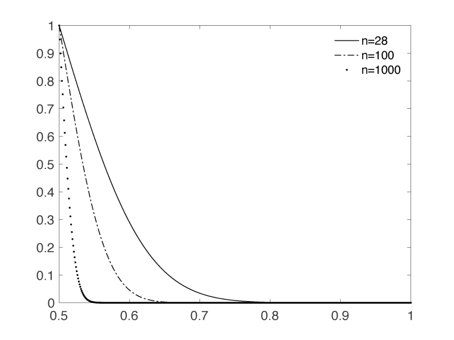
Press’s Q statistic is asymptotically distributed as $\chi^{2}$ with one degree of freedom. Figure 3 shows the plot of $p$-value of Press’s Q-statistic as a function of discriminant power. Larger discriminant power should correspond to smaller $p$-value. For instance, for $n=28$ subjects, the discriminant power of 0.85 can correspond to the extremely small $p$-value of 0.0002. Matlab code below is used to plot Figure 3.

n=28
for i=1:1000
    power(i) = i/1000;
    pval(i)=1-chi2cdf(n*(2*power(i)-1)^2,1);
end;
plot(power,pval);

To account for multiple comparisons, this small $p$-value needed to be corrected by computing the probability of the supremum distribution of a test statistic. However, this is not so trivial and requires the random field theory (Worlsey et al. 1995; Worsley et al. 1996). This is left as a future study.

The part of this study was supported by NIH grants NIH R01 EB022856 and R01 EB028753. We would like to thank Sterling C. Johnson of University of Wisconsin-Madison for providing the data used in Figure 1. We also like to thank Botao Wang of Xi’an Jiaotong University, China for pointing out the sign error in the original equation (8), which he corrected to be negative. The corresponding error in the MATLAB has been corrected.

References

- (1)
- Bishop (2006) Bishop, C. (2006), Pattern recognition and machine learning, springer.
- Chung et al. (2008) Chung, M., Kelley, D., Dalton, K. & Davidon, R. (2008), Quantifying cortical surface asymmetry via logistic discriminant analysis, in ‘IEEE Computer Society Conference on Computer Vision and Pattern Recognition Workshops’, pp. 1–8.
- Chung et al. (2005) Chung, M., Robbins, S., Dalton, K., Davidson, R., Alexander, A. & Evans, A. (2005), ‘Cortical thickness analysis in autism with heat kernel smoothing’, NeuroImage 25, 1256–1265.
- Flury (1997) Flury, B. (1997), A First Course in Multivariate Statistics, Springer.
- Hair et al. (1998) Hair, J., Tatham, R., Anderson, R. & Black, W. (1998), Multivariate Data Analysis, Prentice Hall, Inc.
- Hastie et al. (2003) Hastie, T., Tibshirani, R. & Friedman, J. (2003), The elements of statistical learning, Springer.
- Higdon et al. (2004) Higdon, R., Foster, N., Koeppe, R., DeCarli, C., Jagust, W., Clark, C., Barbas, N., Arnold, S., R.S. Turner, J. H. & Minoshima, S. (2004), ‘A comparison of classification methods for differentiating fronto-temporal dementia from alzheimer’s disease using FDG-PET imaging’, Stat Med 23, 315–326.
- Murphy (2012) Murphy, K. (2012), Machine learning: a probabilistic perspective, The MIT Press, Cambridge, MA.
- Shen et al. (2004) Shen, L., Ford, J., Makedon, F. & Saykin, A. (2004), ‘Surface-based approach for classification of 3d neuroanatomical structures’, Intelligent Data Analysis 8, 519–542.
- Subasi & Ercelebi (2005) Subasi, A. & Ercelebi, E. (2005), ‘Classification of EEG signals using neural network and logistic regression’, Computer methods and programs in biomedicine 78, 87–99.
- Thomaz et al. (2006) Thomaz, C., Boardman, J., Counsell, S., Hill, D., Hajnal, J., Edwards, A., Rutherford, M., Gillies, D. & Rueckert, D. (2006), A whole brain morphometric analysis of changes associated with preterm birth, in ‘SPIE Medical Imaging 2006: Image Processing’, Vol. 6144, pp. 1903–1910.
- Worlsey et al. (1995) Worlsey, K., Poline, J.-B., Vandal, A. & Friston, K. (1995), ‘Test for distributed, non-focal brain activations’, NeuroImage 2, 173–181.
- Worsley et al. (1996) Worsley, K., Marrett, S., Neelin, P., Vandal, A., Friston, K. & Evans, A. (1996), ‘A unified statistical approach for determining significant signals in images of cerebral activation’, Human Brain Mapping 4, 58–73.