Extracting the Possible Intrinsic Relation between Radiative Efficiency and Mass of QSOs: a Maximum Likelihood Method and its Application to the SDSS DR7 QSOs
Abstract
Radiative efficiencies of QSOs and its distribution encode rich information on the evolution of both masses and spins of massive black holes (MBHs) across cosmic time. In this paper, we develop a maximum likelihood method to statistically extract the intrinsic relation between radiative efficiency () and mass () of QSOs from their distribution on the luminosity-(empirically estimated virial) mass plane. By using mock samples, we find that strong constraint can be put on the relation at redshift from uniform QSO samples similar to those in Sloan Digital Sky Survey, and from QSO samples at (or ) if the magnitude limit of the survey can be (or ) magnitude deeper. Applying this method to the SDSS DR7 QSOs with , we find (or ) correlation for QSOs with the masses obtained according to the H (or Mg II) empirical mass estimator. These contradictory results may be due to the unknown systematic errors in the two mass estimators, preventing an accurate constraint on the relation by using current available QSO samples. We find that both the estimates of MBH mass and Eddington ratio distribution functions can be affected by the relation, suggesting that the determination of this relation is important for understanding the accretion and growth history of MBHs. In future, the intrinsic relation is expected to be strongly constrained by using QSO samples obtained from surveys deeper than SDSS if the host galaxy contamination and systematic errors of the mass estimator(s) can be well modeled or removed.
Subject headings
quasars: supermassive black holes–accretion, accretion discs–black hole physics–galaxies:activeI. Introduction
There is a consensus that massive black holes (MBHs; in the mass range ) lie in the centers of most galaxies. The mass growth and spin evolution of these MBHs are mainly governed by their accretion histories (Sołtan 1982; Yu & Tremaine 2002; Marconi et al. 2004; Yu & Lu 2004; King & Pringle 2006; Perego et al. 2009; Volonteri et al. 2013; Zhang, & Lu 2019, e.g.). Most QSOs are probably accreting gaseous material via the standard thin disk (Shakura & Sunyaev 1973; Novikov & Thorne 1973), and the mass growth rate of their central MBHs and the energy radiated from them are determined by the accretion rate and radiative efficiency, with the latter one directly determined by the MBH spin. MBHs with different masses are likely residing in different types of galaxies and environments, for example, MBHs at the high-mass end mostly reside in giant ellipticals, while those at the low-mass end mostly reside in spiral bulges, and thus they may have different accretion histories. A correlation between radiative efficiency (or spin ) and mass of active MBHs may emerge because of the environmental differences (Dotti et al. 2013; Dubois et al. 2014; Zhang, & Lu 2019, e.g., coherent or chaotic accretion). Such a correlation, if exists, may be a probe to the accretion histories of MBHs.
Currently, it is still not clear whether there is an intrinsic correlation or not. Davis & Laor 2011 directly estimated the radiative efficiencies for PG QSOs by , where is the bolometric luminosity, the rate inferred from the standard thin accretion disk modeling, and the speed of light. They found a correlation between the radiative efficiencies and MBH masses of those PG QSOs. Wu et al. 2013 further estimated the radiative efficiencies for SDSS QSOs and also found such a correlation, but they attributed it to an apparent correlation that is possibly induced by the sample flux limit and uncertainties in the MBH estimates (Raimundo et al. 2012, see also). Therefore, it is important to model and remove those effects induced by the sample selection and measurement errors in the relation analysis, in order to confirm whether there is an intrinsic correlation or not.
In the standard thin accretion disk model, the luminosity of a QSO at the optical-band depends on the accretion rate, MBH mass, as well as spin. For systems with a fixed Eddington ratio (e.g., ), the mass accretion rate decreases with increasing radiative efficiency, and the optical-band luminosity is correspondingly affected. To estimate the optical-band luminosities accurately, the relativistic correction is important if the spin (and correspondingly ) is large, and it is even substantial if because the peak of spectral energy distribution (SED) shifts to the optical-band and a larger corresponds to a higher peak. For these reasons, if there is an underlying intrinsic relation for a large sample of QSOs, their distribution on the luminosity-MBH (virial) mass plane may be significantly different from that of a sample without such an intrinsic relation.
In this paper, we develop a maximum likelihood method to extract the intrinsic relation, if any, from the distribution of a large number of QSOs on the luminosity-MBH (virial) mass plane, by utilizing the relativistic thin accretion disk model (Novikov & Thorne 1973, e.g.,). We take into account both the selection effects and the uncertainties in the MBH mass estimates. We first test the validity of this method by using mock samples of QSOs with different settings on the magnitude/flux limit, and then apply it to the SDSS DR7 QSO sample to obtain constraint on the possible intrinsic relation.
This paper is organized as follows. In Section II, we develop an analytical approach to calculate the optical band luminosity of individual QSOs by adopting the relativistic standard thin accretion disk model. Assuming such a model, we then introduce a maximum likelihood method in Section III for extracting the possible intrinsic relation. We generate a number of mock QSO samples and use the Markov Chain Monte-Carlo (MCMC) fitting technique to verify this method in Section IV. In Section V, we apply this method to the SDSS DR7 QSO sample and obtain constraints on the relation, MBH mass function (BHMF), and Eddington ratio distribution function (ERDF). Discussions and conclusions are given in Section VI and VII, respectively.
In this paper, we assume a flat CDM cosmology with parameters (, where km s-1 Mpc-3 with as the Hubble constant, and are the fractions of matter and cosmological constant in the local universe, respectively.
II. Relativistic thin accretion disk model: an analytical approach

In this section, we introduce an analytical model to estimate the optical luminosity radiated from a system that accretes material via the standard thin disk. This analytical method is calibrated by fitting to the numerical results obtained from the sophisticated relativistic accretion disk model implemented with the ray-tracing technique. Details for the ray-tracing method are provided in a previous work (Zhang et al. 2015, see). By adopting such a numerical method, we trace back each ray in a distant observer’s image plane to the accretion disk in the equatorial plane of the MBH. Below we show only the results obtained from the accretion disk models at the wavelength Å as it will be applied to the SDSS-like QSO surveys.
The optical luminosity of a QSO in the standard thin accretion disk model depends on the MBH mass , accretion rate (; or Eddington ratio ), efficiency (, or the MBH spin ), and the inclination angle (, defined as the angle between disk normal direction and line of sight). We adopt the ray-tracing method to obtain the observed luminosity at any frequency () by integrating over the surface of accretion disk
| (1) |
Here and are the two impact parameters describing the position of a disk element at (, on the observer’s sky. is the relativistic correction factor (Cunningham 1975, For more details see), where is the energy of a photon at the rest frame of the disk element and is the energy of the photon received by the observer. is the intensity at the rest frame of the disk element that emits the photon, which is given by
| (2) |
Here is the spectral hardening factor (Shimura & Takahara 1995; Salvesen et al. 2013), the intensity of a black body radiation at temperature , where
| (3) |
with the gravitational constant, the Thompson scattering cross section. The function , with (in unit of ), can be found in Gierliński et al. 2001.
For X-ray binaries, the typical value for the hardening factor is (Shimura & Takahara 1995). For QSOs, however, there are large uncertainties in the estimates of this parameter. For simplicity, we only consider the following two cases: (1) , corresponding to the most simple standard thin accretion disk model (Novikov & Thorne 1973), and (2) , considering the effect of Comptonization (Shimura & Takahara 1995). We find that the resulting luminosity from the latter case is almost the same as that predicted by the TLUSTY model (Hubeny & Lanz 1995) for a system with the same physical parameters (the differences in predicted luminosities usually dex).
The maximum likelihood method mentioned in Section III requires calculations of the (optical-band) luminosities of a large number of QSOs under various parameter settings. For a practical point of view, it may be more efficient if a fast and accurate analytical approximation to Equation (1) can be obtained for such an implementation.
For most QSOs, the optical-UV band luminosities given by Equation (1) follow a simple scaling relation, i.e., , when and the relativistic effects are ignored. Therefore, we introduce an analytical form to approximate the optical band luminosity for a wide range of conditions, i.e.,
| (4) |
Here is a correction factor by considering the relativistic effects and the bending of the black body radiation spectrum, and , is a constant and set to erg s-1 in order to make when .
Using the analytical Equation (4) to fit the numerical results obtained from Equation (1) at wavelength Å, we find that can be approximated described by
| (5) |
where , and . The value of and depend only on the spin parameter and . If assuming , we have
| (6) | ||||
If assuming , we have
| (7) | ||||
Here is the radius of the innermost stable circular orbit (ISCO) (Bardeen et al. 1972).
Figure 1 shows both the numerical results of as a function of and that given by the fitting formula (Eq. 5). The fitting formula well matches the numerical results with an error dex. In most conditions, , and thus . However, for QSOs with , i.e., if the MBH mass is large and the Eddington ratio is small, e.g., and , the correction factor can be much smaller, i.e., . is also sensitive to the values of spin and if .
According to Equation (4), we have . Thus, if the correction factor is close to unity, for any given , and , if varying from to , the optical-UV luminosity can be reduced by dex. For QSOs with MBHs at the high-mass end or small Eddington ratio, becomes also significant. Therefore, the optical-UV luminosity depends significantly on the radiative efficiencies. For individual QSOs, there is a degeneracy between the unknown and , as suggested by Equation (4), which prevents the determination of simply from observations on and . However, it may be done for a large sample of QSOs, as the joint distribution of the MBH masses and optical-UV-band luminosities depends on the underlying intrinsic correlations between MBH mass and radiative efficiency . The details of our method is shown in the following sections.
III. A maximum likelihood method
In this section, we introduce a maximum likelihood method that can be used to extract the possible intrinsic relation. We start with a general formalism of the method in Section III.1, and then consider more specific selection function(s) and probability distribution function (PDFs) of various QSO properties in Section III.2 and III.3, respectively.
III.1. The likelihood function
We denote the joint PDF of QSOs as , which describes the number density of QSOs with luminosity in the range from to , true MBH mass in the range from to , and redshift in the range from to . For most QSOs, and can be directly measured with high accuracy. However, the observational determined MBH mass may substantially deviate from the true MBH mass and this deviation may be denoted by a PDF . Therefore, the observational determined joint PDF of QSOs, , is given by
| (8) |
Assuming that the selection of QSOs depends only on the flux/luminosity limit of a QSO survey, and the selection function can then be denoted by . Note that this assumption may be a good approximation for the SDSS QSO survey, however, it may be an oversimplification for QSO surveys in general. In order to extract the intrinsic joint PDF, we define a likelihood function as (Marshall et al. 1983, see)11 1 In some cases, as the input parameters of the model poorly describe the observed (or mock) samples. For example, the scatter of the observational determined MBH masses around the true MBH masses given by Eq. (14) below is set too small to explain the observed mass distribution of QSOs. For these cases we set to be a tiny value to avoid odd results.
| (9) | ||||
where is the total number of QSOs in the observational sample. The first term in the right side of Equation (9) sums over all the observed QSOs giving their individual masses , luminosity , and redshift , and the second term integrates over , , and . It is practically convenient to use the joint distribution of MBH and Eddington ratio, i.e., rather than in modeling the intrinsic distribution of QSOs. According to Equation (4), the joint PDF can be also described as
| (10) |
We can then calculate Equation (9) according to the assumed joint distribution of and the intrinsic relation.
III.2. Observational bias and selection functions
For a given emission line, assuming that the true mass of the MBH can be estimated by an ideal empirical relation22 2 We assume that the mass estimator is a function of , which is used for the selection in Equation (9). Usually, the mass estimator is a function of the continuum luminosity around the emission line , which may be different from (at ). Considering that the continuum spectrum of a QSO can be described by a power law, can always be obtained according to a given , and the difference between these two luminosities is then a constant that can be absorbed into the parameter . , e.g.,
| (11) |
where , and are constants, FWHM is the full width at the half maximum of the adopted emission line. Due to various observational uncertainties, the empirical mass estimator may be not accurately obtained, so that it is scattered around, or biased from the true ones (Shen 2013, e.g., due to stochastic dispersions in luminosity, see). As a result, the observed mass of QSOs given by the empirical mass estimator for QSOs now becomes
| (12) |
where is a random deviation following a Gaussian distribution with a zero mean and a scatter of .
In this paper, the adopted mass estimator is based on either the H or MgII line, thus, following Shen et al. 2011 we set , assuming that both of these two emission lines are coming from the same regions of the broad line region (BLR; see Onken & Kollmeier 2008 for details.). Under such assumption, we have ignored the complexities of any systematic errors dependent on FWHM. 33 3 However, we notice that observations do suggest that may be biased and not exactly (Wang et al. 2009, e.g.,). For the possible systematic errors of FWHM and its impact on our results, see discussions in Section V.3. Then the observed MBH masses will be biased from the true ones by the systematic that is not well probed by the empirical estimator, i.e.,
| (13) | ||||
where describes the possible systematic error in the MBH mass estimator with a dependence on the QSO luminosity showing by the parameter (similar to the parameter in Shen 2013 and Shen & Kelly 2012), and is a characteristic luminosity.
To cover such complexities, we assume that the PDF of the observational determined MBH masses () around the true MBH mass () is described by a Gaussian function
| (14) | ||||
Here we set erg s, which is the QSO luminosity when , and .
We also assume that the selection function is simply given by
| (15) |
for a flux limit QSO survey. Here is the fraction of sky coverage of the survey, and is the luminosity limit determined by the flux limit of the survey. For QSOs in SDSS Data Release 7, the effective sky coverage is about deg2 (Shen et al. 2011) and thus if the luminosity of a QSO at wavelength Å is larger than the luminosity limit . The fraction of QSOs with mass measurements in these spectroscopically targeted samples is close to unity, thus it can be safely ignored (Schulze et al. 2015, see discussions in). The at redshift for a given flux limit of the SDSS survey can be found in Richards et al. 2006.
III.3. The distribution functions of the intrinsic QSO properties

We assume that the intrinsic PDF of and for QSOs within a sufficiently small redshift bin ( to ) can be approximated as
| (16) |
where represents the redshift evolution of the normalization and represents the joint distribution of MBH mass and Eddington ratio. For simplicity, we assume
| (17) |
where and are two free parameters. Below we fix simply because it is close to the middle of the redshift range that is considered in this paper.
We further set
| (18) |
where is described by a Schechter-like function 44 4 We have also try an alternative double power-law model: However, our following calculations show that there is no clear difference between the results obtained by adopting these two different distribution forms. In the rest of the paper we discuss only the results from the Schechter-like function.
| (19) |
where , , , and are all free parameters.
The conditional Eddington ratio distribution for QSOs with the same is assumed to be described by
| (20) | ||||
or alternative a Gaussian function
| (21) |
where
| (22) |
, , and are all free parameters.
We assume that the intrinsic relation is simply described by
| (23) |
where and are two free parameters, . The MBH spin is in the range from to , and correspondingly is confined in the range from to in the standard thin disk accretion model. In the model, the inclination angle for each QSO is fixed at .
IV. Mock sample test of the method
In this section, we generate mock QSO samples by setting different sets of the model parameters and illustrate how the observed PDFs are affected by the assumed relation. We further use the maximum likelihood method described in Section III to check how well the relation can be reconstructed from the mock observations, or how it is biased due to a number of complexities (e.g., the host galaxy contamination, or scatterings in the inclinations). The details are described in the following sections.
IV.1. Mock QSOs

Here we introduce the initial conditions and detailed implementations for the mock sample generation. If not otherwise stated, these conditions and implementations are also used for Section IV.2, IV.3, IV.4. We assume , , , , , , , and , such that they are close to the fitting results from Schulze et al. 2015 for SDSS QSOs at . Then the joint PDF can be obtained from Equations (17)-(20). Given the above initial conditions, the total number of the intrinsic samples can be obtained by
| (24) |
We generate a number of mock QSOs by the Monte-Calro method. For simplicity, we also assume and , if not otherwise stated. The radiative efficiency of each mock QSO is given by Equation (23), by assuming and adopts a value in between and . Then the optical band luminosity at Å of each mock QSO is estimated according to Equation (4).
We find that the constraint on the intrinsic relation weakly depend on the sample size or correspondingly for a given magnitude limit. Therefore, we simply assume that . We assume that a QSO at redshift is “observable” if its , and then the “observed” mass of this mock QSO is set according to Equation (14) by assuming , and . Finally, we obtain a sample of mock QSOs with “observational” properties of , , and , . According to such a mock sample, we can then use the maximum likelihood in Equation (9) to recover the input parameters, and check how well can they be reproduced.
Figure 2 shows the distributions of mock QSOs on the plane resulting from the same but two different relation, one with (blue contours) and the other with (red contours). These two distributions are quite different, suggesting that the apparent joint distribution depend not only on but also on the intrinsic correlation, if any. Due to such differences, the intrinsic relation can be extracted from the 2D distribution of QSOs on the luminosity versus observed MBH mass plane.
IV.2. Effects of the flux limit of the QSO survey


The distribution of QSOs from a survey on the plane only shows those QSOs above the magnitude/flux limit of the survey (see Figure 2). Therefore, the constraints on the relation obtained from such a distribution may strongly depend on the flux/magnitude limit of the survey.
To investigate how the constraints on the model parameters depend on the flux limit, we perform a number of Monte Carlo Markov Chain (MCMC) calculations. We consider three cases, i.e., is assumed to be , , and , respectively. For each of these cases, we first generate mock QSO samples at the redshift bin 55 5 It can be similarly done for any other redshift bins. and the -band magnitude limit is set to be mag (similar to the SDSS QSO survey), , , or mag. Then we use the MCMC method to recover the input values of those model parameters by adopting the likelihood function given by Equation (9). The model considered here contains parameters (with and ), or a model with parameters by only fixing , so that we can see the effects of constant mass bias by comparing these two models.
To show more clearly the constraints of the intrinsic relation, we obtain the two dimensional (2D) confidence level for the reconstructed relation according to the accepted values of and in each chain of the MCMC fittings. The results for the case are shown in Figure 3. We can see that the input relation can be well recovered when the flux limit is sufficiently low, i.e., mag. Note that the best-fit values of and slightly deviate from the input ones when , which is simply due to the random noises introduced by the Monte Carlo method in generating the mock QSO samples.
When mag, there is a strong degeneracy between and (top panel of Fig. 3) and the relation cannot be well constrained (bottom panel of Fig. 3). Such a degeneracy is expected as low mass QSOs can not be observed, and the observed sample covers only a small range of . If these faint QSOs can be included in the sample, as illustrated in Figure 3 when mag, the degeneracy will then be almost disappeared.
Figure 4 shows the constraints on relation for cases with different input values for by using either the or parameter model. We can see that, in most cases, the constraints on both and are significantly improved if the magnitude limit of the QSO survey increases to mag. Note here that the value of is always poorly constrained (see bottom panel of Fig. 4) if there is no intrinsic relation (i.e., ) and if the is included in the MCMC fitting. As reflects the systematic errors in the mass estimates, is strongly degenerate with when . However, such a degeneracy can be breakup when is significantly different from .
We find that the constraints on the intrinsic relation depend also on the initial value of . If , the QSOs in the mock samples are statistically brighter than those if (See Fig. 2), thus the constraints are slightly stronger (See Figure 4). For other parameters in the model, we also find that they can be reproduced with considerable accuracy.
Similar constraints on the intrinsic relation can be also obtained for mock samples at other redshift bins if assuming that the intrinsic distribution function depends weakly on the redshift. According to the relation between the luminosity and the -band magnitude limit given by Richards et al. 2006, mag at corresponds to and this luminosity range corresponds to mag at . Therefore, it is possible to get a reasonably constraints by using the SDSS QSO sample at redshift as its magnitude limit is mag. Similarly, if a QSO survey can have the magnitude limit of mag, then it would provide strong constraints on the relation at redshift .
IV.3. Scattering of and

For the mock simulations in the previous section, we have set and assume that the relation is explicitly given by Equation (23). In reality, however, it is likely that is randomly distributed over a range of values, and the relation may have some scatters. To check whether the maximum likelihood method can still work well under these circumstances, we generate a group of mock samples with settings similar to those in Section IV.1 except uniformly distributed between and a Gaussian scatter of dex on the given by Equation (23). We generate mock QSO samples at and set mag to mimic the case of SDSS DR7 QSOs. We then use the MCMC fitting technique to obtain constraints on the relation.
Figure 5 shows the results of the constraints on the intrinsic relation. The green dots show the exemplified value of for the ‘observed’ sample. The blue solid line represents the best-fit value and the region enclosed by the gray shadows shows the constraints. It can be seen that the relation can still be well reproduced, even if there are some scatters in the radiative efficiencies. As demonstrated in Section IV.2, the constraints on the intrinsic correlations is stronger for the samples with than those with .
If the scatter is large, then Equation (23) is not so meaningful and the reconstructed value of will then likely be zero, which may only reflect an effective intrinsic relation. We find that the other model parameters, defining the form of , can also be well reconstructed within confidence level. Therefore, we conclude that the maximum likelihood method introduced in this paper can work well even if there is a large scatter in the relation. Note here that there might be a scatter for the intrinsic relation, if any, which is not considered above. In principle, one may add more model parameters to include such a possiblity for the relation when considering the likelihood function. However, the calculations will be more complicated and computationally heavy66 6 The scatterings of can be described by a probability function similar to that shown in Equations (20) and (21), then the mass-luminosity joint distribution is given by where is given by Equation (4). Then the likelihood function of Equation (9) can be accordingly modified (by using the integrals of the above equation) and calculated. . In this paper, we do not intend to introduce such model parameters.
IV.4. Effect of host galaxy contamination
The contamination from host galaxies makes some of those QSOs with intrinsical luminosities below the magnitude limit become observable, and thus leads to a modification of the distribution of those QSOs on the observed plane. Therefore, the recovered intrinsic relation may be biased if the host galaxy contamination is not well modeled for the QSO sample(s).
Here we use MCMC simulations to investigate how the constraints of the intrinsic correlations are effected by the uncorrected host galaxy contamination. For the demonstration purpose, here we consider two different models for host contamination. The first one is from Shen et al. 2011, in which the ratio of host to QSO luminosity at a given QSO luminosity is given by77 7 Note that this correction is for the Å luminosity. However, we adopt it here only to illustrate the importance of the host galaxy contamination. The correction in Shen et al. 2011 is a function of the total luminosity (see Eq. (27)), which is not initially known for the mock QSOs, thus, we need to convert it as a function of intrinsic QSO luminosity by refitting to the original equation.
| (25) |
where , and . Another one is derived from Schulze et al. 2015(See their Fig. 2):
| (26) |
and . The upper limits of for the above two equation are obtained by setting the host to QSO luminosity ratio to zero. For QSOs with luminosities larger than the upper limit, the host contamination is negligible. Figure 6 shows the ratio of host to QSO luminosity given by these two models.
We generate a group of samples similar to those in Section IV.1 but at lower redshift (such that the host galaxy contamination becomes more important). Initially we set (or ). We then add the luminosity of galaxies into the samples according to Equation (25) or (26). For each group of samples we use MCMC simulations (of which the host galaxy contamination is not included), to investigate whether the correlations can be correctly recovered.
The results are as follows. we found that if the host galaxy contamination is similar to Shen et al. 2011, the recovered will be biased to higher values. For example, the recovered is (or ) if the intrinsic (or ). However, if the contamination is similar to that given by Schulze et al. 2015, the effect of host galaxy contamination is not important. Both the intrinsic relation and other model parameters can be well recovered.
These results suggest that whether the intrinsic relation can be well recovered or not depends on the exact form of the host galaxy contamination. For example, the host galaxy contamination from Shen et al. 2011 is more severe than those in Schulze et al. 2015 for faint QSOs (See in Figure 6). The distribution of the observed samples are more significantly modified, resulting in a strong bias of the intrinsic correlations. The above results suggests that, for a comprehensive study, it is important to investigate the effects of host galaxy contamination in the recovery of correlations, especially for low redshift QSO samples.
V. Application to the SDSS DR7 QSO samples
| Name | fixed parameters | Host Galaxy correction | BHMF | ERDF | |
|---|---|---|---|---|---|
| M11N2S | None | Schechter | Schechter | ||
| M12N2S | None | Schechter | Schechter | ||
| M12N1S | None | Schechter | Schechter | ||
| M12S2S | Shen11 | Schechter | Schechter | ||
| M12U2S | Schulze15 | Schechter | Schechter | ||
| M13N2S | None | None | Schechter | Schechter | |
| M11N2SG | None | Schechter | Gaussian | ||
| M13N2SG | None | None | Schechter | Gaussian |
| Model | z=0.34-0.5(H) | z=0.5-0.7(H) | z=0.5-0.7(MgII) | z=0.7-0.9(MgII) | |||||||
|---|---|---|---|---|---|---|---|---|---|---|---|
| M11N2S | |||||||||||
| M12N2S | |||||||||||
| M12N1S | |||||||||||
| M12S2S | |||||||||||
| M12U2S | |||||||||||
| M13N2S | |||||||||||
| M11N2SG | |||||||||||
| M13N2SG | |||||||||||
In this section, we apply our maximum likelihood method to the SDSS QSOs samples to extract the underlying intrinsic correlations. We apply our method to fit the QSOs in each redshift bins by varies different assumptions on the model (See Table 1). The details are in the following Sections.
V.1. SDSS QSOs samples
In this section, we briefly describe the SDSS QSO samples (Shen et al. 2011). In the catalogue of SDSS QSOs [Data Release 7 (DR7)], QSOs have -band magnitude , at least one broad emission line broader than , and the estimations of central MBH masses. About half of these SDSS QSOs (total ) QSO at were selected out to form a homogeneous, statistical sample, which is primarily a flux limited sample with -band magnitude at , at and an additional bright limit of . We select the QSOs with in this sample (total number ) to form our SDSS QSO samples. Among them, those QSOs with mass estimation errors dex were removed from the QSO sample. The total number of these QSOs is only of the whole sample, thus the removal of them only slightly affects the overall completeness.
We have shown in Section IV.2 that the SDSS-like QSO samples beyond are unlikely set useful constraints on the intrinsic correlations, thus we do not include the QSO samples with . Also, we notice that the completeness of the QSO samples at are almost unity (Richards et al. 2006), which greatly simplify our maximum likelihood method. The luminosity at Å is converted from , the K-corrected -band absolute magnitude (Richards et al. 2006).
We divide those QSOs with into three redshift bins, i.e., , , and . For QSOs with , their masses can be obtained by utilizing the H estimator, while for those with , their masses can be obtained by utilizing the MgII estimator. For the redshift bin , QSO masses can be obtained by using either the H or MgII estimator. Therefore, a comparison between the results obtained by utilizing the H estimator and those by the MgII estimator in this bin may provide an estimation of the effects induced by possible systematical errors in different mass estimators. The total numbers of QSOs using the H estimator are and in the bins and , respectively, while those using the MgII estimator are and in the bins and , respectively. Figure 9 shows the two dimensional number distribution of these QSOs in the plane.
V.2. Models


The MCMC fitting results of the SDSS QSOs samples may depend on the details of the modeling. For example, the choices of essential model parameters, forms of BHMF, correction of the host galaxy contamination, and , may all affect the fitting results. To explore their possible impacts, here we adopt eight different models, with the underlying assumptions of each model listed in Table 1.
All models ignore the host galaxy contamination, expect model M12S2S and M12U2S, of which we have assumed that the host galaxy correction is given by Shen et al. 2011 and Schulze et al. 2015, respectively. According to Shen et al. 2011, this ratio is given by
| (27) |
where , and ; while according to Schulze et al. 2015, it is given by
| (28) |
where .
The above two fitting formulas are valid only when (Shen et al. 2011) and , respectively. By adopting these corrections, we can recover the intrinsic QSO luminosity, and use the MCMC model to extract the intrinsic correlations from these samples.
V.3. The intrinsic relation

The intrinsic relation is assumed to be a power-law with slope and normalization at (see Eq. 23). The best fits of these two parameters obtained from different models are summarized in Table 2 and shown also in Figure 7. Since the constraints on is generally weak, it is more clear to see the confidence level of the intrinsic relation in the plane, which is shown in Figure 8.
For the QSO samples utilizing the H mass estimator, we summarize our main results at as following. As shown in Table 2, the most likely value of is obtained from the QSO sample with redshift by using different models, and it is still positive but slightly smaller () from the QSO sample with . The most likely values of are obtained from the QSO samples with . Apparently, most models suggest a positive correlation between and , i.e., the larger the MBH mass, the higher (or spin). As also seen from Figure 8, the constraint on the relation is quite tight when it is obtained from the QSO sample with (panels in the first and fourth columns), while it has larger uncertainty when obtained from the QSO sample with . For all models, is low at and becomes high with at .
For the QSO samples utilizing the MgII mass estimator, we summarize the main results at as following. The best-fit values of and . Most of those models tend to result in a negative correlation, though only four among the eight models have at confidence level. The constraints on the relation shown in Figure 8 clearly suggest that is large when and small when . For most models, the obtained results are inconsistent (at level) with those constraints obtained from the QSO sample in the same redshift bin but utilizing the H mass estimator. Note that models like M13N2S, M11N2SG or M13N2SG have very weak constraints on the correlations, thus it seems that they can still be consistent with those utilizing the H mass estimator.
As seen from Figure 8 (the third and sixth column panels), almost all models for the QSO sample with result in a constraint on relation with which the contour covers almost the entire parameter space. Thus, and cannot be well constrained if , as expected and predicted in Section IV.2 for SDSS QSOs at such redshift range or higher redshifts.
Figure 9 shows the comparison between the best-fits obtained from model M12S2S (as examples) and observational distributions of QSOs in the plane. We can see that they are well consistent with each other (The observational distributions can also be well fit by other models in Table 1). The joint distribution obtained by using the MgII estimator is clearly narrower in mass direction (top right panel of Fig. 9) than that using the H estimator (bottom left panel of Fig. 9). Such a difference is similar to that between the cases with and shown in Figure 2. This explains why we always get the most likelihood value of positive for the QSO sample using the H estimator but a negative for those samples using the MgII estimator.
V.4. The bias due to the mass estimators, host galaxy contamination and other parameters in the model
If inconsistencies between the results from H and Mg II mass estimator are due to the bias of luminosity, then including should make their fitting results consistent with each other. However, we do not see such consistency within confidence level for those models including (e.g., M13N2S, M13N2SG), but we see larger uncertainties in the recovered correlation. Such inconsistency are also not disappeared by including a constant as a free parameter or not in the MCMC simulations, although is usually non-zero (, see Fig. 12) resulting from all these models.
We find that our above conclusions on the relation for SDSS QSOs are not affected much by including host galaxy contamination or not in the model. This is possibly because the complexities of host galaxy contamination functions. For example, the adopted two kinds of host galaxy contamination may be either overestimated or underestimated. On the other hand, the host contamination may vary from galaxy to galaxy, the simple functional correction shown in Equations (27) and (28) may be not accurate enough.
We also find that our conclusions on correlation does not affected by changing to , or adopting a different distribution function of (e.g., using Equation 21 rather than Equation 20) in the modeling. For all the eight models listed in Table 1, we have also try other variations of them, e.g., changing the form of the Equation 19 in model M13N2S to double power law model (See its footnote); or make host galaxy correction by Equation 27 in addition to model M13N2S, we do not see significant differences in the recovered correlations. These results suggest that the inconsistencies are not due to these complexities. Note that only a few cases were test here and the above conclusion may need further confirmation by using a more sophisticated model, and etc, in the future.
Thus, the inconsistency between the constraints on relation obtained by using the H estimator and that using the MgII one may be partly due to the possible bias induced by using FWHM in the same way for H and MgII in the estimator. It is commonly assumed that the MgII and H emitting regions are the same and have the same line-width (Onken & Kollmeier 2008; Salviander et al. 2007, e.g.,). In the SDSSs sample we adopted, they use a fix ratio of for FWHM in both the H and MgII estimators (Shen et al. 2011). However, observations suggest that it can be different from , as they may be from different line-emitting locations in the BLR (Wang et al. 2009, e.g.,). Currently, it is still unclear whether the estimates of base on MgII consistent with those of based on H. In the current work, we cannot include FWHM in our modeling, thus, if there is some systematics in the FWHM, we cannot reduce them here.
V.5. Constraints of BHMF and ERDF

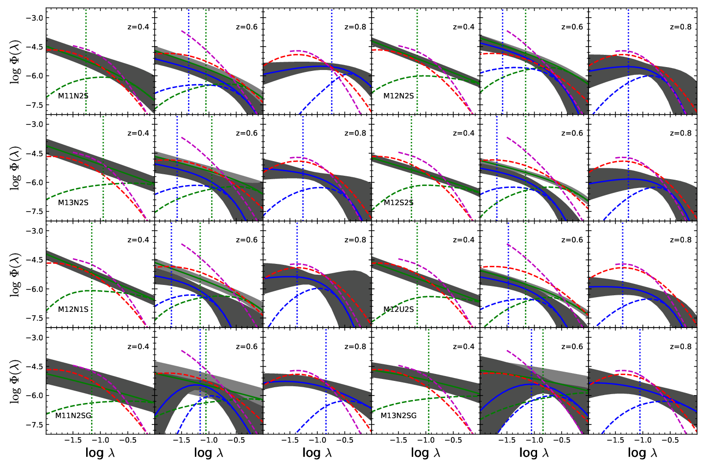
In addition to the constraint on the relation, even strong constraints on the BHMF and ERDF at redshift can be also obtained from our model. The marginalized intrinsic BHMF and ERDF of the QSOs in each redshift bin are given by
| (29) |
and
| (30) |
respectively.
Due to the flux limit, only those QSOs above the luminosity limits can be observed. The observed marginalized intrinsic BHMF and ERDF of the QSOs in each redshift bin is given by
| (31) |
and
| (32) |
respectively. Note that the results of and depend strongly on the lower limit of the integration of , especially if is small. It may be not so meaningful to consider the ERDF for MBHs with mass substantially below , as the completeness of drops rapidly below (see Fig. 10). To exclude the parameter ranges where the QSO samples are highly incomplete, we set the lower limit of for the integrations in above Equations (30) and (32), below which the completeness of , i.e., , . This lower limit is when , when , and in redshift .
Figure 10 shows the BHMFs at different redshift obtained from all the eight models listed in Table 1. As seen from this Figure, the resulting BHMFs are slightly model dependent for QSOs at , and some of them are significantly different from those given by Shen & Kelly 2012 and Kelly & Shen 2013. This may suggest that, including the relation and the systematic errors in the estimated MBH masses in the model can affect the determination of BHMFs (similarly the ERDFs, see below). We find that, the larger the slope of the relation, the larger the difference between the resulting BHMF and that given by Shen & Kelly 2012 and Kelly & Shen 2013. For example, the models M11N2SG and M13N2SG result in small value of , and the resulting BHMFs are very close to those given by Shen & Kelly 2012 and Kelly & Shen 2013. For other models, the difference are more apparent as the of them is larger.
Figure 11 shows the ERDFs in different redshift bins obtained from our models. As seen from this Figure, the resulting ERDFs are also slightly model dependent. In the redshift bin , the ERDFs obtained from our models have a relatively shallower slope than and do not drop rapidly around as those in Shen & Kelly 2012 and Kelly & Shen 2013. This is partly because we set a boundary for the Eddington ratio at , and partly because of the positive correlations. Similar results for ERDFs are also obtained from the QSO sample with utilizing the H mass estimator. For the QSO sample with utilizing the MgII mass estimator, the resulting ERDFs drop rapidly near , and negative (rather than positive) correlations are obtained from different models. These results again suggest that a none-zero correlation can affect the constraints on ERDF as well as BHMF and raise the importance of considering the relation.
In the redshift bin , both the BHMFs and ERDFs resulting from the fittings by utilizing the H (lines in green) and MgII (lines in blue) mass estimators have some discrepancies. Such discrepancies are likely due to the fact that the H and MgII mass estimators are not well modeled. As all parameters describing the BHMF, ERDF, and the relation are set free in the MCMC fittings, a biased modeling of the mass estimator will then result in biased relation (as shown in Section V.4), BHMF and ERDF. In the future, we expect that such discrepancies may disappear if we have more better modeling of the mass estimators.
Note that the way to obtain in our method is very different from those in Kelly & Shen 2013 and Schulze et al. 2015. The Eddington ratio is derived directly from the optical luminosity and the mass of QSOs in Kelly & Shen 2013 and Schulze et al. 2015, i.e., as they adopt the empirical bolometric correction to directly get the total luminosity. In their methods, the Eddington ratio can be obtained for each sample object. In our method, of each object cannot be separately obtained from observations and of each individual object is unknown. In addition, in our method , is also different from those adopted in Kelly & Shen 2013 and Schulze et al. 2015, according to Equation (4).
We notice that Shen & Kelly 2012 and Kelly & Shen 2013 adopts different modeling between the MBH and luminosity, and their constraints on ERDF is significantly different from each other, especially at high Eddington ratio end. In our model, the Eddington ratio is generally complete if for the QSOs at redshift . Note that this completeness is for only the samples that the completeness of the black hole masses are also larger than .
V.6. Fitting results of other parameters

The maximum likelihood method applied here can put constraints on not only the intrinsic relation, BHMF, and ERDF, but also simultaneously the other parameters in the model, e.g., such as the parameters related to the mass estimators. Figure 12 shows that our best-fit mass scatter for QSOs with is around dex, consistent with the value dex that commonly used in the literature (Schulze et al. 2015; Kelly et al. 2010, e.g.,).
According to those models with -parameters, we find that the constant mass bias and the possible luminosity-dependent systematic errors introduced by in the H and MgII estimators may be different. For the QSO sample with , all models result in , by using the H estimator, while for the QSO sample with , they result in , by using the MgII estimator. These results suggest that both the constant mass bias and the luminosity-dependent systematic error in the MgII estimator may be different with those in the H one.
VI. discussions
Due to the discrepancies between results obtained by using the Mg II and H mass estimators, it is difficult to put solid conclusions on the relation, the BHMF and ERDF of the SDSS QSOs. If both of the two mass esimators are well-modeled, we expect that these results should be consistent with each other. If not, both the relation and the BHMF or ERDF would depend on the correctness of mass estimators, and they will be biased if there are any remaining systematics. Such unknown systematics could possibly be addressed in the future, by extending our models to include FWHM, velocity dispersion, or other details of the mass estimator(s) [similar to some previous works, e.g.,][](Kelly et al. 2009). On the other hand, it should be straightforward to expending our model likelihood function (Eq. 9) to fit QSOs samples with masses from two different mass estimators with equal weight. However, the accuracy of such a model is unknown, as currently we do not known whether the relations obtained by using the MgII and H mass estimators are biased to negative or positive values. Only in the cases that the MgII and H mass estimators are biased in opposite ways we can get more accurate results. Thus, this problem may be solved if the uncertainties in the Mg II and Hbeta mass estimators can be well determined or a better mass estimator can be provided, in which case more robust and consistent constraints on the relation can be obtained.
The relation of QSOs has also been investigated and discussed in some preivous works but in a way different from the maximum likelihood method introduced in this paper. In these works, the radiation efficiency of individual QSOs were mostly estimated according to the QSO bolometric luminosities and the inferred accrection rates (Davis & Laor 2011; Wu et al. 2013; Raimundo et al. 2012; Trakhtenbrot et al. 2017; Schulze et al. 2017; Shankar et al. 2019, e.g.,). However, the selection effects of the flux limits of QSO surveys must be carefully considered, as it may lead to an apparent correlation between and , even if there is no intrinsic one (Wu et al. 2013; Raimundo et al. 2012, e.g., see). Furthermore, the model adopted in these works is not physical and self-consistent, as the averaged bolometric correction is used for those QSOs with the same luminosity at a given band but different masses and accretion rates. According to the accretion disk model, the bolometric corrections for QSOs should be dependent on the masses, spin, and accretion rate (Netzer & Trakhtenbrot 2014, see more discussions in). As a comparison, our work is a statistical method, in which we do not focus on individual QSOs but the statistical distributions of QSO samples on the mass-luminosity plane. In our method, we have also taken account of the complexities due to the selection functions and the biases in the mass estimators, which is self-consistent as demonstrated by using the mock data.
The correlation may be also inferred from the (cosmological) evolution of black hole spins and mean radiative efficiencies (Li et al. 2015; Zhang, & Lu 2019, e.g.,). The cosmological growth of the QSO masses and total luminosity radiated from QSOs are directly linked by the (mean) radiative efficiency, and thus the radiative efficiency (or spin) can be constrained according to the cosmological evolution of black hole mass density and the total radiated energy inferred from the QSO luminosity functions [see the Sołtan argument in Sołtan 1982 and the extended one in Yu & Lu 2004; the possible evidence for cosmological evolution and mass dependent of radiative efficiency in Li et al. 2015; Wang et al. 2009]. However, the results on the relation possibly obtained by using the above method suffer from the large uncertainties in the empirical relations between black hole mass and galaxy properties that are adopted to estimate black hole mass densities and the uncertainties in the bolometric corrections and the luminosity functions used to estimate the QSO total energy densities. Considering also that our current model does not include the detailed physics to trace the cosmological black hole growth, spin and radiative efficiency evolution, it would be important to cross check future results on the relation obtained from the method presented in the current paper with those from that mentioned above.
VII. Conclusions
The intrinsic relation between radiative efficiency () and mass of MBHs () in QSOs, if any, is important for understanding the MBH/QSO cosmological evolutions. In this paper, we develop a maximum likelihood method to extract the intrinsic relation from the distribution of QSOs in the optical luminosity-MBH mass plane. We adopt a simple relativistic thin accretion disk model to estimate the radiation of QSOs in the optical-UV band.
We first use mock QSO samples to demonstrate that the intrinsic relation, if any, can be extracted from a SDSS-DR7-like QSO sample with . For QSOs at higher redshift with , the intrinsic relation can be robustly extracted only if a QSO survey can go about magnitude ( mag) fainter than the current SDSS survey. If a SDSS-like survey with flux limit down to mag, then it is possible to identify the intrinsic relation for a QSO sample at redshift upto .
We find that such an intrinsic relation can still be extracted even if it has a scatter. Under some circumstances, if the samples are contaminated by host galaxy and it is not corrected, the recovered relation may be significantly biased from the intrinsic ones.
We apply our method to the SDSS QSOs in the redshift range and adopt a number of models to perform MCMC simulations and get constraints on the intrinsic relation. We find signs of positive correlations () for QSOs at utilizing the H mass estimator. However, for QSOs at utilizing the Mg II mass estimator, we find that the correlations become negative (). This inconsistency is likely due to the unknown different systematic errors in these two mass estimators, but not due to the host galaxy contamination.
We also derive constraints on the BHMF and ERDF of QSOs. Although our results are broadly consistent with some previous studies, e.g., Shen & Kelly 2012 and Kelly & Shen 2013, we find that the relation, if does exist, can affect the determination of BHMF and ERDF significantly; This may suggest that, to obtain precise constraints on both the BHMF and ERDF, it is necessary to include the relation in the modeling.
We conclude here that the maximum likelihood method introduced in this paper can set robust constraints on the intrinsic relation, if any. However, if there are some unknown systematic errors in the mass estimators that cannot be well modeled, the recovered relation may be strongly biased from the true one. We expect that the understanding of the systematics on the MBH mass estimator(s) will be improved a lot and the QSO surveys will go much deeper than the SDSS QSO survey adopted here, which will enable the revealing of the intrinsic relation and better determinations of the BHMF and the ERDF of QSOs. In addition, it is possible to solve this problem if we can improve our model to consider the complexities of the FWHM of the mass estimators.
References
- Bardeen et al. (1972) Bardeen, J. M., Press, W. H., & Teukolsky, S. A. 1972, ApJ, 178, 347
- Bentz et al. (2009) Bentz, M. C., Peterson, B. M., Netzer, H., Pogge, R. W., & Vestergaard, M. 2009, ApJ, 697, 160
- Cunningham (1975) Cunningham, C. T. 1975, ApJ, 202, 788
- Dauser et al. (2010) Dauser, T., Wilms, J., Reynolds, C. S., & Brenneman, L. W. 2010, MNRAS, 409, 1534
- Davis & Laor (2011) Davis, S. W., Laor, A., 2011, ApJ, 728, 98
- Dotti et al. (2013) Dotti, M., Colpi, M., Pallini, S., Perego, A., & Volonteri, M. 2013, ApJ, 762, 68
- Dubois et al. (2014) Dubois, Y., Volonteri, M., & Silk, J. 2014, MNRAS, 440, 1590
- Gavignaud et al. (2008) Gavignaud, I., Wisotzki, L., Bongiorno, A., et al. 2008, A&A, 492, 637
- Gierliński et al. (2001) Gierliński, M., Maciołek-Niedźwiecki, A., & Ebisawa, K. 2001, MNRAS, 325, 1253
- Hubeny & Lanz (1995) Hubeny, I., & Lanz, T. 1995, ApJ, 439, 875
- Kelly et al. (2009) Kelly, B. C., Vestergaard, M., & Fan, X. 2009, ApJ, 692, 1388
- Kelly et al. (2010) Kelly, B. C., Vestergaard, M., Fan, X., et al. 2010, ApJ, 719, 1315
- Kelly & Shen (2013) Kelly, B. C., & Shen, Y. 2013, ApJ, 764, 45
- King & Pringle (2006) King, A. R., & Pringle, J. E. 2006, MNRAS, 373, L90
- Kochanek et al. (2012) Kochanek, C. S., Eisenstein, D. J., Cool, R. J., et al. 2012, ApJS, 200, 8
- Kollmeier et al. (2006) Kollmeier, J. A., Onken, C. A., Kochanek, C. S., et al. 2006, ApJ, 648, 128
- Krolik (1999) Krolik, J. H., 1999, Active Galactic Nuclei: from the central black hole to the galactic environment (Princeton, Princeton University Press)
- Li et al. (2015) Li, Y.-R., Wang, J.-M., Cheng, C., et al. 2015, ApJ, 804, 45
- Lusso et al. (2010) Lusso, E., Comastri, A., Vignali, C., et al., 2010, A&A, 2512, 34
- Marconi et al. (2004) Marconi, A., Risaliti, G., Gilli, R., et al. 2004, MNRAS, 351, 169
- Marshall et al. (1983) Marshall, H. L., Tananbaum, H., Avni, Y., & Zamorani, G. 1983, ApJ, 269, 35
- McGill et al. (2008) McGill, K. L., Woo, J.-H., Treu, T., & Malkan, M. A. 2008, ApJ, 673, 703-714
- Mclure & Dunlop (2004) McLure, R. J. & Dunlop, J. S., 2004, MNRAS, 352,1390
- Merloni et al. (2010) Merloni, A., Bongiorno, A., Bolzonella, M., et al. 2010, ApJ, 708, 137
- Netzer & Trakhtenbrot (2014) Netzer, H. & Trakhtenbrot, B. 2014, MNRAS, 438, 672
- Novikov & Thorne (1973) Novikov, I. D., & Thorne, K. S. 1973, Black Holes (Les Astres Occlus), 343
- Onken & Kollmeier (2008) Onken, C. A., & Kollmeier, J. A. 2008, ApJ, 689, L13
- Perego et al. (2009) Perego, A., Dotti, M., Colpi, M., & Volonteri, M., 2009, MNRAS, 399, 2249
- Raimundo et al. (2012) Raimundo, S. I., Fabian, A. C., Vasudevan, R. V., Gandhi, P., Wu, J., 2012, MNRAS, 419, 2529
- Reynolds (2014) Reynolds, C. S. 2014, Space Sci. Rev., 183, 277
- Richards et al. (2006) Richards, G. T., Strauss, M. A., Fan, X., et al. 2006, AJ, 131, 2766
- Salvesen et al. (2013) Salvesen, G., Miller, J. M., Reis, R. C., et al. 2013, MNRAS, 431, 3510
- Salviander et al. (2007) Salviander, S., Shields, G. A., Gebhardt, K., & Bonning, E. W. 2007, ApJ, 662, 131
- Shankar et al. (2019) Shankar, F., Allevato, V., Bernardi, M., et al. 2019, Nature Astronomy, 4, 282
- Shen et al. (2011) Shen, Y., Richards, G. T., Strauss, M. A., et al. 2011, ApJS, 194, 45
- Shen (2013) Shen, Y. 2013, Bulletin of the Astronomical Society of India, 41, 61
- Shen & Kelly (2012) Shen, Y., & Kelly, B. C. 2012, ApJ, 746, 169
- Shimura & Takahara (1995) Shimura, T., & Takahara, F. 1995, ApJ, 445, 780
- Schulze et al. (2015) Schulze, A., Bongiorno, A., Gavignaud, I., et al. 2015, MNRAS, 447, 2085
- Schulze et al. (2017) Schulze, A., Done, C., Lu, Y., et al. 2017, ApJ, 849, 4
- Sołtan (1982) Sołtan, A., 1982, MNRAS, 200, 115
- Shakura & Sunyaev (1973) Shakura, N. I., Sunyaev, R. A., 1973, A&A, 24, 337
- Trakhtenbrot et al. (2017) Trakhtenbrot, B., Volonteri, M., & Natarajan, P. 2017, ApJ, 836, L1
- Volonteri et al. (2013) Volonteri, M., Sikora, M., Lasota, J.-P., & Merloni, A. 2013, ApJ, 775, 94
- Wang et al. (2009) Wang, J.-G., Dong, X.-B., Wang, T.-G., et al. 2009, ApJ, 707, 1334
- Wang et al. (2009) Wang, J.-M., Hu, C., Li, Y.-R., et al. 2009, ApJ, 697, L141
- Wu et al. (2013) Wu, S., Lu, Y., Zhang, F., & Lu, Y. 2013, MNRAS, 436, 3271
- Yu & Lu (2004) Yu, Q., & Lu, Y. 2004, ApJ, 602, 603
- Yu & Tremaine (2002) Yu, Q., & Tremaine, S. 2002, MNRAS, 335, 965
- Zhang et al. (2015) Zhang, F., Lu, Y., & Yu, Q. 2015, ApJ, 809, 127
- Zhang, & Lu (2019) Zhang, X., & Lu, Y. 2019, ApJ, 873, 101