Environmental contours as Voronoi cellsJournal: Structural Safety
Abstract
Environmental contours are widely used as basis for design of structures exposed to environmental loads. The basic idea of the method is to decouple the environmental description from the structural response. This is done by establishing an envelope of environmental conditions, such that any structure tolerating loads on this envelope will have a failure probability smaller than a prescribed value.
Specifically, given an -dimensional random variable and a target probability of failure , an environmental contour is the boundary of a set with the following property: For any failure set , if does not intersect the interior of , then the probability of failure, , is bounded above by . As is common for many real-world applications, we work under the assumption that failure sets are convex.
In this paper, we show that such environmental contours may be regarded as boundaries of Voronoi cells. This geometric interpretation leads to new theoretical insights and suggests a simple novel construction algorithm that guarantees the desired probabilistic properties. The method is illustrated with examples in two and three dimensions, but the results extend to environmental contours in arbitrary dimensions. Inspired by the Voronoi-Delaunay duality in the numerical discrete scenario, we are also able to derive an analytical representation where the environmental contour is considered as a differentiable manifold, and a criterion for its existence is established.
Keywords:
Environmental contours, Convexity, Computational geometry, Differential geometry1 Introduction and background
1.1 A brief review of environmental contours
The use of environmental contours is a well-established practice in design of marine structures, and helps the designer identify design sea states corresponding to extreme environmental loads associated with a certain return period. The concept of environmental contours is an efficient method for estimating multivariate extreme conditions, and it is an alternative to full long-term response analysis in situations where this is not feasible. The environmental contour method is also recommended in standards and recommended practices such as [1, 2].
The concept of environmental contours was first introduced by [3, 4] as a means to study the joint distribution of significant wave height and wave period of ocean waves. These early environmental contours were based on constant densities, but the concept of environmental contours was developed further by [5] by using the Inverse First Order Reliability Method (IFORM) and considering exceedance probabilities in the transformed standard normal space [6]. The IFORM method avoids unnecessary conservatism in the equi-density contours [7], and has since then become the most applied contour method. Several applications of the environmental contour method in marine engineering and design are reported in the literature [8, 9, 10, 11, 12, 13, 14, 15, 16, 17]. A comparison study presented in [18] investigated the influence of the choice of contour method on some vessel responses.
Environmental contours continues to be an active area of research, and several modified approaches have been suggested in recent years, e.g., a dynamical IFORM method [19], a modified approach to account for non-monotonic behaviour of the responses [20], an approach including pre-processing and principal component analysis prior to estimating IFORM contours [21], contours for sub-populations such as directional sectors or seasonality [22, 23], contours for a combination of circular and linear variables [24], contours for copula-based joint distributions [25, 26] and contours based on a direct IFORM approach [27]. Contours for buffered failure probabilities were proposed in [28] and contours based on a particular version of the inverse second order reliability method (ISORM) were derived in [29]. Recently, the initial equi-density method was revisited in [30]. The uncertainties associated with environmental contours due to uncertainties in the underlying joint distribution model and due to sampling variability are investigated in [31] and [32], respectively, and weighted environmental contours based on combining data from different datasets were explored in [33]. Reviews of various contour methods are presented in e.g. [34, 35].
An alternative approach to constructing environmental contours that avoids the transformation into standard normal space, but rather defines exceedance probabilities in the original parameter space, was proposed in [36, 37]. This is based on Monte Carlo simulations from the joint distribution of environmental parameters, and initial inaccuracies due to insufficient number of Monte Carlo samples were overcome by a scheme for tail sampling as outlined in [38]. It is argued that the contours obtained in this way have more well defined probabilistic properties, and an evaluation of the properties of the IFORM-based environmental contours is presented in [39]. However, in some situations it is found that the direct sampling contours may contain irregularities in the form of small loops, as discussed in [37]. One reason for this is related to the Monte Carlo variance and the fact that the contours are estimated based on a finite sample from the joint distribution, and the issue may be resolved by increasing the number of Monte Carlo samples. However, the reason may also be genuine features of the underlying joint distribution, i.e. that the joint distribution does not admit a proper convex environmental contour. A comparison study on the IFORM and the Monte Carlo-based approach to environmental contours was presented in [40], which demonstrated that in certain cases, notable different contours are obtained. The comparison study was extended to consider various simple structural problems in [41] and to compare contour-based methods to response-based methods in [42].
Even though many structural problems depend on more than two environmental variables, most applications of environmental contours are restricted to two-dimensional contours. For example, in the multivariate problem addressed in [43], environmental contours were only calculated for pairs of variables. However, some examples of three-dimensional contours based on the IFORM approach, are shown in [44, 45, 46, 47]. An extension of the direct sampling approach to three-dimensional problems was outlined in [48], and this method was applied to the tension in a mooring line of a semi-submersible in [49]. However, even though extensions of the direct sampling approach to environmental contour to higher dimensional problems is indeed possible, calculating the contours becomes increasingly cumbersome in higher dimensions.
1.2 Contribution of this paper
In this paper, an alternative way of constructing environmental contours is proposed, that easily generalises to arbitrary dimensions. With this method, environmental contours can be described as boundaries of Voronoi cells, which may easily be found from standard software packages at reasonable computational costs. The method makes use of Monte Carlo samples from the underlying distribution, but overcomes the common loop-problem of direct sampling methods, and can be used to produce convex contours with the desired probabilistic properties.
In Section 2 we briefly review the mathematical definition of environmental contours. In Section 3 we give a general introduction to Voronoi cells, before showing in Section 4 that environmental contours may be interpreted as boundaries of Voronoi cells. In Section 5 we generalise results from Section 4 to the continuous limit, deriving additional theoretical insights, including an analytic formula for environmental contours in terms of a given percentile function. Section 6 details the practical application of the proposed algorithm, and examples in two and three dimensions are provided in Section 7. Some concluding remarks are provided in section 8. For brevity, proofs are contained in appendices.
2 Definition of environmental contours
We consider a structure or component exposed to some environmental loads. The environmental loads can be represented by a vector of variables , distributed according to some multivariate probability distribution . We further define a performance function , where is a specific environmental state, such that the structure or component remains intact/functioning as long as , and fails if .
The failure region and the corresponding failure probability are generally unknown. However, in many cases, one may argue based on physics that must be convex. Therefore, if we can find another convex set such that , it follows from convexity theory that there exist a supporting hyperplane that separates and (i.e. and , where and are the two half spaces separated by ), and .
In particular, we may construct the set
| (1) |
where denotes the set of all unit vectors in , i.e.
| (2) |
and is the half-space normal to with the property that . More precisely,
| (3) |
where denotes the -level percentile function, defined by
| (4) |
We will assume that the distribution of is absolutely continuous with respect to the Lebesgue measure on , so the function in (4) is well defined. We note also that (1) uniquely defines a convex set, as all half-spaces are convex.
Depending on the distribution of , the definition of in (1) does not imply that all hyperplanes intersect . (See for instance the discussion in Section 4 or the example given in Figure 7.) In the case where all hyperplanes intersect , the authors in [37] state that admits a -contour. We will make use of the equivalent definition below.
Definition 2.1.
Let be a nonempty convex set in and . If
| (5) |
for any supporting half-space of , we say that is a valid environmental contour of with respect to the target probability . If (5) holds with equality for all the supporting half-spaces , then is also a proper environmental contour.
In the case where a proper convex environmental contour exists, it is necessarily given by the representation in (1). This follows from the fact that any closed convex subset is the intersection of all supporting half-spaces that contain (see e.g. Theorem 3.6.18 in [50]). If all those half-spaces satisfy (5) with equality, then the representation in (1) follows. For reference we state this in a separate proposition.
Proposition 2.2.
Assume that the random variable admits a proper convex environmental contour with respect to a target probability . Then the closure of is uniquely defined by (1).
In the following we will start by assuming that admits a proper convex environmental contour, and also that the probabilities can be computed without error. After introducing the connection with Voronoi cells and an algorithm for constructing , we present an approach that can be used when these assumptions are relaxed.
3 Voronoi cells
The Voronoi diagram is a fundamental data structure in computational geometry that has found applications in a variety of fields, including physics, biology, cartography, crystallography, ecology, geology, anthropology, and meteorology to mention some [51]. Given a set of points in a metric space , the Voronoi diagram is defined as the partitioning of into regions , such that contains all points in whose distance to is not greater than their distance to any other for . The region is often referred to as the Voronoi cell of (with respect to the remaining points , ).
In its canonical form, a Voronoi diagram is constructed from a set of points in endowed with the Euclidean metric, and other alternatives are usually referred to as Generalised Voronoi diagrams [52, 53]. In this paper, we will consider the Voronoi cell of a point with respect to a set . We denote the Voronoi cell by , and it is the set containing all points that are at least as close to as any point in , measured by the Euclidean distance in .
| (6) |
The distance function used to define could also be interpreted as the Hausdorff distance between the singleton set and , but we will not make use of this property in this paper. To motivate the algorithm presented in this paper we will make use of the rather trivial property that if the set is finite, then it is equivalent to the canonical definition of (point) Voronoi cells as illustrated in Figure 1. In the following section we show that an environmental contour can be represented as a Voronoi cell of the form (6). A numerical approximation is then achieved by replacing the set in (6) with a finite subset, where available algorithms developed for canonical (point) Voronoi diagrams can be used. In this case we will also make use of the Delaunay triangulation of the finite point set, that correspond to the dual graph of the Voronoi diagram. This is illustrated for points in the plane in Figure 1, and we refer to [51] for further details.
4 Environmental contours as boundaries of Voronoi cells
In this section we give a representation of the environmental contours described in Section 2 using Voronoi cells of the form (6). We start by introducing the general construction and present some theoretical properties, in anticipation of a practical procedure for approximation of environmental contours that will follow in Section 6.
In Section 2 we defined the environmental contours in terms of half-spaces that were parametrized by their perpendicular distance to the origin. However, a half-space may equivalently be parametrized in terms of perpendicular distance to any other point , i.e.
| (7) |
with
| (8) |
By comparing (1) and (8) it is evident that
| (9) |
and that the two definitions of given in (3) and (7) are equivalent.
Using this alternative parametrization for , we define the set as
| (10) |
where is a subset of the unit vectors in .
A point represent the reflection of the point with respect to the boundary of the half-space (i.e. with respect to ). Stated differently, the half-space contains all points that are closer to than to . Intuitively, if is in the interior of , then all points in the convex set should be closer to than to any point in . This means that is the Voronoi cell of with respect to the set of points . The latter insight is stated formally as a lemma below.
Lemma 4.1.
The proof is given in Appendix A. Using this result we arrive at the following proposition that motivates the algorithm presented in this paper.
Proposition 4.2.
Let be defined as in (1), and let and be sets of unit vectors in , such that . If then the following holds:
This proposition follows directly from Lemma 4.1 (see Appendix B for details). The first interesting observation is that the environmental contour, , can be represented as the boundary of the Voronoi cell . This insight immediately suggests a new algorithm for numerical approximation of environmental contours, by replacing the set of unit vectors with a finite subset , as illustrated in Figure 2. The proposition also states that any such approximation of a proper convex environmental contour will be conservative, in the sense that the resulting Voronoi cell is guaranteed to contain . Accordingly, any approximation will be a valid convex environmental contour. Moreover, including more unit vectors in the set improves the approximation (or at least does not make it worse). Intuitively, the error in the approximation can be made arbitrarily small, although this naturally will depend on the sampling strategy used.
A natural procedure for approximating could therefore be as follows:
- Step 1
Select a set of unit vectors .
- Step 2
Compute .
- Step 3
Compute for some .
- Step 4
Compute the Voronoi cell of with respect to .
Under the assumption that a proper convex environmental contour exists (for the given random variable and target probability ), the set is guaranteed to contain , and the difference can be made arbitrarily small by including sufficiently many unit vectors in . For practical application, however, it is not reasonable to assume that the function can be computed exactly, and we might not have a priori a point . We will postpone these questions to Section 6. For now, we will assume that a point is given and that the function can be evaluated without error, in order to study the final major assumption. Namely, that the random variable of interest admits a proper convex environmental contour for the target probability .
In practice, it might not be possible to determine a priori whether a proper convex environmental contour exists. To see how we might account for this issue, we first study what will happen if does not admit a proper convex environmental contour. In Figure 3 we reproduce the example given in [37], illustrating the scenario where a supporting half-space can have exceedance probability larger than . That is, one of the hyperplanes in (1) does not intersect . Hence, if a scenario such as the one in Figure 3 a) occur, this means that a proper environmental contour cannot exist (for the selected target probability ). As we illustrate in the figure, there is an interesting connection with the dual representation of the Voronoi cell, the Delaunay triangulation, that can be exploited when studying this problem. We recall that every edge on a Voronoi cell corresponds to the circumcenter of a Delaunay triangle (in general a Delaunay simplex for higher dimensions), and we say that a Delaunay triangulation connects two points if both and are part of the same triangle (simplex) in the triangulation. With this terminology, we may state the observation made in Figure 3 formally as follows.
Proposition 4.3.
Assume is a proper convex environmental contour with defined as in (1). Let be defined as in (10) for some finite set , and .
Then, for all , there exists a Delaunay triangulation of the point set that connects and .
A proof of Proposition 4.3 is given in Appendix C, where we refer to [51] for results regarding the Voronoi-Delaunay duality. We may also make use of the fact that a Delaunay triangulation of a point set is unique if the points are in general position. In the general -dimensional case, a set of points is in general position if the affine hull of is -dimensional, and there is no subset of points in that lie on the boundary of a ball whose interior does not intersect . Figure 3 c) shows a scenario where this condition is violated. Here, the affine hull of the set is clearly -dimensional, but the four points in all lie on a circle (whose interior does not contain any points in ). Hence, the Delaunay triangulation is not unique. There are in fact two possible Delaunay triangulations as illustrated in Figure 3 c), and . Using this condition for uniqueness together with Proposition 4.3, we immediately achieve the following convenient result.
Corollary 4.4.
Under the assumptions of Proposition 4.3, if also the points in are in general position, then the Delaunay triangulation is unique and connects all points with .
Corollary 4.4 is useful as it gives a criterion for checking whether a proper convex environmental contour exists, and for identification of directions (for which unit vector ) there might be problems. The general idea is also illustrated in Figure 4, where we can conclude that no proper convex environmental contour exists, for the given distribution of and target probability , as the grey shaded triangle contains a point which is not connected with .
5 Voronoi contours in the continuous limit
From the illustrations in Figure 3 and Figure 4, we could also imagine what happens as more points are added, moving to the limit as . Consider the Delaunay triangle in Figure 3 b). This triangle has the property that its circumcircle contains no other points from in its interior. As the points and move arbitrarily close together, the circumcircle of this "triangle" is the circle that contain and is tangential to . Moreover, the center of this circle is a point on . From this intuition we arrive at the geometric property of proper convex environmental contours, which is illustrated in Figure 5. We state this formally in Proposition 5.1, with a proof given in Appendix D.
Proposition 5.1.
Assume is a proper convex environmental contour with defined as in (1). Let be as in (10) and define, for any and , the -dimensional ball .
Then for any , there exists some where , and .
A consequence of the geometric property stated in Proposition 5.1 is that, given a parametrization of unit vectors in , we will be able to derive a parametric characterization of . The key insight from Figure 5 is that, given certain regularity assumptions, the vectors tangential to the set and the ball coincide at . This will eventually let us derive a parametric representation of the set as a -dimensional manifold. So now, motivated by the properties derived in the discrete scenario using tools from computational geometry, i.e. the Voronoi and Delaunay tessellations, we will move to the continuous limit and study environmental contours in the context of differential geometry.
We will start by assuming that the set , viewed as a -dimensional manifold embedded in , is differentiable. We recall that a -dimensional manifold in , for , can be represented by a set of charts , where are open non-empty subsets of . Any set of charts that cover , i.e. , is called an atlas of . We will in particular consider a regular parametrization of the unit -sphere , by which we mean a set of charts covering where each is smooth and where the Jacobi matrix of has rank at any point in . With the canonical alternative of spherical coordinates in mind, we will let denote an atlas of with these properties. With some abuse of terminology, we will also refer to as a regular parametrization of . Given such a regular parametrization of , we will continue to construct corresponding parametrizations of and eventually . But first we will need a preliminary result given in Lemma 5.2 below.
Lemma 5.2.
Assume is a proper convex environmental contour with defined as in (1),
let and
assume is a differentiable manifold.
If the pair , for some and , satisfies the following
- 1.
, and
- 2.
is orthogonal to at ,
then .
In the proof of Lemma 5.2, given in Appendix E, we also show that for any , is a singleton set, as is nonempty when is a proper convex environmental contour and the pair satisfies the conditions in Lemma 5.2 for any . This means that the set has no "flat parts", and that is in fact strictly convex. But besides this, the conditions in Lemma 5.2 will also serve as a more practical criterion to verify that a given mapping (soon to be given explicitly) gives a representation of the environmental contour . This result is summarised in Proposition 5.3 below, with a proof given in Appendix F.
Proposition 5.3.
Let be a mapping such that the assumptions and conditions of Lemma 5.2 hold for any pair . Then .
Now, the next step is to introduce a specific parametrization of that we will use Proposition 5.3 to verify. We will achieve this by mapping a parametrization of the unit -sphere to a parametrization of . This idea has been explored in [37, 54] for the -dimensional case using the parametrization , where also the existence of a proper convex environmental contour is determined from properties related to the parametrized percentile function . In the following we will extend this to the -dimensional case.
Let be the regular parametrization of introduced previously. Suppressing the index , for any chart we define the functions and accordingly,
| (11) |
where we will assume that both and are continuously differentiable as functions of , and let denote the Jacobian. That is, for functions , is the matrix with entries . The assumption that is a regular parametrization means that we also assume that has rank for any .
Theorem 5.4 (Representation of proper convex environmental contours).
Assume the -dimensional random variable admits a proper convex environmental contour with respect to a target probability , and assume that the -level percentile function is -times continuously differentiable on the unit -sphere for .
Then is strictly convex, and is a -times differentiable manifold. Furthermore, if is a regular parametrization of the unit -sphere, then an atlas of is obtained by , where is obtained from using the following relation:
| (12) |
and where is the metric tensor of the -sphere induced by the parametrization .
The proof of Theorem 5.4 is given in Appendix G. Note that Theorem 5.4 gives an analytic expression for the environmental contour (i.e. ) in terms of the -level percentile function . Thus, given a specific parametrization and a differentiable approximation of it is possible to compute directly, as an alternative to explicitly constructing a Voronoi cell as described in section 4. One common parametrization in the -dimensional case is given by with for and , where for and . The corresponding induced metric tensor has entries , for and if .
It would be desirable to have a criterion for that guarantees that represent a proper environmental contour. To obtain such a criterion, we will need a couple of intermediate results given in the following to Lemmas.
Lemma 5.5.
The random variable admits a proper convex environmental contour
with respect to if and only if the following holds:
For any , there exists some such that for all .
Lemma 5.6.
Assume the percentile function is twice differentiable and that is regular ( exists and has full rank for all ). Let be defined as in (12). Then
for all . This means that is tangential to at the point .
Lemma 5.5 comes as a consequence of Lemma 4.1, and the proof is given in Appendix H. In Appendix I we present the proof of Lemma 5.6, which states that for any , the hyperplane is tangential to at the point .
Armed with these results we can prove the following criteria for existence.
Theorem 5.7 (Existence of proper convex environmental contours).
Let be any -dimensional random variable where the percentile function is differentiable on the unit -sphere. Let be a regular parametrization of the unit -sphere, and define for any the function
| (13) |
where and is given by (12) with .
Then the following are equivalent:
- 1.
admits a proper convex environmental contour.
- 2.
The hypersurface given by the parametrization in (12) is the boundary of a closed convex set.
- 3.
- 4.
attains its global minimum at .
The proof of Theorem 5.7 is provided in Appendix J. In the -dimensional case with polar coordinates, one can also show that existence is equivalent to the criterion that either or for all (see [54]). As a consequence of Theorem 5.7, we can obtain the following similar result stated in Corollary 5.8.
Corollary 5.8.
Assume the -dimensional random variable admits a proper convex environmental contour, and that is two times differentiable. Then is positive semi-definite for all , where is the Hessian operator on the -sphere and is the -sphere metric tensor.
The proof of Corollary 5.8 is given in Appendix K. Note that the metric tensor on the unit circle is simply , so the -dimensional version of Corollary 5.8 states that . As a stronger version of the statement holds in the -dimensional case, we might conjecture that the criterion in Corollary 5.8 with strict positive definiteness could hold as both a necessary and sufficient condition for existence, but we have currently not explored this further in any detail.
6 Practical application of the Voronoi method for environmental contour approximation
In Section 4 we outlined a potential procedure for approximating environmental contours using the Voronoi-representation. Based on this idea, we present the steps involved in Algorithm 6.1 below, followed up by a discussion on how each step may be implemented in practice.
Algorithm 6.1.
Approximating using the Voronoi method
- 1.
Select a set of unit vectors .
- 2.
Estimate for each .
- 3.
Compute , using in (10), for some .
- 4.
Compute the approximation .
- 5.
Check that each point in is connected with in the Delaunay triangulation of the point set .
Step 1: The algorithm will produce finer approximations as more unit vectors are included. However, the main computational burden is usually related to the estimation of for each unit vector, so the number of unit vectors is often decided by the desired run-time of the entire algorithm. In applications such as design of marine structures, there might be knowledge related to which directions that are the most informative, and the set might be chosen on this basis. Alternatively, a uniform selection may be applied. One way to generate uniform random samples from the unit -sphere is to let where and all are i.i.d. Gaussian [55].
Step 2: In practice, we might not be able to compute exactly. However, this can be estimated based on a finite number of Monte Carlo samples from the joint distribution, in the same way as outlined in [36, 37]. The estimation error will depend on the sample size and may in principle be reduced to an acceptable level by increasing the number of samples, or for example using the importance sampling scheme proposed in [38]. Moreover, if one were to apply conservative estimates, i.e. , this would produce a conservative (larger) environmental contour approximation as well.
Step 3: In order to compute , we first need some point of reference from the interior of . The criterion that for any (see Lemma 4.1) can be used to identify if the selected origin is not in the interior of . We can then also observe that, in the case where we want to replace the origin with some new point , the new set can be computed using that , and hence
| (14) |
This means that the estimates can be reused, as going from to is a simple linear transformation. We may also note the geometric interpretation, by observing that the added term is the reflection of the point with respect to the unit vector . As both checking whether and moving the origin are cheap computationally, one could derive an iterative procedure to determine . Alternatively, finding the point with maximal distance to all hyperplanes under the restriction that , which is equivalent to , for each can be solved by linear programming. In our implementation, the geometric median of a set of samples from the joint distribution of (the ones used to estimate in Step 2) was selected as the origin . This choice of will with high probability lie inside for any , and in our experiments we did not find the need to iterate further beyond this initial guess.
Step 4: Some of the motivation for this paper comes from the fact that the Voronoi tessellation is a well studied object. As a result, a wide range of software and programming languages come with efficient procedures for computing Voronoi cells, including Python/Scipy, R, Wolfram Language/Mathematica, Matlab and Octave. Moreover, Voronoi algorithms work in arbitrary dimensions, which is what makes the proposed algorithm agnostic to the dimensionality of .
Step 5:
This check comes as a consequence of Proposition 4.3 and Corollary 4.4.
There are two scenarios that may cause this check to fail. 1) When the selected probability distribution does not
admit a proper convex environmental contour with respect to the chosen target probability, and 2)
when the percentile function is estimated with error.
In the case where the check fails due to noise in the estimates ,
we can make refinements based on the relevant unit vectors.
For instance, if it is found that the point
corresponding to unit vector is not connected with , the estimates
can be refined for relevant indices . The relevant indices here, besides ,
are the ones corresponding to points affecting the Delaunay triangulation
in the vicinity of , which are the points connected with and the neighbouring Delaunay simplices.
With reference to the previous step, we also note that the task of obtaining the Delaunay triangulation usually "comes for free", in the sense that
available algorithms used to obtain the Voronoi tessellation do this by computing the Delaunay triangulation and taking the dual.
The goal of this numerical procedure presented in Algorithm 6.1 is to provide a good approximation in the case where a proper convex environmental contour exists. In the case where a proper convex environmental contour does not exist, one might still be interested in finding a valid convex environmental contour that is "as small as possible". That is, a convex set where the exceedance probability of each supporting half-space is less than or equal to (where it cannot be equal to for all supporting half-spaces as no proper convex environmental contour exists). We will end this section with a modified version of the algorithm to accommodate this scenario.
The contour corresponding to the boundary of a Voronoi cell is only a valid and proper environmental contour if . Otherwise, it is invalid. We may however use an invalid Voronoi contour to create a valid improper contour by the following algorithm:
Algorithm 6.2.
Let V be a Voronoi contour computed by Algorithm 6.1 based on a set of unit vectors .
- 1.
Initialise .
- 2.
For each direction :
- (a)
Find the point that is furthest out in direction , i.e. .
- (b)
Compute the projection of onto the plane , i.e. .
- (c)
Update .
- (a)
- 3.
Compute the convex hull of . This is the corrected Voronoi contour.
The algorithm above guarantees a valid environmental contour with respect to , because it intersect all the hyperplanes by construction. The projection algorithm is illustrated in figure 6.

Figure 7 shows two examples using the above algorithms and also the direct method presented in [36]. First, a scenario where a proper convex environmental contour exists, and then a scenario where a proper environmental contour does not exist. The top row corresponds to a centered bivariate normal distribution with covariance , and the bottom row represents a Gaussian mixture; where , and . The contours are computed with .

7 Examples
7.1 2D example
To illustrate the Voronoi approach in two dimensions, we use the same example as [36]. The environmental variables of interest are the significant wave height, , and the zero-upcrossing wave period, . Their joint distribution is modelled using a conditional modelling approach [56, 57], and can be expressed as
| (15) |
Here, is a 3-parameter Weibull distribution for significant wave height, with scale parameter , shape parameter , and location parameter . is a conditional log-normal distribution for wave period, where the model parameters are functions of significant wave height, as outlined in e.g. [1, 40], i.e.
| (16) | ||||
The parameter values used are listed in Table 1.
| 3-p Weibull () | ||||
|---|---|---|---|---|
| 2.776 | 1.471 | 0.8888 | ||
| Conditional log-normal () | i = 1 | i = 2 | i = 3 | |
| ai | 0.1000 | 1.4890 | 0.1901 | |
| bi | 0.0400 | 0.1748 | -0.2243 | |
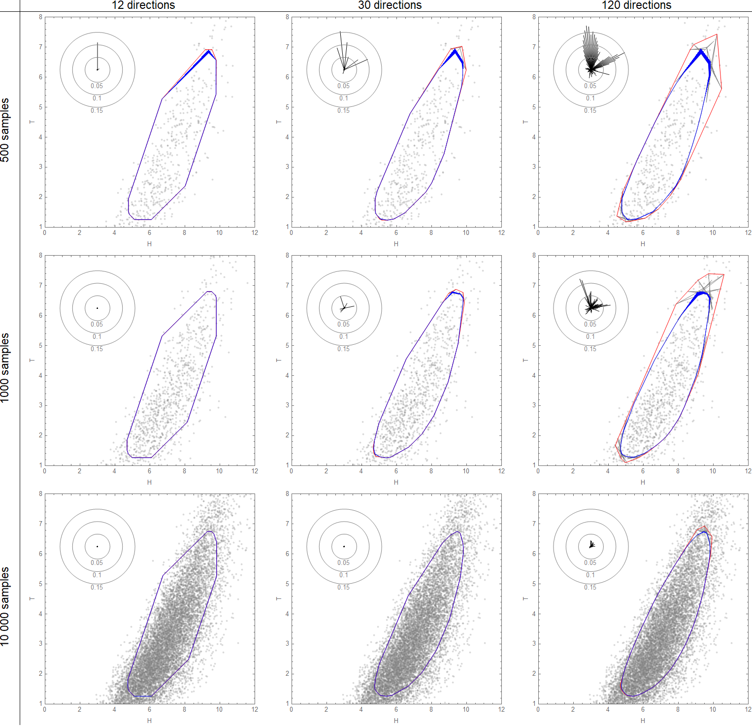
Figure 8 shows comparisons of results for different methods. The number of samples that the contours are based on is varied in the rows, but the samples are identical within each row. The number of unit vectors used to compute the contours is varied in the columns.
The direct sampling method of [36] is drawn in black. This method does not guarantee convex contours, but sometimes produce loops. Keeping the samples fixed, the loops tend to be larger as the number of unit vectors increase, which is undesirable. However, the loops tend to get smaller with increased number of samples. The convex hull of the black contours are drawn in red. Note that for the same number of samples, these red contours tend to get larger when the number of directions is increased, due to the larger loops.
Contours based on the Voronoi method are shown in blue. More precisely, blue regions are plotted, where the inner boundary correspond to the simple Voronoi method (i.e. Algorithm 6.1), and the outer boundary correspond to the corrected Voronoi method (i.e. Algorithm 6.2). Note that, unlike the other methods, the contours produced by the Voronoi methods do not diverge as the number of directions is increased. We also see that the shaded region is generally thin, indicating that the simple Voronoi method is a good approximation to the ’true’ environmental contour. The inset shows the error, i.e. the difference between the two Voronoi methods in the various directions. The directions with high error corresponds to directions where the direct method of [36] produces loops, i.e. the Voronoi method provides a warning for directions where more sampling may be needed.
7.2 3D example
To illustrate the Voronoi approach in three dimensions, we include an example from [48]. The environmental variables of interest are the significant wave height, , the zero-upcrossing wave period, , and the 10-minute mean wind speed at a particular height, . Their joint distribution is modelled using a conditional modelling approach [56, 57], and can be expressed as
| (17) |
is a 3-parameter Weibull distribution for significant wave height, with scale parameter , shape parameter , and location parameter .
is a conditional log-normal distribution for wave period, where the model parameters are a function of significant wave height as outlined in e.g. [1, 40], i.e.
| (18) | ||||
The parameters , are estimated from data.
is a conditional 2-parameter Weibull distribution with parameters modelled as functions of significant wave height as suggested by [1, 58, 59]. The scale parameter, , and shape parameter, , are modelled as
| (19) | ||||
For the significant wave height and wave period, parameters corresponding to average world wide operations of ships according to appendix C of [1] are assumed, as summarised in Table 2. For the conditional distribution of wind speed, the average sectoral parameters reported in [58, 59] will be assumed, as summarised in Table 2. It is noted that the parameter is omitted in [58], so this is simply set to 1 in this study.
Figure 9 shows the result of applying the Voronoi methods (simple and corrected) to the example described above. As can be seen, the simple method and corrected method are very similar, indicating that the simple Voronoi method is a good approximation for the ’true’ environmental contour.
| 3-p Weibull () | ||||
| average World wide trade | 1.798 | 1.214 | 0.856 | |
| Conditional log-normal () | i = 1 | i = 2 | i = 3 | |
| average World wide trade | ai | -1.010 | 2.847 | 0.075 |
| bi | 0.161 | 0.146 | -0.683 | |
| Conditional 2-p Weibull () | i = 1 | i = 2 | i = 3 | |
| average directional sector | ci | 2.58 | 0.12 | 1.60 |
| di | 4.6 | 2.05 | 1 | |

8 Concluding remarks
In this paper, a novel algorithm for constructing environmental contours has been presented, based on a geometric interpretation of environmental contours as Voronoi cells. One advantage of this approach is that many software libraries exist for Voronoi cell computation, making the algorithm simple to implement. Another advantage is that the Voronoi method also makes it easy to compute environmental contours in higher than two dimensions. The Voronoi environmental contours are not guaranteed to be proper, but with a simple modification to the algorithm, valid environmental contours can always be constructed from improper Voronoi environmental contours.
The Voronoi geometric interpretation also has given new intuition and theoretical insights about environmental contours, including representation and existence theorems for proper convex environmental contours. The presented analytical formula provides another alternative algorithm to compute environmental contours. Interestingly, this formula has an analogy in shadow systems and can be interpreted as an inverse Gauss map [60, 61, 62]. Further exploration of this correspondence between environmental contours and shadow functions could potentially reveal new insights in both domains, and potentially provide some information on the class of random variables for which proper environmental contours exist.
Acknowledgements
This work has been supported by grant 276282 from the Research Council of Norway (RCN) and DNV GL Group Technology and Research. Parts of the work has also been carried out within the research project ECSADES, with support from RCN under the MARTEC II ERA-NET initiative; project no. 249261/O80.
Appendix A Proof of Lemma 4.1
Proving the first statement is trivial, as by definition means that
for any .
So, in particular, we have that
.
To prove the second statement we use that
That is, a point in the interior of is also in the intersection of all interior half-spaces. Hence, for all . And so by the same argument as above we have that .
To prove the converse, we first observe that if , then
then there exists some where (by the supporting hyperplane theorem)
which means that , and if then we have already
shown that for some .
Putting this together we get that ,
and hence .
As for the final statement, we first recall that a point is in if and only if , or equivalently , for any . We first observe that
| (20) |
and so,
Hence, using the second statement of the Lemma, we have that if then , and so for any which completes the proof.
∎
Appendix B Proof of Proposition 4.2
First we recall that by definition .
Using Lemma 4.1 we then have
, and also
for .
Since the proof is completed by observing that
∎
Appendix C Proof of Proposition 4.3
The proof will follow from the Voronoi-Delaunay duality, which tell us that the Voronoi cells are convex polytopes with vertices corresponding to circumcenters of the Delaunay simplices. In particular, the vertices of are the circumcenters of the simplices in , where is any Delaunay triangulation of the point set .
Assume that is such a Delaunay triangulation, and that there exists a point such that and are not connected by . This means (by definition) that any simplex in containing does not contain , and vice versa. Hence,
We now let denote the unit vector corresponding to , i.e. . Making use of Lemma 4.1 we then observe that
| (21) |
This means that, either 1) , or 2) that there exists some vertex of such that . From Proposition 4.2 we have that . Since we assume that is a proper convex environmental contour, , and so
| (22) |
From (21) and (22) we can therefore conclude that there exists some vertex of such that .
We then observe that
| (23) |
This follows from the definition of and the set , which says that is the reflection of with respect to the hyperplane . Now, since is also a vertex of , then is the circumcenter of a Delaunay simplex , with . From (23) we see that also lies on this circum-hypersphere, together with . Hence, if the Delaunay triangulation was unique, we could conclude that , which contradicts the initial assumption that and are not connected in .
In the case where there is no unique Delaunay triangulation of the point set , the fact that and lie on the same circum-hypersphere of some Delaunay simplex lets us conclude that there exists some Delaunay triangulation where and are part of the same simplex. We can therefore conclude that, if there exists a Delaunay triangulation that does not connect and , then there must exist a different Delaunay triangulation that connects and .
∎
Appendix D Proof of Proposition 5.1
For any we first recall that the existence of some follows from the definition of proper convex environmental contours. We then note that, as any element of is of the form , we have that
| (24) |
Now if we have that (by definition), and hence , which means that .
The statement that means that there are no such that lies in the interior of the ball . Assume, on the contrary, that there exists some . Then by definition. From (24) we then have that . We have assumed that , and so by Lemma 4.1 . Hence,
But this means that , which is impossible when .
∎
Appendix E Proof of Lemma 5.2
We first observe that the condition 1) is just a different way of stating that a point is on the hyperplane (alternatively, compute the norms as in (24) and note that ). That is, for any , we have .
Hence, by condition 1). Then, by Proposition 5.1 there exists some where , and . This means that the -dimensional closed ball , centered at with radius is tangent to at the point . As both and are differentiable -dimensional manifolds, they share the same -dimensional tangent space at . We let denote a basis for this tangent space.
From the above argument, it is clear that also satisfies both of the criteria in the Lemma, as 1) and 2) is orthogonal to at since is orthogonal to at .
Hence, starting with a pair that satisfies the two conditions of the Lemma, we have identified a point such that satisfies the same conditions. Using that and satisfy these conditions simultaneously, we obtain
- 1.
,
- 2.
for any .
From these conditions we see that and for any . Hence, if is linearly independent of , we can conclude that .
Assume for some . Then . Then, by definition of the hyperplane , . But this means that , which is impossible.
We may therefore conclude that . By the same argument as above, if and are two elements of , then since and both satisfy the conditions of the Lemma, we must have . is therefore a singleton set, and we can conclude that .
∎
Appendix F Proof of Proposition 5.3
We first recall that if is a proper convex environmental contour, then for any there exists some such that , and so .
Then, if is a mapping such that the assumptions and conditions of Lemma 5.2 hold for any pair , Lemma 5.2 lets us conclude that for any .
Hence, .
∎
Appendix G Proof of Theorem 5.4
If the the -level percentile function is continuously differentiable on the unit -sphere, then as , the set is a differentiable manifold. Hence, the assumptions of Lemma 5.2 are satisfied.
We first note that, as a consequence of Lemma 5.2, any supporting hyperplane intersects at a single point, which means that is strictly convex. For details we refer to the proof of Lemma 5.2 in Appendix E, where we observe that is a singleton set for any , as the pair satisfies the conditions in Lemma 5.2 for any . (And for any we have for some as is proper).
We will show that the proposed parametrization in the theorem is valid using Lemma 5.2 and Proposition 5.3. That is, for any , we must show that
- 1.
, and
- 2.
is orthogonal to at ,
for . To simplify the notation we will suppress writing out the dependency on , and write
Using (9) we can express in terms of :
where we made use of the property that (i.e. the identity operator). Note that the metric tensor is invertible because we have assumed a regular parametrization (and so has full rank).
To show condition (1) above, we can just compute the norms
Here we have used the fact that .
To show condition (2) we will use that the columns of form a basis for the tangent space of at . The orthogonality condition (2) is therefore equivalent to saying that . But this follows from the definition of , as , and hence
Using Proposition 5.3 we may then conclude that, given an atlas on where each is a regular parametrization, the corresponding charts is an atlas on . Finally, differentiability of then follows from the given expression for as a function of .
∎
Appendix H Proof of Lemma 5.5
We first observe that, as a direct consequence of Definition 2.1, admits a proper convex environmental contour if and only if every hyperplane is a supporting hyperplane of . That is, if and only if for all .
Hence, if admits a proper convex environmental contour, we can select which (by Lemma 4.1) satisfies the condition.
If does not admit a proper convex environmental contour, then there is some hyperplane that does not intersect . Hence, for any we have , and by Lemma 4.1 there must exist some where .
∎
Appendix I Proof of Lemma 5.6
Dropping the dependency on and for simpler notation, we may write
as and . This means that . Similarly, we observe that
as by definition. From the chain rule we then get . Since the hyperplane has normal vector , we can conclude that is tangential to at .
∎
Appendix J Proof of Theorem 5.7
To simplify notation, we drop the dependency and the index of the parametrization.
Assume is true and let denote the closed convex set. Then Lemma 5.6 implies that all hyperplanes are supporting hyperplanes of , and so is a proper convex environmental contour. The fact that comes as a direct consequence of Theorem 5.4, so we have that .
To show that , we first note that when admits a proper convex environmental contour, then since (see Lemma 5.6) it follows from Lemma 4.1 that for all and . For the converse, assume that does not admit a proper convex environmental contour. Then from Lemma 5.5 there exists some such that for any we can find some where . In forms of the given parametrization, this means that we can find some and where for any . As we have that . Hence .
Finally, follows from the fact that which means that .
∎
Appendix K Proof of Corollary 5.8
From statement in Theorem 5.7, attains a local minimum at , which means that the matrix is positive semi-definite . Suppressing the notation and we can write
| (25) |
The second term in the last line of (25) above can be rewritten in terms of the metric tensor :
because and .
The third term in the last line of (25) can be expressed as . In index form (using Einstein summation convention) we may write the matrix elements of this term as , where we have recognised the Christoffel symbols of the first and second kind, i.e. and . Therefore we may write
| (26) |
The term in brackets correspond to the Hessian on a Riemann manifold, and we may therefor write
| (27) |
∎
References
- [1] D. GL, Environmental Conditions and Environmental Loads, DNV GL, september 2019 Edition, DNVGL-RP-C205 (2019).
- [2] NORSOK, NORSOK Standard N-003:2017. Action and action effects, edition 3 (2017).
- [3] S. Haver, Analysis of uncertainties related to the stochastic modelling of ocean waves, Tech. Rep. UR-80-09, Norges tekniske høgskole (1980).
- [4] S. Haver, On the joint distribution of heights and periods of sea waves, Ocean Engineering 14 (1987) 359–376.
- [5] S. Winterstein, T. Ude, C. Cornell, P. Bjerager, S. Haver, Environmental parameters for extreme response: Inverse FORM with omission factors, in: Proc. 6th International Conference on Structural Safety and Reliability, 1993.
- [6] S. Haver, S. Winterstein, Environmental contour lines: A method for estimating long term extremes by a short term analysis, Transactions of the Society of Naval Architects and Marine Engineers 116 (2009) 116–127.
- [7] B. J. Leira, A comparison of stochastic process models for definition of design contours, Structural Safety 30 (2008) 493–505.
- [8] J. M. Niedzwwecki, J. van de Lindt, J. Yao, Estimating extreme tendon response using environmental contours, Engineering Structures 20 (1998) 601–607.
- [9] S. R. Winterstein, A. K. Jha, S. Kumar, Reliability of floating structures: Extreme response and load factor design, Journal of Waterway, Port, Coastal and Ocean Engineering 125 (1999) 163–169.
- [10] G. S. Baarholm, T. Moan, Application of contour line method to estimate extreme ship hull loads considering operational restrictions, Journal of Ship Research 45 (2001) 228–240.
- [11] K. Saranyasoontorn, L. Manuel, Design loads for wind turbines using the environmental contour method, in: 44th AIAA Aerospace Sciences Meeting and Exhibit, American Institute of Aeronautics and Astronautics (AIAA), 2006, pp. AIAA 2006–1365.
- [12] G. S. Baarholm, H. Sverre, C. M. Larsen, Wave sector dependent contour lines, in: Proc. 26th International Conference on Offshore Mechanics and Arctic Engineering (OMAE 2007), American Society of Mechanical Engineers (ASME), 2007.
- [13] G. S. Baarholm, S. Haver, Application of environmental contour lines - a summary of a number of case studies, in: Proc. International Conference on Floating Structures for Deepwater Operations, ASRANet, 2009.
- [14] G. S. Baarholm, S. Haver, O. D. Økland, Combining contours of significant wave height and peak period with platform response distributions for predicting design response, Marine Structures 23 (2010) 147–163.
- [15] P. Jonathan, K. Ewans, J. Flynn, On the estimation of ocean engineering design contours, in: Proc. 30th International Conference on Ocean, Offshore and Arctic Engineering (OMAE 2011), American Society of Mechanical Engineers (ASME), 2011.
- [16] S. Haver, K. Bruserud, Environmental contour method: An approximate method for obtaining characteristic response extremes for design purposes, in: Proc. 13th International Workshop on Wave Hindcasting and Forecasting & 4th Coastal Hazard Symposium, 2013.
- [17] M. J. Muliawan, Z. Gao, T. Moan, Application of the contour line method for estimating extreme responses in the mooring lines of a two-body floating wave energy converter, Journal of Offshore Mechanics and Arctic Engineering 135 (2013) 031301:1–10.
- [18] C. Armstrong, C. Chin, I. Penesis, Y. Drobyshevski, Sensitivity of vessel response to environmental contours of extreme sea states, in: Proc. 34th International Conference on Ocean, Offshore and Arctic Engineering (OMAE 2015), American Society of Mechanical Engineers (ASME), 2015.
- [19] L. D. Lutes, S. R. Winterstein, A dynamic inverse FORM method: Design contours for load combination problems, Probabilistic Engineering Mechanics 44 (2016) 118–127.
- [20] Q. Li, Z. Gao, T. Moan, Modified environmental contour method for predicting long-term extreme responses of bottom-fixed offshore wind turbines, Marine Structures 48 (2016) 15–32.
- [21] A. C. Eckert-Gallup, C. J. Sallaberry, A. R. Dallman, V. S. Neary, Application of principal component analysis (PCA) and imrpoved joint probability distributions to the inverse first-order reliability method (I-FORM) for predicting extreme sea states, Ocean Engineering 112 (2016) 307–319.
- [22] E. Vanem, A simple approach to account for seasonality in the description of extreme ocean environments, Marine Systems & Ocean Technology 13 (2018) 63–73.
- [23] A. B. Huseby, E. Vanem, M. H. Barbosa, Environmental contours for mixtures of distributions, in: Proc. ESREL 2019, European Safety and Reliability Association(ESRA), 2019.
- [24] Z. S. Haghayeghi, M. J. Ketabdari, Development of environmental contours for circular and linear metocean variables, International Journal of Renewable Energy Research 7 (2017) 682–693.
- [25] F. Silva-González, E. Heredia-Zavoni, R. Montes-Iturrizaga, Development of environmental contours using Nataf distribution model, Ocean Engineering 58 (2013) 27–34.
- [26] R. Montes-Iturrizaga, E. Heredia-Zavoni, Environmental contours using copulas, Applied Ocean Research 52 (2015) 125–139.
- [27] Q. Derbanne, G. da Hauteclocque, A new approach for environmental contour and multivariate de-clustering, in: Proc. 38th International Conference on Ocean, Offshore and Arctic Engineering (OMAE 2019), American Society of Mechanical Engineers (ASME), 2019.
- [28] K. R. Dahl, A. B. Huseby, Buffered environmental contours, in: Proc. ESREL 2018, European Safety and Reliability Association(ESRA), 2018.
- [29] W. Chai, B. J. Leira, Environmental contours based on inverse SORM, Marine Structures 60 (2018) 34–51.
- [30] A. F. Haselsteiner, J.-H. Ohlendorf, W. Wosniok, K.-D. Thoben, Deriving environmental contours from highest density regions, Coastal Engineering 123 (2017) 42–51.
- [31] R. Montes-Iturrizaga, E. Heredia-Zavoni, Assessment of uncertainty in environmental contours due to parametric uncertainty in models of the dependence structure between metocean variables, Applied Ocean Research 64 (2017) 86–104.
- [32] E. Vanem, O. Gramstad, E. M. Bitner-Gregersen, A simulation study on the uncertainty of environmental contours due to sampling variability for different estimation methods, Applied Ocean Research 91 (2019) 101870.
- [33] E. Vanem, Environmental contours for describing extreme ocean wave conditions based on combined datasets, Stochastic Environmental Research and Risk Assessment 33 (2019) 957–971.
- [34] L. Manuel, P. T. Nguyen, J. Canning, R. G. Coe, A. C. Eckert-Gallup, N. Martin, Alternative approaches to develop environmental contours from metocean data, Journal of Ocean Engineering and Marine Energy 4 (2018) 293–310.
- [35] E. Ross, O. C. Astrup, E. Bitner-Gregersen, N. Bunn, G. Feld, B. Gouldby, A. Huseby, Y. Liu, D. Randell, E. Vanem, P. Jonathan, On environmental contours for marine and coastal design, Ocean Engineering 195 (2020) 106194.
- [36] A. B. Huseby, E. Vanem, B. Natvig, A new approach to environmental contours for ocean engineering applications based on direct Monte Carlo simulations, Ocean Engineering 60 (2013) 124–135.
- [37] A. B. Huseby, E. Vanem, B. Natvig, Alternative environmental contours for structural reliability analysis, Structural Safety 54 (2015) 32–45.
- [38] A. B. Huseby, E. Vanem, B. Natvig, A new Monte Carlo method for environmental contour estimation, in: Proc. ESREL 2014, European Safety and Reliability Association(ESRA), 2014.
- [39] A. B. Huseby, E. Vanem, K. Eskeland, Evaluating properties of environmental contours, in: Proc. ESREL 2017, European Safety and Reliability Association(ESRA), 2017.
- [40] E. Vanem, E. M. Bitner-Gregersen, Alternative environmental contours for marine structural design - a comparison study, Journal of Offshore Mechanics and Arctic Engineering 137 (2015) 051601:1–8.
- [41] E. Vanem, A comparison study on the estimation of extreme structural response from different environmental contour methods, Marine Structures 56 (2017) 137–162.
- [42] E. Vanem, B. Guo, E. Ross, P. Jonathan, Comparing different contour methods with response-based methods for extreme ship response analysis, Marine Structures 69 (2919) 102680.
- [43] R. Nerzic, C. Frelin, M. Prevesto, V. Quiniou-Ramus, Joint distribution of wind/waves/current in West Africa and derivation of multivariate extreme I-FORM contours, in: Proc. 17th International Offshore and Polar Engineering Conference (ISOPE 2007), The International Society of Offshore and Polar Engineering (ISOPE), 2007.
- [44] J. van de Lindt, J. Niedzwecki, Environmental contour analysis in earthquake engineering, Engineering Structures 22 (2000) 1661–1676.
- [45] K. Saranyasoontorn, L. Manuel, Efficient models for wind turbine extreme loads using inverse reliability, Journal of Wind Engineering and Industrial Aerodynamics 92 (2004) 789–804.
- [46] P. Orsero, E. Fontaine, V. Quiniou, Reliability and response based design of a moored FPSO in West Africa using multivariate environmental contours and response surfaces, in: Proc. 17th International Offshore and Polar Engineering Conference (ISOPE 2007), The International Society of Offshore and Polar Engineering (ISOPE), 2007.
- [47] R. Montes-Iturrizaga, E. Heredia-Zavoni, Multivariate environmental contours using C-vine copulas, Ocean Engineering 118 (2016) 68–82.
- [48] E. Vanem, 3-dimensional environmental contours based on a direct sampling method for structural reliability analysis of ships and offshore structures, Ships and Offshore Structures 14 (2018) 74–85.
- [49] N. Raillard, M. Prevesto, H. Pineau, 3-d environmental extreme value models for the tension in a mooring line of a semi-submersible, Ocean Engineering 184 (2019) 23–31.
- [50] I. Leonard, J. Lewis, Geometry of Convex Sets, Wiley, 2015.
- [51] A. Okabe, B. Boots, K. Sugihara, S. N. Chiu, Spatial Tessellations: Concepts and Applications of Voronoi Diagrams, 2nd Edition, Series in Probability and Statistics, John Wiley and Sons, Inc., 2000.
- [52] F. M. Schaller, S. Kapfer, M. Evans, M. J.F. Hoffmann, T. Aste, M. Saadatfar, K. Mecke, G. W. Delaney, G. Schröder-Turk, Set Voronoi diagrams of 3D assemblies of aspherical particles, Philosophical Magazine 93.
- [53] F. Aurenhammer, Voronoi diagrams - a survey of a fundamental geometric data structure, ACM Comput. Surv. 23 (3) (1991) 345–405.
- [54]
A. B. Huseby, K. R. Dahl,
Lecture
notes STK4400 - Risk and reliability analysis (09 2018).
URL https://www.uio.no/studier/emner/matnat/math/STK4400/h18/notater/week-41.pdf - [55] G. Marsaglia, Choosing a point from the surface of a sphere, Ann. Math. Statist. 43 (2) (1972) 645–646.
- [56] E. Bitner-Gregersen, Joint long term models of met-ocean parameters, in: C. Guedes Soares (Ed.), Marine Technology and Engineering: CENTEC Anniversary Book, CRC Press, 2012.
- [57] E. M. Bitner-Gregersen, Joint met-ocean description for design and operation of marine structures, Applied Ocean Research 51 (2015) 279–292.
- [58] E. Bitner-Gregersen, S. Haver, Joint environmental model for reliability calculations, in: Proc. 1st International Offshore and Polar Engineering conference (ISOPE 1991), The International Society of Offshore and Polar Engineering (ISOPE), 1991.
- [59] E. Bitner-Gregersen, S. Haver, Joint long term description of environmental parameters for structural response calculation, in: Proc. 2nd International Workshop on Wave Hindcasting and Forecasting, 1989.
- [60] G. C. Shephard, Shadow systems of convex sets, Israel Journal of Mathematics 2 (4) (1964) 229–236.
- [61]
C. l. Epstein, Convex
regions, shadows, and the Gauss map.
URL https://www.math.upenn.edu/˜cle/papers/slatgm.pdf - [62] H. Martini, L. Montejano, D. Oliveros, Bodies of constant width, Springer, 2019.