Goodness-of-fit tests for parametric regression models with circular responseThanks: Research group MODES, CITIC, Department of Mathematics, Faculty of Computer Science, Universidade da Coruña, Campus de Elviña s/n, 15071, A Coruña, SpainThanks: Department of Statistics, Mathematical Analysis and Optimization, Faculty of Mathematics, Universidade de Santiago de Compostela, Rúa Lope Gómez de Marzoa s/n, 15782, Santiago de Compostela, Spain
Abstract
Testing procedures for assessing a parametric regression model with circular response and -valued covariate are proposed and analyzed in this work both for independent and for spatially correlated data. The test statistics are based on a circular distance comparing a (non-smoothed or smoothed) parametric circular estimator and a nonparametric one. Properly designed bootstrap procedures for calibrating the tests in practice are also presented. Finite sample performance of the tests in different scenarios with independent and spatially correlated samples, is analyzed by simulations.
Keywords: Model checking, Circular data, Local polynomial regression, Spatial correlation, Bootstrap
Introduction
In many scientific fields, such as oceanography, meteorology or biology, data are angular measurements (points in the unit circle of a circular variable), which are accompanied by auxiliary observations of other Euclidean random variables. The joint behavior of these circular and Euclidean variables can be analyzed by considering a regression model, allowing at the same time to explain the possible relation between the variables and also to make predictions on the variable of interest. Parametric regression estimators for linear-circular models (circular response and Euclidean covariates) with independent data have been studied by Fisher and Lee 1992, Presnell et al. 1998, and Kim and SenGupta 2017, among others. In the presence of spatial correlation, Jona-Lasinio et al. 2012, Wang and Gelfand 2014, Lagona et al. 2015 and Mastrantonio et al. 2016 for instance, employed parametric methods to model circular spatial processes. Alternatively, nonparametric regression approaches can be used to deal with these inference problems. For this purpose, kernel-type estimators of the regression function in a model with a circular response and a -valued covariate have been introduced by Meilán-Vila et al. 2020a; Meilán-Vila et al. 2020c. Notice that if the bandwidth matrix is appropriately chosen, these methods provide more flexible estimators than those obtained using parametric approaches, avoiding misspecification problems. However, if a parametric regression model is assumed and it holds, parametric methods usually provide estimators which are more efficient and easier to interpret. In this context, goodness-of-fit tests can be designed, providing a tool for assessing a general class of parametric linear-circular regression models.
There is a substantial literature on testing parametric regression models involving Euclidean data, including Kozek 1991, Härdle and Mammen 1993, González Manteiga and Vilar Fernández 1995, Biedermann and Dette 2000, Park et al. 2015, Meilán-Vila et al. 2020b, and Meilán-Vila et al. 2020d, among others. See González-Manteiga and Crujeiras 2013 for a review. The previous testing procedures are based on measuring differences between a suitable parametric estimator under the null hypothesis and a nonparametric one. Specifically, -norm or supremum-norm tests, among others, can be employed for regression models with Euclidean responses and covariates. In the context of regression models with directional response and directional or Euclidean explanatory variables, the literature on goodness-of-fit tests is relatively scarce. In this setting, Deschepper et al. 2008 proposed an exploratory tool and a lack-of-fit test for circular-linear regression models (Euclidean response and circular covariates). The same problem was studied by García-Portugués et al. 2016, using nonparametric methods. The authors proposed a testing procedure based on the weighted squared distance between a smooth and a parametric regression estimator, where the smooth regression estimator was obtained by a projected local regression on the sphere. However, the problem of assessing a certain class of parametric linear-circular regression models, that is, for a regression model with circular response and -valued covariates (up to the authors knowledge) has not been considered in the statistical literature yet, neither for independent nor for spatially dependent observations.
In this work, new approaches for testing a linear-circular parametric regression model (circular response and -valued covariate) are proposed and analyzed both for independent and spatially correlated errors. The test statistics employed in these procedures are based on a comparison between a (non-smoothed or smoothed) parametric fit under the null hypothesis and a nonparametric estimator of the circular regression function. More specifically, two different test statistics are considered. In the first one, the parametric estimator of the regression function under the null hypothesis is directly used, while in the second one, a smooth version of this estimator is employed. Notice that, in this framework, a suitable measure of circular distance must be employed (see Jammalamadaka and SenGupta 2001, Section 1.3.2). The null hypothesis that the regression function belongs to a certain parametric family if the distance between both fits exceeds a certain threshold. To perform the parametric estimation, a circular analog to least squares regression is used (Fisher and Lee 1992; Lund 1999, see). For the nonparametric alternative, kernel-type regression estimators (Meilán-Vila et al. 2020a; Meilán-Vila et al. 2020c) are considered.
For the application in practice of the proposals, the test statistics should be accompanied by a calibration procedure. In this case, this is not based on the asymptotic distribution, given that the convergence to the limit distribution under the null hypothesis will presumably be too slow. Different bootstrap methods are designed and their performance is analyzed and compared in empirical experiments. For independent data, standard resampling procedures adapted to the context of regression models with circular response are used: a parametric circular residual bootstrap (PCB) and a nonparametric circular residual bootstrap (NPCB). The PCB approach consists in using the residuals obtained from the parametric fit in the bootstrap algorithm. If the circular regression function belongs to the parametric family considered in the null hypothesis, then the residuals will tend to be quite similar to the theoretical errors and, therefore, it is expected that the PCB method has a good performance. Following the proposal by González-Manteiga and Cao 1993, the NPCB method aims to increase the power of the test and, for this purpose, the residuals obtained from the nonparametric fit are the ones employed in the bootstrap procedure. The previous resampling procedures (PCB and NPCB) for independent data must be properly adapted for handling spatial correlation. Two specific procedures for test calibration which take the spatial correlation into account are also introduced: a parametric spatial circular residual bootstrap (PSCB) and a nonparametric spatial circular residual bootstrap (NPSCB). Similarly to the PCB, but now for spatially correlated errors, the PSCB considers the residuals obtained from the parametric fit under the null hypothesis. The relevant difference between PCB and PSCB is that, in order to mimic the dependence structure of the errors, a spatial circular process is fitted to the residuals in PSCB. Samples coming from the fitted process are employed in the bootstrap algorithm. The steps followed in NPSCB are similar at those employed in PSCB, but the residuals are obtained from the nonparametric regression estimator.
This paper is organized as follows. Section 2 is devoted to present some ideas of goodness-of-fit tests for circular regression models. The parametric and nonparametric circular regression estimators employed in the test statistics are presented in Sections 2.1 and 2.2, respectively. Section 2.3 introduces the testing problem and the proposed test statistics. A description of the calibration algorithms considered is given in Section 2.4. Section 2.5 contains a simulation study for assessing the performance of the tests when using the PCB and NPCB resampling approaches to approximate the sampling distribution of the test statistics. The extension of the testing procedures for spatially correlated data is presented in Section 3. Section 3.1 contains bootstrap approaches to calibrate the tests in this spatial framework. A simulation study for assessing the performance of the tests using PSCB and NPSCB methods is provided in Section 3.2. Finally, some conclusions and ideas for further research are provided in Section 4.
Goodness-of-fit tests for circular regression models with independent data
Let be a random sample from , where is a circular random variable taking values on , and is a random variable with density and support on . Assume that the following regression model holds:
| (1) |
where is a circular regression function, and , is an independent sample of a circular variable , with zero mean direction and finite concentration. This implies that . Additionally, the following notation is used: , , and .
Considering the regression model (1), one of the aims of the present research is to propose and study different testing procedures to assess the suitability of a general class of parametric circular regression models. Specifically, in this work, we focus on the following testing problem:
| (2) |
where is a link function mapping the real line onto the circle. As pointed out in Section 1, the procedure proposed in this work consists in comparing a (non-smoothed or smoothed) parametric fit with a nonparametric estimator of the circular regression function , measuring the circular distance between both fits and employing this distance as a test statistic. The parametric and nonparametric estimation methods considered in this proposal are described in what follows.
Parametric circular regression estimator
As mentioned in the Introduction, our proposal requires a parametric estimator of the circular regression function , once a parametric family is set as the null hypothesis. Notice that, for instance, the procedures based on least squares for Euclidean data, are not appropriate when the response variable is of circular nature. Minimizing the sum of squared differences between the observed and predicted values may lead to erroneous results, since the squared difference is not an appropriate measure on the circle.
A circular analog to least squares regression for models with a circular response and a set of Euclidean covariates was presented by Lund 1999. Specifically, assume the regression model (1) holds and consider , where is a certain parametric circular regression model with parameter vector . A parameter estimate of could be obtained by minimizing the sum of the circular distances between the observed and predicted values as follows:
| (3) |
The value of the parameter minimizing the previous expression will be used to construct the parametric circular regression estimator, namely, .
An equivalent parameter estimator can be obtained using a maximum-likelihood approach (Lund 1999). If it is assumed that the response variable (conditional on ) has a von Mises distribution with mean direction given by and concentration parameter , the maximum likelihood estimator of maximizes the following expression
| (4) |
Notice that the circular least squares estimator given in (3) also maximizes the expression (4) and, therefore, as pointed out before, assuming a von Mises distribution, the circular least squares estimator coincides with the maximum likelihood estimator. For further details see Lund 1999.
Assuming that the response variable follows a von Mises distribution and considering as the parametric family given in (2), an iteratively reweighted least squares algorithm can be used to compute the maximum likelihood estimators of , and (Lund 1999; Fisher and Lee 1992, see). The extension of these results to the case of a generic parametric family has not been explicetly considered.
Nonparametric circular regression estimator
A nonparametric regression estimator for in model (1) is presented in this section. Notice that the circular regression function is the conditional mean direction of given which, at a point , can be defined as the minimizer of the risk . Specifically, the minimizer of this cosine risk is given by , where and . Therefore, replacing and by appropriate estimators, an estimator for can be directly obtained. In particular, a whole class of kernel-type estimators for at can be defined by considering local polynomial estimators for and . Specifically, estimators of the form:
| (5) |
are considered, where for any integer , and denote the th order local polynomial estimators (with bandwidth matrix ) of and , respectively. The special cases and yield a Nadaraya–Watson (or local constant) type estimator and a local linear type estimator of , respectively. Asymptotic properties of these estimators, considering model (1), have been studied by Meilán-Vila et al. 2020c.
The test statistics
In this section, in order to check if the circular regression function belongs to a general class of parametric models, goodness-of-fit tests are presented. We consider the testing problem (2).
Test statistics to address (2) are proposed and studied. The first approach considers a weighted circular distance between the nonparametric and parametric fits:
| (6) |
for , where is a weight function that helps in mitigating possible boundary effects. The estimators , for , are the Nadaraya-Watson or the local linear type estimators of the circular regression function , given in (5). The parametric estimator was described in Section 2.1.
The second approach is similar to the first one, but considering a smooth version of the parametric fit:
| (7) |
where , for , are smooth versions of the parametric estimator , which are given by:
with
being and .
In order to formally address problem (2) using the test statistics and given in (6) and in (7), respectively, it is essential to approximate the distribution of the test statistic under the null hypothesis. Deriving the asymptotic distribution of the statistics is out of the scope of this work. However, some guidelines to compute these expressions are provided in Section 4. For the application in practice of our proposal, the distribution of the tests under the null hypothesis is approximated using bootstrap procedures and analyzed through an empirical study.
If the null hypothesis in the testing problem given in (2) holds, then the (non-smoothed or smoothed) parametric fit and the nonparametric circular regression estimator will be similar and, therefore, the value of the test statistics and will be relatively small. Conversely, if the null hypothesis does not hold, the fits will be different and the value of and will be fairly large. So, the null hypothesis will be rejected if the circular distance between both fits exceeds a critical value. For a visual illustration of the performance of the tests (where, for the sake of simplicity, a model with a single covariate is considered), suppose that a sample of size is generated following model (1), with regression function (10), with , and random errors drawn from a von Mises distribution . If we want to test if using the test statistics given in (6) and in (7), the estimators , and (denoting by the smoothing parameter when ) must be computed. In this case, the estimator obtained from (3) is considered for the parametric fit. The local linear type estimator given in (5) is employed to compute the nonparametric counterpart. A triweight kernel and the optimal bandwidth obtained by minimizing the circular average squared error (CASE), defined as:
| (8) |
for and , are considered to compute and . Figure 1 shows in red lines the local linear type regression estimator (left panel), the parametric fit (center panel) and the smooth version of the parametric fit (right panel), with sample points and the circular regression function (black lines). It seems that all estimates are very similar and, therefore, the value of the test statistics and should be small, and consequently, there would possibly be no evidences against the assumption that the circular regression function belonging to the parametric family .
Notice that the test statistics given in (6) and in (7), respectively, depend on the bandwidth matrix (or on the bandwidth parameter , if ). A non-trivial problem in goodness-of-fit testing is the bandwidth choice, since the optimal bandwidth for estimation may not be the optimal one for testing (being not even clear what optimal means). For instance, Fan et al. 2001, Eubank et al. 2005 and Hart 2013 gave some strategies on bandwidth selection in testing problems. This issue was also discussed further in detail by Sperlich 2013. As usual in the context of goodness-of-fit tests for regression based on nonparametric smoothers, the performance of the test statistics will be analyzed for a range of bandwidths, in order to evaluate the impact of this parameter in the numerical results.
Calibration in practice
Once a suitable test statistic is available, in order to solve the testing problem (2), a procedure for calibration of critical values is required. This task can be done by means of bootstrap resampling algorithms.
In what follows, a description of two different bootstrap proposals designed to approximate the distribution (under the null hypothesis) of the tests statistics given in (6) and in (7) for independent data (PCB and NPCB) are presented. The main difference between them is the mechanism employed to obtain the residuals. As noted in the Introduction, the residuals in PCB come from the parametric regression estimator. On the other hand, for the NPCB algorithm, the residuals are obtained from the nonparametric regression estimator. In order to present the PCB and NPCB resampling methods, a generic bootstrap algorithm is described. No matter the method used, denotes the parametric or the nonparametric circular regression estimator.
In Step 1 of the previous algorithm, in the PCB approach, the circular regression function is estimated parametrically, employing the procedure described in Section 2.1. Alternatively, the NPCB tries to avoid possible misspecification problems by using more flexible regression estimation methods than those employed in PCB. Then, using the same arguments as in González-Manteiga and Cao 1993 to increase the power of the test, in the NPCB method, the nonparametric circular regression estimator given in (5) is employed in Step 1 of the bootstrap Algorithm 1.
Notice that the empirical distribution of the bootstrap test statistics can be employed to approximate the finite sample distribution of the test statistics and , under the null hypothesis. Denoting by (for ) the sample of the bootstrap test statistics given in (6) and in (7), and defining its quantile , the null hypothesis in (2) will be rejected if . Additionally, the -values of the test statistics () can be approximated by:
| (9) |
Simulation study
The finite sample performance of the proposed tests, using the bootstrap approaches described in Algortihm 1 for their calibration, is illustrated in this section with a simulation study, considering a regression model with a single real-valued covariate and also with a bidimensional one.
2.5.1 Simulation experiment with a single covariate
In order to study the performance of the proposed tests considering a regression model with a circular response and a single real-valued covariate, the parametric regression family is chosen. For different values of the regression function
| (10) |
is considered. Therefore, the parameter controls whether the null () or the alternative () hypotheses hold in problem (2). Values , , and are considered in the study. For each value of , 500 samples of sizes and are generated on the unit interval, following model (1) with regression function (10) and circular errors drawn independently from a von Mises distribution , for different values of (5, 10 and 15).
To analyze the behavior of the test statistics given in (6) and in (7) in the different scenarios, the bootstrap procedures described in Section 2.4 are applied, using replications. The non-smoothed or smoothed parametric fits used for constructing (6) and (7) are computed using the procedures given in Sections 2.1 and 2.3, respectively. The nonparametric fit is obtained using the estimator given in (5), for with a triweight kernel. We address the bandwidth selection problem by using the same procedure as the one used in Härdle and Mammen 1993, Alcalá et al. 1999, or Opsomer and Francisco-Fernández 2010, among others, applying the tests on a grid of several bandwidths. In order to use a reasonable grid of bandwidths, the optimal bandwidth selected by minimizing the CASE given in (8), for , is calculated for each scenario. In this case, the values of the CASE optimal bandwidths are in the interval . Therefore, the values of the bandwidth parameter are considered to compute both test statistics (6) and (7). The weight function used in both tests is , to avoid possible boundary effects.
Effect of sample size. Proportions of rejections of the null hypothesis, for a significance level , considering , and different sample sizes, are shown in Tables 1 and 2, when using and , respectively. If (null hypothesis) and using the Nadaraya–Watson type estimator, the proportions of rejections are certainly much lower than the expected values. Using this estimator, the test works fairly well when PCB is employed. NPCB provides really bad results. When the local linear type estimator is used, the proportions of rejections are similar to the theoretical level, although these proportions are quite affected by the value of . For alternative assumptions ( and ), as expected, as the sample size increases the proportions of rejections are larger and increase with . As pointed out before, substantial differences have been found when the local linear type estimator is employed, providing more satisfactory results than those obtained when the Nadaraya–Watson fit is used. Using the local linear estimator, NPCB presents a slightly better performance than PCB. Although both test statistics provide a similar behavior of the testing procedure, seems to give slightly better results.
Effect of . The performance of the tests (for ) is studied for and for different values of the concentration parameter in Tables 3 and 4, when using and , respectively. If and considering the local linear type estimator, the proportions of rejections are similar to the theoretical level when using both bootstrap approaches (PCB and NPCB). Results obtained when the Nadaraya–Watson fit is used are quite poor, specially when NPCB is employed. For alternative assumptions, as expected, large values of the concentration parameter lead to an increase in power, which justifies the correct performance of the bootstrap procedures. Considerable differences have been found if the Nadaraya–Watson or local linear type estimators are employed in the test statistics, especially when NPCB is used.
2.5.2 Simulation experiment with several covariates
The extension for regression models with a circular response and two covariates is analyzed in this section. For this purpose, the parametric regression family is chosen, and for different values of the regression function
| (11) |
being , is considered. For each value of (, , and ), 500 samples of sizes and are generated on a bidimensional regular grid in the unit square, following model (1), with regression function (11) and circular errors drawn from a von Mises distribution , for and . The bootstrap procedures described in Section 2.4 are applied, using replications. The non-smoothed or smoothed parametric fits used for constructing (6) and (7) are computed using the procedures given in Sections 2.1 and 2.3, respectively. The nonparametric fit is obtained using the estimator given in (5), for with a multiplicative triweight kernel. In order to simplify the calculations, the bandwidth matrix is restricted to a class of diagonal matrices with both equal elements. In this case, the diagonal elements of the CASE optimal bandwidths are in the interval . Therefore, diagonal bandwidth matrices with different values of , are considered to compute both test statistics (6) and (7). The weight function used in both tests is , to avoid possible boundary effects.
Effect of sample size. Proportions of rejections of the null hypothesis, for a significance level , considering , and different sample sizes, are shown Tables 5, when using . It can be observed that using both bootstrap methods (PCB and NPCB), the test has a reasonable behavior. If (null hypothesis) and considering the local linear estimator, the proportions of rejections are similar to the theoretical level. As for a single covariate, results using the Nadaraya–Watson type estimator and NPCB are really bad. For alternative assumptions ( and ), NPCB presents a slightly better performance than the PCB, when using the local linear type estimator. Notice that, in most of the cases, an increasing power of the test when the values of increase is observed. For all the scenarios, the power of the test becomes larger as the value of increases. Again, considerable differences have been found when the local linear type estimator is employed. Similar conclusions to those given for were obtained when the test statistic was employed (see Table 6).
Effect of . The performance of the bootstrap procedures is analyzed for and for different values of the concentration parameter when using , for , in Table 7. If , the proportions of rejections are similar to the theoretical level when using both bootstrap approaches (PCB and NPCB). For larger values of the concentration parameter , the bandwidth values providing an effective calibration must be smaller. For alternative assumptions, if the value of the concentration parameter is larger, an increasing power is obtained. In almost all scenarios, some differences have been found if the Nadaraya–Watson or the local linear type estimators are employed in the test statistics. Results considering the test statistic are summarized in Table 8. Similar conclusions to those provided for were obtained.
Goodness-of-fit tests for circular regression models with spatially correlated data
The testing problem (2) is addressed in Section 2 for independent data, by constructing weighted circular test statistics. In this section, these test statistics are also analyzed considering a linear-circular regression model with spatially correlated errors.
Assume the linear-circular regression model given in (1), but supposing that the circular errors are spatially correlated. More specifically, we consider the linear-circular regression model given in (1):
| (12) |
where is a smooth trend or regression function and the are random angles, such that, , and additionally, satisfying in this dependence framework that
with for , and . The continuous stationary correlation functions satisfy , , and , for any , and . The subscript in indicates that the correlation functions vary with (specifically, the correlation functions are assumed to be short-range and shrink as goes to infinity). Note also that the subscript does not correspond to an integer sequence and it just indicates if the correlation corresponds to the sine process (), the cosine process () or if it is the cross-correlation between them ().
In order to solve the testing problem (2) in this context, the estimator described in Section 2.1 is likewise employed for the parametric fit. Probably, more accurate results would be obtained if an estimator taking the spatial dependence structure into account is considered. However, the problem of estimating parametrically the regression function accounting for the dependence structure (up to our knowledge) has not been considered in the statistical literature. Some guidelines about a possible iterative least squares estimator (taking the possible spatial dependence structure into account) are provided in Section 4. Kernel-type estimators given in (5) are employed for the nonparametric fit. These nonparametric estimators have been studied in Meilán-Vila et al. 2020a in the context of spatially correlated data.
For illustration purposes, a sample of size is generated on a bidimensional regular grid in the unit square, assuming the linear-circular regression model (12), with regression function (11), being . The circular spatially correlated errors , , are drawn from a wrapped Gaussian spatial process (Jona-Lasinio et al. 2012) with the following steps:
where is a realization of a real-valued Gaussian spatial process, where each observation can be decomposed as:
| (13) |
being the mean and random variables of a zero mean Gaussian spatial process with . The variance of is denoted by and is a continuous stationary correlation function satisfying , , and , . Note that a realization of this wrapped Gaussian spatial process can be written in vector form as , with mean direction vector , being a vector with every entry equal to 1, and covariance matrix , where is the -entry of the correlation matrix .
In this particular example, the circular spatially correlated errors are drawn from a wrapped Gaussian spatial process, considering that, in (13), and is a zero mean process with exponential covariance structure:
| (14) |
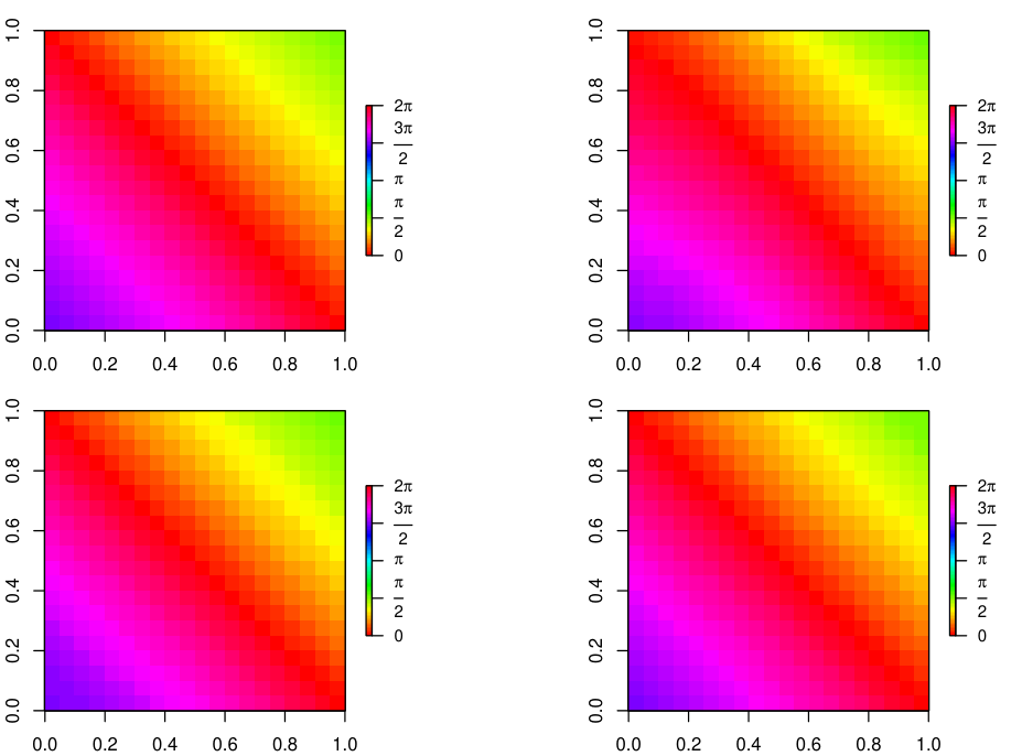
with and . In order to test if being , using the test statistics given in (6) and in (7), , and fits must be computed. For the parametric counterpart, the estimator obtained from (3) is employed, while local linear type estimators are used for the nonparametric smoothers. A multiplicative triweight kernel and the optimal bandwidth obtained by minimizing the CASE, given in (8), of the local linear type estimator are considered to compute and . Figure 2 shows the theoretical circular regression function (11), with (top left panel), the local linear type regression estimator (top right panel), the parametric fit (bottom left panel) and the smooth version of the parametric fit (bottom right panel). It can be seen that estimates at top right, bottom left and bottom right panels seem to be very similar and, therefore, the value of the test statistics and should be small. Consequently, the formal application of the tests will probably lead to assert that there is no evidences against the assumption that the regression function belongs to the parametric family , with .
Practical methods to calibrate the test statistics and given in (6) and in (7) for spatially correlated data are presented in the following section.
Calibration in practice
This section is devoted to present bootstrap resampling methods to calibrate in practice the test statistics and given in (6) and in (7), respectively, considering the linear-circular regression model (12) with spatially correlated errors.
The bootstrap Algorithm 1, which was designed for independent data, should not be used for spatial processes, as it does not account for the correlation structure. The aim of this section is to describe two different proposals for test calibration which take the dependence of the data into account (PSCB and NPSCB). The main difference between the proposals is how the resampling residuals (required for mimicking the dependence structure of the errors) are computed. In PSCB (similarly to PCB), the residuals are obtained from the parametric regression estimator, while in NPSCB (analogously to NPCB), the residuals are obtained from the nonparametric regression estimator. In both approaches, in order to imitate the dependence structure of the errors, an appropriate spatial circular process model is fitted to the residuals.
Next, a generic bootstrap algorithm is introduced to present the PSCB and NPSCB resampling approaches. As in Algorithm 1, no matter the method used, either parametric or nonparametric, denotes the parametric or the nonparametric circular regression estimator.
Notice that Algorithm 2 is a modification of Algorithm 1. Two additional steps are included in Algorithm 2 (Steps 2 and 3) trying to mimic properly the spatial dependence structure of the cirular errors in the bootstrap procedure.
As pointed out in Section 2.4 for independent data, considering the test statistics (), given in (6) and in (7), the null hypothesis in (2) will be rejected if , where is the quantile of the sample of the bootstrap test statistics . Moreover, the -values of the test statistics can be approximated as in (9).
Simulation experiment
The performance of the proposed test statistics and the bootstrap procedures, described in Algorithm 2, are analyzed in a simulation study. The parametric circular regression family given in Section 2.5.2 is chosen, and for different values of (), the regression function (11) is considered.
In this study, 500 samples of sizes and are generated on a bidimensional regular grid in the unit square, assuming the linear-circular regression model (1), with regression function (11), but considering circular spatially correlated errors generated from wrapped Gaussian spatial processes (Jona-Lasinio et al. 2012). The realizations of the circular (error) are generated considering a zero mean process with the exponential covariance structure given in (14). The value of the variance is fixed equal to one, and different values of the range parameter are considered:
The performance of Algorithm 2 is analyzed in this section. Notice that Algorithm 1, which was designed for independent observations, should not be used in a spatial framework. In order to illustrate this issue, Tables 9 and 10 show the proportions of rejections of the null hypothesis for different sample sizes and , when using and , respectively, for when using Algorithm 1, but the circular errors are spatially correlated as explained before. Considering both test statistics, it may seem that PCB and NPCB present a good behavior in terms of power. However, the proportions of rejections under the null hypothesis are very large. Results for and different spatial dependence degrees (controlled by the range parameter, ) are summarized in Tables 11 and 12, when using and , respectively, for . Again, it can be obtained that the tests do not work properly under the null hypothesis.
The bootstrap procedures described in Algorithm 2 are now applied, using replications. As pointed out previously, the test statistics and given in (6) and in (7), are computed using the non-smoothed or smoothed parametric fits given in Sections 2.1 and 2.3, respectively, while the nonparametric fit is obtained using the estimator given in (5), for with a multiplicative triweight kernel. In practice, in order to implement the bootstrap Algorithm 2, a wrapped Gaussian spatial process model is employed in Step 2. Following the proposal by Jona-Lasinio et al. 2012, the model fitting within a Bayesian framework is performed using a Markov Chain Monte Carlo method. Assuming a linear Gaussian spatial process of the form (13), to perform a Bayesian fit of the model, priors are needed for the model parameters. The authors suggest a normal prior for , a truncated inverse gamma prior for , and a uniform prior (with support allowing small ranges up to ranges a bit larger than the maximum distance over the region) for the decay parameter . More specifically, the prior of is a Gaussian distribution with zero mean and variance one. For , we consider an inverse Gamma, , with and , then the mean is . The continuous uniform distribution defined on the interval is used as the prior for the decay parameter. The parameters are updated using a Metropolis–Hastings algorithm (Hastings 1970). For further details on the wrapped Gaussian spatial model fitting we refer to Jona-Lasinio et al. 2012. The mean of the posteriori parameter estimates are considered in Step 3 of Algorithm 2. Notice that in this case, the circular spatially correlated errors are generated from wrapped Gaussian spatial processes, and in Step 2 of Algorithm 2, a wrapped Gaussian spatial process model is employed for model fitting. This modeling only allows symmetric marginal distributions. Therefore, if the errors were drawn by using other procedure, such as a projected Gaussian spatial process (with asymmetric marginals), it would be more convenient to use an alternative approach.
In order to analyze the effect of the bandwidth matrix in the test statistics, and are computed in a grid of several bandwidths. As in the experiment shown in Section 2.5.2 in a independence framework, the bandwidth matrix is restricted to be diagonal with both equal elements, . In this case, the different values of are considered. Moreover, the same weight function as in Section 2.5.2 is used here.
Table 13 shows the proportions of rejections of the null hypothesis for different sample sizes and , when using . Under the null hypothesis , it can be observed that the test has an acceptable performance using both bootstrap approaches PSCB and NPSCB. The proportions of rejections are similar to the theoretical level considered, namely . However, these proportions clearly depend on the value of the bandwidth . For alternative assumptions and , the performance of the test is satisfactory. As expected, the power of the test is larger when the value of is also larger. A slightly better performance of the is obtained when considering the test statistic . In this case, the proportions of rejections of the null hypothesis are presented in Table 14.
Results for and different spatial dependence degrees () are shown in Table 15, when using . PSCB and NPSCB approaches provide good results for both the null and the alternative hypotheses. As expected, the power of the test is larger when the dependence structure is weaker. In these scenarios, results considering the test statistic are summarized in Table 16.
Conclusions and further research
Testing procedures for assessing a parametric circular regression model (with circular response and -valued covariate) were proposed and analyzed in this work for independent and for spatially correlated data. Specifically, the test statistics were constructed by measuring a circular distance between a parametric fit (non-smoothed or smoothed) and a nonparametric estimator of the circular regression function. For the parametric approach, taking into account that the classical least squares regression method is not appropriate when the response variable is of circular nature, a circular analog was used (Fisher and Lee 1992; Lund 1999). Other parametric fitting approaches, such as maximum likelihood methods, could be used instead. Regarding the nonparametric fit, local polynomial type estimators were considered in the test statistics.
Although the asymptotic distribution of the tests, under the null and under local alternatives, is out of the scope of this work, some guidelines to calculate this expression are provided in this section. As pointed out by Kim and SenGupta 2017, using Taylor series expansions, the function can be approximated by , for . Therefore, the expressions and in the test statistics and , given in (6) and in (7), respectively, can be approximated by and , respectively. Consequently, and can be approximated by test statistics similar to the ones used, for example, in Härdle and Mammen 1993 or in Meilán-Vila et al. 2020d, for regression models with Euclidean response and covariates. Notice that the regression estimators involved in the test statistics and have more complicated expressions than those in Härdle and Mammen 1993 or in Meilán-Vila et al. 2020d. Therefore, as intuition suggests, it will be more difficult to calculate close expressions of their asymptotic distributions.
For practical implementation, bootstrap resampling methods were used to calibrate the test. For independent data, two procedures have been designed and compared: PCB and NPCB. Both methods are based on computing the residuals and generating independent bootstrap resamples. The main difference between them is the mechanism employed to obtain the residuals. In PCB, the residuals come from the parametric regression estimator. Alternatively, in NPCB, the residuals are obtained from the nonparametric regression estimator. For dependent data, in order to imitate the distribution of the (spatially correlated) errors, new bootstrap procedures were proposed: PSCB and NPSCB. Again, the main difference between both approaches is how the residuals are obtained. In the case of the PSCB, the residuals come from the parametric fit, whereas in NPSCB, the residuals are obtained from the nonparametric estimator. In practice, in order to implement the procedure, a wrapped Gaussian spatial process model (Jona-Lasinio et al. 2012) was fitted to them to mimic the dependence structure. This wrapped Gaussian spatial process model was fitted within a Bayesian framework, therefore, some prior parameter values must be provided to use the Markov Chain Monte Carlo model fitting. For further details on wrapped Gaussian model fitting, we refer to Jona-Lasinio et al. 2012. Alternatively, other spatial-circular process models, such as asymmetric wrapped Gaussian spatial processes (Mastrantonio et al. 2016) or projected Gaussian spatial processes (Wang and Gelfand 2014) could be employed to model the residuals, and thus try to imitate the dependence structure of the errors. Notice that once the model is fitted, error bootstrap samples are generated from it. These errors bootstrap samples could be also employed to design a parametric iterative least squares estimator, accounting for the possible spatial dependence structure, that could be used in the tests for spatially correlated data (instead of the parametric fit given in Section (6)). Specifically, using the errors bootstrap samples, the variance-covariance matrix of the circular errors can be approximated. Then, applying a Cholesky decomposition of this matrix, the original circular responses and the -valued covariate are transformed, as it is done in the generalized least squares method. Finally, the parameter estimate is obtained applying (3) to the transformed observations. Obviously, this algorithm could be applied iteratively. Although, we have not applied this method in practice, we do not believe that it provides great improvements over using the circular least squares method described in Section 2.1, even though the data are indeed dependent. The possible benefits of taking the correlation of the data into account could be offset by the difficulty of adequately estimating the varaince-covariance matrix of the circular errors.
For independent data, in the majority of scenarios considered in the simulation study, results obtained with NPCB improve those achieved by PCB, especially, for alternative assumptions. Moreover, a better behavior is observed when , given in (7), is employed. In general, the local linear type estimator seems to show a slightly better performance. For spatially correlated data, it can be obtained that both tests do not work properly under the null hypothesis, when using PCB and NPCB designed for independence. Regarding PSCB and NPSCB, the use of nonparametric residuals in the bootstrap procedure provides the best results. As expected, the power of the test is larger when the spatial dependence structure is weaker. More satisfactory results are achieved when is used. In both frameworks (independent and spatially correlated data), the proportions of rejections of the null hypothesis clearly depend on the bandwidth matrix considered.
The procedures used in the simulation study were implemented in the statistical environment R (R Development Core Team 2020), using functions included in the npsp and CircSpaceTime packages (Fernández-Casal 2019; Jona-Lasinio et al. 2019).
Acknowledgements
The authors acknowledge the support from the Xunta de Galicia grant ED481A-2017/361 and the European Union (European Social Fund - ESF). This research has been partially supported by MINECO grants MTM2016-76969-P and MTM2017-82724-R, and by the Xunta de Galicia (Grupo de Referencia Competitiva ED431C-2017-38, and Centro de Investigación del SUG ED431G 2019/01), all of them through the ERDF.
| Estimator | Method | ||||||||
|---|---|---|---|---|---|---|---|---|---|
| Nadaraya—Watson | 0 | 50 | PCB | 0.026 | 0.036 | 0.038 | 0.036 | 0.036 | 0.042 |
| NPCB | 0.008 | 0.008 | 0.012 | 0.018 | 0.020 | 0.022 | |||
| 100 | PCB | 0.024 | 0.030 | 0.026 | 0.028 | 0.028 | 0.030 | ||
| NPCB | 0.006 | 0.008 | 0.016 | 0.014 | 0.016 | 0.018 | |||
| 200 | PCB | 0.018 | 0.016 | 0.028 | 0.028 | 0.028 | 0.034 | ||
| NPCB | 0.000 | 0.002 | 0.008 | 0.010 | 0.008 | 0.008 | |||
| 1 | 50 | PCB | 0.096 | 0.078 | 0.054 | 0.044 | 0.034 | 0.026 | |
| NPCB | 0.008 | 0.022 | 0.016 | 0.018 | 0.014 | 0.010 | |||
| 100 | PCB | 0.168 | 0.118 | 0.070 | 0.030 | 0.016 | 0.014 | ||
| NPCB | 0.010 | 0.022 | 0.016 | 0.010 | 0.008 | 0.006 | |||
| 200 | PCB | 0.346 | 0.192 | 0.064 | 0.022 | 0.006 | 0.004 | ||
| NPCB | 0.060 | 0.050 | 0.026 | 0.006 | 0.004 | 0.000 | |||
| 2 | 50 | PCB | 0.312 | 0.274 | 0.174 | 0.076 | 0.042 | 0.024 | |
| NPCB | 0.058 | 0.074 | 0.056 | 0.028 | 0.016 | 0.008 | |||
| 100 | PCB | 0.734 | 0.606 | 0.300 | 0.084 | 0.026 | 0.010 | ||
| NPCB | 0.242 | 0.228 | 0.112 | 0.034 | 0.008 | 0.006 | |||
| 200 | PCB | 0.980 | 0.928 | 0.488 | 0.094 | 0.016 | 0.002 | ||
| NPCB | 0.940 | 0.802 | 0.298 | 0.032 | 0.002 | 0.000 | |||
| Local linear | 0 | 50 | PCB | 0.032 | 0.036 | 0.034 | 0.040 | 0.042 | 0.042 |
| NPCB | 0.048 | 0.040 | 0.044 | 0.048 | 0.046 | 0.050 | |||
| 100 | PCB | 0.026 | 0.026 | 0.032 | 0.032 | 0.036 | 0.034 | ||
| NPCB | 0.028 | 0.028 | 0.032 | 0.034 | 0.036 | 0.034 | |||
| 200 | PCB | 0.024 | 0.028 | 0.028 | 0.034 | 0.036 | 0.034 | ||
| NPCB | 0.026 | 0.034 | 0.026 | 0.036 | 0.040 | 0.046 | |||
| 1 | 50 | PCB | 0.100 | 0.124 | 0.148 | 0.162 | 0.156 | 0.152 | |
| NPCB | 0.142 | 0.156 | 0.170 | 0.184 | 0.184 | 0.174 | |||
| 100 | PCB | 0.212 | 0.264 | 0.300 | 0.324 | 0.318 | 0.304 | ||
| NPCB | 0.250 | 0.306 | 0.344 | 0.352 | 0.352 | 0.336 | |||
| 200 | PCB | 0.504 | 0.604 | 0.642 | 0.660 | 0.668 | 0.666 | ||
| NPCB | 0.548 | 0.636 | 0.674 | 0.686 | 0.692 | 0.680 | |||
| 2 | 50 | PCB | 0.380 | 0.506 | 0.574 | 0.606 | 0.618 | 0.598 | |
| NPCB | 0.478 | 0.582 | 0.638 | 0.672 | 0.678 | 0.670 | |||
| 100 | PCB | 0.856 | 0.934 | 0.952 | 0.958 | 0.962 | 0.962 | ||
| NPCB | 0.896 | 0.944 | 0.964 | 0.972 | 0.970 | 0.970 | |||
| 200 | PCB | 1.000 | 1.000 | 1.000 | 1.000 | 1.000 | 1.000 | ||
| NPCB | 1.000 | 1.000 | 1.000 | 1.000 | 1.000 | 1.000 |
| Estimator | Method | ||||||||
|---|---|---|---|---|---|---|---|---|---|
| Nadaraya–Watson | 0 | 50 | PCB | 0.030 | 0.032 | 0.032 | 0.034 | 0.034 | 0.032 |
| NPCB | 0.008 | 0.010 | 0.010 | 0.012 | 0.014 | 0.014 | |||
| 100 | PCB | 0.022 | 0.028 | 0.024 | 0.028 | 0.028 | 0.030 | ||
| NPCB | 0.006 | 0.006 | 0.010 | 0.008 | 0.008 | 0.010 | |||
| 200 | PCB | 0.020 | 0.024 | 0.034 | 0.024 | 0.022 | 0.026 | ||
| NPCB | 0.004 | 0.004 | 0.004 | 0.004 | 0.004 | 0.004 | |||
| 1 | 50 | PCB | 0.092 | 0.102 | 0.098 | 0.090 | 0.070 | 0.066 | |
| NPCB | 0.010 | 0.022 | 0.026 | 0.024 | 0.028 | 0.030 | |||
| 100 | PCB | 0.194 | 0.210 | 0.180 | 0.158 | 0.128 | 0.108 | ||
| NPCB | 0.008 | 0.030 | 0.026 | 0.030 | 0.036 | 0.034 | |||
| 200 | PCB | 0.444 | 0.432 | 0.386 | 0.304 | 0.202 | 0.158 | ||
| NPCB | 0.084 | 0.114 | 0.102 | 0.078 | 0.056 | 0.048 | |||
| 2 | 50 | PCB | 0.312 | 0.352 | 0.312 | 0.250 | 0.192 | 0.152 | |
| NPCB | 0.062 | 0.100 | 0.098 | 0.090 | 0.070 | 0.060 | |||
| 100 | PCB | 0.788 | 0.818 | 0.760 | 0.650 | 0.528 | 0.406 | ||
| NPCB | 0.296 | 0.390 | 0.346 | 0.266 | 0.192 | 0.132 | |||
| 200 | PCB | 0.994 | 0.988 | 0.982 | 0.962 | 0.914 | 0.838 | ||
| NPCB | 0.888 | 0.916 | 0.868 | 0.782 | 0.634 | 0.420 | |||
| Local linear | 0 | 50 | PCB | 0.032 | 0.032 | 0.040 | 0.044 | 0.042 | 0.040 |
| NPCB | 0.044 | 0.042 | 0.046 | 0.050 | 0.052 | 0.050 | |||
| 100 | PCB | 0.026 | 0.028 | 0.038 | 0.032 | 0.030 | 0.030 | ||
| NPCB | 0.026 | 0.030 | 0.038 | 0.036 | 0.036 | 0.036 | |||
| 200 | PCB | 0.028 | 0.028 | 0.028 | 0.024 | 0.032 | 0.038 | ||
| NPCB | 0.026 | 0.030 | 0.030 | 0.022 | 0.032 | 0.038 | |||
| 1 | 50 | PCB | 0.106 | 0.118 | 0.144 | 0.140 | 0.156 | 0.146 | |
| NPCB | 0.140 | 0.154 | 0.168 | 0.182 | 0.188 | 0.180 | |||
| 100 | PCB | 0.214 | 0.260 | 0.288 | 0.290 | 0.290 | 0.270 | ||
| NPCB | 0.248 | 0.298 | 0.324 | 0.334 | 0.336 | 0.312 | |||
| 200 | PCB | 0.502 | 0.582 | 0.610 | 0.618 | 0.644 | 0.620 | ||
| NPCB | 0.536 | 0.610 | 0.632 | 0.650 | 0.654 | 0.640 | |||
| 2 | 50 | PCB | 0.380 | 0.500 | 0.548 | 0.570 | 0.562 | 0.558 | |
| NPCB | 0.476 | 0.574 | 0.620 | 0.626 | 0.638 | 0.620 | |||
| 100 | PCB | 0.840 | 0.924 | 0.944 | 0.946 | 0.948 | 0.944 | ||
| NPCB | 0.894 | 0.944 | 0.962 | 0.966 | 0.960 | 0.958 | |||
| 200 | PCB | 1.000 | 1.000 | 1.000 | 1.000 | 1.000 | 1.000 | ||
| NPCB | 1.000 | 1.000 | 1.000 | 1.000 | 1.000 | 0.998 |
| Estimator | Method | ||||||||
|---|---|---|---|---|---|---|---|---|---|
| Nadaraya–Watson | 0 | 5 | PCB | 0.034 | 0.024 | 0.032 | 0.030 | 0.040 | 0.044 |
| NPCB | 0.012 | 0.010 | 0.008 | 0.014 | 0.018 | 0.018 | |||
| 10 | PCB | 0.018 | 0.016 | 0.028 | 0.028 | 0.028 | 0.034 | ||
| NPCB | 0.000 | 0.002 | 0.008 | 0.010 | 0.008 | 0.008 | |||
| 15 | PCB | 0.028 | 0.022 | 0.032 | 0.032 | 0.026 | 0.026 | ||
| NPCB | 0.002 | 0.006 | 0.006 | 0.006 | 0.008 | 0.008 | |||
| 1 | 5 | PCB | 0.148 | 0.088 | 0.048 | 0.024 | 0.014 | 0.008 | |
| NPCB | 0.040 | 0.030 | 0.014 | 0.010 | 0.006 | 0.000 | |||
| 10 | PCB | 0.346 | 0.192 | 0.064 | 0.022 | 0.006 | 0.004 | ||
| NPCB | 0.060 | 0.050 | 0.024 | 0.006 | 0.004 | 0.000 | |||
| 15 | PCB | 0.578 | 0.306 | 0.062 | 0.014 | 0.004 | 0.002 | ||
| NPCB | 0.064 | 0.046 | 0.018 | 0.004 | 0.000 | 0.000 | |||
| 2 | 5 | PCB | 0.736 | 0.586 | 0.256 | 0.072 | 0.022 | 0.000 | |
| NPCB | 0.490 | 0.372 | 0.132 | 0.044 | 0.008 | 0.000 | |||
| 10 | PCB | 0.980 | 0.928 | 0.488 | 0.094 | 0.016 | 0.002 | ||
| NPCB | 0.940 | 0.802 | 0.298 | 0.032 | 0.002 | 0.000 | |||
| 15 | PCB | 1.000 | 0.976 | 0.698 | 0.106 | 0.006 | 0.002 | ||
| NPCB | 0.818 | 0.644 | 0.226 | 0.040 | 0.004 | 0.000 | |||
| Local linear | 0 | 5 | PCB | 0.030 | 0.030 | 0.024 | 0.024 | 0.028 | 0.030 |
| NPCB | 0.034 | 0.030 | 0.024 | 0.024 | 0.028 | 0.030 | |||
| 10 | PCB | 0.024 | 0.028 | 0.028 | 0.034 | 0.036 | 0.034 | ||
| NPCB | 0.026 | 0.034 | 0.026 | 0.036 | 0.040 | 0.046 | |||
| 15 | PCB | 0.026 | 0.034 | 0.030 | 0.034 | 0.038 | 0.040 | ||
| NPCB | 0.026 | 0.030 | 0.028 | 0.034 | 0.034 | 0.036 | |||
| 1 | 5 | PCB | 0.200 | 0.262 | 0.282 | 0.306 | 0.290 | 0.278 | |
| NPCB | 0.216 | 0.276 | 0.306 | 0.314 | 0.320 | 0.294 | |||
| 10 | PCB | 0.504 | 0.604 | 0.642 | 0.660 | 0.668 | 0.666 | ||
| NPCB | 0.548 | 0.636 | 0.674 | 0.686 | 0.692 | 0.680 | |||
| 15 | PCB | 0.764 | 0.836 | 0.878 | 0.880 | 0.868 | 0.850 | ||
| NPCB | 0.784 | 0.856 | 0.882 | 0.882 | 0.872 | 0.868 | |||
| 2 | 5 | PCB | 0.872 | 0.916 | 0.930 | 0.942 | 0.942 | 0.928 | |
| NPCB | 0.884 | 0.918 | 0.938 | 0.946 | 0.940 | 0.930 | |||
| 10 | PCB | 1.000 | 1.000 | 1.000 | 1.000 | 1.000 | 1.000 | ||
| NPCB | 1.000 | 1.000 | 1.000 | 1.000 | 1.000 | 1.000 | |||
| 15 | PCB | 1.000 | 1.000 | 1.000 | 1.000 | 1.000 | 1.000 | ||
| NPCB | 1.000 | 1.000 | 1.000 | 1.000 | 1.000 | 1.000 |
| Estimator | Method | ||||||||
|---|---|---|---|---|---|---|---|---|---|
| Nadaraya–Watson | 0 | 5 | PCB | 0.034 | 0.026 | 0.024 | 0.030 | 0.026 | 0.028 |
| NPCB | 0.010 | 0.010 | 0.010 | 0.010 | 0.008 | 0.010 | |||
| 10 | PCB | 0.020 | 0.024 | 0.034 | 0.024 | 0.022 | 0.026 | ||
| NPCB | 0.004 | 0.004 | 0.004 | 0.004 | 0.004 | 0.004 | |||
| 15 | PCB | 0.024 | 0.034 | 0.038 | 0.028 | 0.028 | 0.026 | ||
| NPCB | 0.000 | 0.002 | 0.002 | 0.002 | 0.002 | 0.002 | |||
| 1 | 5 | PCB | 0.176 | 0.166 | 0.142 | 0.110 | 0.090 | 0.076 | |
| NPCB | 0.048 | 0.062 | 0.056 | 0.048 | 0.038 | 0.036 | |||
| 10 | PCB | 0.444 | 0.432 | 0.386 | 0.304 | 0.202 | 0.158 | ||
| NPCB | 0.084 | 0.114 | 0.102 | 0.078 | 0.056 | 0.048 | |||
| 15 | PCB | 0.716 | 0.688 | 0.626 | 0.520 | 0.402 | 0.278 | ||
| NPCB | 0.096 | 0.150 | 0.130 | 0.088 | 0.074 | 0.054 | |||
| 2 | 5 | PCB | 0.800 | 0.804 | 0.764 | 0.658 | 0.520 | 0.376 | |
| NPCB | 0.552 | 0.586 | 0.530 | 0.422 | 0.292 | 0.188 | |||
| 10 | PCB | 0.994 | 0.988 | 0.982 | 0.962 | 0.914 | 0.838 | ||
| NPCB | 0.888 | 0.916 | 0.868 | 0.782 | 0.634 | 0.420 | |||
| 15 | PCB | 1.000 | 1.000 | 1.000 | 1.000 | 0.994 | 0.966 | ||
| NPCB | 0.974 | 0.974 | 0.966 | 0.922 | 0.816 | 0.614 | |||
| Local linear | 0 | 5 | PCB | 0.032 | 0.028 | 0.022 | 0.022 | 0.028 | 0.026 |
| NPCB | 0.034 | 0.028 | 0.026 | 0.030 | 0.030 | 0.028 | |||
| 10 | PCB | 0.028 | 0.028 | 0.028 | 0.024 | 0.032 | 0.038 | ||
| NPCB | 0.026 | 0.030 | 0.030 | 0.022 | 0.032 | 0.038 | |||
| 15 | PCB | 0.028 | 0.034 | 0.038 | 0.034 | 0.034 | 0.034 | ||
| NPCB | 0.026 | 0.038 | 0.036 | 0.036 | 0.032 | 0.034 | |||
| 1 | 5 | PCB | 0.198 | 0.252 | 0.264 | 0.272 | 0.268 | 0.250 | |
| NPCB | 0.218 | 0.274 | 0.280 | 0.290 | 0.280 | 0.264 | |||
| 10 | PCB | 0.502 | 0.582 | 0.610 | 0.618 | 0.644 | 0.620 | ||
| NPCB | 0.536 | 0.610 | 0.632 | 0.650 | 0.654 | 0.640 | |||
| 15 | PCB | 0.752 | 0.826 | 0.862 | 0.868 | 0.868 | 0.858 | ||
| NPCB | 0.782 | 0.846 | 0.874 | 0.874 | 0.884 | 0.868 | |||
| 2 | 5 | PCB | 0.870 | 0.910 | 0.918 | 0.932 | 0.928 | 0.918 | |
| NPCB | 0.884 | 0.916 | 0.930 | 0.942 | 0.938 | 0.932 | |||
| 10 | PCB | 1.000 | 1.000 | 1.000 | 1.000 | 1.000 | 1.000 | ||
| NPCB | 1.000 | 1.000 | 1.000 | 1.000 | 1.000 | 0.998 | |||
| 15 | PCB | 1.000 | 1.000 | 1.000 | 1.000 | 1.000 | 1.000 | ||
| NPCB | 1.000 | 1.000 | 1.000 | 1.000 | 1.000 | 1.000 |
| Estimator | Method | |||||||||
|---|---|---|---|---|---|---|---|---|---|---|
| Nadaraya–Watson | 0 | 100 | PCB | 0.030 | 0.038 | 0.042 | 0.048 | 0.062 | 0.072 | 0.072 |
| NPCB | 0.000 | 0.012 | 0.030 | 0.036 | 0.042 | 0.044 | 0.042 | |||
| 225 | PCB | 0.028 | 0.030 | 0.044 | 0.054 | 0.054 | 0.050 | 0.046 | ||
| NPCB | 0.002 | 0.008 | 0.016 | 0.028 | 0.026 | 0.024 | 0.022 | |||
| 400 | PCB | 0.038 | 0.044 | 0.036 | 0.034 | 0.034 | 0.032 | 0.026 | ||
| NPCB | 0.002 | 0.010 | 0.012 | 0.014 | 0.016 | 0.014 | 0.014 | |||
| 1 | 100 | PCB | 0.104 | 0.078 | 0.048 | 0.024 | 0.010 | 0.008 | 0.008 | |
| NPCB | 0.028 | 0.036 | 0.026 | 0.008 | 0.006 | 0.006 | 0.006 | |||
| 225 | PCB | 0.360 | 0.288 | 0.132 | 0.058 | 0.020 | 0.008 | 0.006 | ||
| NPCB | 0.120 | 0.116 | 0.060 | 0.022 | 0.008 | 0.004 | 0.002 | |||
| 400 | PCB | 0.724 | 0.556 | 0.278 | 0.084 | 0.026 | 0.008 | 0.004 | ||
| NPCB | 0.346 | 0.308 | 0.134 | 0.048 | 0.008 | 0.000 | 0.000 | |||
| 2 | 100 | PCB | 0.568 | 0.554 | 0.430 | 0.284 | 0.156 | 0.084 | 0.052 | |
| NPCB | 0.422 | 0.440 | 0.334 | 0.212 | 0.118 | 0.060 | 0.046 | |||
| 225 | PCB | 0.988 | 0.980 | 0.940 | 0.782 | 0.494 | 0.254 | 0.106 | ||
| NPCB | 0.950 | 0.938 | 0.866 | 0.648 | 0.382 | 0.160 | 0.072 | |||
| 400 | PCB | 1.000 | 1.000 | 0.998 | 0.960 | 0.780 | 0.474 | 0.250 | ||
| NPCB | 1.000 | 1.000 | 0.990 | 0.926 | 0.668 | 0.348 | 0.180 | |||
| Local linear | 0 | 100 | PCB | 0.030 | 0.034 | 0.048 | 0.050 | 0.062 | 0.066 | 0.068 |
| NPCB | 0.044 | 0.048 | 0.058 | 0.062 | 0.062 | 0.064 | 0.068 | |||
| 225 | PCB | 0.030 | 0.032 | 0.028 | 0.038 | 0.042 | 0.042 | 0.042 | ||
| NPCB | 0.024 | 0.030 | 0.032 | 0.038 | 0.042 | 0.044 | 0.044 | |||
| 400 | PCB | 0.042 | 0.040 | 0.042 | 0.038 | 0.030 | 0.036 | 0.038 | ||
| NPCB | 0.034 | 0.038 | 0.040 | 0.030 | 0.032 | 0.036 | 0.036 | |||
| 1 | 100 | PCB | 0.102 | 0.066 | 0.034 | 0.008 | 0.004 | 0.004 | 0.000 | |
| NPCB | 0.158 | 0.106 | 0.038 | 0.014 | 0.004 | 0.004 | 0.000 | |||
| 225 | PCB | 0.362 | 0.264 | 0.140 | 0.058 | 0.020 | 0.008 | 0.004 | ||
| NPCB | 0.372 | 0.280 | 0.152 | 0.068 | 0.022 | 0.008 | 0.004 | |||
| 400 | PCB | 0.724 | 0.614 | 0.396 | 0.198 | 0.066 | 0.030 | 0.020 | ||
| NPCB | 0.722 | 0.616 | 0.392 | 0.190 | 0.076 | 0.032 | 0.020 | |||
| 2 | 100 | PCB | 0.574 | 0.548 | 0.442 | 0.302 | 0.176 | 0.098 | 0.070 | |
| NPCB | 0.640 | 0.600 | 0.478 | 0.342 | 0.202 | 0.114 | 0.078 | |||
| 225 | PCB | 0.992 | 0.990 | 0.976 | 0.916 | 0.776 | 0.638 | 0.472 | ||
| NPCB | 0.992 | 0.994 | 0.980 | 0.924 | 0.804 | 0.664 | 0.508 | |||
| 400 | PCB | 1.000 | 1.000 | 1.000 | 0.998 | 0.992 | 0.976 | 0.932 | ||
| NPCB | 1.000 | 1.000 | 1.000 | 0.998 | 0.996 | 0.984 | 0.940 |
| Estimator | Method | |||||||||
|---|---|---|---|---|---|---|---|---|---|---|
| Nadaraya–Watson | 0 | 100 | PCB | 0.032 | 0.036 | 0.044 | 0.046 | 0.050 | 0.052 | 0.052 |
| NPCB | 0.044 | 0.048 | 0.052 | 0.050 | 0.058 | 0.060 | 0.058 | |||
| 225 | PCB | 0.022 | 0.022 | 0.026 | 0.022 | 0.030 | 0.028 | 0.026 | ||
| NPCB | 0.026 | 0.026 | 0.022 | 0.022 | 0.022 | 0.026 | 0.024 | |||
| 400 | PCB | 0.030 | 0.034 | 0.040 | 0.042 | 0.036 | 0.038 | 0.030 | ||
| NPCB | 0.032 | 0.032 | 0.040 | 0.036 | 0.030 | 0.034 | 0.034 | |||
| 1 | 100 | PCB | 0.196 | 0.292 | 0.328 | 0.334 | 0.330 | 0.324 | 0.318 | |
| NPCB | 0.076 | 0.142 | 0.190 | 0.216 | 0.250 | 0.254 | 0.258 | |||
| 225 | PCB | 0.558 | 0.648 | 0.668 | 0.664 | 0.642 | 0.628 | 0.598 | ||
| NPCB | 0.216 | 0.370 | 0.440 | 0.458 | 0.464 | 0.454 | 0.448 | |||
| 400 | PCB | 0.892 | 0.930 | 0.938 | 0.924 | 0.904 | 0.888 | 0.856 | ||
| NPCB | 0.534 | 0.714 | 0.784 | 0.794 | 0.772 | 0.730 | 0.710 | |||
| 2 | 100 | PCB | 0.806 | 0.884 | 0.902 | 0.906 | 0.898 | 0.894 | 0.884 | |
| NPCB | 0.816 | 0.928 | 0.960 | 0.976 | 0.984 | 0.986 | 0.990 | |||
| 225 | PCB | 0.998 | 1.000 | 1.000 | 0.998 | 0.996 | 0.996 | 0.996 | ||
| NPCB | 1.000 | 1.000 | 1.000 | 1.000 | 1.000 | 1.000 | 1.000 | |||
| 400 | PCB | 1.000 | 1.000 | 1.000 | 1.000 | 1.000 | 1.000 | 1.000 | ||
| NPCB | 1.000 | 1.000 | 1.000 | 1.000 | 1.000 | 1.000 | 1.000 | |||
| Locall linear | 0 | 100 | PCB | 0.040 | 0.048 | 0.060 | 0.054 | 0.062 | 0.050 | 0.050 |
| NPCB | 0.060 | 0.064 | 0.066 | 0.064 | 0.066 | 0.070 | 0.068 | |||
| 225 | PCB | 0.032 | 0.032 | 0.030 | 0.038 | 0.046 | 0.044 | 0.046 | ||
| NPCB | 0.038 | 0.034 | 0.032 | 0.044 | 0.048 | 0.044 | 0.042 | |||
| 400 | PCB | 0.030 | 0.034 | 0.040 | 0.042 | 0.036 | 0.038 | 0.030 | ||
| NPCB | 0.032 | 0.032 | 0.040 | 0.036 | 0.030 | 0.034 | 0.034 | |||
| 1 | 100 | PCB | 0.132 | 0.220 | 0.292 | 0.332 | 0.336 | 0.344 | 0.342 | |
| NPCB | 0.194 | 0.266 | 0.332 | 0.368 | 0.382 | 0.386 | 0.370 | |||
| 225 | PCB | 0.398 | 0.554 | 0.636 | 0.672 | 0.680 | 0.682 | 0.672 | ||
| NPCB | 0.418 | 0.552 | 0.640 | 0.670 | 0.678 | 0.676 | 0.662 | |||
| 400 | PCB | 0.944 | 0.984 | 0.994 | 0.994 | 0.990 | 0.990 | 0.988 | ||
| NPCB | 0.938 | 0.978 | 0.994 | 0.994 | 0.992 | 0.988 | 0.988 | |||
| 2 | 100 | PCB | 0.508 | 0.736 | 0.856 | 0.894 | 0.904 | 0.904 | 0.898 | |
| NPCB | 0.556 | 0.752 | 0.854 | 0.898 | 0.902 | 0.902 | 0.902 | |||
| 225 | PCB | 0.980 | 0.996 | 0.998 | 1.000 | 1.000 | 1.000 | 1.000 | ||
| NPCB | 0.980 | 0.996 | 0.998 | 0.998 | 1.000 | 1.000 | 1.000 | |||
| 400 | PCB | 1.000 | 1.000 | 1.000 | 1.000 | 1.000 | 1.000 | 1.000 | ||
| NPCB | 1.000 | 1.000 | 1.000 | 1.000 | 1.000 | 1.000 | 1.000 |
| Estimator | Method | |||||||||
|---|---|---|---|---|---|---|---|---|---|---|
| Nadaraya–Watson | 0 | 5 | PCB | 0.030 | 0.030 | 0.042 | 0.042 | 0.042 | 0.036 | 0.034 |
| NPCB | 0.008 | 0.022 | 0.028 | 0.028 | 0.034 | 0.032 | 0.030 | |||
| 10 | PCB | 0.038 | 0.040 | 0.036 | 0.032 | 0.032 | 0.028 | 0.026 | ||
| NPCB | 0.002 | 0.010 | 0.012 | 0.014 | 0.014 | 0.016 | 0.014 | |||
| 15 | PCB | 0.040 | 0.044 | 0.042 | 0.034 | 0.034 | 0.032 | 0.028 | ||
| NPCB | 0.000 | 0.004 | 0.012 | 0.008 | 0.012 | 0.008 | 0.006 | |||
| 1 | 5 | PCB | 0.378 | 0.310 | 0.152 | 0.070 | 0.032 | 0.018 | 0.006 | |
| NPCB | 0.194 | 0.186 | 0.094 | 0.040 | 0.018 | 0.008 | 0.002 | |||
| 10 | PCB | 0.724 | 0.556 | 0.278 | 0.084 | 0.026 | 0.008 | 0.004 | ||
| NPCB | 0.346 | 0.308 | 0.134 | 0.048 | 0.008 | 0.000 | 0.000 | |||
| 15 | PCB | 0.922 | 0.776 | 0.372 | 0.098 | 0.028 | 0.008 | 0.004 | ||
| NPCB | 0.474 | 0.416 | 0.154 | 0.046 | 0.008 | 0.002 | 0.000 | |||
| 2 | 5 | PCB | 0.988 | 0.976 | 0.918 | 0.728 | 0.500 | 0.282 | 0.154 | |
| NPCB | 0.968 | 0.952 | 0.876 | 0.646 | 0.410 | 0.230 | 0.130 | |||
| 10 | PCB | 1.000 | 1.000 | 0.998 | 0.960 | 0.780 | 0.474 | 0.250 | ||
| NPCB | 1.000 | 1.000 | 0.990 | 0.926 | 0.668 | 0.348 | 0.180 | |||
| 15 | PCB | 1.000 | 1.000 | 1.000 | 0.998 | 0.906 | 0.590 | 0.294 | ||
| NPCB | 1.000 | 1.000 | 1.000 | 0.980 | 0.788 | 0.422 | 0.182 | |||
| Local linear | 0 | 5 | PCB | 0.026 | 0.034 | 0.040 | 0.038 | 0.042 | 0.038 | 0.038 |
| NPCB | 0.026 | 0.036 | 0.038 | 0.038 | 0.042 | 0.038 | 0.038 | |||
| 10 | PCB | 0.042 | 0.040 | 0.042 | 0.038 | 0.030 | 0.036 | 0.038 | ||
| NPCB | 0.034 | 0.038 | 0.040 | 0.030 | 0.032 | 0.036 | 0.036 | |||
| 15 | PCB | 0.038 | 0.044 | 0.040 | 0.038 | 0.032 | 0.038 | 0.038 | ||
| NPCB | 0.030 | 0.036 | 0.038 | 0.036 | 0.034 | 0.040 | 0.038 | |||
| 1 | 5 | PCB | 0.354 | 0.268 | 0.176 | 0.090 | 0.046 | 0.020 | 0.014 | |
| NPCB | 0.360 | 0.290 | 0.178 | 0.094 | 0.048 | 0.020 | 0.012 | |||
| 10 | PCB | 0.724 | 0.614 | 0.396 | 0.198 | 0.066 | 0.030 | 0.020 | ||
| NPCB | 0.722 | 0.616 | 0.392 | 0.190 | 0.076 | 0.032 | 0.020 | |||
| 15 | PCB | 0.936 | 0.802 | 0.560 | 0.294 | 0.140 | 0.050 | 0.022 | ||
| NPCB | 0.922 | 0.792 | 0.554 | 0.302 | 0.136 | 0.050 | 0.026 | |||
| 2 | 5 | PCB | 1.000 | 1.000 | 1.000 | 1.000 | 1.000 | 1.000 | 1.000 | |
| NPCB | 1.000 | 1.000 | 1.000 | 1.000 | 1.000 | 1.000 | 1.000 | |||
| 10 | PCB | 1.000 | 1.000 | 1.000 | 1.000 | 1.000 | 1.000 | 1.000 | ||
| NPCB | 1.000 | 1.000 | 1.000 | 1.000 | 1.000 | 1.000 | 1.000 | |||
| 15 | PCB | 1.000 | 1.000 | 1.000 | 1.000 | 1.000 | 1.000 | 1.000 | ||
| NPCB | 1.000 | 1.000 | 1.000 | 1.000 | 1.000 | 1.000 | 1.000 |
| Estimator | Method | |||||||||
|---|---|---|---|---|---|---|---|---|---|---|
| Nadaraya–Watson | 0 | 5 | PCB | 0.026 | 0.028 | 0.036 | 0.030 | 0.030 | 0.026 | 0.028 |
| NPCB | 0.004 | 0.004 | 0.010 | 0.014 | 0.016 | 0.020 | 0.016 | |||
| 10 | PCB | 0.030 | 0.034 | 0.040 | 0.042 | 0.036 | 0.038 | 0.030 | ||
| NPCB | 0.032 | 0.032 | 0.040 | 0.036 | 0.030 | 0.034 | 0.034 | |||
| 15 | PCB | 0.032 | 0.034 | 0.042 | 0.044 | 0.036 | 0.036 | 0.036 | ||
| NPCB | 0.024 | 0.024 | 0.038 | 0.044 | 0.042 | 0.036 | 0.036 | |||
| 1 | 5 | PCB | 0.492 | 0.544 | 0.542 | 0.538 | 0.522 | 0.504 | 0.490 | |
| NPCB | 0.290 | 0.414 | 0.456 | 0.452 | 0.438 | 0.418 | 0.410 | |||
| 10 | PCB | 0.892 | 0.930 | 0.938 | 0.924 | 0.904 | 0.888 | 0.856 | ||
| NPCB | 0.534 | 0.714 | 0.784 | 0.794 | 0.772 | 0.730 | 0.710 | |||
| 15 | PCB | 0.980 | 0.988 | 0.988 | 0.988 | 0.984 | 0.976 | 0.964 | ||
| NPCB | 0.990 | 0.998 | 0.998 | 0.998 | 0.998 | 0.998 | 0.998 | |||
| 2 | 5 | PCB | 0.998 | 0.998 | 0.998 | 0.998 | 0.994 | 0.984 | 0.982 | |
| NPCB | 0.990 | 0.998 | 0.998 | 0.994 | 0.988 | 0.980 | 0.970 | |||
| 10 | PCB | 1.000 | 1.000 | 1.000 | 1.000 | 1.000 | 1.000 | 1.000 | ||
| NPCB | 1.000 | 1.000 | 1.000 | 1.000 | 1.000 | 1.000 | 1.000 | |||
| 15 | PCB | 1.000 | 1.000 | 1.000 | 1.000 | 1.000 | 1.000 | 1.000 | ||
| NPCB | 1.000 | 1.000 | 1.000 | 1.000 | 1.000 | 1.000 | 1.000 | |||
| Local linear | 0 | 5 | PCB | 0.030 | 0.024 | 0.024 | 0.026 | 0.028 | 0.030 | 0.026 |
| NPCB | 0.046 | 0.046 | 0.050 | 0.050 | 0.050 | 0.054 | 0.052 | |||
| 10 | PCB | 0.030 | 0.034 | 0.040 | 0.042 | 0.036 | 0.038 | 0.030 | ||
| NPCB | 0.032 | 0.032 | 0.040 | 0.036 | 0.030 | 0.034 | 0.034 | |||
| 15 | PCB | 0.034 | 0.042 | 0.040 | 0.044 | 0.038 | 0.042 | 0.040 | ||
| NPCB | 0.024 | 0.024 | 0.038 | 0.044 | 0.042 | 0.036 | 0.036 | |||
| 1 | 5 | PCB | 0.566 | 0.684 | 0.744 | 0.776 | 0.786 | 0.794 | 0.786 | |
| NPCB | 0.574 | 0.692 | 0.752 | 0.776 | 0.794 | 0.790 | 0.780 | |||
| 10 | PCB | 0.944 | 0.984 | 0.994 | 0.994 | 0.990 | 0.990 | 0.988 | ||
| NPCB | 0.938 | 0.978 | 0.994 | 0.994 | 0.992 | 0.988 | 0.988 | |||
| 15 | PCB | 0.990 | 0.998 | 0.998 | 0.998 | 0.998 | 0.998 | 0.998 | ||
| NPCB | 0.990 | 0.998 | 0.998 | 0.998 | 0.998 | 0.998 | 0.998 | |||
| 2 | 5 | PCB | 1.000 | 1.000 | 1.000 | 1.000 | 1.000 | 1.000 | 1.000 | |
| NPCB | 1.000 | 1.000 | 1.000 | 1.000 | 1.000 | 1.000 | 1.000 | |||
| 10 | PCB | 1.000 | 1.000 | 1.000 | 1.000 | 1.000 | 1.000 | 1.000 | ||
| NPCB | 1.000 | 1.000 | 1.000 | 1.000 | 1.000 | 1.000 | 1.000 | |||
| 15 | PCB | 1.000 | 1.000 | 1.000 | 1.000 | 1.000 | 1.000 | 1.000 | ||
| NPCB | 1.000 | 1.000 | 1.000 | 1.000 | 1.000 | 1.000 | 1.000 |
| Estimator | Method | ||||||||||
|---|---|---|---|---|---|---|---|---|---|---|---|
| Nadaraya–Watson | 0 | 100 | PCB | 0.694 | 0.696 | 0.566 | 0.388 | 0.182 | 0.096 | 0.072 | 0.048 |
| NPCB | 0.224 | 0.380 | 0.336 | 0.232 | 0.108 | 0.056 | 0.032 | 0.026 | |||
| 225 | PCB | 0.994 | 0.978 | 0.902 | 0.608 | 0.348 | 0.190 | 0.108 | 0.084 | ||
| NPCB | 0.930 | 0.902 | 0.760 | 0.484 | 0.266 | 0.120 | 0.052 | 0.038 | |||
| 400 | PCB | 1.000 | 0.994 | 0.962 | 0.732 | 0.426 | 0.240 | 0.162 | 0.132 | ||
| NPCB | 1.000 | 0.982 | 0.914 | 0.632 | 0.348 | 0.172 | 0.106 | 0.084 | |||
| 1 | 100 | PCB | 0.446 | 0.474 | 0.384 | 0.310 | 0.256 | 0.146 | 0.056 | 0.028 | |
| NPCB | 0.424 | 0.474 | 0.384 | 0.306 | 0.238 | 0.138 | 0.050 | 0.024 | |||
| 225 | PCB | 0.716 | 0.588 | 0.474 | 0.388 | 0.326 | 0.256 | 0.120 | 0.048 | ||
| NPCB | 0.740 | 0.592 | 0.480 | 0.390 | 0.322 | 0.242 | 0.116 | 0.052 | |||
| 400 | PCB | 0.802 | 0.714 | 0.606 | 0.478 | 0.386 | 0.326 | 0.224 | 0.166 | ||
| NPCB | 0.816 | 0.730 | 0.612 | 0.482 | 0.384 | 0.318 | 0.204 | 0.154 | |||
| 2 | 100 | PCB | 0.594 | 0.706 | 0.680 | 0.622 | 0.548 | 0.492 | 0.384 | 0.300 | |
| NPCB | 0.744 | 0.754 | 0.712 | 0.672 | 0.606 | 0.564 | 0.516 | 0.444 | |||
| 225 | PCB | 0.732 | 0.704 | 0.646 | 0.574 | 0.504 | 0.458 | 0.420 | 0.384 | ||
| NPCB | 0.758 | 0.714 | 0.654 | 0.592 | 0.526 | 0.472 | 0.446 | 0.422 | |||
| 400 | PCB | 0.754 | 0.688 | 0.616 | 0.548 | 0.510 | 0.440 | 0.394 | 0.374 | ||
| NPCB | 0.758 | 0.702 | 0.630 | 0.552 | 0.516 | 0.452 | 0.416 | 0.386 | |||
| Local linear | 0 | 100 | PCB | 0.696 | 0.728 | 0.634 | 0.562 | 0.494 | 0.434 | 0.366 | 0.336 |
| NPCB | 0.778 | 0.756 | 0.672 | 0.592 | 0.530 | 0.492 | 0.424 | 0.396 | |||
| 225 | PCB | 0.996 | 0.984 | 0.966 | 0.928 | 0.882 | 0.832 | 0.772 | 0.722 | ||
| NPCB | 0.996 | 0.988 | 0.966 | 0.932 | 0.894 | 0.852 | 0.790 | 0.742 | |||
| 400 | PCB | 1.000 | 1.000 | 0.988 | 0.982 | 0.960 | 0.928 | 0.910 | 0.878 | ||
| NPCB | 1.000 | 1.000 | 0.990 | 0.982 | 0.960 | 0.928 | 0.914 | 0.880 | |||
| 1 | 100 | PCB | 0.450 | 0.522 | 0.510 | 0.484 | 0.466 | 0.448 | 0.436 | 0.430 | |
| NPCB | 0.586 | 0.582 | 0.556 | 0.538 | 0.510 | 0.480 | 0.470 | 0.456 | |||
| 225 | PCB | 0.742 | 0.666 | 0.616 | 0.566 | 0.548 | 0.534 | 0.520 | 0.504 | ||
| NPCB | 0.798 | 0.732 | 0.662 | 0.622 | 0.594 | 0.578 | 0.554 | 0.550 | |||
| 400 | PCB | 0.832 | 0.776 | 0.740 | 0.700 | 0.680 | 0.658 | 0.638 | 0.634 | ||
| NPCB | 0.864 | 0.818 | 0.780 | 0.758 | 0.738 | 0.706 | 0.692 | 0.676 | |||
| 2 | 100 | PCB | 0.602 | 0.750 | 0.768 | 0.766 | 0.750 | 0.736 | 0.724 | 0.710 | |
| NPCB | 0.824 | 0.824 | 0.814 | 0.804 | 0.802 | 0.794 | 0.784 | 0.778 | |||
| 225 | PCB | 0.746 | 0.752 | 0.740 | 0.726 | 0.722 | 0.706 | 0.680 | 0.678 | ||
| NPCB | 0.802 | 0.798 | 0.790 | 0.780 | 0.772 | 0.760 | 0.734 | 0.728 | |||
| 400 | PCB | 0.772 | 0.762 | 0.750 | 0.742 | 0.712 | 0.692 | 0.676 | 0.664 | ||
| NPCB | 0.816 | 0.808 | 0.794 | 0.786 | 0.770 | 0.764 | 0.732 | 0.722 |
| Estimator | Method | ||||||||||
|---|---|---|---|---|---|---|---|---|---|---|---|
| Nadaraya–Watson | 0 | 100 | PCB | 0.698 | 0.690 | 0.560 | 0.486 | 0.432 | 0.324 | 0.268 | 0.232 |
| NPCB | 0.218 | 0.362 | 0.332 | 0.288 | 0.228 | 0.170 | 0.144 | 0.126 | |||
| 225 | PCB | 0.996 | 0.982 | 0.928 | 0.856 | 0.780 | 0.682 | 0.580 | 0.530 | ||
| NPCB | 0.936 | 0.902 | 0.790 | 0.698 | 0.596 | 0.482 | 0.400 | 0.366 | |||
| 400 | PCB | 1.000 | 0.994 | 0.984 | 0.958 | 0.892 | 0.836 | 0.772 | 0.706 | ||
| NPCB | 1.000 | 0.986 | 0.942 | 0.868 | 0.780 | 0.700 | 0.598 | 0.548 | |||
| 1 | 100 | PCB | 0.448 | 0.510 | 0.470 | 0.428 | 0.410 | 0.408 | 0.404 | 0.400 | |
| NPCB | 0.430 | 0.504 | 0.470 | 0.432 | 0.416 | 0.420 | 0.398 | 0.394 | |||
| 225 | PCB | 0.734 | 0.652 | 0.588 | 0.548 | 0.526 | 0.512 | 0.502 | 0.502 | ||
| NPCB | 0.758 | 0.674 | 0.594 | 0.548 | 0.530 | 0.516 | 0.500 | 0.502 | |||
| 400 | PCB | 0.826 | 0.774 | 0.724 | 0.698 | 0.672 | 0.664 | 0.650 | 0.648 | ||
| NPCB | 0.840 | 0.778 | 0.742 | 0.696 | 0.688 | 0.668 | 0.654 | 0.648 | |||
| 2 | 100 | PCB | 0.602 | 0.736 | 0.726 | 0.690 | 0.652 | 0.610 | 0.572 | 0.550 | |
| NPCB | 0.832 | 0.834 | 0.826 | 0.820 | 0.816 | 0.808 | 0.800 | 0.800 | |||
| 225 | PCB | 0.752 | 0.732 | 0.710 | 0.688 | 0.658 | 0.634 | 0.610 | 0.596 | ||
| NPCB | 0.770 | 0.742 | 0.714 | 0.696 | 0.676 | 0.646 | 0.634 | 0.634 | |||
| 400 | PCB | 0.774 | 0.748 | 0.726 | 0.696 | 0.684 | 0.662 | 0.650 | 0.634 | ||
| NPCB | 0.774 | 0.752 | 0.736 | 0.706 | 0.684 | 0.674 | 0.658 | 0.654 | |||
| Local linear | 0 | 100 | PCB | 0.700 | 0.728 | 0.630 | 0.560 | 0.496 | 0.420 | 0.372 | 0.344 |
| NPCB | 0.780 | 0.760 | 0.676 | 0.590 | 0.530 | 0.478 | 0.420 | 0.404 | |||
| 225 | PCB | 0.996 | 0.986 | 0.968 | 0.926 | 0.876 | 0.844 | 0.788 | 0.742 | ||
| NPCB | 0.996 | 0.986 | 0.968 | 0.932 | 0.890 | 0.850 | 0.806 | 0.774 | |||
| 400 | PCB | 1.000 | 1.000 | 0.988 | 0.982 | 0.964 | 0.934 | 0.892 | 0.878 | ||
| NPCB | 1.000 | 1.000 | 0.990 | 0.982 | 0.966 | 0.936 | 0.898 | 0.882 | |||
| 1 | 100 | PCB | 0.450 | 0.522 | 0.510 | 0.484 | 0.466 | 0.448 | 0.436 | 0.430 | |
| NPCB | 0.596 | 0.594 | 0.566 | 0.542 | 0.524 | 0.504 | 0.500 | 0.492 | |||
| 225 | PCB | 0.746 | 0.684 | 0.638 | 0.602 | 0.586 | 0.568 | 0.568 | 0.558 | ||
| NPCB | 0.808 | 0.740 | 0.684 | 0.642 | 0.616 | 0.610 | 0.600 | 0.606 | |||
| 400 | PCB | 0.840 | 0.792 | 0.762 | 0.736 | 0.728 | 0.716 | 0.710 | 0.712 | ||
| NPCB | 0.866 | 0.822 | 0.794 | 0.768 | 0.762 | 0.752 | 0.746 | 0.742 | |||
| 2 | 100 | PCB | 0.602 | 0.750 | 0.768 | 0.766 | 0.750 | 0.736 | 0.724 | 0.710 | |
| NPCB | 0.828 | 0.830 | 0.824 | 0.814 | 0.806 | 0.800 | 0.800 | 0.800 | |||
| 225 | PCB | 0.752 | 0.762 | 0.756 | 0.742 | 0.738 | 0.730 | 0.724 | 0.722 | ||
| NPCB | 0.806 | 0.804 | 0.796 | 0.790 | 0.788 | 0.780 | 0.776 | 0.774 | |||
| 400 | PCB | 0.780 | 0.778 | 0.770 | 0.760 | 0.758 | 0.756 | 0.754 | 0.752 | ||
| NPCB | 0.824 | 0.818 | 0.816 | 0.802 | 0.798 | 0.792 | 0.792 | 0.790 |
| Estimator | Method | ||||||||||
|---|---|---|---|---|---|---|---|---|---|---|---|
| Nadaraya–Watson | 0 | 0.1 | PCB | 0.864 | 0.624 | 0.336 | 0.102 | 0.042 | 0.016 | 0.006 | 0.004 |
| NPCB | 0.388 | 0.296 | 0.156 | 0.058 | 0.020 | 0.004 | 0.002 | 0.000 | |||
| 0.3 | PCB | 1.000 | 0.994 | 0.962 | 0.732 | 0.426 | 0.240 | 0.162 | 0.132 | ||
| NPCB | 1.000 | 0.982 | 0.914 | 0.632 | 0.348 | 0.172 | 0.106 | 0.084 | |||
| 0.6 | PCB | 0.986 | 0.976 | 0.948 | 0.870 | 0.654 | 0.432 | 0.296 | 0.246 | ||
| NPCB | 0.986 | 0.974 | 0.930 | 0.810 | 0.558 | 0.364 | 0.238 | 0.194 | |||
| 1 | 0.1 | PCB | 0.794 | 0.644 | 0.500 | 0.326 | 0.222 | 0.170 | 0.114 | 0.068 | |
| NPCB | 0.814 | 0.660 | 0.508 | 0.324 | 0.218 | 0.168 | 0.112 | 0.056 | |||
| 0.3 | PCB | 0.802 | 0.714 | 0.606 | 0.478 | 0.386 | 0.326 | 0.224 | 0.166 | ||
| NPCB | 0.816 | 0.730 | 0.612 | 0.482 | 0.384 | 0.318 | 0.204 | 0.154 | |||
| 0.6 | PCB | 0.786 | 0.704 | 0.622 | 0.566 | 0.466 | 0.392 | 0.292 | 0.234 | ||
| NPCB | 0.800 | 0.718 | 0.632 | 0.562 | 0.464 | 0.380 | 0.274 | 0.226 | |||
| 2 | 0.1 | PCB | 0.772 | 0.706 | 0.612 | 0.494 | 0.378 | 0.286 | 0.242 | 0.220 | |
| NPCB | 0.778 | 0.712 | 0.624 | 0.510 | 0.402 | 0.296 | 0.254 | 0.240 | |||
| 0.3 | PCB | 0.754 | 0.688 | 0.616 | 0.548 | 0.510 | 0.440 | 0.394 | 0.374 | ||
| NPCB | 0.758 | 0.702 | 0.630 | 0.552 | 0.516 | 0.452 | 0.416 | 0.386 | |||
| 0.6 | PCB | 0.782 | 0.738 | 0.660 | 0.600 | 0.562 | 0.502 | 0.480 | 0.458 | ||
| NPCB | 0.792 | 0.746 | 0.678 | 0.614 | 0.568 | 0.514 | 0.486 | 0.470 | |||
| Local linear | 0 | 0.1 | PCB | 0.888 | 0.672 | 0.522 | 0.420 | 0.396 | 0.338 | 0.288 | 0.254 |
| NPCB | 0.884 | 0.680 | 0.534 | 0.436 | 0.398 | 0.346 | 0.298 | 0.270 | |||
| 0.3 | PCB | 1.000 | 1.000 | 0.988 | 0.982 | 0.960 | 0.928 | 0.910 | 0.878 | ||
| NPCB | 1.000 | 1.000 | 0.990 | 0.982 | 0.960 | 0.928 | 0.914 | 0.880 | |||
| 0.6 | PCB | 0.988 | 0.982 | 0.970 | 0.960 | 0.952 | 0.940 | 0.924 | 0.914 | ||
| NPCB | 0.988 | 0.982 | 0.970 | 0.960 | 0.954 | 0.946 | 0.926 | 0.916 | |||
| 1 | 0.1 | PCB | 0.836 | 0.804 | 0.774 | 0.746 | 0.724 | 0.694 | 0.654 | 0.648 | |
| NPCB | 0.902 | 0.872 | 0.832 | 0.796 | 0.774 | 0.748 | 0.712 | 0.704 | |||
| 0.3 | PCB | 0.832 | 0.776 | 0.740 | 0.700 | 0.680 | 0.658 | 0.638 | 0.634 | ||
| NPCB | 0.864 | 0.818 | 0.780 | 0.758 | 0.738 | 0.706 | 0.692 | 0.676 | |||
| 0.6 | PCB | 0.786 | 0.704 | 0.622 | 0.566 | 0.466 | 0.392 | 0.292 | 0.234 | ||
| NPCB | 0.828 | 0.802 | 0.770 | 0.744 | 0.724 | 0.706 | 0.670 | 0.660 | |||
| 2 | 0.1 | PCB | 0.808 | 0.810 | 0.798 | 0.780 | 0.756 | 0.730 | 0.710 | 0.688 | |
| NPCB | 0.882 | 0.878 | 0.862 | 0.858 | 0.838 | 0.806 | 0.778 | 0.758 | |||
| 0.3 | PCB | 0.772 | 0.762 | 0.750 | 0.742 | 0.712 | 0.692 | 0.676 | 0.664 | ||
| NPCB | 0.816 | 0.808 | 0.794 | 0.786 | 0.770 | 0.764 | 0.732 | 0.722 | |||
| 0.6 | PCB | 0.796 | 0.790 | 0.774 | 0.758 | 0.754 | 0.742 | 0.730 | 0.718 | ||
| NPCB | 0.838 | 0.830 | 0.818 | 0.802 | 0.786 | 0.768 | 0.762 | 0.760 |
| Estimator | Method | ||||||||||
|---|---|---|---|---|---|---|---|---|---|---|---|
| Nadaraya–Watson | 0 | 0.1 | PCB | 0.860 | 0.640 | 0.472 | 0.378 | 0.318 | 0.254 | 0.210 | 0.180 |
| NPCB | 0.388 | 0.294 | 0.218 | 0.168 | 0.130 | 0.104 | 0.074 | 0.062 | |||
| 0.3 | PCB | 1.000 | 0.994 | 0.984 | 0.958 | 0.892 | 0.836 | 0.772 | 0.706 | ||
| NPCB | 1.000 | 0.986 | 0.942 | 0.868 | 0.780 | 0.700 | 0.598 | 0.548 | |||
| 0.6 | PCB | 0.988 | 0.978 | 0.960 | 0.942 | 0.928 | 0.902 | 0.874 | 0.864 | ||
| NPCB | 0.988 | 0.978 | 0.958 | 0.928 | 0.876 | 0.830 | 0.790 | 0.756 | |||
| 1 | 0.1 | PCB | 0.826 | 0.782 | 0.754 | 0.730 | 0.712 | 0.716 | 0.714 | 0.716 | |
| NPCB | 0.850 | 0.806 | 0.768 | 0.742 | 0.732 | 0.730 | 0.726 | 0.722 | |||
| 0.3 | PCB | 0.826 | 0.774 | 0.724 | 0.698 | 0.672 | 0.664 | 0.650 | 0.648 | ||
| NPCB | 0.840 | 0.778 | 0.742 | 0.696 | 0.688 | 0.668 | 0.654 | 0.648 | |||
| 0.6 | PCB | 0.798 | 0.762 | 0.714 | 0.678 | 0.658 | 0.648 | 0.642 | 0.642 | ||
| NPCB | 0.818 | 0.772 | 0.724 | 0.694 | 0.664 | 0.662 | 0.648 | 0.650 | |||
| 2 | 0.1 | PCB | 0.800 | 0.794 | 0.758 | 0.728 | 0.700 | 0.680 | 0.662 | 0.654 | |
| NPCB | 0.818 | 0.808 | 0.764 | 0.738 | 0.704 | 0.686 | 0.668 | 0.664 | |||
| 0.3 | PCB | 0.774 | 0.748 | 0.726 | 0.696 | 0.684 | 0.662 | 0.650 | 0.634 | ||
| NPCB | 0.774 | 0.752 | 0.736 | 0.706 | 0.684 | 0.674 | 0.658 | 0.654 | |||
| 0.6 | PCB | 0.796 | 0.772 | 0.748 | 0.728 | 0.704 | 0.660 | 0.646 | 0.640 | ||
| NPCB | 0.808 | 0.778 | 0.756 | 0.726 | 0.712 | 0.676 | 0.656 | 0.648 | |||
| Local linear | 0 | 0.1 | PCB | 0.888 | 0.682 | 0.534 | 0.436 | 0.400 | 0.360 | 0.314 | 0.284 |
| NPCB | 0.888 | 0.674 | 0.554 | 0.444 | 0.402 | 0.366 | 0.318 | 0.298 | |||
| 0.3 | PCB | 1.000 | 1.000 | 0.988 | 0.982 | 0.964 | 0.934 | 0.892 | 0.878 | ||
| NPCB | 1.000 | 1.000 | 0.990 | 0.982 | 0.966 | 0.936 | 0.898 | 0.882 | |||
| 0.6 | PCB | 0.988 | 0.982 | 0.970 | 0.960 | 0.952 | 0.938 | 0.932 | 0.920 | ||
| NPCB | 0.988 | 0.982 | 0.972 | 0.962 | 0.956 | 0.946 | 0.932 | 0.920 | |||
| 1 | 0.1 | PCB | 0.842 | 0.824 | 0.792 | 0.764 | 0.748 | 0.738 | 0.734 | 0.736 | |
| NPCB | 0.916 | 0.884 | 0.852 | 0.824 | 0.808 | 0.802 | 0.812 | 0.806 | |||
| 0.3 | PCB | 0.840 | 0.792 | 0.762 | 0.736 | 0.728 | 0.716 | 0.710 | 0.712 | ||
| NPCB | 0.866 | 0.822 | 0.794 | 0.768 | 0.762 | 0.752 | 0.746 | 0.742 | |||
| 0.6 | PCB | 0.806 | 0.770 | 0.746 | 0.726 | 0.718 | 0.702 | 0.688 | 0.688 | ||
| NPCB | 0.836 | 0.812 | 0.780 | 0.758 | 0.744 | 0.730 | 0.722 | 0.718 | |||
| 2 | 0.1 | PCB | 0.800 | 0.798 | 0.792 | 0.766 | 0.734 | 0.720 | 0.682 | 0.674 | |
| NPCB | 0.772 | 0.698 | 0.604 | 0.490 | 0.372 | 0.280 | 0.240 | 0.222 | |||
| 0.3 | PCB | 0.780 | 0.778 | 0.770 | 0.760 | 0.758 | 0.756 | 0.754 | 0.752 | ||
| NPCB | 0.824 | 0.818 | 0.816 | 0.802 | 0.798 | 0.792 | 0.792 | 0.790 | |||
| 0.6 | PCB | 0.804 | 0.800 | 0.788 | 0.782 | 0.776 | 0.766 | 0.762 | 0.760 | ||
| NPCB | 0.526 | 0.542 | 0.534 | 0.524 | 0.508 | 0.492 | 0.466 | 0.450 |
| Estimator | Method | ||||||||||
|---|---|---|---|---|---|---|---|---|---|---|---|
| Nadaraya–Watson | 0 | 100 | PSCB | 0.030 | 0.030 | 0.024 | 0.032 | 0.018 | 0.010 | 0.000 | 0.000 |
| NPSCB | 0.018 | 0.020 | 0.014 | 0.018 | 0.014 | 0.004 | 0.000 | 0.000 | |||
| 225 | PSCB | 0.036 | 0.034 | 0.034 | 0.024 | 0.020 | 0.016 | 0.012 | 0.008 | ||
| NPSCB | 0.022 | 0.026 | 0.018 | 0.012 | 0.002 | 0.002 | 0.002 | 0.002 | |||
| 400 | PSCB | 0.032 | 0.034 | 0.038 | 0.024 | 0.012 | 0.006 | 0.000 | 0.000 | ||
| NPSCB | 0.024 | 0.028 | 0.032 | 0.018 | 0.010 | 0.004 | 0.000 | 0.000 | |||
| 1 | 100 | PSCB | 0.086 | 0.144 | 0.136 | 0.132 | 0.092 | 0.030 | 0.014 | 0.010 | |
| NPSCB | 0.098 | 0.138 | 0.134 | 0.130 | 0.086 | 0.030 | 0.014 | 0.010 | |||
| 225 | PSCB | 0.132 | 0.154 | 0.144 | 0.108 | 0.068 | 0.012 | 0.004 | 0.002 | ||
| NPSCB | 0.134 | 0.144 | 0.134 | 0.108 | 0.066 | 0.012 | 0.004 | 0.002 | |||
| 400 | PSCB | 0.142 | 0.144 | 0.118 | 0.102 | 0.052 | 0.014 | 0.004 | 0.004 | ||
| NPSCB | 0.140 | 0.148 | 0.118 | 0.100 | 0.052 | 0.018 | 0.004 | 0.004 | |||
| 2 | 100 | PSCB | 0.668 | 0.664 | 0.634 | 0.592 | 0.554 | 0.464 | 0.350 | 0.278 | |
| NPSCB | 0.688 | 0.682 | 0.652 | 0.610 | 0.572 | 0.506 | 0.394 | 0.330 | |||
| 225 | PSCB | 0.578 | 0.564 | 0.520 | 0.458 | 0.414 | 0.354 | 0.284 | 0.212 | ||
| NPSCB | 0.592 | 0.578 | 0.528 | 0.466 | 0.420 | 0.372 | 0.310 | 0.258 | |||
| 400 | PSCB | 0.774 | 0.748 | 0.726 | 0.696 | 0.684 | 0.662 | 0.650 | 0.634 | ||
| NPSCB | 0.552 | 0.526 | 0.472 | 0.402 | 0.358 | 0.314 | 0.250 | 0.210 | |||
| Local linear | 0 | 100 | PSCB | 0.030 | 0.032 | 0.028 | 0.032 | 0.028 | 0.024 | 0.026 | 0.030 |
| NPSCB | 0.058 | 0.044 | 0.054 | 0.050 | 0.052 | 0.046 | 0.044 | 0.044 | |||
| 225 | PSCB | 0.032 | 0.028 | 0.034 | 0.028 | 0.030 | 0.028 | 0.024 | 0.020 | ||
| NPSCB | 0.044 | 0.040 | 0.050 | 0.038 | 0.040 | 0.040 | 0.040 | 0.038 | |||
| 400 | PSCB | 0.030 | 0.028 | 0.036 | 0.036 | 0.036 | 0.030 | 0.034 | 0.034 | ||
| NPSCB | 0.042 | 0.042 | 0.042 | 0.044 | 0.046 | 0.040 | 0.036 | 0.034 | |||
| 1 | 100 | PSCB | 0.088 | 0.192 | 0.238 | 0.248 | 0.246 | 0.236 | 0.216 | 0.208 | |
| NPSCB | 0.172 | 0.246 | 0.278 | 0.292 | 0.286 | 0.266 | 0.252 | 0.238 | |||
| 225 | PSCB | 0.146 | 0.216 | 0.228 | 0.222 | 0.214 | 0.206 | 0.198 | 0.192 | ||
| NPSCB | 0.188 | 0.244 | 0.252 | 0.244 | 0.242 | 0.228 | 0.220 | 0.216 | |||
| 400 | PSCB | 0.166 | 0.210 | 0.204 | 0.212 | 0.212 | 0.198 | 0.190 | 0.180 | ||
| NPSCB | 0.222 | 0.254 | 0.264 | 0.262 | 0.242 | 0.232 | 0.216 | 0.210 | |||
| 2 | 100 | PSCB | 0.670 | 0.702 | 0.722 | 0.718 | 0.696 | 0.686 | 0.668 | 0.656 | |
| NPSCB | 0.732 | 0.744 | 0.748 | 0.746 | 0.724 | 0.716 | 0.700 | 0.690 | |||
| 225 | PSCB | 0.602 | 0.628 | 0.620 | 0.612 | 0.598 | 0.582 | 0.552 | 0.550 | ||
| NPSCB | 0.658 | 0.670 | 0.656 | 0.644 | 0.628 | 0.614 | 0.600 | 0.590 | |||
| 400 | PSCB | 0.562 | 0.576 | 0.570 | 0.560 | 0.548 | 0.520 | 0.514 | 0.506 | ||
| NPSCB | 0.610 | 0.604 | 0.596 | 0.586 | 0.572 | 0.558 | 0.538 | 0.528 |
| Estimator | Method | ||||||||||
|---|---|---|---|---|---|---|---|---|---|---|---|
| Nadaraya–Watson | 0 | 100 | PSCB | 0.030 | 0.032 | 0.026 | 0.024 | 0.036 | 0.028 | 0.024 | 0.024 |
| NPSCB | 0.018 | 0.018 | 0.018 | 0.018 | 0.012 | 0.012 | 0.014 | 0.012 | |||
| 225 | PSCB | 0.036 | 0.034 | 0.034 | 0.024 | 0.020 | 0.016 | 0.012 | 0.008 | ||
| NPSCB | 0.022 | 0.022 | 0.024 | 0.018 | 0.014 | 0.006 | 0.004 | 0.006 | |||
| 400 | PSCB | 0.030 | 0.032 | 0.036 | 0.030 | 0.026 | 0.026 | 0.024 | 0.030 | ||
| NPSCB | 0.024 | 0.028 | 0.032 | 0.024 | 0.022 | 0.016 | 0.020 | 0.020 | |||
| 1 | 100 | PSCB | 0.086 | 0.154 | 0.176 | 0.194 | 0.198 | 0.200 | 0.192 | 0.178 | |
| NPSCB | 0.098 | 0.166 | 0.184 | 0.198 | 0.196 | 0.200 | 0.190 | 0.174 | |||
| 225 | PSCB | 0.136 | 0.172 | 0.184 | 0.192 | 0.194 | 0.192 | 0.180 | 0.164 | ||
| NPSCB | 0.138 | 0.160 | 0.178 | 0.190 | 0.190 | 0.186 | 0.178 | 0.162 | |||
| 400 | PSCB | 0.148 | 0.176 | 0.192 | 0.196 | 0.204 | 0.192 | 0.182 | 0.174 | ||
| NPSCB | 0.148 | 0.180 | 0.192 | 0.194 | 0.196 | 0.192 | 0.184 | 0.178 | |||
| 2 | 100 | PSCB | 0.674 | 0.680 | 0.674 | 0.658 | 0.634 | 0.602 | 0.578 | 0.560 | |
| NPSCB | 0.694 | 0.696 | 0.690 | 0.668 | 0.640 | 0.616 | 0.604 | 0.594 | |||
| 225 | PSCB | 0.590 | 0.602 | 0.586 | 0.558 | 0.542 | 0.514 | 0.482 | 0.474 | ||
| NPSCB | 0.602 | 0.602 | 0.594 | 0.580 | 0.546 | 0.522 | 0.504 | 0.500 | |||
| 400 | PSCB | 0.558 | 0.548 | 0.542 | 0.520 | 0.488 | 0.432 | 0.410 | 0.390 | ||
| NPSCB | 0.564 | 0.556 | 0.550 | 0.522 | 0.502 | 0.456 | 0.436 | 0.424 | |||
| Local linear | 0 | 100 | PSCB | 0.030 | 0.032 | 0.028 | 0.030 | 0.028 | 0.024 | 0.030 | 0.032 |
| NPSCB | 0.058 | 0.044 | 0.056 | 0.050 | 0.046 | 0.046 | 0.044 | 0.044 | |||
| 225 | PSCB | 0.032 | 0.028 | 0.028 | 0.028 | 0.026 | 0.030 | 0.024 | 0.022 | ||
| NPSCB | 0.044 | 0.044 | 0.048 | 0.040 | 0.034 | 0.038 | 0.040 | 0.038 | |||
| 400 | PSCB | 0.030 | 0.028 | 0.034 | 0.034 | 0.034 | 0.028 | 0.034 | 0.036 | ||
| NPSCB | 0.040 | 0.040 | 0.042 | 0.042 | 0.044 | 0.036 | 0.040 | 0.040 | |||
| 1 | 100 | PSCB | 0.120 | 0.178 | 0.254 | 0.280 | 0.262 | 0.236 | 0.212 | 0.202 | |
| NPSCB | 0.180 | 0.272 | 0.290 | 0.308 | 0.300 | 0.288 | 0.282 | 0.278 | |||
| 225 | PSCB | 0.146 | 0.220 | 0.238 | 0.230 | 0.224 | 0.218 | 0.212 | 0.206 | ||
| NPSCB | 0.188 | 0.248 | 0.258 | 0.246 | 0.244 | 0.236 | 0.236 | 0.232 | |||
| 400 | PSCB | 0.168 | 0.214 | 0.222 | 0.220 | 0.224 | 0.220 | 0.222 | 0.224 | ||
| NPSCB | 0.226 | 0.262 | 0.274 | 0.264 | 0.250 | 0.248 | 0.258 | 0.260 | |||
| 2 | 100 | PSCB | 0.674 | 0.710 | 0.732 | 0.732 | 0.716 | 0.700 | 0.690 | 0.686 | |
| NPSCB | 0.738 | 0.758 | 0.762 | 0.762 | 0.754 | 0.740 | 0.730 | 0.722 | |||
| 225 | PSCB | 0.608 | 0.644 | 0.642 | 0.626 | 0.618 | 0.614 | 0.610 | 0.604 | ||
| NPSCB | 0.670 | 0.686 | 0.678 | 0.664 | 0.652 | 0.646 | 0.642 | 0.640 | |||
| 400 | PSCB | 0.566 | 0.590 | 0.582 | 0.580 | 0.582 | 0.570 | 0.572 | 0.566 | ||
| NPSCB | 0.622 | 0.624 | 0.618 | 0.614 | 0.610 | 0.608 | 0.602 | 0.594 |
| Estimator | Method | ||||||||||
|---|---|---|---|---|---|---|---|---|---|---|---|
| Nadaraya–Watson | 0 | 0.1 | PSCB | 0.038 | 0.042 | 0.030 | 0.028 | 0.014 | 0.006 | 0.002 | 0.000 |
| NPSCB | 0.010 | 0.022 | 0.022 | 0.016 | 0.008 | 0.004 | 0.000 | 0.000 | |||
| 0.3 | PSCB | 0.032 | 0.034 | 0.038 | 0.024 | 0.012 | 0.006 | 0.000 | 0.000 | ||
| NPSCB | 0.024 | 0.028 | 0.032 | 0.018 | 0.010 | 0.004 | 0.000 | 0.000 | |||
| 0.6 | PSCB | 0.032 | 0.034 | 0.028 | 0.018 | 0.008 | 0.006 | 0.004 | 0.004 | ||
| NPSCB | 0.030 | 0.030 | 0.022 | 0.010 | 0.004 | 0.000 | 0.000 | 0.000 | |||
| 1 | 0.1 | PSCB | 0.654 | 0.650 | 0.636 | 0.600 | 0.572 | 0.554 | 0.540 | 0.528 | |
| NPSCB | 0.706 | 0.692 | 0.670 | 0.644 | 0.614 | 0.590 | 0.564 | 0.550 | |||
| 0.3 | PSCB | 0.142 | 0.144 | 0.118 | 0.102 | 0.052 | 0.014 | 0.004 | 0.004 | ||
| NPSCB | 0.140 | 0.148 | 0.118 | 0.100 | 0.052 | 0.018 | 0.004 | 0.004 | |||
| 0.6 | PSCB | 0.088 | 0.102 | 0.114 | 0.116 | 0.104 | 0.104 | 0.100 | 0.088 | ||
| NPSCB | 0.150 | 0.156 | 0.164 | 0.160 | 0.144 | 0.142 | 0.132 | 0.124 | |||
| 2 | 0.1 | PSCB | 0.766 | 0.694 | 0.598 | 0.482 | 0.362 | 0.278 | 0.234 | 0.216 | |
| NPSCB | 0.772 | 0.698 | 0.604 | 0.490 | 0.372 | 0.280 | 0.240 | 0.222 | |||
| 0.3 | PSCB | 0.774 | 0.748 | 0.726 | 0.696 | 0.684 | 0.662 | 0.650 | 0.634 | ||
| NPSCB | 0.552 | 0.526 | 0.472 | 0.402 | 0.358 | 0.314 | 0.250 | 0.210 | |||
| 0.6 | PSCB | 0.282 | 0.328 | 0.298 | 0.240 | 0.174 | 0.120 | 0.082 | 0.062 | ||
| NPSCB | 0.432 | 0.402 | 0.362 | 0.326 | 0.268 | 0.224 | 0.184 | 0.166 | |||
| Local linear | 0 | 0.1 | PSCB | 0.036 | 0.032 | 0.044 | 0.040 | 0.042 | 0.042 | 0.038 | 0.034 |
| NPSCB | 0.036 | 0.038 | 0.048 | 0.040 | 0.048 | 0.044 | 0.038 | 0.034 | |||
| 0.3 | PSCB | 0.030 | 0.028 | 0.036 | 0.036 | 0.036 | 0.030 | 0.034 | 0.034 | ||
| NPSCB | 0.042 | 0.042 | 0.042 | 0.044 | 0.046 | 0.040 | 0.036 | 0.034 | |||
| 0.6 | PSCB | 0.032 | 0.026 | 0.032 | 0.026 | 0.024 | 0.024 | 0.016 | 0.016 | ||
| NPSCB | 0.048 | 0.042 | 0.046 | 0.034 | 0.032 | 0.030 | 0.022 | 0.018 | |||
| 1 | 0.1 | PSCB | 0.654 | 0.650 | 0.636 | 0.600 | 0.572 | 0.554 | 0.540 | 0.528 | |
| NPSCB | 0.706 | 0.692 | 0.670 | 0.644 | 0.614 | 0.590 | 0.564 | 0.550 | |||
| 0.3 | PSCB | 0.166 | 0.210 | 0.204 | 0.212 | 0.212 | 0.198 | 0.190 | 0.180 | ||
| NPSCB | 0.222 | 0.254 | 0.264 | 0.262 | 0.242 | 0.232 | 0.216 | 0.210 | |||
| 0.6 | PSCB | 0.088 | 0.102 | 0.114 | 0.116 | 0.104 | 0.104 | 0.100 | 0.088 | ||
| NPSCB | 0.150 | 0.156 | 0.164 | 0.160 | 0.144 | 0.142 | 0.132 | 0.124 | |||
| 2 | 0.1 | PSCB | 0.800 | 0.798 | 0.792 | 0.766 | 0.734 | 0.720 | 0.682 | 0.674 | |
| NPSCB | 0.838 | 0.834 | 0.822 | 0.808 | 0.786 | 0.748 | 0.726 | 0.702 | |||
| 0.3 | PSCB | 0.562 | 0.576 | 0.570 | 0.560 | 0.548 | 0.520 | 0.514 | 0.506 | ||
| NPSCB | 0.610 | 0.604 | 0.596 | 0.586 | 0.572 | 0.558 | 0.538 | 0.528 | |||
| 0.6 | PSCB | 0.286 | 0.336 | 0.368 | 0.364 | 0.344 | 0.320 | 0.298 | 0.276 | ||
| NPSCB | 0.526 | 0.542 | 0.534 | 0.524 | 0.508 | 0.492 | 0.466 | 0.450 |
| Estimator | Method | ||||||||||
|---|---|---|---|---|---|---|---|---|---|---|---|
| Nadaraya–Watson | 0 | 0.1 | PSCB | 0.038 | 0.038 | 0.038 | 0.038 | 0.042 | 0.042 | 0.042 | 0.044 |
| NPSCB | 0.010 | 0.020 | 0.032 | 0.028 | 0.022 | 0.024 | 0.034 | 0.028 | |||
| 0.3 | PSCB | 0.030 | 0.032 | 0.036 | 0.030 | 0.026 | 0.026 | 0.024 | 0.030 | ||
| NPSCB | 0.024 | 0.028 | 0.032 | 0.024 | 0.022 | 0.016 | 0.020 | 0.020 | |||
| 0.6 | PSCB | 0.030 | 0.030 | 0.030 | 0.018 | 0.014 | 0.006 | 0.006 | 0.006 | ||
| NPSCB | 0.030 | 0.024 | 0.028 | 0.014 | 0.008 | 0.004 | 0.004 | 0.004 | |||
| 1 | 0.1 | PSCB | 0.640 | 0.648 | 0.634 | 0.620 | 0.606 | 0.598 | 0.598 | 0.596 | |
| NPSCB | 0.658 | 0.656 | 0.646 | 0.624 | 0.606 | 0.612 | 0.606 | 0.602 | |||
| 0.3 | PSCB | 0.148 | 0.176 | 0.192 | 0.196 | 0.204 | 0.192 | 0.182 | 0.174 | ||
| NPSCB | 0.148 | 0.180 | 0.192 | 0.194 | 0.196 | 0.192 | 0.184 | 0.178 | |||
| 0.6 | PSCB | 0.090 | 0.094 | 0.084 | 0.080 | 0.070 | 0.064 | 0.056 | 0.052 | ||
| NPSCB | 0.104 | 0.104 | 0.102 | 0.098 | 0.088 | 0.074 | 0.060 | 0.056 | |||
| 2 | 0.1 | PSCB | 0.786 | 0.794 | 0.746 | 0.708 | 0.690 | 0.664 | 0.648 | 0.634 | |
| NPSCB | 0.794 | 0.794 | 0.752 | 0.712 | 0.694 | 0.672 | 0.652 | 0.644 | |||
| 0.3 | PSCB | 0.558 | 0.548 | 0.542 | 0.520 | 0.488 | 0.432 | 0.410 | 0.390 | ||
| NPSCB | 0.564 | 0.556 | 0.550 | 0.522 | 0.502 | 0.456 | 0.436 | 0.424 | |||
| 0.6 | PSCB | 0.294 | 0.340 | 0.318 | 0.266 | 0.212 | 0.170 | 0.132 | 0.120 | ||
| NPSCB | 0.438 | 0.422 | 0.396 | 0.370 | 0.334 | 0.298 | 0.278 | 0.258 | |||
| Local linear | 0 | 0.1 | PSCB | 0.036 | 0.030 | 0.042 | 0.040 | 0.044 | 0.042 | 0.038 | 0.038 |
| NPSCB | 0.036 | 0.040 | 0.048 | 0.040 | 0.048 | 0.042 | 0.038 | 0.038 | |||
| 0.3 | PSCB | 0.030 | 0.028 | 0.034 | 0.034 | 0.034 | 0.028 | 0.034 | 0.036 | ||
| NPSCB | 0.040 | 0.040 | 0.042 | 0.042 | 0.044 | 0.036 | 0.040 | 0.040 | |||
| 0.6 | PSCB | 0.034 | 0.026 | 0.028 | 0.026 | 0.026 | 0.026 | 0.018 | 0.018 | ||
| NPSCB | 0.048 | 0.038 | 0.044 | 0.036 | 0.032 | 0.030 | 0.026 | 0.022 | |||
| 1 | 0.1 | PSCB | 0.658 | 0.668 | 0.658 | 0.626 | 0.602 | 0.610 | 0.616 | 0.612 | |
| NPSCB | 0.718 | 0.706 | 0.692 | 0.670 | 0.668 | 0.650 | 0.660 | 0.662 | |||
| 0.3 | PSCB | 0.168 | 0.214 | 0.222 | 0.220 | 0.224 | 0.220 | 0.222 | 0.224 | ||
| NPSCB | 0.226 | 0.262 | 0.274 | 0.264 | 0.250 | 0.248 | 0.258 | 0.260 | |||
| 0.6 | PSCB | 0.092 | 0.108 | 0.114 | 0.120 | 0.114 | 0.114 | 0.108 | 0.104 | ||
| NPSCB | 0.152 | 0.158 | 0.166 | 0.166 | 0.160 | 0.158 | 0.154 | 0.152 | |||
| 2 | 0.1 | PSCB | 0.816 | 0.824 | 0.820 | 0.810 | 0.808 | 0.806 | 0.804 | 0.806 | |
| NPSCB | 0.856 | 0.860 | 0.860 | 0.850 | 0.846 | 0.846 | 0.844 | 0.840 | |||
| 0.3 | PSCB | 0.566 | 0.590 | 0.582 | 0.580 | 0.582 | 0.570 | 0.572 | 0.566 | ||
| NPSCB | 0.622 | 0.624 | 0.618 | 0.614 | 0.610 | 0.608 | 0.602 | 0.594 | |||
| 0.6 | PSCB | 0.294 | 0.352 | 0.374 | 0.384 | 0.378 | 0.364 | 0.344 | 0.334 | ||
| NPSCB | 0.532 | 0.548 | 0.546 | 0.538 | 0.534 | 0.532 | 0.522 | 0.510 |
References
- Alcalá et al. (1999) Alcalá J, Cristóbal J, González-Manteiga W (1999) Goodness-of-fit test for linear models based on local polynomials. Statistics & Probability Letters 42:39–46
- Biedermann and Dette (2000) Biedermann S, Dette H (2000) Testing linearity of regression models with dependent errors by kernel based methods. TEST 9:417–438
- Deschepper et al. (2008) Deschepper E, Thas O, Ottoy JP (2008) Tests and diagnostic plots for detecting lack-of-fit for circular-linear regression models. Biometrics 64(3):912–920
- Eubank et al. (2005) Eubank RL, Li CS, Wang S (2005) Testing lack-of-fit of parametric regression models using nonparametric regression techniques. Statistica Sinica 15:135–152
- Fan et al. (2001) Fan J, Zhang C, Zhang J (2001) Generalized likelihood ratio statistics and Wilks phenomenon. The Annals of Statistics 29(1):153–193
- Fernández-Casal (2019) Fernández-Casal R (2019) npsp: Nonparametric spatial (geo)statistics. URL http://cran.r-project.org/package=npsp, R package version 0.7-5
- Fisher and Lee (1992) Fisher NI, Lee AJ (1992) Regression models for an angular response. Biometrics 48(3):665–677
- García-Portugués et al. (2016) García-Portugués E, Van Keilegom I, Crujeiras and RM, González-Manteiga W (2016) Testing parametric models in linear-directional regression. Scandinavian Journal of Statistics 43(4):1178–1191
- González-Manteiga and Cao (1993) González-Manteiga W, Cao R (1993) Testing the hypothesis of a general linear model using nonparametric regression estimation. TEST 2(1-2):161–188
- González-Manteiga and Crujeiras (2013) González-Manteiga W, Crujeiras RM (2013) An updated review of Goodness-of-Fit tests for regression models. TEST 22(3):361–411
- González Manteiga and Vilar Fernández (1995) González Manteiga W, Vilar Fernández J (1995) Testing linear regression models using non-parametric regression estimators when errors are non-independent. Computational Statistics & Data Analysis 20(5):521–541
- Härdle and Mammen (1993) Härdle W, Mammen E (1993) Comparing nonparametric versus parametric regression fits. The Annals of Statistics 21:1926–1947
- Hart (2013) Hart J (2013) Nonparametric Smoothing and Lack-of-Fit Tests. Springer Science & Business Media
- Hastings (1970) Hastings WK (1970) Monte Carlo sampling methods using Markov chains and their applications. Biometrika 57(1):97–109
- Jammalamadaka and SenGupta (2001) Jammalamadaka SR, SenGupta A (2001) Topics in Circular Statistics, vol 5. World Scientific
- Jona-Lasinio et al. (2012) Jona-Lasinio G, Gelfand A, Jona-Lasinio M (2012) Spatial analysis of wave direction data using wrapped Gaussian processes. The Annals of Applied Statistics 6(4):1478–1498
- Jona-Lasinio et al. (2019) Jona-Lasinio G, Mastrantonio G, Santoro M (2019) CircSpaceTime: Spatial and Spatio-Temporal Bayesian Model for Circular Data. URL http://cran.r-project.org/package=CircSpaceTime, R package version 0.9.0
- Kim and SenGupta (2017) Kim S, SenGupta A (2017) Multivariate-multiple circular regression. Journal of Statistical Computation and Simulation 87(7):1277–1291
- Kozek (1991) Kozek AS (1991) A nonparametric test of fit of a parametric model. Journal of Multivariate Analysis 37(1):66–75
- Lagona et al. (2015) Lagona F, Picone M, Maruotti A (2015) A hidden Markov model for the analysis of cylindrical time series. Environmetrics 26(8):534–544
- Lund (1999) Lund U (1999) Least circular distance regression for directional data. Journal of Applied Statistics 26(6):723–733
- Mastrantonio et al. (2016) Mastrantonio G, Gelfand AE, Lasinio GJ (2016) The wrapped skew Gaussian process for analyzing spatio-temporal data. Stochastic Environmental Research and Risk Assessment 30(8):2231–2242
- Meilán-Vila et al. (2020a) Meilán-Vila A, Crujeiras R, Francisco-Fernández M, Panzera A (2020a) Nonparametric circular regression estimation with application to wave directions. (Submitted)
- Meilán-Vila et al. (2020b) Meilán-Vila A, Fernández-Casal R, Crujeiras RM, Francisco-Fernández M (2020b) A computational validation for nonparametric assessment of spatial trends. arXiv 2002.05489
- Meilán-Vila et al. (2020c) Meilán-Vila A, Francisco-Fernández M, Crujeiras R, Panzera A (2020c) Nonparametric multivariate regression estimation for circular responses. arXiv 2001.10317
- Meilán-Vila et al. (2020d) Meilán-Vila A, Opsomer JD, Francisco-Fernández M, Crujeiras RM (2020d) A goodness-of-fit test for regression models with spatially correlated errors. TEST 29:728–749
- Opsomer and Francisco-Fernández (2010) Opsomer J, Francisco-Fernández M (2010) Finding local departures from a parametric model using nonparametric regression. Statistical Papers 51(1):69
- Park et al. (2015) Park C, Kim TY, Ha J, Luo ZM, Hwang SY (2015) Using a bimodal kernel for a nonparametric regression specification test. Statistica Sinica 25:1145–1161
- Presnell et al. (1998) Presnell B, Morrison SP, Littell RC (1998) Projected multivariate linear models for directional data. Journal of the American Statistical Association 93(443):1068–1077
- R Development Core Team (2020) R Development Core Team (2020) R: A Language and Environment for Statistical Computing. R Foundation for Statistical Computing, Vienna, Austria, URL http://www.R-project.org
- Sperlich (2013) Sperlich S (2013) Comments on: An updated review of Goodness-of-Fit tests for regression models. TEST 22(3):419–427
- Wang and Gelfand (2014) Wang F, Gelfand AE (2014) Modeling space and space-time directional data using projected Gaussian processes. Journal of the American Statistical Association 109(508):1565–1580