Direct measurement of the $7s\ ^{2}S_{1/2}\rightarrow$ $7p\ ^{2}P_{3/2}$ transition frequency in ²²⁶Ra⁺

Trapped radium ions are appealing for quantum information science Hucul et al. 2017, searches for new physics beyond the standard model Fortson 1993; Berengut et al. 2018, and precision timekeeping Fan et al. 2019a; Sahoo et al. 2009; Nuñez Portela et al. 2014. Ra⁺ is a potential candidate for a transportable optical clock, as the transitions can all be addressed with direct diode lasers, and the ion’s laser cooling and fluorescence transition at 468 nm is far from the UV compared to most trapped ion optical clock candidates Ludlow et al. 2015, see Fig. 1. The narrow electric quadrupole transitions, the $7s\ ^{2}S_{1/2}\rightarrow$ $6d\ ^{2}D_{5/2}$ transition at 728 nm and the $7s\ ^{2}S_{1/2}\rightarrow$ $6d\ ^{2}D_{3/2}$ transition at 828 nm, may be used to study radium’s nuclear structure Heilig and Steudel 1974; Reinhard et al. 2020 or set bounds on sources of new physics Berengut et al. 2018.

There is a discrepancy between two previously reported values of the $7s\ ^{2}S_{1/2}\rightarrow$ $7p\ ^{2}P_{3/2}$ (382-nm) transition frequency in ²²⁶Ra⁺, $785\,722.10(\pm 0.03)\text{\,}\mathrm{GHz}$ Holliman et al. 2019 and $785\,721.670(\pm 0.070)\text{\,}\mathrm{GHz}$ Nuñez Portela et al. 2014, which is included in a compilation of radium spectroscopy data Dammalapati et al. 2016. The former value was determined from a sum of two direct frequency measurements in ²²⁶Ra⁺ of the $S_{1/2}\rightarrow D_{5/2}$ and $D_{5/2}\rightarrow P_{3/2}$ transitions. The latter value was determined using the transition frequency calculated from a sum of direct measurements in ²¹⁴Ra⁺ Nuñez Portela et al. 2014 and the isotope shift between ²¹⁴Ra⁺ and ²²⁶Ra⁺ measured by Neu, et al. Neu et al. 1989. In this work we help resolve this discrepancy with direct spectroscopy at 382 nm of the $S_{1/2}\rightarrow P_{3/2}$ transition with a single laser-cooled radium ion. The frequency measurement is calibrated by absorption spectroscopy with known transitions in molecular iodine. The value measured in this work, $785\,722.11(\pm 0.03)\text{\,}\mathrm{GHz}$, agrees with the value from the sum of direct measurements in ²²⁶Ra⁺ Holliman et al. 2019.

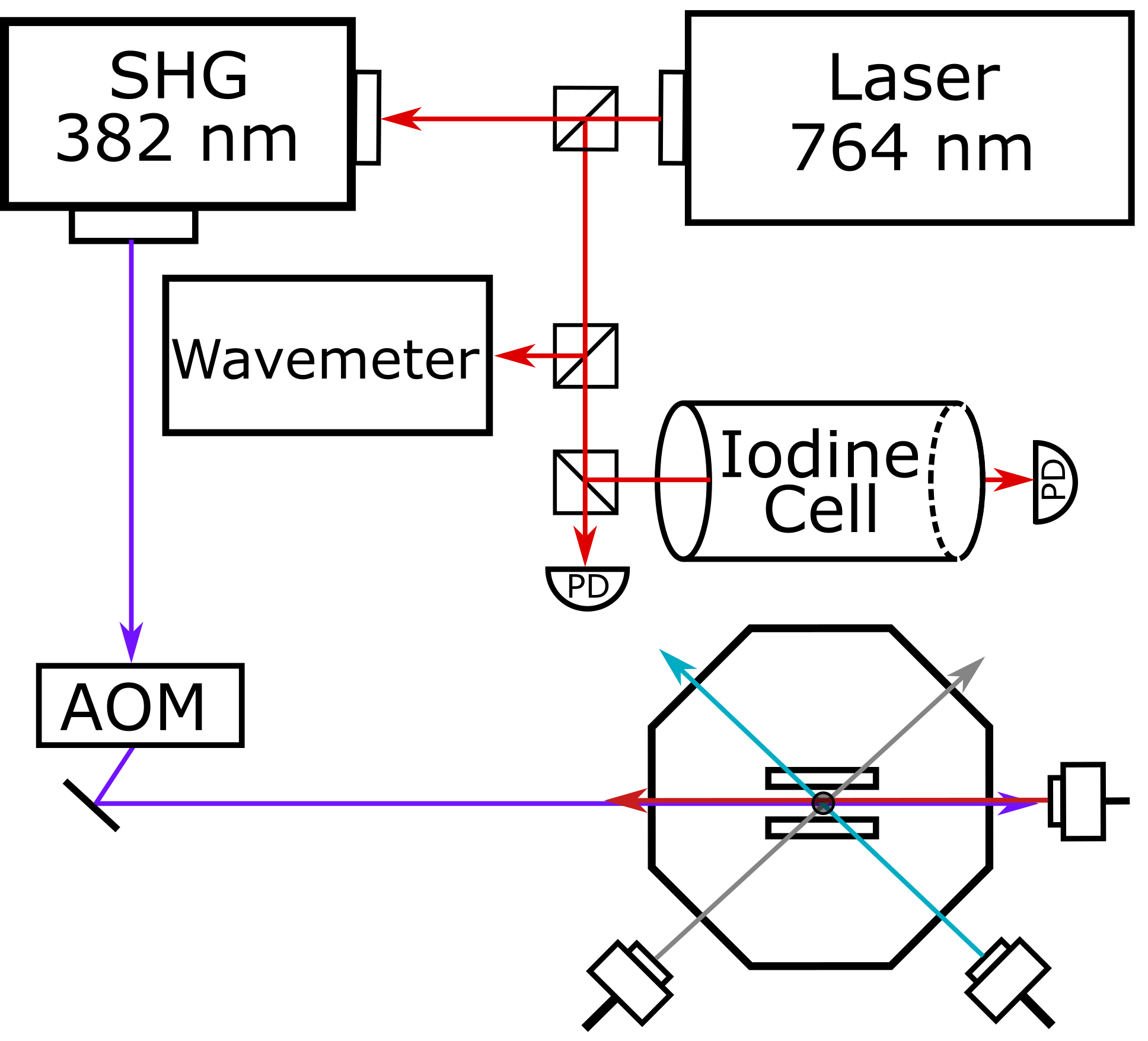
The iodine linear absorption spectrum is measured around 764 nm with light from a Ti:sapphire laser. Frequency-doubled light from the same laser drives the $S_{1/2}\rightarrow P_{3/2}$ transition of ²²⁶Ra⁺ at 382 nm (see Fig. 2). From iodine reference lines near 764 nm we can determine the $S_{1/2}\rightarrow$ $P_{3/2}$ transition frequency. During both the radium and iodine spectroscopy the 764-nm laser’s frequency is recorded with a wavemeter (High Finesse WS-8), see Fig. 3.

To measure the $S_{1/2}\rightarrow$ $P_{3/2}$ transition frequency we first scan the iodine spectrum near 764 nm, at half of the transition frequency reported in Holliman et al. 2019. We scan over a 20-GHz range that includes two iodine reference lines, 325 and 326 Gerstenkorn et al. 1982. This is followed by radium spectroscopy and then a second iodine scan to account for wavemeter drift. The radium spectroscopy uses state detection to determine if the population is in a “bright” state, $S_{1/2}$ or $D_{3/2}$, or in the $D_{5/2}$ “dark” state, by collecting Ra⁺ fluorescence at 468 nm onto a photomultiplier tube. The $S_{1/2}\rightarrow$ $P_{3/2}$ transition frequency is calculated from the difference between the radium 382-nm line center and twice the frequency of iodine line 326.

The pulse sequence for the $S_{1/2}\rightarrow P_{3/2}$ frequency measurement is shown in Fig. 4. All light is linearly polarized to drive symmetric Zeeman transitions with the same amplitude, with a 3-G magnetic field along the trap’s axial direction. We Doppler cool the ion for $500\text{\,}\mathrm{\SIUnitSymbolMicro s}$ before each pulse sequence. The initial state detection determines if the ion is cooled and if the population is in a bright state (SD1). If the population is not initialized in a bright state or if the ion is in a large orbit the data point is excluded. Population in the $D_{3/2}$ state is then optically pumped for $100\text{\,}\mathrm{\SIUnitSymbolMicro s}$ with light at 1079 nm to the ground state (P1). The $S_{1/2}\rightarrow P_{3/2}$ spectroscopy transition is then driven with light at 382 nm for $500\text{\,}\mathrm{\SIUnitSymbolMicro s}$ (P2). Decays from the $P_{3/2}$ state have an 11% probability to be shelved in the $D_{5/2}$ dark state Fan et al. 2019b. We use these decays to determine the probability of driving the $S_{1/2}\rightarrow$ $P_{3/2}$ transition at a given laser frequency with a second state detection (SD2) to form a binomial distribution, see Fig. 5. Finally, any population that remains in the $D_{5/2}$ state is reset to the bright states by optically pumping with 802 nm light (P3). The pulse sequence is repeated $32\,000\text{\,}$ times as the 382-nm laser is swept over the transition in a $\sim$$100\text{\,}\mathrm{MHz}$ range. The $S_{1/2}\rightarrow P_{3/2}$ spectroscopy is shown in Fig. 3, along with the corresponding iodine absorption reference spectrum.

The $S_{1/2}\rightarrow P_{3/2}$ radium measurement data are binned by frequency, and the shelving probability is fit to the exponential of a Lorentzian, see Fig. 5, to account for population depletion of the $S_{1/2}$ state (see Appendix A). The full width at half maximum of $40(\pm 1)\text{\,}\mathrm{MHz}$ gives a lower bound of $4.0(\pm 0.1)\text{\,}\mathrm{ns}$ for the $P_{3/2}$ state lifetime, which is in agreement with the calculated value of $4.73\text{\,}\mathrm{ns}$ Pal et al. 2009. The 382-nm light is incident on the ion along the trap’s axial direction (see Fig. 2) to minimize micromotion broadening of the transition Berkeland et al. 1998.

The closest iodine reference line to the ²²⁶Ra⁺ $S_{1/2}\rightarrow P_{3/2}$ transition is line 326 Gerstenkorn et al. 1982. We calibrate the 326 line center frequency with a wavemeter to an absolute frequency using IodineSpec5 Iod; Knöckel et al. 2004. We fit the absorption dip of line 326 in the IodineSpec5 data to a Voigt function to determine its frequency-doubled line center, $785\,734.265(\pm 0.003)\text{\,}\mathrm{GHz}$.

The frequency difference between the $S_{1/2}\rightarrow P_{3/2}$ line center at 382 nm and twice the value of the iodine line 326 center frequency is $12.16(\pm 0.03)\text{\,}\mathrm{GHz}$ (see Fig. 3). From this frequency difference we determine the $S_{1/2}\rightarrow P_{3/2}$ transition frequency to be $785\,722.11(\pm 0.03)\text{\,}\mathrm{GHz}$. The uncertainty is $\sigma_{\text{total}}=\sqrt{\sigma_{\text{Ra}^{+}}^{2}+\sigma_{\text{I}_{2}}^{2}+\sigma_{\text{spec}}^{2}+\sigma_{\text{wm}}^{2}}$, where $\sigma_{\text{Ra}^{+}}$ (20 MHz) is half the full width at half maximum of the fitted Ra⁺ spectrum (see Fig. 5) to account for possible magnetic field shifts due to Zeeman levels, $\sigma_{\text{I}_{2}}$ (10 MHz) is the iodine spectroscopy fitting uncertainty, $\sigma_{\text{spec}}$ (3 MHz) is the IodineSpec5 line uncertainty, and $\sigma_{\text{wm}}$ (20 MHz) is the wavemeter uncertainty.

This work measures a transition that was previously directly measured nearly a century ago Rasmussen 1933 and addresses a discrepancy between the frequencies reported by Nuñez, et al. Nuñez Portela et al. 2014 and by Holliman, et al. Holliman et al. 2019, see Table 1. This ²²⁶Ra⁺ frequency measurement also serves as a check for the $S_{1/2}\rightarrow D_{5/2}$ (728 nm), $S_{1/2}\rightarrow D_{3/2}$ (828 nm), $D_{3/2}\rightarrow P_{3/2}$ (708 nm), and $D_{5/2}\rightarrow P_{3/2}$ (802 nm) transition frequencies measured in Holliman et al. 2019. The $S_{1/2}\rightarrow P_{3/2}$ transition frequency can be calculated from the sum of the 728- and 802-nm frequencies, $785\,722.10(\pm 0.03)\text{\,}\mathrm{GHz}$, or the 828- and 708-nm frequencies, $785\,722.07(\pm 0.05)\text{\,}\mathrm{GHz}$. Both values derived from Holliman et al. 2019 agree with the reported direct measurement of the $S_{1/2}\rightarrow P_{3/2}$ transition frequency. We verify the self-consistency of these sets of measurements in Appendix B.

We acknowledge use of the UC Santa Barbara physics department’s Broadly-tunable Illumination Facility for Research, Outreach, Scholarship, and Training Ti:sapphire laser, which provided the 764- and 382-nm light used in this work. We also acknowledge support from NSF Grant No. PHY-1912665 and the UC Office of the President (Grant No. MRP-19-601445).

References

- Hucul et al. (2017) D. Hucul, J. E. Christensen, E. R. Hudson, and W. C. Campbell, Phys. Rev. Lett. 119, 100501 (2017).
- Fortson (1993) N. Fortson, Phys. Rev. Lett. 70, 2383 (1993).
- Berengut et al. (2018) J. C. Berengut, D. Budker, C. Delaunay, V. V. Flambaum, C. Frugiuele, E. Fuchs, C. Grojean, R. Harnik, R. Ozeri, G. Perez, and Y. Soreq, Phys. Rev. Lett. 120, 091801 (2018).
- Fan et al. (2019a) M. Fan, C. A. Holliman, A. L. Wang, and A. M. Jayich, PRL 122, 223001 (2019a).
- Sahoo et al. (2009) B. K. Sahoo, R. G. E. Timmermans, B. P. Das, and D. Mukherjee, PRA 80, 062506 (2009).
- Nuñez Portela et al. (2014) M. Nuñez Portela, E. A. Dijck, A. Mohanty, H. Bekker, J. E. van den Berg, G. S. Giri, S. Hoekstra, C. J. G. Onderwater, S. Schlesser, R. G. E. Timmermans, O. O. Versolato, L. Willmann, H. W. Wilschut, and K. Jungmann, Applied Physics B 114, 173 (2014).
- Ludlow et al. (2015) A. D. Ludlow, M. M. Boyd, J. Ye, E. Peik, and P. O. Schmidt, Rev. Mod. Phys. 87, 637 (2015).
- Heilig and Steudel (1974) K. Heilig and A. Steudel, Atomic Data and Nuclear Data Tables 14, 613 (1974).
- Reinhard et al. (2020) P.-G. Reinhard, W. Nazarewicz, and R. F. Garcia Ruiz, PRC 101, 021301(R) (2020).
- Holliman et al. (2019) C. A. Holliman, M. Fan, and A. M. Jayich, PRA 100, 062512 (2019).
- Dammalapati et al. (2016) U. Dammalapati, K. Jungmann, and L. Willmann, J. Phys. Chem. Ref. Data 45, 013101 (2016).
- Neu et al. (1989) W. Neu, R. Neugart, E. W. Otten, G. Passler, K. Wendt, B. Fricke, E. Arnold, H. J. Kluge, and G. Ulm, Zeitschrift für Physik D Atoms, Molecules and Clusters 11, 105 (1989).
- Gerstenkorn et al. (1982) S. Gerstenkorn, J. Verges, and J. Chevillard, Atlas du Spectre d’Absorption de la Molecule d’Iode: 11000-14000 cm to the Minus 1 (Laboratoire Aime-Cotton CNRS II, 1982).
- Fan et al. (2019b) M. Fan, C. A. Holliman, S. G. Porsev, M. S. Safronova, and A. M. Jayich, PRA 100, 062504 (2019b).
- Pal et al. (2009) R. Pal, D. Jiang, M. S. Safronova, and U. I. Safronova, Phys. Rev. A 79, 062505 (2009).
- Berkeland et al. (1998) D. J. Berkeland, J. D. Miller, J. C. Bergquist, W. M. Itano, and D. J. Wineland, J. Appl. Phys. 83, 5025 (1998).
- (17) H. Knöckel and E. Tiemann, IodineSpec5, (Universität Hannover, Hannover, 2011).
- Knöckel et al. (2004) H. Knöckel, B. Bodermann, and E. Tiemann, Eur. Phys. J. D 28, 199 (2004).
- Rasmussen (1933) E. Rasmussen, Zeitschrift für Physik 86, 24 (1933).
- Kramida (2011) A. Kramida, Computer Physics Communications 182, 419 (2011).