跳到论文正文
W Papers独立论文阅读器 arXiv:2008.13165 论文正文 计算阅读时间 · 0%
引用这篇论文根据当前论文元数据生成,正式投稿前建议核对。


License: arXiv.org perpetual non-exclusive license
arXiv:2008.13165v3 [math.SG] 20 Jan 2024

Multiplicative structures on cones and duality

Kai Cieliebak Address: Universität Augsburg
Universitätsstrasse 14, D-86159 Augsburg, Germany
Email address: kai.cieliebak@math.uni-augsburg.de
and Alexandru Oancea Address:  Université de Strasbourg
Institut de recherche mathématique avancée, IRMA
Strasbourg, France
Email address: oancea@unistra.fr
Date: August 11, 2026
Abstract.

We initiate the study of multiplicative structures on cones and show that cones of Floer continuation maps fit naturally in this framework. We apply this to give a new description of the multiplicative structure on Rabinowitz Floer homology and cohomology, and to give a new proof of the Poincaré duality theorem which relates the two. The underlying algebraic structure admits two incarnations, both new, which we study and compare: on the one hand the structure of A2+A_{2}^{+}-algebra on the space 𝒜\mathcal{A} of Floer chains, and on the other hand the structure of A2A_{2}-algebra involving 𝒜\mathcal{A}, its dual 𝒜∨\mathcal{A}^{\vee} and a continuation map from 𝒜∨\mathcal{A}^{\vee} to 𝒜\mathcal{A}.

1. Introduction

Rabinowitz Floer homology was originally defined as the Floer homology of the Rabinowitz action functional [7]. An alternative description as “V-shaped symplectic homology” was found in [8], relating Rabinowitz Floer homology to symplectic homology and cohomology. In [14] and [44] yet another description of Rabinowitz Floer homology was introduced, as the homology of the cone of a Floer continuation map. This proved crucial to understand its functoriality properties [14] and to extend the definition to non-exact settings [44].

Surprisingly, these three points of view are not at all equally well suited for the study of algebraic structures. Currently, the most versatile version seems to be V-shaped symplectic homology: it carries a product [14] which is a straightforward adaptation of the classical pair-of-pants product in Floer theory, and also a secondary coproduct which together with the product defines a graded Frobenius algebra structure [11]. A similar statement holds for V-shaped symplectic cohomology, the two being related by Poincaré duality [11]. A definition of such product and coproduct structures in the original setting of the Rabinowitz action functional is not available, although [1] and [18] may independently lead there.

In this paper we define and study product structures on Rabinowitz Floer homology from the perspective of cones. Besides another proof of the Poincaré duality theorem [11] in this framework, we obtain new insights into such structures that are not available by other approaches. Notions and results from this paper serve as inputs in several other articles: in [12] to relate the graded Frobenius algebra structure on Rabinowitz Floer homology of a unit cotangent bundle to that on Rabinowitz loop homology, and in [11, 16] to prove the splitting theorem for Rabinowitz Floer homology in terms of symplectic homology and cohomology. As such, this paper plays a key role in the series of articles [10, 11, 12, 13, 15, 16] on Poincaré duality for loop spaces and its applications.

Results of the paper. The cone of a chain map c:ℳ→𝒜c:\mathcal{M}\to\mathcal{A} is C​o​n​e​(c)=𝒜⊕ℳ⁡[−1]Cone(c)=\mathcal{A}\oplus\mathcal{M}[-1] with differential ∂C​o​n​e​(c)(a,x)=(∂𝒜a+c(x),−∂ℳx){\partial}_{Cone(c)}(a,x)=({\partial}_{\mathcal{A}}a+c(x),-{\partial}_{\mathcal{M}}x). In §2 we begin by spelling out the data corresponding to an A∞A_{\infty}-structure on the cone of a chain map c:ℳ→𝒜c:\mathcal{M}\to\mathcal{A} such that 𝒜⊂C​o​n​e​(c)\mathcal{A}\subset Cone(c) is an A∞A_{\infty}-subalgebra. We call such data an A∞A_{\infty}-triple. Ignoring higher homotopies, this leads to the notion of an A2A_{2}-triple (ℳ,c,𝒜)(\mathcal{M},c,\mathcal{A}). It consists of a degree 00 chain map c:ℳ→𝒜c:\mathcal{M}\to\mathcal{A} together with bilinear maps μ:𝒜⊗𝒜→𝒜\mu:\mathcal{A}\otimes\mathcal{A}\to\mathcal{A}, mL:𝒜⊗ℳ→ℳm_{L}:\mathcal{A}\otimes\mathcal{M}\to\mathcal{M}, mR:ℳ⊗𝒜→ℳm_{R}:\mathcal{M}\otimes\mathcal{A}\to\mathcal{M} of degree 00, τL:ℳ⊗𝒜→𝒜\tau_{L}:\mathcal{M}\otimes\mathcal{A}\to\mathcal{A}, τR:𝒜⊗ℳ→𝒜\tau_{R}:\mathcal{A}\otimes\mathcal{M}\to\mathcal{A}, σ:ℳ⊗ℳ→ℳ\sigma:\mathcal{M}\otimes\mathcal{M}\to\mathcal{M} of degree 11 and β:ℳ⊗ℳ→𝒜\beta:\mathcal{M}\otimes\mathcal{M}\to\mathcal{A} of degree 22 satisfying suitable relations (see Definition 2.9). In our first result we denote an element of C​o​n​e​(c)=𝒜⊕ℳ⁡[−1]Cone(c)=\mathcal{A}\oplus\mathcal{M}[-1] by (a,x¯)(a,\bar{x}), where x¯∈ℳ⁡[−1]\bar{x}\in\mathcal{M}[-1] is the shift of an element x∈ℳx\in\mathcal{M}.

Theorem A (= Propositions 2.11, 2.13 and 2.17) For an A2A_{2}-triple, the formula

m⁡((a,x¯),(a′,x¯′))\displaystyle m\big((a,\bar{x}),(a^{\prime},\bar{x}^{\prime})\big)
=(μ⁡(a,a′)+(−1)|a|​τR​(a,x′)+τL​(x,a′)−(−1)|x¯|​β​(x,x′)CLOSE,\displaystyle=\big(\mu(a,a^{\prime})+(-1)^{|a|}\tau_{R}(a,x^{\prime})+\tau_{L}(x,a^{\prime})-(-1)^{|\bar{x}|}\beta(x,x^{\prime}),
OPEN(−1)|a|​mL​(a,x′)¯+mR​(x,a′)¯−(−1)|x¯|​σ⁡(x,x′)¯)\displaystyle\qquad\qquad\qquad\qquad(-1)^{|a|}\overline{m_{L}(a,x^{\prime})}+\overline{m_{R}(x,a^{\prime})}-(-1)^{|\bar{x}|}\overline{\sigma(x,x^{\prime})}\big)

defines a degree 00 bilinear product on C​o​n​e​(c)Cone(c) which is a chain map and thus descends to homology. This product is functorial with respect to homotopy retracts and morphisms of A2A_{2}-triples.

An important part of the discussion are sign conventions related to multilinear degree shifts, tensor products, and algebraic duals, which we defer to Appendices A and B.

In §3 we apply the results of §2 to Floer theory. This is based on the observation that Floer continuation maps give rise to A∞A_{\infty}-triples which are canonically defined up to homotopy equivalence. We prove in this paper only the arity 2 version of this statement:

Theorem B (= Proposition 3.1). Floer continuation maps give rise to A2A_{2}-triples which are canonically defined up to homotopy equivalence.

The construction involves moduli spaces of solutions of Floer equations parametrized by simplices of dimension 00, 11, and 22. The construction of the A∞A_{\infty}-triple involves moduli spaces parametrized by higher dimensional simplices, much in the manner of [17], which should correspond to the assocoipahedra of Poirier and Tradler [34]. See the discussion below and Remark 7.7.

Let now WW be a Liouville domain of dimension 2​n2n with trivial canonical bundle, S​H∗SH_{*} symplectic homology graded by Conley-Zehnder indices, and S​ℍ∗=S​H∗+nS{\mathbb{H}}_{*}=SH_{*+n} its degree shifted version. The power of the cone perspective derives from its applicability to various families of Floer continuation maps. Applying the construction of a product on the cone to the three families of Floer continuation maps {Kλ}\{K_{\lambda}\}, ℋ∨\mathcal{H}_{\vee} and ℋ∧\mathcal{H}_{\wedge} shown in Figure 1 gives rise to three rings S​ℍ∗​({Kλ})S{\mathbb{H}}_{*}(\{K_{\lambda}\}), S​ℍ∗​(ℋ∨)S{\mathbb{H}}_{*}(\mathcal{H}_{\vee}) and S​ℍ∗​(ℋ∧)S{\mathbb{H}}_{*}(\mathcal{H}_{\wedge}).

Refer to caption
Figure 1. The families of Floer continuation maps {Kλ}\{K_{\lambda}\}, ℋ∨\mathcal{H}_{\vee} and ℋ∧\mathcal{H}_{\wedge}.

The first two of these recover Rabinowitz Floer homology S​ℍ∗​(∂W)S{\mathbb{H}}_{*}({\partial}W) with its product defined in [11]:

Theorem C. We have canonical ring isomorphisms

S​ℍ∗​({Kλ})≃S​ℍ∗​(ℋ∨)≃S​ℍ∗​(∂W).S{\mathbb{H}}_{*}(\{K_{\lambda}\})\simeq S{\mathbb{H}}_{*}(\mathcal{H}_{\vee})\simeq S{\mathbb{H}}_{*}({\partial}W).

The third one corresponds to Rabinowitz Floer cohomology SH1−n−∗(∂W)SH^{1-n-*}({\partial}W) with its product defined in [11]:

Theorem D. We have canonical ring isomorphisms

Sℍ∗(ℋ∧)≃S​H^∗+n−1(∂W)≃SH1−n−∗(∂W).S{\mathbb{H}}_{*}(\mathcal{H}_{\wedge})\simeq\widehat{SH}_{*+n-1}({\partial}W)\simeq SH^{1-n-*}({\partial}W).

Here S​H^∗​(∂W)=S​H∗​(V,∂V)\widehat{SH}_{*}({\partial}W)=SH_{*}(V,{\partial}V) for the symplectic cobordism V=[0,1]×∂WV=[0,1]\times{\partial}W in the terminology of [14]. In §4.2 and §4.3 we give direct definitions of the product and its unit on S​H^∗+n−1​(∂W)\widehat{SH}_{*+n-1}({\partial}W), and thus on Rabinowitz Floer cohomology.

Theorem E (Cone duality). There is a canonical ring isomorphism

S​ℍ∗​(ℋ∨)≃S​ℍ∗​(ℋ∧).S{\mathbb{H}}_{*}(\mathcal{H}_{\vee})\simeq S{\mathbb{H}}_{*}(\mathcal{H}_{\wedge}).

The above ring isomorphisms are summarized in the following diagram:

SH1−n−∗(∂W)\textstyle{SH^{1-n-*}({\partial}W)\ignorespaces\ignorespaces\ignorespaces\ignorespaces\ignorespaces\ignorespaces\ignorespaces\ignorespaces}Thm. 4.1  Prop. 5.6S​ℍ∗​(∂W)\textstyle{S{\mathbb{H}}_{*}({\partial}W)\ignorespaces\ignorespaces\ignorespaces\ignorespaces\ignorespaces\ignorespaces\ignorespaces\ignorespaces}Thm. 4.2Thm. 5.2S​H^∗+n−1​(∂W)\textstyle{\widehat{SH}_{*+n-1}({\partial}W)\ignorespaces\ignorespaces\ignorespaces\ignorespaces}Thm. 5.4S​ℍ∗​(ℋ∨)\textstyle{S{\mathbb{H}}_{*}(\mathcal{H}_{\vee})\ignorespaces\ignorespaces\ignorespaces\ignorespaces\ignorespaces\ignorespaces\ignorespaces\ignorespaces}Thm. 4.2Thm. 5.1S​ℍ∗​(ℋ∧)\textstyle{S{\mathbb{H}}_{*}(\mathcal{H}_{\wedge})}S​ℍ∗​({Kλ})\textstyle{S{\mathbb{H}}_{*}(\{K_{\lambda}\})}

Theorems C, D and E together give a new proof of the Poincaré duality theorem from [11] (which we restate in this paper as Theorem 4.1). Moreover, the preceding theorems are crucial inputs for the proof of the splitting theorem for Rabinowitz Floer homology ([16, Proposition 7.6] and [11, Theorem 1.5]). In turn, this splitting theorem serves as a computational tool for the multiplicative structure on Rabinowitz Floer homology, see [16, Theorem 7.8] and [11, §2].

The explicit description of the product on S​H^∗+n−1​(∂W)\widehat{SH}_{*+n-1}({\partial}W) allows us to relate it to the varying weights secondary product, originally constructed by Seidel and further explored in [17, 2]:

Theorem F (= Proposition 6.2). On negative action symplectic homology S​H^∗+n−1<0(∂W)≃SH>01−n−∗(∂W)\widehat{SH}_{*+n-1}^{<0}({\partial}W)\simeq SH^{1-n-*}_{>0}({\partial}W) the product in Theorem D agrees with the varying weights secondary product.

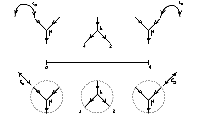
Rabinowitz Floer homology arises from an A2A_{2}-triple (ℳ,c,𝒜)(\mathcal{M},c,\mathcal{A}) in which ℳ\mathcal{M} is the algebraic dual 𝒜∨\mathcal{A}^{\vee} of 𝒜\mathcal{A}. This allows one to encode all the structure on 𝒜\mathcal{A} alone. We formalize this in §7 in the notion of an A2+A_{2}^{+}-structure on 𝒜\mathcal{A}. It consists of a degree 00 copairing c0∈𝒜⊗𝒜c_{0}\in\mathcal{A}\otimes\mathcal{A}, a degree 11 secondary copairing Q0∈𝒜⊗𝒜Q_{0}\in\mathcal{A}\otimes\mathcal{A}, a degree 00 product μ:𝒜⊗𝒜→𝒜\mu:\mathcal{A}\otimes\mathcal{A}\to\mathcal{A}, a degree 11 secondary coproduct λ:𝒜→𝒜⊗𝒜\lambda:\mathcal{A}\to\mathcal{A}\otimes\mathcal{A} and a degree 22 cubic vector B∈𝒜⊗𝒜⊗𝒜B\in\mathcal{A}\otimes\mathcal{A}\otimes\mathcal{A} satisfying suitable relations (see Definition 7.1).

Theorem G (= Propositions 7.6 and 7.11). An A2+A_{2}^{+}-structure on 𝒜\mathcal{A} gives rise to an A2A_{2}-triple (𝒜∨,c,𝒜)(\mathcal{A}^{\vee},c,\mathcal{A}), and a morphism of A2+A_{2}^{+}-algebras gives rise to a correspondence of A2A_{2}-triples.

As a consequence, a quasi-isomorphism of A2+A_{2}^{+}-algebras induces a ring isomorphism between the homologies of the cones (Corollary 7.12). This result is a crucial input for the proof of the Frobenius algebra isomorphism between Rabinowitz Floer homology of a unit cotangent bundle and Rabinowitz loop homology in [12]. Here the difficulty lies in the fact that Rabinowitz homology is an amalgamation of homology and cohomology, which are covariant resp. contravariant under the Viterbo isomorphism. It is overcome by encoding the whole structure as an A2+A_{2}^{+}-structure on homology alone and using its functoriality above.

Since the notion of an A2+A_{2}^{+}-structure is self-dual, in addition to a product 𝝁\bm{\mu} it also induces a coproduct 𝝀\bm{\lambda} on its cone. This product and coproduct can be read as a coproduct 𝝁∨\bm{\mu}^{\vee} and product 𝝀∨\bm{\lambda}^{\vee} on the dual of the cone. The following result can be viewed as an algebraic counterpart of the Poincaré Duality Theorem in [11].

Theorem H (Duality for A2+A_{2}^{+}-algebras) (= Theorem 7.14). Let 𝒜\mathcal{A} be an A2+A_{2}^{+}-algebra which is free and finite dimensional in each degree. Then we have a canonical isomorphism

(H∗​(C​o​n​e​(c)),𝝁,𝝀)≅(H∗−1​(C​o​n​e​(c)∨),𝝀∨​τ,τ​𝝁∨)\Bigl(H_{*}\bigl(Cone(c)\bigr),\bm{\mu},\bm{\lambda}\Bigr)\cong\Bigl(H_{*-1}\bigl(Cone(c)^{\vee}\bigr),\bm{\lambda}^{\vee}\tau,\tau\bm{\mu}^{\vee}\Bigr)

intertwining the products and coproducts, where τ\tau is the map flipping the tensor factors with signs.

Extensions. The results in this paper have several straightforward extensions. (a) In this paper we treat explicitly only products, but there is an entirely parallel discussion of coproducts. (b) Sara Venkatesh defined in [44] Rabinowitz Floer homology in non-exact settings as the cone of such a continuation map at the additive level. The perspective on multiplicative structures that we adopt here is robust and would carry over to such situations. (c) We formulate all our results for closed strings, in terms of symplectic homology, but they have natural open string counterparts with Lagangian boundary conditions in terms of wrapped Floer homology. See [14, 11] for a discussion of such extensions, in particular regarding the gradings.

Relation to other work and future directions. The notion of an A2+A_{2}^{+}-algebra encodes only operations with up to 33 inputs and outputs, which suffices for our applications on the level of homology. Considering Floer moduli spaces with more inputs and outputs leads to a homotopical version of an A2+A_{2}^{+}-algebra, which we may call an “A∞+A_{\infty}^{+}-algebra”. Special cases of this structure have appeared in the literature under various names: V∞V_{\infty}-algebras in Tradler–Zeinalian [42], double Poisson algebras in Van den Bergh [43], and pre-Calabi-Yau algebras in Iyudu–Kontsevich–Vlassopoulos [22] and Kontsevich-Takeda-Vlassopoulos [25]. In fact, Leray and Vallette have proved that curved versions of these three structures are equivalent [28]. The presence of the copairing c0c_{0} in Definition 7.1 means that our structure is also curved. What distinguishes it from the other structures is the presence of the secondary copairing Q0Q_{0} which measures the failure of c0c_{0} to be symmetric. This is dictated to us by the applications in symplectic homology and string topology, where a nontrivial Q0Q_{0} occurs and is responsible for various subtleties concerning the algebraic structure on reduced homology [16].

Poirier and Tradler have shown that the dioperad V∞V_{\infty} is governed by a family of polytopes called “assocoipahedra” [34, 35]. In view of the preceding discussion, we expect that these can be realized as Floer moduli spaces in the absence of Q0Q_{0}. This connection was first proposed by T. Mazuir after observing the equivalence of Figure 7 in [16] with Figure 9 in [34]. It is an interesting challenge to find polyhedral descriptions of the Floer moduli spaces in the presence of Q0Q_{0} and study the resulting dioperad.

It is proved in [11] that Rabinowitz Floer homology of the boundary of a Liouville domain carries the structure of a graded Frobenius algebra. This structure emanates from the cone description of Rabinowitz Floer homology if we enhance the underlying A2+A_{2}^{+}-algebra to include operations with 44 inputs and outputs. Based on this, we conjecture that an A∞+A_{\infty}^{+}-algebra gives rise to a homotopy version of a graded Frobenius algebra on its cone. The development of this homotopy theory is the subject of ongoing work by Mazuir [31].

It has long been observed that the definition of Rabinowitz Floer homology resembles that of Tate homology, see e.g. [4] for an application of this point of view in equivariant homology. We conjecture that our Poincaré Duality Theorem 4.1 is an instantiation of Tate duality and we intend to explore this in future work. For cotangent bundles of simply connected manifolds, the structure we find on Rabinowitz Floer homology should coincide with the structure found by Rivera and Wang [37] on singular Hochschild cohomology of the dga of cochains. Our work should also be related to earlier work of Kaufmann such as [23], and to Kontsevich graph complexes as studied by Merkulov–Willwacher [32].

In the closed string case, Rabinowitz Floer homology also carries a natural BV operator, see [13]. To complete the algebraic picture, one should therefore incorporate BV-structures in the formalisms developed in this paper. The S1S^{1}-equivariant versions of these structures should give rise to a refinement of the IBL∞{\rm IBL}_{\infty} structures from [9].

The wrapped Floer homology groups have a categorical refinement given by the wrapped Fukaya category [3]. Recently Ganatra-Gao-Venkatesh [20] and Bae-Jeong-Kim [5] have defined a categorical refinement of the Lagrangian Rabinowitz Floer homology groups called Rabinowitz Fukaya category. The cone perspective on Rabinowitz Floer homology plays a key role, and it is an interesting question to compare the moduli spaces used in those constructions with the moduli spaces from this paper. In [5] it is proved that, under reasonable assumptions, the Rabinowitz Fukaya category of a Liouville domain of dimension 2​n2n is (n−1)(n-1)-Calabi-Yau. This raises the question whether, and how, such a statement implies our Poincaré duality theorem. Legout [27] had previously defined a categorical refinement of the Cthulhu homology of Chantraine-Dimitroglou Rizell-Ghiggini-Golovko [6], in the setting of Lagrangian cobordisms. We conjecture that, when transposed to the context of Liouville domains, the Legout category is equivalent to the Rabinowitz Fukaya category.

Acknowledgements. This paper is a split-off from our collaboration with Nancy Hingston on Poincaré duality. Without her far reaching vision this could not have come into being. The authors benefited from discussions with M. Abouzaid, B. Chantraine, F. Chapoton, V. Dotsenko, P. Ghiggini, R. Kaufmann, T. Mazuir, M. Rivera, and S. Venkatesh. The first author thanks Stanford University, Institut Mittag–Leffler, and the Institute for Advanced Study for their hospitality over the duration of this project. The second author acknowledges the hospitality of Helmut Hofer and IAS in 2017, 2019, and 2022.

This work has benefited from financial support via the grants MICROLOCAL ANR-15-CE40-0007, ENUMGEOM ANR-18-CE40-0009 and COSY ANR-21-CE40-0002. In its late stages, it has also benefited from support provided to the second author by the University of Strasbourg Institute for Advanced Study (USIAS) for a Fellowship, within the French national programme “Investment for the future” (IdEx-Unistra).

2. Products on cones

Throughout this section we use homological conventions and coefficients in a principal ideal domain RR. Recall that, given a degree 00 chain map c:ℳ∗→𝒜∗c:\mathcal{M}_{*}\to\mathcal{A}_{*} between chain complexes whose differentials have degree −1-1, the cone of a chain map c:ℳ→𝒜c:\mathcal{M}\to\mathcal{A} is the chain complex

Cone(c)=𝒜⊕ℳ[−1],∂C​o​n​e​(c)=(∂𝒜c0−∂ℳ)Cone(c)=\mathcal{A}\oplus\mathcal{M}[-1],\qquad{\partial}_{Cone(c)}=\begin{pmatrix}{\partial}_{\mathcal{A}}&c\\ 0&-{\partial}_{\mathcal{M}}\end{pmatrix}

with ℳ​[−1]∗=ℳ∗−1\mathcal{M}[-1]_{*}=\mathcal{M}_{*-1} and ∂ℳ⁡[−1]=−∂ℳ{\partial}_{\mathcal{M}[-1]}=-{\partial}_{\mathcal{M}}. The inclusion 𝒜↪C​o​n​e​(c)\mathcal{A}\hookrightarrow Cone(c), a↦(a,0)a\mapsto(a,0) is a chain map. We shall freely refer in this section to the notation of Appendix A regarding degree shifts in the multilinear setting.

Definition 2.1.

An A∞A_{\infty}-algebra 𝒜\mathcal{A} is a ℤ{\mathbb{Z}}-graded RR-module endowed with a collection of maps μ𝒜d:𝒜​[−1]⊗d→𝒜⁡[−1]\mu^{d}_{\mathcal{A}}:\mathcal{A}[-1]^{\otimes d}\to\mathcal{A}[-1], d≥1d\geq 1 of degree −1-1 satisfying the relations

∑i+j=k+1∑t=1iμ𝒜i​(1​l⊗t−1⊗μ𝒜j⊗1​l⊗i−t)=0,k≥1.\sum_{i+j=k+1}\sum_{t=1}^{i}\mu^{i}_{\mathcal{A}}({{\mathchoice{\mathrm{1\mskip-4.0mul}}{\mathrm{1\mskip-4.0mul}}{\mathrm{1\mskip-4.5mul}}{\mathrm{1\mskip-5.0mul}}}}^{\otimes\,t-1}\otimes\mu^{j}_{\mathcal{A}}\otimes{{\mathchoice{\mathrm{1\mskip-4.0mul}}{\mathrm{1\mskip-4.0mul}}{\mathrm{1\mskip-4.5mul}}{\mathrm{1\mskip-5.0mul}}}}^{\otimes\,i-t})=0,\qquad k\geq 1. (1)

In the absence of the shift the structure maps μ𝒜d:𝒜⊗d→𝒜\mu^{d}_{\mathcal{A}}:\mathcal{A}^{\otimes d}\to\mathcal{A} have degree d−2d-2. The functional relation translates by evaluation into the relation

∑i+j=k+1∑t=1i\displaystyle\sum_{i+j=k+1}\sum_{t=1}^{i} (−1)‖a1‖+⋯+‖at−1‖\displaystyle(-1)^{\|a_{1}\|+\dots+\|a_{t-1}\|}
μ𝒜i​(a1,…,at−1,μ𝒜j​(at,…,at+j−1),at+j,…​ai)=0,k≥1,\displaystyle\mu^{i}_{\mathcal{A}}(a_{1},\dots,a_{t-1},\mu^{j}_{\mathcal{A}}(a_{t},\dots,a_{t+j-1}),a_{t+j},\dots a_{i})=0,\quad k\geq 1,

where ‖a‖=|a|+1\|a\|=|a|+1 denotes the shifted degree. The data of an A∞A_{\infty}-algebra on a ℤ{\mathbb{Z}}-graded RR-module 𝒜\mathcal{A} is equivalent to the data of a square-zero coderivation on T¯c(𝒜[−1])=⊕k≥1𝒜[−1]⊗k{\overline{T}}^{c}(\mathcal{A}[-1])=\oplus_{k\geq 1}\mathcal{A}[-1]^{\otimes k}, the reduced tensor coalgebra on 𝒜⁡[−1]\mathcal{A}[-1]. This is because each μ𝒜d\mu^{d}_{\mathcal{A}} can be uniquely extended as a coderivation μ¯𝒜d:T¯c​(𝒜⁡[−1])→T¯c​(𝒜⁡[−1])\overline{\mu}^{d}_{\mathcal{A}}:\overline{T}^{c}(\mathcal{A}[-1])\to\overline{T}^{c}(\mathcal{A}[-1]) and, setting μ¯𝒜=∑dμ¯𝒜d\overline{\mu}_{\mathcal{A}}=\sum_{d}\overline{\mu}^{d}_{\mathcal{A}}, the A∞A_{\infty}-relations are equivalent to μ¯𝒜∘μ¯𝒜=0\overline{\mu}_{\mathcal{A}}\circ\overline{\mu}_{\mathcal{A}}=0.

Definition 2.2.

Given two A∞A_{\infty}-algebras 𝒜\mathcal{A} and 𝒜′\mathcal{A}^{\prime}, an A∞A_{\infty}-morphism ℱ:𝒜→𝒜′\mathcal{F}:\mathcal{A}\to\mathcal{A}^{\prime} is a collection of maps ℱd:𝒜​[−1]⊗d→𝒜′​[−1]\mathcal{F}^{d}:\mathcal{A}[-1]^{\otimes d}\to\mathcal{A}^{\prime}[-1], d≥1d\geq 1 of degree 00 which satisfy the relations

∑i=1d∑j,k,ℓℱi​(1​l⊗j⊗μ𝒜k⊗1​l⊗ℓ)=∑r∑i1,…,irμ𝒜′r​(ℱi1⊗⋯⊗ℱir),d≥1.\sum_{i=1}^{d}\sum_{j,k,\ell}\mathcal{F}^{i}({{\mathchoice{\mathrm{1\mskip-4.0mul}}{\mathrm{1\mskip-4.0mul}}{\mathrm{1\mskip-4.5mul}}{\mathrm{1\mskip-5.0mul}}}}^{\otimes\,j}\otimes\mu_{\mathcal{A}}^{k}\otimes{{\mathchoice{\mathrm{1\mskip-4.0mul}}{\mathrm{1\mskip-4.0mul}}{\mathrm{1\mskip-4.5mul}}{\mathrm{1\mskip-5.0mul}}}}^{\otimes\,\ell})=\sum_{r}\sum_{i_{1},\dots,i_{r}}\mu_{\mathcal{A}^{\prime}}^{r}(\mathcal{F}^{i_{1}}\otimes\dots\otimes\mathcal{F}^{i_{r}}),\quad d\geq 1. (2)

The data of the collection {ℱd}\{\mathcal{F}^{d}\} is equivalent to the data of a chain map ℱ¯:(T¯c​(𝒜⁡[−1]),μ¯𝒜)→(T¯c​(𝒜′​[−1]),μ¯𝒜′)\overline{\mathcal{F}}:({\overline{T}}^{c}(\mathcal{A}[-1]),\overline{\mu}_{\mathcal{A}})\to({\overline{T}}^{c}(\mathcal{A}^{\prime}[-1]),\overline{\mu}_{\mathcal{A}^{\prime}}), i.e. ℱ¯∘μ¯𝒜=μ¯𝒜′∘ℱ¯\overline{\mathcal{F}}\circ\overline{\mu}_{\mathcal{A}}=\overline{\mu}_{\mathcal{A}^{\prime}}\circ\overline{\mathcal{F}}.

If μ𝒜d=0\mu^{d}_{\mathcal{A}}=0 for d>2d>2 the A∞A_{\infty}-structure determines a dga structure on 𝒜\mathcal{A} by the formulas

∂𝒜\displaystyle{\partial}_{\mathcal{A}} =−μ𝒜1=μ𝒜1​[1],\displaystyle=-\mu^{1}_{\mathcal{A}}=\mu^{1}_{\mathcal{A}}[1], (3)
a⋅a′\displaystyle a\cdot a^{\prime} =(−1)|a|​μ𝒜2​(a,a′)=μ𝒜2​[1,1;1]​(a,a′).\displaystyle=(-1)^{|a|}\mu^{2}_{\mathcal{A}}(a,a^{\prime})=\mu^{2}_{\mathcal{A}}[1,1;1](a,a^{\prime}). (4)

See Appendix A for an explanation of the notation μ𝒜2​[1,1;1]\mu^{2}_{\mathcal{A}}[1,1;1]. In the case where μ𝒜d=0\mu^{d}_{\mathcal{A}}=0 for d>3d>3 the same formulas determine an associative-up-to-homotopy differential graded algebra structure on 𝒜\mathcal{A}. More precisely, with h⁡(a1,a2,a3)=(−1)|a2|​μ𝒜3​(a1,a2,a3)h(a_{1},a_{2},a_{3})=(-1)^{|a_{2}|}\mu^{3}_{\mathcal{A}}(a_{1},a_{2},a_{3}), i.e. h=μ𝒜3​[1,1,1;1]h=\mu^{3}_{\mathcal{A}}[1,1,1;1] in the notation of Appendix A, we have 11 1 The conventions for the definition of an A∞A_{\infty}-algebra vary greatly throughout the literature, and the difference stems mainly from the point of view adopted: either square-zero coderivation on T¯c​(𝒜​[−1])\overline{T}^{c}(\mathcal{A}[-1]), or homotopy relaxation of dga structure. All conventions are equivalent to one another by suitable sign changes, and the short note by Polishchuk [36] contains a useful comparison. Our convention derives the functional relation (1), which involves no signs, from the condition that the associated coderivation on the reduced tensor coalgebra on 𝒜⁡[−1]\mathcal{A}[-1] squares to zero. This is the point of view of Fukaya-Oh-Ohta-Ono [19, Definition 3.2.3] and Seidel [(2.1)][39]. Seidel’s convention in [40, (1.2)] is essentially the same except that the maps μ𝒜d\mu^{d}_{\mathcal{A}} are viewed as acting from the right, so one passes from one convention to the other by defining μ~𝒜d​(ad,…,a1)=μ𝒜d​(a1,…,ad)\tilde{\mu}^{d}_{\mathcal{A}}(a_{d},\dots,a_{1})=\mu^{d}_{\mathcal{A}}(a_{1},\dots,a_{d}). The conventions of Lefèvre-Hasegawa [26, 1.2.1.1] and Markl [30, (2)], which coincide, are such that the first three structure maps directly define on 𝒜\mathcal{A} an associative-up-to-homotopy differential graded algebra structure. They are the same as the original one of Stasheff [41], cf. [36]. Lefèvre-Hasegawa writes down in [26, Lemma 1.2.2.1] a transformation through which this point of view is equivalent to ours, and that transformation inspired our treatment of shifts in Appendix A. The conventions by which one associates to an A∞A_{\infty}-algebra in the sense of Definition 2.1 an associative-up-to-homotopy dga structure vary greatly as well. Ours is different from both the one of Fukaya-Oh-Ohta-Ono [19, (3.2.5)] and the one of Seidel [40, (1.3)]. We favour it because it fits into a systematic procedure of shifting multilinear maps, cf. Appendix A, and also because it realizes (𝒜,∂𝒜)(\mathcal{A},{\partial}_{\mathcal{A}}) as the shift of (𝒜⁡[−1],μ𝒜1)(\mathcal{A}[-1],\mu^{1}_{\mathcal{A}}).

(a1⋅a2)⋅a3−a1⋅(a2⋅a3)=[∂𝒜,h].(a_{1}\cdot a_{2})\cdot a_{3}-a_{1}\cdot(a_{2}\cdot a_{3})=[{\partial}_{\mathcal{A}},h]. (5)

Similarly, given an A∞A_{\infty}-morphism ℱ:𝒜→𝒜′\mathcal{F}:\mathcal{A}\to\mathcal{A}^{\prime} the map f=ℱ1​[1;1]:𝒜→𝒜′f=\mathcal{F}^{1}[1;1]:\mathcal{A}\to\mathcal{A}^{\prime} acts on elements as f​(a)=ℱ1​(a)f(a)=\mathcal{F}^{1}(a) and is a chain map which intertwines the products m𝒜=μ𝒜2​[1,1;1]m_{\mathcal{A}}=\mu^{2}_{\mathcal{A}}[1,1;1] and m𝒜′=μ𝒜′2​[1,1;1]m_{\mathcal{A}^{\prime}}=\mu^{2}_{\mathcal{A}^{\prime}}[1,1;1] on 𝒜\mathcal{A} and 𝒜′\mathcal{A}^{\prime} up to a homotopy k=ℱ2​[1,1;1]k=\mathcal{F}^{2}[1,1;1], i.e.

m𝒜′(f⊗f)−fm𝒜=[∂,k].m_{\mathcal{A}^{\prime}}(f\otimes f)-fm_{\mathcal{A}}=[{\partial},k].

Our discussion evolves around the following refinement of the notion of an A∞A_{\infty}-algebra and A∞A_{\infty}-morphism.

Definition 2.3.

An A∞A_{\infty}-triple (ℳ,c,𝒜)(\mathcal{M},c,\mathcal{A}) consists of an A∞A_{\infty}-algebra 𝒜\mathcal{A}, a chain complex ℳ\mathcal{M} and a degree 00 chain map

c:ℳ→𝒜,c:\mathcal{M}\to\mathcal{A},

together with an A∞A_{\infty}-algebra structure on C​o​n​e​(c)Cone(c) extending the A∞A_{\infty}-algebra structure on 𝒜\mathcal{A} via the inclusion 𝒜↪C​o​n​e​(c)=𝒜⊕ℳ⁡[−1]\mathcal{A}\hookrightarrow Cone(c)=\mathcal{A}\oplus\mathcal{M}[-1], and such that μC​o​n​e​(c)1=∂C​o​n​e​(c)[−1]\mu^{1}_{Cone(c)}={\partial}_{Cone(c)}[-1].

Definition 2.4.

An A∞A_{\infty}-morphism ℱ:(ℳ,c,𝒜)→(ℳ′,c′,𝒜′)\mathcal{F}:(\mathcal{M},c,\mathcal{A})\to(\mathcal{M}^{\prime},c^{\prime},\mathcal{A}^{\prime}) between A∞A_{\infty}-triples is an A∞A_{\infty}-morphism C​o​n​e​(c)→C​o​n​e​(c′)Cone(c)\to Cone(c^{\prime}) which restricts to an A∞A_{\infty}-morphism 𝒜→𝒜′\mathcal{A}\to\mathcal{A}^{\prime}.

2.1. The point of view of split pairs of A∞A_{\infty}-algebras

The data of an A∞A_{\infty}-triple is equivalent to the data of an RR-split pair of A∞A_{\infty}-algebras, or simply split pair of A∞A_{\infty}-algebras, meaning an inclusion of A∞A_{\infty}-algebras 𝒜⊂ℬ\mathcal{A}\subset\mathcal{B} together with a splitting (as graded RR-modules) s:ℬ/𝒜→ℬs:\mathcal{B}/\mathcal{A}\to\mathcal{B} of the short exact sequence 0→𝒜→ℬ→ℬ/𝒜→00\to\mathcal{A}\to\mathcal{B}\to\mathcal{B}/\mathcal{A}\to 0. Given such a pair we write the differential on ℬ\mathcal{B} in upper triangular form with respect to the decomposition ℬ=𝒜⊕(ℬ/𝒜)\mathcal{B}=\mathcal{A}\oplus(\mathcal{B}/\mathcal{A}) induced by the splitting, we set ℳ=(ℬ/𝒜)​[1]\mathcal{M}=(\mathcal{B}/\mathcal{A})[1] and we define c:ℳ→𝒜c:\mathcal{M}\to\mathcal{A} to be the (ℬ/𝒜,𝒜)(\mathcal{B}/\mathcal{A},\mathcal{A})-component of the differential. Then there is an induced structure of A∞A_{\infty}-triple on (ℳ,c,𝒜)(\mathcal{M},c,\mathcal{A}) such that C​o​n​e​(c)=ℬCone(c)=\mathcal{B}. Conversely, given an A∞A_{\infty}-triple (ℳ,c,𝒜)(\mathcal{M},c,\mathcal{A}) the inclusion 𝒜⊂C​o​n​e​(c)\mathcal{A}\subset Cone(c) is obviously split.

The key property of A∞A_{\infty}-structures is that they obey the Homotopy Transfer Theorem, see [30] for its most general form and [29, §9.4] for a contextual discussion. In the context of split pairs of A∞A_{\infty}-algebras 𝒜⊂ℬ\mathcal{A}\subset\mathcal{B} the homotopy transfer theorem adapts in an obvious way by considering only maps which are upper triangular with respect to the decomposition ℬ=𝒜⊕ℬ/𝒜\mathcal{B}=\mathcal{A}\oplus\mathcal{B}/\mathcal{A} provided by the splitting.

Definition 2.5.

Let 𝒜⊂ℬ\mathcal{A}\subset\mathcal{B} and 𝒜′⊂ℬ′\mathcal{A}^{\prime}\subset\mathcal{B}^{\prime} be split pairs of chain complexes. We say that the pair 𝒜′⊂ℬ′\mathcal{A}^{\prime}\subset\mathcal{B}^{\prime} is a homotopy retract of the pair 𝒜⊂ℬ\mathcal{A}\subset\mathcal{B} if there are maps

ℬ{\lx@inpgf@ignorespaces\mathcal{B}}ℬ′{\lx@inpgf@ignorespaces\mathcal{B}^{\prime}}H\scriptstyle{\lx@inpgf@ignorespaces H}P\scriptstyle{\lx@inpgf@ignorespaces P}I\scriptstyle{\lx@inpgf@ignorespaces I}

which are upper triangular with respect to the decompositions ℬ=𝒜⊕ℬ/𝒜\mathcal{B}=\mathcal{A}\oplus\mathcal{B}/\mathcal{A} and ℬ′=𝒜′⊕ℬ′/𝒜′\mathcal{B}^{\prime}=\mathcal{A}^{\prime}\oplus\mathcal{B}^{\prime}/\mathcal{A}^{\prime} provided by the splittings and such that

[∂,H]=1l−IP.[{\partial},H]={{\mathchoice{\mathrm{1\mskip-4.0mul}}{\mathrm{1\mskip-4.0mul}}{\mathrm{1\mskip-4.5mul}}{\mathrm{1\mskip-5.0mul}}}}-IP.

The proof of the next theorem is the same as that of [30, Theorem 5]. It specifically uses the upper triangular form of the maps P,I,HP,I,H, and also the explicit formulas provided by Markl in [30].

Theorem 2.6 (Homotopy transfer for split pairs).

Given a homotopy retraction of pairs as above, and given an A∞A_{\infty}-algebra structure on ℬ\mathcal{B} such that 𝒜\mathcal{A} is a subalgebra, there is an A∞A_{\infty}-structure on ℬ′\mathcal{B}^{\prime} such that 𝒜′\mathcal{A}^{\prime} is a subalgebra, and there are extensions of P,IP,I to A∞A_{\infty}-morphisms of pairs P~,I~\tilde{P},\tilde{I} and of HH to an A∞A_{\infty}-homotopy H~\tilde{H} between I~​P~\tilde{I}\tilde{P} and 1​l{{\mathchoice{\mathrm{1\mskip-4.0mul}}{\mathrm{1\mskip-4.0mul}}{\mathrm{1\mskip-4.5mul}}{\mathrm{1\mskip-5.0mul}}}} which preserves 𝒜\mathcal{A}. ∎

The transferred A∞A_{\infty}-structure and the extensions P~,I~,H~\tilde{P},\tilde{I},\tilde{H} are described very explicitly in terms of summation over trees whose vertices are at least trivalent, see [30] and also [24].

One particularly relevant situation is that in which the maps P,IP,I defining a homotopy retract are actually homotopy inverses, with the homotopy H′:ℬ′→ℬ′H^{\prime}:\mathcal{B}^{\prime}\to\mathcal{B}^{\prime} such that [∂,H′]=1l−PI[{\partial},H^{\prime}]={{\mathchoice{\mathrm{1\mskip-4.0mul}}{\mathrm{1\mskip-4.0mul}}{\mathrm{1\mskip-4.5mul}}{\mathrm{1\mskip-5.0mul}}}}-PI being also in upper triangular form. The next result is the analogue of [30, Proposition 12].

Proposition 2.7.

In the preceding situation, the homotopy H′H^{\prime} can be extended to an A∞A_{\infty}-homotopy H~′\tilde{H}^{\prime} between P~​I~\tilde{P}\tilde{I} and 1​l{{\mathchoice{\mathrm{1\mskip-4.0mul}}{\mathrm{1\mskip-4.0mul}}{\mathrm{1\mskip-4.5mul}}{\mathrm{1\mskip-5.0mul}}}} which preserves 𝒜\mathcal{A} if

[P​H−H′​P]=0∈H1​(H​o​m​(ℬ,ℬ′)),[PH-H^{\prime}P]=0\in H_{1}(Hom(\mathcal{B},\mathcal{B}^{\prime})),

and P​H−H′​PPH-H^{\prime}P admits a primitive which is upper triangular. ∎

2.2. The point of view of A∞A_{\infty}-bimodules

Recall that an A∞A_{\infty}-algebra ℬ\mathcal{B} is a graded RR-module with operations μℬd:ℬ​[−1]⊗d→ℬ⁡[−1]\mu^{d}_{\mathcal{B}}:\mathcal{B}[-1]^{\otimes d}\to\mathcal{B}[-1], d≥1d\geq 1 of degree −1-1 subject to the relations (1).

The data of an A∞A_{\infty}-triple (ℳ,c,𝒜)(\mathcal{M},c,\mathcal{A}) can then be explicitly encoded in two collections of operations

mi1​|j1|​…​|ik|​jk:𝒜​[−1]⊗i1⊗ℳ​[−2]⊗j1⊗⋯⊗𝒜​[−1]⊗ik⊗ℳ​[−2]⊗jk→ℳ⁡[−2],m^{i_{1}|j_{1}|\dots|i_{k}|j_{k}}:\mathcal{A}[-1]^{\otimes i_{1}}\otimes\mathcal{M}[-2]^{\otimes j_{1}}\otimes\dots\otimes\mathcal{A}[-1]^{\otimes i_{k}}\otimes\mathcal{M}[-2]^{\otimes j_{k}}\to\mathcal{M}[-2],

and

τi1​|j1|​…​|ik|​jk:𝒜​[−1]⊗i1⊗ℳ​[−2]⊗j1⊗⋯⊗𝒜​[−1]⊗ik⊗ℳ​[−2]⊗jk→𝒜⁡[−1]\tau^{i_{1}|j_{1}|\dots|i_{k}|j_{k}}:\mathcal{A}[-1]^{\otimes i_{1}}\otimes\mathcal{M}[-2]^{\otimes j_{1}}\otimes\dots\otimes\mathcal{A}[-1]^{\otimes i_{k}}\otimes\mathcal{M}[-2]^{\otimes j_{k}}\to\mathcal{A}[-1]

of degree −1-1, indexed by tuples of non-negative integers i1,j1,…,ik,jki_{1},j_{1},\dots,i_{k},j_{k} such that the intermediate indices j1,i2,j2,…,ikj_{1},i_{2},j_{2},\dots,i_{k} are nonzero—a convention which we adopt for non-redundancy of the notation— and such that the following conditions hold:

  • •

    md|0=0m^{d|0}=0 and τd|0=μ𝒜d\tau^{d|0}=\mu^{d}_{\mathcal{A}} for all d≥1d\geq 1, where μ𝒜d\mu^{d}_{\mathcal{A}}, d≥1d\geq 1 are the A∞A_{\infty}-operations for 𝒜\mathcal{A};

  • •

    τ0|1=−c⁡[−2;−1]:ℳ⁡[−2]→𝒜⁡[−1]\tau^{0|1}=-c[-2;-1]:\mathcal{M}[-2]\to\mathcal{A}[-1] and m0|1=∂ℳ⁡[−2]m^{0|1}={\partial}_{\mathcal{M}[-2]};

  • •

    the operations μd:C​o​n​e​(c)​[−1]⊗d→C​o​n​e​(c)​[−1]\mu^{d}:Cone(c)[-1]^{\otimes d}\to Cone(c)[-1], d≥1d\geq 1 given by

    μd|𝒜[−1]⊗i1⊗ℳ[−2]⊗j1⊗⋯⊗\displaystyle\mu^{d}|\mathcal{A}[-1]^{\otimes i_{1}}\otimes\mathcal{M}[-2]^{\otimes j_{1}}\otimes\dots\otimes 𝒜​[−1]⊗ik⊗ℳ​[−2]⊗jk\displaystyle\mathcal{A}[-1]^{\otimes i_{k}}\otimes\mathcal{M}[-2]^{\otimes j_{k}}
    =τi1​|j1|​…​|ik|​jk⊕mi1​|j1|​…​|ik|​jk\displaystyle=\tau^{i_{1}|j_{1}|\dots|i_{k}|j_{k}}\oplus m^{i_{1}|j_{1}|\dots|i_{k}|j_{k}}

    define an A∞A_{\infty}-algebra structure on C​o​n​e​(c)Cone(c).

The collections of operations {mi1​|j1|​…​|ik|​jk}\{m^{i_{1}|j_{1}|\dots|i_{k}|j_{k}}\} and {τi1​|j1|​…​|ik|​jk}\{\tau^{i_{1}|j_{1}|\dots|i_{k}|j_{k}}\} can be further partitioned according to the value of 𝔧=j1+j2+⋯+jk\mathfrak{j}=j_{1}+j_{2}+\dots+j_{k}. It is instructive to spell out the meaning of the sub-collections which correspond to the first two values of 𝔧\mathfrak{j}.

  • •

    The case 𝔧=0\mathfrak{j}=0 is covered by the first of the three conditions above. This expresses the fact that 𝒜\mathcal{A} is an A∞A_{\infty}-subalgebra of C​o​n​e​(c)Cone(c).

  • •

    The case 𝔧=1\mathfrak{j}=1 exhibits two sub-collections. The first one is

    mi1​|1|​i2:𝒜​[−1]⊗i1⊗ℳ⁡[−2]⊗𝒜​[−1]⊗i2→ℳ⁡[−2]m^{i_{1}|1|i_{2}}:\mathcal{A}[-1]^{\otimes i_{1}}\otimes\mathcal{M}[-2]\otimes\mathcal{A}[-1]^{\otimes i_{2}}\to\mathcal{M}[-2]

    for i1,i2≥0i_{1},i_{2}\geq 0 and exhibits ℳ⁡[−1]\mathcal{M}[-1] as an A∞A_{\infty}-bimodule over 𝒜\mathcal{A}. Here we slightly deviate from the above notational convention by allowing i2=0i_{2}=0. The second sub-collection is

    τi1​|1|​i2:𝒜​[−1]⊗i1⊗ℳ⁡[−2]⊗𝒜​[−1]⊗i2→𝒜⁡[−1]\tau^{i_{1}|1|i_{2}}:\mathcal{A}[-1]^{\otimes i_{1}}\otimes\mathcal{M}[-2]\otimes\mathcal{A}[-1]^{\otimes i_{2}}\to\mathcal{A}[-1]

    for i1,i2≥0i_{1},i_{2}\geq 0. This describes an 𝒜\mathcal{A}-bimodule A∞A_{\infty}-homomorphism ℳ⁡[−1]→𝒜⁡[−1]\mathcal{M}[-1]\to\mathcal{A}[-1], whose first term is −c⁡[−1]:ℳ⁡[−1]→𝒜⁡[−1]-c[-1]:\mathcal{M}[-1]\to\mathcal{A}[-1].

From this perspective, the data of an A∞A_{\infty}-triple can be equivalently rephrased as consisting of an A∞A_{\infty}-algebra 𝒜\mathcal{A}, of an A∞A_{\infty}-bimodule ℳ⁡[−1]\mathcal{M}[-1], and of an 𝒜\mathcal{A}-bimodule A∞A_{\infty}-homomorphism ℳ⁡[−1]→𝒜⁡[−1]\mathcal{M}[-1]\to\mathcal{A}[-1] whose first term is −c⁡[−1]:ℳ⁡[−1]→𝒜⁡[−1]-c[-1]:\mathcal{M}[-1]\to\mathcal{A}[-1], together with collections of maps {mi1​|j1|​…​|ik|​jk}\{m^{i_{1}|j_{1}|\dots|i_{k}|j_{k}}\} and {τi1​|j1|​…​|ik|​jk}\{\tau^{i_{1}|j_{1}|\dots|i_{k}|j_{k}}\} as above which extend the given data and define an A∞A_{\infty}-structure on C​o​n​e​(c)Cone(c).

The discussion of the Homotopy Transfer Theorem from §2.1 has an obvious counterpart in this context, except that the amount of combinatorial data that one needs to track is significantly larger. For further use we spell out the corresponding notion of homotopy retract.

Definition 2.8.

A triple (ℳ′,c′,𝒜′)(\mathcal{M}^{\prime},c^{\prime},\mathcal{A}^{\prime}) is a homotopy retract of a triple (ℳ,c,𝒜)(\mathcal{M},c,\mathcal{A}) if the pair 𝒜′⊂C​o​n​e​(c′)\mathcal{A}^{\prime}\subset Cone(c^{\prime}) is a homotopy retract of the pair 𝒜⊂C​o​n​e​(c)\mathcal{A}\subset Cone(c) in the sense of Definition 2.5.

Let us write in upper triangular form the maps P,I,HP,I,H involved in the definition as

P=(p𝒦0π),I=(iℋ0ι),H=(ha0−χ),P=\left(\begin{array}[]{cc}p&\mathcal{K}\\ 0&\pi\end{array}\right),\qquad I=\left(\begin{array}[]{cc}i&\mathcal{H}\\ 0&\iota\end{array}\right),\qquad H=\left(\begin{array}[]{cc}h&a\\ 0&-\chi\end{array}\right),

so that we obtain the diagram

ℳ{\lx@inpgf@ignorespaces\mathcal{M}}ℳ′{\lx@inpgf@ignorespaces\mathcal{M}^{\prime}}𝒜{\lx@inpgf@ignorespaces\mathcal{A}}𝒜′{\lx@inpgf@ignorespaces\mathcal{A}^{\prime}}χ\scriptstyle{\lx@inpgf@ignorespaces\chi}π\scriptstyle{\lx@inpgf@ignorespaces\pi}c\scriptstyle{\lx@inpgf@ignorespaces c}𝒦\scriptstyle{\lx@inpgf@ignorespaces\mathcal{K}}ι\scriptstyle{\lx@inpgf@ignorespaces\iota}c′\scriptstyle{\lx@inpgf@ignorespaces c^{\prime}}ℋ\scriptstyle{\lx@inpgf@ignorespaces\mathcal{H}}h\scriptstyle{\lx@inpgf@ignorespaces h}p\scriptstyle{\lx@inpgf@ignorespaces p}i\scriptstyle{\lx@inpgf@ignorespaces i} (6)

It is straightforward to check that the homotopy retract condition is equivalent to the following:

  • •

    (PP, II are chain maps)

    [∂,ℋ]=ic′−cι,[∂,𝒦]=pc−c′π.[{\partial},\mathcal{H}]=ic^{\prime}-c\iota,\qquad[{\partial},\mathcal{K}]=pc-c^{\prime}\pi.
  • •

    (HH is a homotopy between I​PIP and 1​l{{\mathchoice{\mathrm{1\mskip-4.0mul}}{\mathrm{1\mskip-4.0mul}}{\mathrm{1\mskip-4.5mul}}{\mathrm{1\mskip-5.0mul}}}}, i.e. 1l−IP=[∂,H]{{\mathchoice{\mathrm{1\mskip-4.0mul}}{\mathrm{1\mskip-4.0mul}}{\mathrm{1\mskip-4.5mul}}{\mathrm{1\mskip-5.0mul}}}}-IP=[{\partial},H])

    1l−ιπ=[∂ℳ,χ],1l−ip=[∂𝒜,h],{{\mathchoice{\mathrm{1\mskip-4.0mul}}{\mathrm{1\mskip-4.0mul}}{\mathrm{1\mskip-4.5mul}}{\mathrm{1\mskip-5.0mul}}}}-\iota\pi=[{\partial}_{\mathcal{M}},\chi],\qquad{{\mathchoice{\mathrm{1\mskip-4.0mul}}{\mathrm{1\mskip-4.0mul}}{\mathrm{1\mskip-4.5mul}}{\mathrm{1\mskip-5.0mul}}}}-ip=[{\partial}_{\mathcal{A}},h],
    [∂,a]=cχ−hc−i𝒦−ℋπ.[{\partial},a]=c\chi-hc-i\mathcal{K}-\mathcal{H}\pi.

2.3. A2A_{2}-triples

Of particular interest for us will be the operations of arity d=2d=2. The previous discussion provides degree −1-1 maps

τ2|0=μ𝒜2\displaystyle\tau^{2|0}=\mu^{2}_{\mathcal{A}} :𝒜⁡[−1]⊗𝒜⁡[−1]→𝒜⁡[−1],\displaystyle:\mathcal{A}[-1]\otimes\mathcal{A}[-1]\to\mathcal{A}[-1], (7)
m1​|1|​0\displaystyle m^{1|1|0} :𝒜⁡[−1]⊗ℳ⁡[−2]→ℳ⁡[−2],\displaystyle:\mathcal{A}[-1]\otimes\mathcal{M}[-2]\to\mathcal{M}[-2], (8)
m0​|1|​1\displaystyle m^{0|1|1} :ℳ⁡[−2]⊗𝒜⁡[−1]→ℳ⁡[−2]\displaystyle:\mathcal{M}[-2]\otimes\mathcal{A}[-1]\to\mathcal{M}[-2] (9)

which, after an appropriate shift discussed below, induce an algebra structure on H⁡(𝒜)H(\mathcal{A}) and also an H⁡(𝒜)H(\mathcal{A})-bimodule structure on H⁡(ℳ)H(\mathcal{M}). We also have the degree −1-1 maps

τ1​|1|​0\displaystyle\tau^{1|1|0} :𝒜⁡[−1]⊗ℳ⁡[−2]→𝒜⁡[−1],\displaystyle:\mathcal{A}[-1]\otimes\mathcal{M}[-2]\to\mathcal{A}[-1], (10)
τ0​|1|​1\displaystyle\tau^{0|1|1} :ℳ⁡[−2]⊗𝒜⁡[−1]→𝒜⁡[−1]\displaystyle:\mathcal{M}[-2]\otimes\mathcal{A}[-1]\to\mathcal{A}[-1] (11)

which, also after an appropriate shift, provide homotopies ensuring that cc induces in homology a bimodule map H⁡(ℳ)→H⁡(𝒜)H(\mathcal{M})\to H(\mathcal{A}). There are two more degree −1-1 operations of arity 22, namely

m0​|2|​0:ℳ⁡[−2]⊗ℳ⁡[−2]→ℳ⁡[−2]m^{0|2|0}:\mathcal{M}[-2]\otimes\mathcal{M}[-2]\to\mathcal{M}[-2] (12)

and

τ0​|2|​0:ℳ⁡[−2]⊗ℳ⁡[−2]→𝒜⁡[−1].\tau^{0|2|0}:\mathcal{M}[-2]\otimes\mathcal{M}[-2]\to\mathcal{A}[-1]. (13)
Definition 2.9.

An A2A_{2}-triple (ℳ,c,𝒜)(\mathcal{M},c,\mathcal{A}) consists of an associative up to homotopy dg algebra (𝒜,μ)(\mathcal{A},\mu), of a chain complex ℳ\mathcal{M} and of a degree 00 chain map c:ℳ→𝒜c:\mathcal{M}\to\mathcal{A}, together with bilinear maps

mL:𝒜⊗ℳ→ℳ,mR:ℳ⊗𝒜→ℳm_{L}:\mathcal{A}\otimes\mathcal{M}\to\mathcal{M},\qquad m_{R}:\mathcal{M}\otimes\mathcal{A}\to\mathcal{M}

of degree 00,

τL:ℳ⊗𝒜→𝒜,τR:𝒜⊗ℳ→𝒜,\tau_{L}:\mathcal{M}\otimes\mathcal{A}\to\mathcal{A},\qquad\tau_{R}:\mathcal{A}\otimes\mathcal{M}\to\mathcal{A},
σ:ℳ⊗ℳ→ℳ\sigma:\mathcal{M}\otimes\mathcal{M}\to\mathcal{M}

of degree 11, and

β:ℳ⊗ℳ→𝒜\beta:\mathcal{M}\otimes\mathcal{M}\to\mathcal{A}

of degree 22, subject to the following conditions:

[∂,μ]=0,[∂,mL]=0,[∂,mR]=0,[{\partial},\mu]=0,\qquad[{\partial},m_{L}]=0,\qquad[{\partial},m_{R}]=0,
[∂,τL]=μ(c⊗1l)−cmR,[∂,τR]=μ(1l⊗c)−cmL,[{\partial},\tau_{L}]=\mu(c\otimes{{\mathchoice{\mathrm{1\mskip-4.0mul}}{\mathrm{1\mskip-4.0mul}}{\mathrm{1\mskip-4.5mul}}{\mathrm{1\mskip-5.0mul}}}})-cm_{R},\qquad[{\partial},\tau_{R}]=\mu({{\mathchoice{\mathrm{1\mskip-4.0mul}}{\mathrm{1\mskip-4.0mul}}{\mathrm{1\mskip-4.5mul}}{\mathrm{1\mskip-5.0mul}}}}\otimes c)-cm_{L},
[∂,σ]=mR(1l⊗c)−mL(c⊗1l),[{\partial},\sigma]=m_{R}({{\mathchoice{\mathrm{1\mskip-4.0mul}}{\mathrm{1\mskip-4.0mul}}{\mathrm{1\mskip-4.5mul}}{\mathrm{1\mskip-5.0mul}}}}\otimes c)-m_{L}(c\otimes{{\mathchoice{\mathrm{1\mskip-4.0mul}}{\mathrm{1\mskip-4.0mul}}{\mathrm{1\mskip-4.5mul}}{\mathrm{1\mskip-5.0mul}}}}),

and

[∂,β]=−cσ+τR(c⊗1l)−τL(1l⊗c).[{\partial},\beta]=-c\sigma+\tau_{R}(c\otimes{{\mathchoice{\mathrm{1\mskip-4.0mul}}{\mathrm{1\mskip-4.0mul}}{\mathrm{1\mskip-4.5mul}}{\mathrm{1\mskip-5.0mul}}}})-\tau_{L}({{\mathchoice{\mathrm{1\mskip-4.0mul}}{\mathrm{1\mskip-4.0mul}}{\mathrm{1\mskip-4.5mul}}{\mathrm{1\mskip-5.0mul}}}}\otimes c).

The brackets are understood with respect to the indicated degrees, e.g. [∂,mL]=∂ℳmL−mL(∂𝒜⊗1lℳ)−mL(1l𝒜⊗∂ℳ)[{\partial},m_{L}]={\partial}_{\mathcal{M}}m_{L}-m_{L}({\partial}_{\mathcal{A}}\otimes{{\mathchoice{\mathrm{1\mskip-4.0mul}}{\mathrm{1\mskip-4.0mul}}{\mathrm{1\mskip-4.5mul}}{\mathrm{1\mskip-5.0mul}}}}_{\mathcal{M}})-m_{L}({{\mathchoice{\mathrm{1\mskip-4.0mul}}{\mathrm{1\mskip-4.0mul}}{\mathrm{1\mskip-4.5mul}}{\mathrm{1\mskip-5.0mul}}}}_{\mathcal{A}}\otimes{\partial}_{\mathcal{M}}) and [∂,τL]=∂AτL+τL(∂ℳ⊗1l𝒜)+τL(1lℳ⊗∂𝒜)[{\partial},\tau_{L}]={\partial}_{A}\tau_{L}+\tau_{L}({\partial}_{\mathcal{M}}\otimes{{\mathchoice{\mathrm{1\mskip-4.0mul}}{\mathrm{1\mskip-4.0mul}}{\mathrm{1\mskip-4.5mul}}{\mathrm{1\mskip-5.0mul}}}}_{\mathcal{A}})+\tau_{L}({{\mathchoice{\mathrm{1\mskip-4.0mul}}{\mathrm{1\mskip-4.0mul}}{\mathrm{1\mskip-4.5mul}}{\mathrm{1\mskip-5.0mul}}}}_{\mathcal{M}}\otimes{\partial}_{\mathcal{A}}).

The definition is motivated by Lemma 2.10 and Proposition 2.11 below.

Lemma 2.10.

Given an A∞A_{\infty}-triple (ℳ,c,𝒜)(\mathcal{M},c,\mathcal{A}), the arity 22 operations from (7–13) induce canonically the structure of an A2A_{2}-triple on (ℳ,c,𝒜)(\mathcal{M},c,\mathcal{A}).

Proof.

We define μ\mu, mLm_{L} etc. by suitable shifts of the arity 22 operations of the A∞A_{\infty}-triple. As explained in Appendix A, the order of successive shifts matters. Since our goal is to define an algebra structure on the cone, we first shift uniformly all the arity 22 operations by [1,1;1][1,1;1] so that all inputs and outputs are tensor products of 𝒜\mathcal{A} and ℳ⁡[−1]\mathcal{M}[-1]; we then further shift by +1+1 on the ℳ⁡[−1]\mathcal{M}[-1]-factor in order to obtain arity 22 operations whose inputs and outputs are tensor products of 𝒜\mathcal{A} and ℳ\mathcal{M}. This means that we define (with μ𝒜2=τ2|0\mu^{2}_{\mathcal{A}}=\tau^{2|0})

μ=μ𝒜2​[1,1;1],\mu=\mu^{2}_{\mathcal{A}}[1,1;1],
mL=m1​|1|​0​[1,1;1]​[0,1;1],mR=m0​|1|​1​[1,1;1]​[1,0;1],m_{L}=m^{1|1|0}[1,1;1][0,1;1],\qquad m_{R}=m^{0|1|1}[1,1;1][1,0;1],
τR=τ1​|1|​0​[1,1;1]​[0,1;0],τL=τ0​|1|​1​[1,1;1]​[1,0;0],\tau_{R}=\tau^{1|1|0}[1,1;1][0,1;0],\qquad\tau_{L}=\tau^{0|1|1}[1,1;1][1,0;0],
σ=m0​|2|​0​[1,1;1]​[1,1;1],β=τ0​|2|​0​[1,1;1]​[1,1;0].\sigma=m^{0|2|0}[1,1;1][1,1;1],\qquad\beta=\tau^{0|2|0}[1,1;1][1,1;0].

For further use, it is also convenient to define the maps (of degree 00)

μ¯=μ=μ𝒜2​[1,1;1],{\underline{\mu}}=\mu=\mu^{2}_{\mathcal{A}}[1,1;1],
m¯L=m1​|1|​0​[1,1;1],m¯R=m0​|1|​1​[1,1;1],{\underline{m}}_{L}=m^{1|1|0}[1,1;1],\qquad{\underline{m}}_{R}=m^{0|1|1}[1,1;1],
τ¯R=τ1​|1|​0​[1,1;1],τ¯L=τ0​|1|​1​[1,1;1],{\underline{\tau}}_{R}=\tau^{1|1|0}[1,1;1],\qquad{\underline{\tau}}_{L}=\tau^{0|1|1}[1,1;1],
σ¯=m0​|2|​0​[1,1;1],β¯=τ0​|2|​0​[1,1;1].{\underline{\sigma}}=m^{0|2|0}[1,1;1],\qquad{\underline{\beta}}=\tau^{0|2|0}[1,1;1].

We claim that the maps μ,mL,mR,τL,τR,σ,β\mu,m_{L},m_{R},\tau_{L},\tau_{R},\sigma,\beta define the structure of an A2A_{2}-triple on (ℳ,c,𝒜)(\mathcal{M},c,\mathcal{A}). Denoting ℬ=𝒜⊕ℳ⁡[−1]\mathcal{B}=\mathcal{A}\oplus\mathcal{M}[-1], the proof consists of a direct verification by decomposing the A∞A_{\infty}-relation

μℬ1​μℬ2+μℬ2​(μℬ1⊗1​l)+μℬ2​(1​l⊗μℬ1)=0\mu^{1}_{\mathcal{B}}\mu^{2}_{\mathcal{B}}+\mu^{2}_{\mathcal{B}}(\mu^{1}_{\mathcal{B}}\otimes{{\mathchoice{\mathrm{1\mskip-4.0mul}}{\mathrm{1\mskip-4.0mul}}{\mathrm{1\mskip-4.5mul}}{\mathrm{1\mskip-5.0mul}}}})+\mu^{2}_{\mathcal{B}}({{\mathchoice{\mathrm{1\mskip-4.0mul}}{\mathrm{1\mskip-4.0mul}}{\mathrm{1\mskip-4.5mul}}{\mathrm{1\mskip-5.0mul}}}}\otimes\mu^{1}_{\mathcal{B}})=0 (14)

into components. We use that μℬ2=(τ2|0+τ1​|1|​0+τ0​|1|​1+τ0​|2|​0,m1​|1|​0+m0​|1|​1+m0​|2|​0)\mu^{2}_{\mathcal{B}}=(\tau^{2|0}+\tau^{1|1|0}+\tau^{0|1|1}+\tau^{0|2|0},m^{1|1|0}+m^{0|1|1}+m^{0|2|0}) and

μℬ1=∂C​o​n​e​(c)[−1]=(∂𝒜⁡[−1]−c⁡[−2;−1]0∂ℳ⁡[−2]).\mu^{1}_{\mathcal{B}}={\partial}_{Cone(c)}[-1]=\left(\begin{array}[]{cc}{\partial}_{\mathcal{A}[-1]}&-c[-2;-1]\\ 0&{\partial}_{\mathcal{M}[-2]}\end{array}\right).

While the verification is straightforward, the signs are subtle and for this reason we give the proof in detail.

Step 1. We prove that the maps μ=μ¯,m¯L,m¯R,τ¯L,τ¯R,σ¯,β¯\mu={\underline{\mu}},{\underline{m}}_{L},{\underline{m}}_{R},{\underline{\tau}}_{L},{\underline{\tau}}_{R},{\underline{\sigma}},{\underline{\beta}} satisfy the relations

[∂,μ]=0,[∂,m¯L]=0,[∂,m¯R]=0,[{\partial},\mu]=0,\qquad[{\partial},{\underline{m}}_{L}]=0,\qquad[{\partial},{\underline{m}}_{R}]=0,
[∂,τ¯L]=μ(c[−1;0]⊗1l)−c[−1;0]m¯R,[{\partial},{\underline{\tau}}_{L}]=\mu(c[-1;0]\otimes{{\mathchoice{\mathrm{1\mskip-4.0mul}}{\mathrm{1\mskip-4.0mul}}{\mathrm{1\mskip-4.5mul}}{\mathrm{1\mskip-5.0mul}}}})-c[-1;0]{\underline{m}}_{R},
[∂,τ¯R]=μ(1l⊗c[−1;0])−c[−1;0]m¯L,[{\partial},{\underline{\tau}}_{R}]=\mu({{\mathchoice{\mathrm{1\mskip-4.0mul}}{\mathrm{1\mskip-4.0mul}}{\mathrm{1\mskip-4.5mul}}{\mathrm{1\mskip-5.0mul}}}}\otimes c[-1;0])-c[-1;0]{\underline{m}}_{L},
[∂,σ¯]=m¯R(1l⊗c[−1;0])+m¯L(c[−1;0]⊗1l),[{\partial},{\underline{\sigma}}]={\underline{m}}_{R}({{\mathchoice{\mathrm{1\mskip-4.0mul}}{\mathrm{1\mskip-4.0mul}}{\mathrm{1\mskip-4.5mul}}{\mathrm{1\mskip-5.0mul}}}}\otimes c[-1;0])+{\underline{m}}_{L}(c[-1;0]\otimes{{\mathchoice{\mathrm{1\mskip-4.0mul}}{\mathrm{1\mskip-4.0mul}}{\mathrm{1\mskip-4.5mul}}{\mathrm{1\mskip-5.0mul}}}}),
[∂,β¯]=−c[−1;0]σ¯+τ¯R(c[−1;0]⊗1l)+τ¯L(1l⊗c[−1;0]).[{\partial},{\underline{\beta}}]=-c[-1;0]{\underline{\sigma}}+{\underline{\tau}}_{R}(c[-1;0]\otimes{{\mathchoice{\mathrm{1\mskip-4.0mul}}{\mathrm{1\mskip-4.0mul}}{\mathrm{1\mskip-4.5mul}}{\mathrm{1\mskip-5.0mul}}}})+{\underline{\tau}}_{L}({{\mathchoice{\mathrm{1\mskip-4.0mul}}{\mathrm{1\mskip-4.0mul}}{\mathrm{1\mskip-4.5mul}}{\mathrm{1\mskip-5.0mul}}}}\otimes c[-1;0]).

The relation [∂,μ]=0[{\partial},\mu]=0 follows directly from the discussion in Appendix A. Since μ𝒜2\mu^{2}_{\mathcal{A}} is a chain map, so is its shift.

The relations for m¯L{\underline{m}}_{L} and τ¯R{\underline{\tau}}_{R} are obtained by restricting equation (14) to 𝒜⁡[−1]⊗ℳ⁡[−2]\mathcal{A}[-1]\otimes\mathcal{M}[-2], where it becomes

μℬ1​(τ1​|1|​0,m1​|1|​0)+(τ1​|1|​0,m1​|1|​0)​(μ𝒜1⊗1​l)\displaystyle\mu^{1}_{\mathcal{B}}(\tau^{1|1|0},m^{1|1|0})+(\tau^{1|1|0},m^{1|1|0})(\mu^{1}_{\mathcal{A}}\otimes{{\mathchoice{\mathrm{1\mskip-4.0mul}}{\mathrm{1\mskip-4.0mul}}{\mathrm{1\mskip-4.5mul}}{\mathrm{1\mskip-5.0mul}}}})
+(τ1​|1|​0+τ2|0,m1​|1|​0)​(1​l⊗μℬ1)=0\displaystyle\qquad\qquad\qquad\qquad+(\tau^{1|1|0}+\tau^{2|0},m^{1|1|0})({{\mathchoice{\mathrm{1\mskip-4.0mul}}{\mathrm{1\mskip-4.0mul}}{\mathrm{1\mskip-4.5mul}}{\mathrm{1\mskip-5.0mul}}}}\otimes\mu^{1}_{\mathcal{B}})=0
⇔\displaystyle\Leftrightarrow\quad ([∂,τ1​|1|​0]−c[−2;−1]m1​|1|​0−τ2|0(1l⊗c[−2;−1]),[∂,m1​|1|​0])=0\displaystyle([{\partial},\tau^{1|1|0}]-c[-2;-1]m^{1|1|0}-\tau^{2|0}({{\mathchoice{\mathrm{1\mskip-4.0mul}}{\mathrm{1\mskip-4.0mul}}{\mathrm{1\mskip-4.5mul}}{\mathrm{1\mskip-5.0mul}}}}\otimes c[-2;-1]),[{\partial},m^{1|1|0}])=0
⇔\displaystyle\Leftrightarrow\quad [∂,τ1​|1|​0]−c[−2;−1]m1​|1|​0−τ2|0(1l⊗c[−2;−1])=0,\displaystyle[{\partial},\tau^{1|1|0}]-c[-2;-1]m^{1|1|0}-\tau^{2|0}({{\mathchoice{\mathrm{1\mskip-4.0mul}}{\mathrm{1\mskip-4.0mul}}{\mathrm{1\mskip-4.5mul}}{\mathrm{1\mskip-5.0mul}}}}\otimes c[-2;-1])=0,
[∂,m1​|1|​0]=0\displaystyle[{\partial},m^{1|1|0}]=0
⇔\displaystyle\Leftrightarrow\quad ([∂,τ1​|1|​0]−c[−2;−1]m1​|1|​0−τ2|0(1l⊗c[−2;−1]))[1,1;1]=0,\displaystyle([{\partial},\tau^{1|1|0}]-c[-2;-1]m^{1|1|0}-\tau^{2|0}({{\mathchoice{\mathrm{1\mskip-4.0mul}}{\mathrm{1\mskip-4.0mul}}{\mathrm{1\mskip-4.5mul}}{\mathrm{1\mskip-5.0mul}}}}\otimes c[-2;-1]))[1,1;1]=0,
[∂,m1​|1|​0][1,1;1]=0\displaystyle[{\partial},m^{1|1|0}][1,1;1]=0
⇔\displaystyle\Leftrightarrow\quad −[∂,τ¯R]−c[−1;0]m¯L+μ(1l⊗c[−1;0])=0,\displaystyle-[{\partial},{\underline{\tau}}_{R}]-c[-1;0]{\underline{m}}_{L}+\mu({{\mathchoice{\mathrm{1\mskip-4.0mul}}{\mathrm{1\mskip-4.0mul}}{\mathrm{1\mskip-4.5mul}}{\mathrm{1\mskip-5.0mul}}}}\otimes c[-1;0])=0,
−[∂,m¯L]=0.\displaystyle-[{\partial},{\underline{m}}_{L}]=0.

The relations for m¯R{\underline{m}}_{R} and τ¯L{\underline{\tau}}_{L} are obtained by restricting equation (14) to ℳ⁡[−2]⊗𝒜⁡[−1]\mathcal{M}[-2]\otimes\mathcal{A}[-1], where it becomes

μℬ1​(τ0​|1|​1,m0​|1|​1)+(τ0​|1|​1+τ2|0,m0​|1|​1)​(μℬ1⊗1​l)\displaystyle\mu^{1}_{\mathcal{B}}(\tau^{0|1|1},m^{0|1|1})+(\tau^{0|1|1}+\tau^{2|0},m^{0|1|1})(\mu^{1}_{\mathcal{B}}\otimes{{\mathchoice{\mathrm{1\mskip-4.0mul}}{\mathrm{1\mskip-4.0mul}}{\mathrm{1\mskip-4.5mul}}{\mathrm{1\mskip-5.0mul}}}})
+(τ0​|1|​1,m0​|1|​1)​(1​l⊗μℬ1)=0\displaystyle\qquad\qquad\qquad\qquad+(\tau^{0|1|1},m^{0|1|1})({{\mathchoice{\mathrm{1\mskip-4.0mul}}{\mathrm{1\mskip-4.0mul}}{\mathrm{1\mskip-4.5mul}}{\mathrm{1\mskip-5.0mul}}}}\otimes\mu^{1}_{\mathcal{B}})=0
⇔\displaystyle\Leftrightarrow\quad ([∂,τ0​|1|​1]−c[−2;−1]m0​|1|​1−τ2|0(c[−2;−1]⊗1l),[∂,m0​|1|​1])=0\displaystyle([{\partial},\tau^{0|1|1}]-c[-2;-1]m^{0|1|1}-\tau^{2|0}(c[-2;-1]\otimes{{\mathchoice{\mathrm{1\mskip-4.0mul}}{\mathrm{1\mskip-4.0mul}}{\mathrm{1\mskip-4.5mul}}{\mathrm{1\mskip-5.0mul}}}}),[{\partial},m^{0|1|1}])=0
⇔\displaystyle\Leftrightarrow\quad [∂,τ0​|1|​1]−c[−2;−1]m0​|1|​1−τ2|0(c[−2;−1]⊗1l)=0,\displaystyle[{\partial},\tau^{0|1|1}]-c[-2;-1]m^{0|1|1}-\tau^{2|0}(c[-2;-1]\otimes{{\mathchoice{\mathrm{1\mskip-4.0mul}}{\mathrm{1\mskip-4.0mul}}{\mathrm{1\mskip-4.5mul}}{\mathrm{1\mskip-5.0mul}}}})=0,
[∂,m0​|1|​1]=0\displaystyle[{\partial},m^{0|1|1}]=0
⇔\displaystyle\Leftrightarrow\quad ([∂,τ0​|1|​1]−c[−2;−1]m0​|1|​1−τ2|0(c[−2;−1]⊗1l))[1,1;1]=0,\displaystyle([{\partial},\tau^{0|1|1}]-c[-2;-1]m^{0|1|1}-\tau^{2|0}(c[-2;-1]\otimes{{\mathchoice{\mathrm{1\mskip-4.0mul}}{\mathrm{1\mskip-4.0mul}}{\mathrm{1\mskip-4.5mul}}{\mathrm{1\mskip-5.0mul}}}}))[1,1;1]=0,
[∂,m0​|1|​1][1,1;1]=0\displaystyle[{\partial},m^{0|1|1}][1,1;1]=0
⇔\displaystyle\Leftrightarrow\quad −[∂,τ¯L]−c[−1;0]m¯R+μ(c[−1;0]⊗1l)=0,\displaystyle-[{\partial},{\underline{\tau}}_{L}]-c[-1;0]{\underline{m}}_{R}+\mu(c[-1;0]\otimes{{\mathchoice{\mathrm{1\mskip-4.0mul}}{\mathrm{1\mskip-4.0mul}}{\mathrm{1\mskip-4.5mul}}{\mathrm{1\mskip-5.0mul}}}})=0,
−[∂,m¯R]=0.\displaystyle-[{\partial},{\underline{m}}_{R}]=0.

The relations for σ¯{\underline{\sigma}} and β¯{\underline{\beta}} are obtained by restricting equation (14) to ℳ⁡[−2]⊗ℳ⁡[−2]\mathcal{M}[-2]\otimes\mathcal{M}[-2], where it becomes

μℬ1​(τ0​|2|​0,m0​|2|​0)+(τ0​|2|​0+τ1​|1|​0,m0​|2|​0+m1​|1|​0)​(μℬ1⊗1​l)\displaystyle\mu^{1}_{\mathcal{B}}(\tau^{0|2|0},m^{0|2|0})+(\tau^{0|2|0}+\tau^{1|1|0},m^{0|2|0}+m^{1|1|0})(\mu^{1}_{\mathcal{B}}\otimes{{\mathchoice{\mathrm{1\mskip-4.0mul}}{\mathrm{1\mskip-4.0mul}}{\mathrm{1\mskip-4.5mul}}{\mathrm{1\mskip-5.0mul}}}})
+(τ0​|2|​0+τ0​|1|​1,m0​|2|​0+m0​|1|​1)​(1​l⊗μℬ1)=0\displaystyle\qquad\qquad\qquad\quad+(\tau^{0|2|0}+\tau^{0|1|1},m^{0|2|0}+m^{0|1|1})({{\mathchoice{\mathrm{1\mskip-4.0mul}}{\mathrm{1\mskip-4.0mul}}{\mathrm{1\mskip-4.5mul}}{\mathrm{1\mskip-5.0mul}}}}\otimes\mu^{1}_{\mathcal{B}})=0
⇔\displaystyle\Leftrightarrow\quad [∂,τ0​|2|​0]−c[−2;−1]m0​|2|​0−τ1​|1|​0(c[−2;−1]⊗1l)\displaystyle[{\partial},\tau^{0|2|0}]-c[-2;-1]m^{0|2|0}-\tau^{1|1|0}(c[-2;-1]\otimes{{\mathchoice{\mathrm{1\mskip-4.0mul}}{\mathrm{1\mskip-4.0mul}}{\mathrm{1\mskip-4.5mul}}{\mathrm{1\mskip-5.0mul}}}})
−τ0​|1|​1​(1​l⊗c⁡[−2;−1])=0,\displaystyle\qquad\qquad\qquad\quad\qquad\qquad\qquad\quad-\tau^{0|1|1}({{\mathchoice{\mathrm{1\mskip-4.0mul}}{\mathrm{1\mskip-4.0mul}}{\mathrm{1\mskip-4.5mul}}{\mathrm{1\mskip-5.0mul}}}}\otimes c[-2;-1])=0,
[∂,m0​|2|​0]−m1​|1|​0(c[−2;−1]⊗1l)−m0​|1|​1(1l⊗c[−2;−1])=0\displaystyle[{\partial},m^{0|2|0}]-m^{1|1|0}(c[-2;-1]\otimes{{\mathchoice{\mathrm{1\mskip-4.0mul}}{\mathrm{1\mskip-4.0mul}}{\mathrm{1\mskip-4.5mul}}{\mathrm{1\mskip-5.0mul}}}})-m^{0|1|1}({{\mathchoice{\mathrm{1\mskip-4.0mul}}{\mathrm{1\mskip-4.0mul}}{\mathrm{1\mskip-4.5mul}}{\mathrm{1\mskip-5.0mul}}}}\otimes c[-2;-1])=0
⇔\displaystyle\Leftrightarrow\quad ([∂,τ0​|2|​0]−c[−2;−1]m0​|2|​0−τ1​|1|​0(c[−2;−1]⊗1l)\displaystyle([{\partial},\tau^{0|2|0}]-c[-2;-1]m^{0|2|0}-\tau^{1|1|0}(c[-2;-1]\otimes{{\mathchoice{\mathrm{1\mskip-4.0mul}}{\mathrm{1\mskip-4.0mul}}{\mathrm{1\mskip-4.5mul}}{\mathrm{1\mskip-5.0mul}}}})
OPEN−τ0​|1|​1​(1​l⊗c⁡[−2;−1]))​[1,1;1]=0\displaystyle\qquad\qquad\qquad\quad\qquad\quad-\tau^{0|1|1}({{\mathchoice{\mathrm{1\mskip-4.0mul}}{\mathrm{1\mskip-4.0mul}}{\mathrm{1\mskip-4.5mul}}{\mathrm{1\mskip-5.0mul}}}}\otimes c[-2;-1]))[1,1;1]=0
([∂,m0​|2|​0]−m1​|1|​0(c[−2;−1]⊗1l)\displaystyle([{\partial},m^{0|2|0}]-m^{1|1|0}(c[-2;-1]\otimes{{\mathchoice{\mathrm{1\mskip-4.0mul}}{\mathrm{1\mskip-4.0mul}}{\mathrm{1\mskip-4.5mul}}{\mathrm{1\mskip-5.0mul}}}})
OPEN−m0​|1|​1​(1​l⊗c⁡[−2;−1]))​[1,1;1]=0\displaystyle\qquad\qquad\qquad\quad\qquad\quad-m^{0|1|1}({{\mathchoice{\mathrm{1\mskip-4.0mul}}{\mathrm{1\mskip-4.0mul}}{\mathrm{1\mskip-4.5mul}}{\mathrm{1\mskip-5.0mul}}}}\otimes c[-2;-1]))[1,1;1]=0
⇔\displaystyle\Leftrightarrow\quad −[∂,β¯]−c[−1;0]σ¯+τ¯R(c[−1;0]⊗1l)+τ¯L(1l⊗c[−1;0])=0,\displaystyle-[{\partial},{\underline{\beta}}]-c[-1;0]{\underline{\sigma}}+{\underline{\tau}}_{R}(c[-1;0]\otimes{{\mathchoice{\mathrm{1\mskip-4.0mul}}{\mathrm{1\mskip-4.0mul}}{\mathrm{1\mskip-4.5mul}}{\mathrm{1\mskip-5.0mul}}}})+{\underline{\tau}}_{L}({{\mathchoice{\mathrm{1\mskip-4.0mul}}{\mathrm{1\mskip-4.0mul}}{\mathrm{1\mskip-4.5mul}}{\mathrm{1\mskip-5.0mul}}}}\otimes c[-1;0])=0,
−[∂,σ¯]+m¯L(c[−1;0]⊗1l)+m¯R(1l⊗c[−1;0])=0.\displaystyle-[{\partial},{\underline{\sigma}}]+{\underline{m}}_{L}(c[-1;0]\otimes{{\mathchoice{\mathrm{1\mskip-4.0mul}}{\mathrm{1\mskip-4.0mul}}{\mathrm{1\mskip-4.5mul}}{\mathrm{1\mskip-5.0mul}}}})+{\underline{m}}_{R}({{\mathchoice{\mathrm{1\mskip-4.0mul}}{\mathrm{1\mskip-4.0mul}}{\mathrm{1\mskip-4.5mul}}{\mathrm{1\mskip-5.0mul}}}}\otimes c[-1;0])=0.

Step 2. We prove the relations for μ,mL,mR,τL,τR,σ,β\mu,m_{L},m_{R},\tau_{L},\tau_{R},\sigma,\beta.

Recall that we have

mL=m¯L​[0,1;1],mR=m¯R​[1,0;1],m_{L}={\underline{m}}_{L}[0,1;1],\qquad m_{R}={\underline{m}}_{R}[1,0;1],
τR=τ¯R​[0,1;0],τL=τ¯L​[1,0;0],\tau_{R}={\underline{\tau}}_{R}[0,1;0],\qquad\tau_{L}={\underline{\tau}}_{L}[1,0;0],
σ=σ¯​[1,1;1],β=β¯​[1,1;0].\sigma={\underline{\sigma}}[1,1;1],\qquad\beta={\underline{\beta}}[1,1;0].

We already proved [∂,μ]=0[{\partial},\mu]=0, i.e. μ\mu is a chain map. That mL,mRm_{L},m_{R} are also chain maps follows from the fact that they are shifts of the chain maps m¯L,m¯R{\underline{m}}_{L},{\underline{m}}_{R}.

To derive the equation for [∂,τL][{\partial},\tau_{L}] we use the equation for [∂,τ¯L][{\partial},{\underline{\tau}}_{L}]:

[∂,τ¯L]−μ(c[−1;0]⊗1l)+c[−1;0]m¯R=0\displaystyle[{\partial},{\underline{\tau}}_{L}]-\mu(c[-1;0]\otimes{{\mathchoice{\mathrm{1\mskip-4.0mul}}{\mathrm{1\mskip-4.0mul}}{\mathrm{1\mskip-4.5mul}}{\mathrm{1\mskip-5.0mul}}}})+c[-1;0]{\underline{m}}_{R}=0
⇔\displaystyle\Leftrightarrow\quad ([∂,τ¯L]−μ(c[−1;0]⊗1l)+c[−1;0]m¯R)[1,0;0]=0\displaystyle([{\partial},{\underline{\tau}}_{L}]-\mu(c[-1;0]\otimes{{\mathchoice{\mathrm{1\mskip-4.0mul}}{\mathrm{1\mskip-4.0mul}}{\mathrm{1\mskip-4.5mul}}{\mathrm{1\mskip-5.0mul}}}})+c[-1;0]{\underline{m}}_{R})[1,0;0]=0
⇔\displaystyle\Leftrightarrow\quad [∂,τL]−μ(c⊗1l)+cmR=0.\displaystyle[{\partial},\tau_{L}]-\mu(c\otimes{{\mathchoice{\mathrm{1\mskip-4.0mul}}{\mathrm{1\mskip-4.0mul}}{\mathrm{1\mskip-4.5mul}}{\mathrm{1\mskip-5.0mul}}}})+cm_{R}=0.

In the last equivalence we use c⁡[−1;0]​ω1=cc[-1;0]\omega_{1}=c, where ω1:ℳ→ℳ⁡[−1]\omega_{1}:\mathcal{M}\to\mathcal{M}[-1] is the shift.

To derive the equation for [∂,τR][{\partial},\tau_{R}] we use the equation for [∂,τ¯R][{\partial},{\underline{\tau}}_{R}]:

[∂,τ¯R]−μ(1l⊗c[−1;0])+c[−1;0]m¯L=0\displaystyle[{\partial},{\underline{\tau}}_{R}]-\mu({{\mathchoice{\mathrm{1\mskip-4.0mul}}{\mathrm{1\mskip-4.0mul}}{\mathrm{1\mskip-4.5mul}}{\mathrm{1\mskip-5.0mul}}}}\otimes c[-1;0])+c[-1;0]{\underline{m}}_{L}=0
⇔\displaystyle\Leftrightarrow\quad ([∂,τ¯R]−μ(1l⊗c[−1;0])+c[−1;0]m¯L)[0,1;0]=0\displaystyle([{\partial},{\underline{\tau}}_{R}]-\mu({{\mathchoice{\mathrm{1\mskip-4.0mul}}{\mathrm{1\mskip-4.0mul}}{\mathrm{1\mskip-4.5mul}}{\mathrm{1\mskip-5.0mul}}}}\otimes c[-1;0])+c[-1;0]{\underline{m}}_{L})[0,1;0]=0
⇔\displaystyle\Leftrightarrow\quad [∂,τR]−μ(1l⊗c)+cmL=0.\displaystyle[{\partial},\tau_{R}]-\mu({{\mathchoice{\mathrm{1\mskip-4.0mul}}{\mathrm{1\mskip-4.0mul}}{\mathrm{1\mskip-4.5mul}}{\mathrm{1\mskip-5.0mul}}}}\otimes c)+cm_{L}=0.

To derive the equation for [∂,σ][{\partial},\sigma] we use the equation for [∂,σ¯][{\partial},{\underline{\sigma}}]:

[∂,σ¯]−m¯R(1l⊗c[−1;0])−m¯L(c[−1;0]⊗1l)=0\displaystyle[{\partial},{\underline{\sigma}}]-{\underline{m}}_{R}({{\mathchoice{\mathrm{1\mskip-4.0mul}}{\mathrm{1\mskip-4.0mul}}{\mathrm{1\mskip-4.5mul}}{\mathrm{1\mskip-5.0mul}}}}\otimes c[-1;0])-{\underline{m}}_{L}(c[-1;0]\otimes{{\mathchoice{\mathrm{1\mskip-4.0mul}}{\mathrm{1\mskip-4.0mul}}{\mathrm{1\mskip-4.5mul}}{\mathrm{1\mskip-5.0mul}}}})=0
⇔\displaystyle\Leftrightarrow\quad ([∂,σ¯]−m¯R(1l⊗c[−1;0])−m¯L(c[−1;0]⊗1l))[1,1;1]=0\displaystyle([{\partial},{\underline{\sigma}}]-{\underline{m}}_{R}({{\mathchoice{\mathrm{1\mskip-4.0mul}}{\mathrm{1\mskip-4.0mul}}{\mathrm{1\mskip-4.5mul}}{\mathrm{1\mskip-5.0mul}}}}\otimes c[-1;0])-{\underline{m}}_{L}(c[-1;0]\otimes{{\mathchoice{\mathrm{1\mskip-4.0mul}}{\mathrm{1\mskip-4.0mul}}{\mathrm{1\mskip-4.5mul}}{\mathrm{1\mskip-5.0mul}}}}))[1,1;1]=0
⇔\displaystyle\Leftrightarrow\quad −[∂,σ]+mR(1l⊗c)−mL(c⊗1l)=0.\displaystyle-[{\partial},\sigma]+m_{R}({{\mathchoice{\mathrm{1\mskip-4.0mul}}{\mathrm{1\mskip-4.0mul}}{\mathrm{1\mskip-4.5mul}}{\mathrm{1\mskip-5.0mul}}}}\otimes c)-m_{L}(c\otimes{{\mathchoice{\mathrm{1\mskip-4.0mul}}{\mathrm{1\mskip-4.0mul}}{\mathrm{1\mskip-4.5mul}}{\mathrm{1\mskip-5.0mul}}}})=0.

Finally, to derive the equation for [∂,β][{\partial},\beta] we use the equation for [∂,β¯][{\partial},{\underline{\beta}}]:

[∂,β¯]+c[−1;0]σ¯−τ¯R(c[−1;0]⊗1l)−τ¯L(1l⊗c[−1;0])=0\displaystyle[{\partial},{\underline{\beta}}]+c[-1;0]{\underline{\sigma}}-{\underline{\tau}}_{R}(c[-1;0]\otimes{{\mathchoice{\mathrm{1\mskip-4.0mul}}{\mathrm{1\mskip-4.0mul}}{\mathrm{1\mskip-4.5mul}}{\mathrm{1\mskip-5.0mul}}}})-{\underline{\tau}}_{L}({{\mathchoice{\mathrm{1\mskip-4.0mul}}{\mathrm{1\mskip-4.0mul}}{\mathrm{1\mskip-4.5mul}}{\mathrm{1\mskip-5.0mul}}}}\otimes c[-1;0])=0
⇔\displaystyle\Leftrightarrow\quad ([∂,β¯]+c[−1;0]σ¯−τ¯R(c[−1;0]⊗1l)\displaystyle([{\partial},{\underline{\beta}}]+c[-1;0]{\underline{\sigma}}-{\underline{\tau}}_{R}(c[-1;0]\otimes{{\mathchoice{\mathrm{1\mskip-4.0mul}}{\mathrm{1\mskip-4.0mul}}{\mathrm{1\mskip-4.5mul}}{\mathrm{1\mskip-5.0mul}}}})
OPEN−τ¯L​(1​l⊗c⁡[−1;0]))​[1,1;0]=0\displaystyle\qquad\qquad\qquad\qquad\qquad\qquad-{\underline{\tau}}_{L}({{\mathchoice{\mathrm{1\mskip-4.0mul}}{\mathrm{1\mskip-4.0mul}}{\mathrm{1\mskip-4.5mul}}{\mathrm{1\mskip-5.0mul}}}}\otimes c[-1;0]))[1,1;0]=0
⇔\displaystyle\Leftrightarrow\quad [∂,β]+cσ−τR(c⊗1l)+τL(1l⊗c)=0.\displaystyle[{\partial},\beta]+c\sigma-\tau_{R}(c\otimes{{\mathchoice{\mathrm{1\mskip-4.0mul}}{\mathrm{1\mskip-4.0mul}}{\mathrm{1\mskip-4.5mul}}{\mathrm{1\mskip-5.0mul}}}})+\tau_{L}({{\mathchoice{\mathrm{1\mskip-4.0mul}}{\mathrm{1\mskip-4.0mul}}{\mathrm{1\mskip-4.5mul}}{\mathrm{1\mskip-5.0mul}}}}\otimes c)=0.

∎

In the next statement we denote an element of C​o​n​e​(c)=𝒜⊕ℳ⁡[−1]Cone(c)=\mathcal{A}\oplus\mathcal{M}[-1] by (a,x¯)(a,\bar{x}), meaning that x¯∈ℳ⁡[−1]\bar{x}\in\mathcal{M}[-1] is the shift of an element x∈ℳx\in\mathcal{M}. In particular |x¯|=|x|+1|\bar{x}|=|x|+1.

Proposition 2.11.

Let (ℳ,c,𝒜)(\mathcal{M},c,\mathcal{A}) be an A2A_{2}-triple with operations denoted μ,mL,mR,τL,τR,σ,β\mu,m_{L},m_{R},\tau_{L},\tau_{R},\sigma,\beta as above. The formula

m⁡((a,x¯),(a′,x¯′))\displaystyle m\big((a,\bar{x}),(a^{\prime},\bar{x}^{\prime})\big) (15)
=(μ⁡(a,a′)+(−1)|a|​τR​(a,x′)+τL​(x,a′)−(−1)|x¯|​β​(x,x′)CLOSE,\displaystyle=\big(\mu(a,a^{\prime})+(-1)^{|a|}\tau_{R}(a,x^{\prime})+\tau_{L}(x,a^{\prime})-(-1)^{|\bar{x}|}\beta(x,x^{\prime}),
OPEN(−1)|a|​mL​(a,x′)¯+mR​(x,a′)¯−(−1)|x¯|​σ⁡(x,x′)¯)\displaystyle\qquad\qquad\qquad\qquad(-1)^{|a|}\overline{m_{L}(a,x^{\prime})}+\overline{m_{R}(x,a^{\prime})}-(-1)^{|\bar{x}|}\overline{\sigma(x,x^{\prime})}\big)

defines a degree 00 bilinear product

m:C​o​n​e​(c)⊗C​o​n​e​(c)→C​o​n​e​(c)m:Cone(c)\otimes Cone(c)\to Cone(c)

which is a chain map. This product coincides with the one from (3) if the A2A_{2}-triple is induced from an A∞A_{\infty}-triple as in Lemma 2.10.

Proof.

That the formula defines a chain map can be checked directly.

Assume now that the A2A_{2}-triple is induced from an A∞A_{\infty}-triple. The product induced on C​o​n​e​(c)Cone(c) by the A∞A_{\infty}-structure is

m=(μ+τ¯R+τ¯L+β¯,m¯L+m¯R+σ¯).m=(\mu+{\underline{\tau}}_{R}+{\underline{\tau}}_{L}+{\underline{\beta}},{\underline{m}}_{L}+{\underline{m}}_{R}+{\underline{\sigma}}).

We therefore merely need to express the maps τ¯R,τ¯L,β¯,m¯L,m¯R,σ¯{\underline{\tau}}_{R},{\underline{\tau}}_{L},{\underline{\beta}},{\underline{m}}_{L},{\underline{m}}_{R},{\underline{\sigma}} in terms of τR,τL,β,mL,mR,σ\tau_{R},\tau_{L},\beta,m_{L},m_{R},\sigma.

We work out in full detail the case of σ¯{\underline{\sigma}}. We claim that

σ¯=−σ⁡[−1,−1;−1],{\underline{\sigma}}=-\sigma[-1,-1;-1], (16)
σ¯​(x¯,x¯′)=−(−1)|x¯|​σ⁡(x,x′)¯.{\underline{\sigma}}(\bar{x},\bar{x}^{\prime})=-(-1)^{|\bar{x}|}\overline{\sigma(x,x^{\prime})}.

Indeed, we start with σ=σ¯​[1,1;1]\sigma={\underline{\sigma}}[1,1;1] and then compute σ⁡[−1,−1;−1]=σ¯​[1,1;1]​[−1,−1;−1]=−σ¯\sigma[-1,-1;-1]={\underline{\sigma}}[1,1;1][-1,-1;-1]=-{\underline{\sigma}}. The explicit formula in terms of elements is a consequence of the definition of the shift by [−1,−1;−1][-1,-1;-1].

Similarly, we compute:

  • •
    m¯L=mL​[0,−1;−1],{\underline{m}}_{L}=m_{L}[0,-1;-1], (17)
    m¯L​(a,x¯′)=(−1)|a|​mL​(a,x′)¯{\underline{m}}_{L}(a,\bar{x}^{\prime})=(-1)^{|a|}\overline{m_{L}(a,x^{\prime})}

    since mL​[0,−1;−1]=m¯L​[0,1;1]​[0,−1;−1]=m¯Lm_{L}[0,-1;-1]={\underline{m}}_{L}[0,1;1][0,-1;-1]={\underline{m}}_{L}.

  • •
    m¯R=mR​[−1,0;−1],{\underline{m}}_{R}=m_{R}[-1,0;-1], (18)
    m¯R​(x¯,a′)=mR​(x,a′)¯{\underline{m}}_{R}(\bar{x},a^{\prime})=\overline{m_{R}(x,a^{\prime})}

    since mR​[−1,0;−1]=m¯R​[1,0;1]​[−1,0;−1]=m¯Rm_{R}[-1,0;-1]={\underline{m}}_{R}[1,0;1][-1,0;-1]={\underline{m}}_{R}.

  • •
    τ¯L=τL​[−1,0;0],{\underline{\tau}}_{L}=\tau_{L}[-1,0;0], (19)
    τ¯L​(x¯,a′)=τL​(x,a′){\underline{\tau}}_{L}(\bar{x},a^{\prime})=\tau_{L}(x,a^{\prime})

    since τL​[−1,0;0]=τ¯L​[1,0;0]​[−1,0;0]=τ¯L\tau_{L}[-1,0;0]={\underline{\tau}}_{L}[1,0;0][-1,0;0]={\underline{\tau}}_{L}.

  • •
    τ¯R=τR​[0,−1;0],{\underline{\tau}}_{R}=\tau_{R}[0,-1;0], (20)
    τ¯R​(a,x¯′)=(−1)|a|​τR​(a,x′){\underline{\tau}}_{R}(a,\bar{x}^{\prime})=(-1)^{|a|}\tau_{R}(a,x^{\prime})

    since τR​[0,−1;0]=τ¯R​[0,1;0]​[0,−1;0]=τ¯R\tau_{R}[0,-1;0]={\underline{\tau}}_{R}[0,1;0][0,-1;0]={\underline{\tau}}_{R}.

  • •
    β¯=−β⁡[−1,−1;0],{\underline{\beta}}=-\beta[-1,-1;0],
    β¯​(x¯,x¯′)=−(−1)|x¯|​β​(x,x′){\underline{\beta}}(\bar{x},\bar{x}^{\prime})=-(-1)^{|\bar{x}|}\beta(x,x^{\prime})

    since β⁡[−1,−1;0]=β¯​[1,1;0]​[−1,−1;0]=−β¯\beta[-1,-1;0]={\underline{\beta}}[1,1;0][-1,-1;0]=-{\underline{\beta}}.

∎

Remark 2.12.

We chose to infer the equations for the maps mLm_{L}, mRm_{R}, τR\tau_{R}, τL\tau_{L}, σ\sigma, β\beta in Definition 2.9 from the A∞A_{\infty}-equations. As such, they assemble canonically into the product structure on the cone induced from the A∞A_{\infty}-structure. But even so, there is a small amount of choice involved: we could have defined σ\sigma as m0​|2|​0​[2,2;2]m^{0|2|0}[2,2;2], which would have changed its sign. We settled for our convention for the reasons mentioned in the preamble of the proof of Lemma 2.10.

The existence of this potential change of sign can also be understood from the following perspective. Assume one wishes to determine equations for such a collection of maps so that they assemble into some product structure on the cone. A close inspection of the formula defining the product mm shows that, once we require that it restricts to the product μ\mu on 𝒜\mathcal{A}, the equations for mLm_{L}, mRm_{R}, τR\tau_{R}, τL\tau_{L}, σ\sigma, β\beta are uniquely determined up to obvious multiplications by ±1\pm 1 by the requirement that the equation expressing the compatibility with the differential, i.e. [∂C​o​n​e​(c),m]=0[{\partial}_{Cone(c)},m]=0, translates into functional equations for the various maps involved. Our procedure to define the maps from the A∞A_{\infty}-structure can be seen as one convenient way to fix the signs.

We call the product mm the canonical product on the cone defined by the A2A_{2}-structure. Associativity up to homotopy for the product mm is not a priori guaranteed. For this, one would need to enhance the data of an A2A_{2}-triple precisely with the operations of arity 33 involved in the definition of an A∞A_{\infty}-triple, see (5).

The A2A_{2}-triples used in this paper will always be arity 22 restrictions of genuine A∞A_{\infty}-triples canonically defined up to homotopy. While we will not construct nor make use of the full A∞A_{\infty}-structure, it is important to acknowledge its existence. In particular, the homotopy transfer and homotopy invariance statements for A2A_{2}-triples discussed below are avatars of the homotopy transfer and homotopy invariance statements for A∞A_{\infty}-structures.

Proposition 2.13.

Let (ℳ′,c′,𝒜′)(\mathcal{M}^{\prime},c^{\prime},\mathcal{A}^{\prime}) be a triple which is a homotopy retract of the triple (ℳ,c,𝒜)(\mathcal{M},c,\mathcal{A}) as in Definition 2.8. Given the structure of an A2A_{2}-triple on (ℳ,c,𝒜)(\mathcal{M},c,\mathcal{A}), there is an induced structure of an A2A_{2}-triple on (ℳ′,c′,𝒜′)(\mathcal{M}^{\prime},c^{\prime},\mathcal{A}^{\prime}) such that the maps

C​o​n​e​(c)\textstyle{Cone(c)\ignorespaces\ignorespaces\ignorespaces\ignorespaces}P\scriptstyle{P}C​o​n​e​(c′)\textstyle{Cone(c^{\prime})\ignorespaces\ignorespaces\ignorespaces\ignorespaces}I\scriptstyle{I}

involved in the homotopy retract are compatible with the products on C​o​n​e​(c)Cone(c) and C​o​n​e​(c′)Cone(c^{\prime}). ∎

Very explicitly, and because we are in arity 2, the transfer of structure is obtained by summing over the different ways of labeling the inputs and output of the unique binary rooted tree with two leaves by 𝒜\mathcal{A} and ℳ\mathcal{M}, and inserting accordingly at the inputs the maps i,ι,ℋi,\iota,\mathcal{H}, and at the output the maps p,π,𝒦p,\pi,\mathcal{K} (compare to [30]). For example, the map σ′:ℳ′⊗ℳ′→ℳ′\sigma^{\prime}:\mathcal{M}^{\prime}\otimes\mathcal{M}^{\prime}\to\mathcal{M}^{\prime} is given by

σ′=±πσι⊗ι±πmLℋ⊗ι±πmRι⊗ℋ.\sigma^{\prime}=\pm\pi\sigma\iota\otimes\iota\pm\pi m_{L}\mathcal{H}\otimes\iota\pm\pi m_{R}\iota\otimes\mathcal{H}.

See Figure 2, in which we see 3 different labelings contributing to the transfer. In contrast, the map μ′:𝒜′⊗𝒜′→𝒜′\mu^{\prime}:\mathcal{A}^{\prime}\otimes\mathcal{A}^{\prime}\to\mathcal{A}^{\prime} is given by μ′=p​μ​i⊗i\mu^{\prime}=p\mu i\otimes i since there is only one labeling contributing to the transfer because of the upper triangular form of the maps PP and II. The formula for the transferred map β′\beta^{\prime} involves 7 terms.

Figure 2. Trees for the transferred map σ′\sigma^{\prime}.

In the situation in which the maps P,IP,I defining a homotopy retract are homotopy inverses, with the homotopy H′:ℬ′→ℬ′H^{\prime}:\mathcal{B}^{\prime}\to\mathcal{B}^{\prime} such that [∂,H′]=1l−PI[{\partial},H^{\prime}]={{\mathchoice{\mathrm{1\mskip-4.0mul}}{\mathrm{1\mskip-4.0mul}}{\mathrm{1\mskip-4.5mul}}{\mathrm{1\mskip-5.0mul}}}}-PI being also in upper triangular form, we obtain in particular that the (non-associative) algebras (C​o​n​e​(c),m)(Cone(c),m) and (C​o​n​e​(c′),m′)(Cone(c^{\prime}),m^{\prime}) are homotopy equivalent. In contrast to Proposition 2.7 above, this fact is immediate and needs no additional assumption (because we do not ask for any higher compatibilities of the homotopies). Thus, homotopy invariance in the context of A2A_{2}-triples is automatic.

2.4. Morphisms of A2A_{2}-triples

Consider two A2A_{2}-triples (ℳ,c,𝒜)(\mathcal{M},c,\mathcal{A}) and (ℳ′,c′,𝒜′)(\mathcal{M}^{\prime},c^{\prime},\mathcal{A}^{\prime}) with associated operations (mL,mR,τL,τR,σ,β)(m_{L},m_{R},\tau_{L},\tau_{R},\sigma,\beta) and (mL′,mR′,τL′,τR′,σ′,β′)(m_{L}^{\prime},m_{R}^{\prime},\tau_{L}^{\prime},\tau_{R}^{\prime},\sigma^{\prime},\beta^{\prime}), respectively.

Definition 2.14.

A special morphism of A2A_{2}-triples

(g,f):(ℳ,c,𝒜)→(ℳ′,c′,𝒜′)(g,f):(\mathcal{M},c,\mathcal{A})\to(\mathcal{M}^{\prime},c^{\prime},\mathcal{A}^{\prime})

consists of the following maps:

(1) degree 00 chain maps g:ℳ→ℳ′g:\mathcal{M}\to\mathcal{M}^{\prime} and f:𝒜→𝒜′f:\mathcal{A}\to\mathcal{A}^{\prime} satisfying

f​c=c′​g;fc=c^{\prime}g;

(2) degree 11 bilinear maps

μ^:𝒜⊗𝒜→𝒜′,m^L:𝒜⊗ℳ→ℳ′,m^R:ℳ⊗𝒜→ℳ′\widehat{\mu}:\mathcal{A}\otimes\mathcal{A}\to\mathcal{A}^{\prime},\quad\widehat{m}_{L}:\mathcal{A}\otimes\mathcal{M}\to\mathcal{M}^{\prime},\quad\widehat{m}_{R}:\mathcal{M}\otimes\mathcal{A}\to\mathcal{M}^{\prime}

satisfying

[∂,μ^]=μ′(f⊗f)−fμ,\displaystyle[{\partial},\widehat{\mu}]=\mu^{\prime}(f\otimes f)-f\mu,
[∂,m^L]=mL′(f⊗g)−gmL,[∂,m^R]=mR′(g⊗f)−gmR;\displaystyle[{\partial},\widehat{m}_{L}]=m_{L}^{\prime}(f\otimes g)-gm_{L},\qquad[{\partial},\widehat{m}_{R}]=m_{R}^{\prime}(g\otimes f)-gm_{R};

(3) degree 22 bilinear maps σ^:ℳ⊗ℳ→ℳ′\widehat{\sigma}:\mathcal{M}\otimes\mathcal{M}\to\mathcal{M}^{\prime} satisfying

[∂,σ^]=σ′(g⊗g)−gσ−m^R(1⊗c)+m^L(c⊗1)[{\partial},\widehat{\sigma}]=\sigma^{\prime}(g\otimes g)-g\sigma-\widehat{m}_{R}(1\otimes c)+\widehat{m}_{L}(c\otimes 1)

and

τ^L:ℳ⊗𝒜→𝒜′,τ^R:𝒜⊗ℳ→𝒜′\widehat{\tau}_{L}:\mathcal{M}\otimes\mathcal{A}\to\mathcal{A}^{\prime},\qquad\widehat{\tau}_{R}:\mathcal{A}\otimes\mathcal{M}\to\mathcal{A}^{\prime}

satisfying

[∂,τ^L]=τL′(g⊗f)−fτL−μ^(c⊗1)+c′m^R,\displaystyle[{\partial},\widehat{\tau}_{L}]=\tau_{L}^{\prime}(g\otimes f)-f\tau_{L}-\widehat{\mu}(c\otimes 1)+c^{\prime}\widehat{m}_{R},
[∂,τ^R]=τR′(f⊗g)−fτR−μ^(1⊗c)+c′m^L;\displaystyle[{\partial},\widehat{\tau}_{R}]=\tau_{R}^{\prime}(f\otimes g)-f\tau_{R}-\widehat{\mu}(1\otimes c)+c^{\prime}\widehat{m}_{L};

(4) a degree 33 bilinear map β^:ℳ⊗ℳ→𝒜′\widehat{\beta}:\mathcal{M}\otimes\mathcal{M}\to\mathcal{A}^{\prime} satisfying

[∂,β^]=β′(g⊗g)−fβ+c′σ^−τ^R(c⊗1)+τ^L(1⊗c).[{\partial},\widehat{\beta}]=\beta^{\prime}(g\otimes g)-f\beta+c^{\prime}\widehat{\sigma}-\widehat{\tau}_{R}(c\otimes 1)+\widehat{\tau}_{L}(1\otimes c).
Remark 2.15.

We call a morphism of A2A_{2}-triples special because we require the equality f​c=c′​gfc=c^{\prime}g to be satisfied strictly. More generally, one can relax this equality up to homotopy, in which case the rest of the identities need to be suitably corrected. Special morphisms of A2A_{2}-triples are enough for our applications to Rabinowitz Floer homology and we therefore limit ourselves to this case.

The next result explains the genesis of this definition. The A∞A_{\infty}-morphisms from the statement could also be called special.

Proposition 2.16.

Let ℱ:(ℳ,c,𝒜)→(ℳ′,c′,𝒜′)\mathcal{F}:(\mathcal{M},c,\mathcal{A})\to(\mathcal{M}^{\prime},c^{\prime},\mathcal{A}^{\prime}) be anA∞A_{\infty}-morphism between A∞A_{\infty}-triples such that ℱ1\mathcal{F}^{1} has no (ℳ⁡[−1];𝒜′)(\mathcal{M}[-1];\mathcal{A}^{\prime})-component, i.e. it has diagonal form

ℱ1=(F100G1).\mathcal{F}^{1}=\begin{pmatrix}F^{1}&0\\ 0&G^{1}\end{pmatrix}.

The arity 11 and 22 components of ℱ\mathcal{F} determine canonically a special morphism between the A2A_{2}-triples (ℳ,c,𝒜)(\mathcal{M},c,\mathcal{A}) and (ℳ′,c′,𝒜′)(\mathcal{M}^{\prime},c^{\prime},\mathcal{A}^{\prime}).

Proof.

The proof goes by direct verification using explicit formulas for the various components, expressed in terms of shifts as in Appendix A.

Firstly, ℱ1\mathcal{F}^{1} acts as C​o​n​e​(c)​[−1]=𝒜⁡[−1]⊕ℳ⁡[−2]→C​o​n​e​(c′)​[−1]=𝒜′​[−1]⊕ℳ′​[−2]Cone(c)[-1]=\mathcal{A}[-1]\oplus\mathcal{M}[-2]\to Cone(c^{\prime})[-1]=\mathcal{A}^{\prime}[-1]\oplus\mathcal{M}^{\prime}[-2], with components F1:𝒜⁡[−1]→𝒜′​[−1]F^{1}:\mathcal{A}[-1]\to\mathcal{A}^{\prime}[-1] and G1:ℳ⁡[−2]→ℳ′​[−2]G^{1}:\mathcal{M}[-2]\to\mathcal{M}^{\prime}[-2]. We define

f=F1​[1;1],g=G1​[2;2].f=F^{1}[1;1],\qquad g=G^{1}[2;2].

Secondly, ℱ2\mathcal{F}^{2} acts as C​o​n​e​(c)​[−1]⊗2→C​o​n​e​(c′)​[−1]Cone(c)[-1]^{\otimes 2}\to Cone(c^{\prime})[-1] and we denote its components ℱ𝒜⁡[−1]⊗𝒜⁡[−1];𝒜′​[−1]2\mathcal{F}^{2}_{\mathcal{A}[-1]\otimes\mathcal{A}[-1];\mathcal{A}^{\prime}[-1]}, ℱℳ⁡[−2]⊗𝒜⁡[−1];ℳ′​[−2]2\mathcal{F}^{2}_{\mathcal{M}[-2]\otimes\mathcal{A}[-1];\mathcal{M}^{\prime}[-2]} etc. We define

μ^=ℱ𝒜⁡[−1]⊗𝒜⁡[−1];𝒜′​[−1]2​[1,1;1],\widehat{\mu}=\mathcal{F}^{2}_{\mathcal{A}[-1]\otimes\mathcal{A}[-1];\mathcal{A}^{\prime}[-1]}[1,1;1],
m^L=−ℱ𝒜⁡[−1]⊗ℳ⁡[−2];ℳ′​[−2]2​[1,1;1]​[0,1;1],\widehat{m}_{L}=-\mathcal{F}^{2}_{\mathcal{A}[-1]\otimes\mathcal{M}[-2];\mathcal{M}^{\prime}[-2]}[1,1;1][0,1;1],
m^R=−ℱℳ⁡[−2]⊗𝒜⁡[−1];ℳ′​[−2]2​[1,1;1]​[1,0;1],\widehat{m}_{R}=-\mathcal{F}^{2}_{\mathcal{M}[-2]\otimes\mathcal{A}[-1];\mathcal{M}^{\prime}[-2]}[1,1;1][1,0;1],
σ^=−ℱℳ⁡[−2]⊗ℳ⁡[−2];ℳ′​[−2]2​[1,1;1]​[1,1;1],\widehat{\sigma}=-\mathcal{F}^{2}_{\mathcal{M}[-2]\otimes\mathcal{M}[-2];\mathcal{M}^{\prime}[-2]}[1,1;1][1,1;1],
τ^L=ℱℳ⁡[−2]⊗𝒜⁡[−1];𝒜′​[−1]2​[1,1;1]​[1,0;0],\widehat{\tau}_{L}=\mathcal{F}^{2}_{\mathcal{M}[-2]\otimes\mathcal{A}[-1];\mathcal{A}^{\prime}[-1]}[1,1;1][1,0;0],
τ^R=ℱ𝒜⁡[−1]⊗ℳ⁡[−2];𝒜′​[−1]2​[1,1;1]​[0,1;0],\widehat{\tau}_{R}=\mathcal{F}^{2}_{\mathcal{A}[-1]\otimes\mathcal{M}[-2];\mathcal{A}^{\prime}[-1]}[1,1;1][0,1;0],
β^=ℱℳ⁡[−2]⊗ℳ⁡[−2];𝒜′​[−1]2​[1,1;1]​[1,1;0].\widehat{\beta}=\mathcal{F}^{2}_{\mathcal{M}[-2]\otimes\mathcal{M}[-2];\mathcal{A}^{\prime}[-1]}[1,1;1][1,1;0].

Recalling the definition of the A2A_{2}-triple structures (μ,mL,mR,τL,τR,σ,β)(\mu,m_{L},m_{R},\tau_{L},\tau_{R},\penalty\sigma,\beta), resp. (μ′,mL′,mR′,τL′,τR′,σ′,β′)(\mu^{\prime},m_{L}^{\prime},m_{R}^{\prime},\tau_{L}^{\prime},\tau_{R}^{\prime},\sigma^{\prime},\beta^{\prime}) from the proof of Lemma 2.10, one then checks directly that the previous formulas indeed give rise to a special A2A_{2}-morphism. Since the calculations are very similar to those in the proof of Lemma 2.10 we omit the details. ∎

Proposition 2.17.

A special morphism of A2A_{2}-triples(g,f):(ℳ,c,𝒜)→(ℳ′,c′,𝒜′)(g,f):(\mathcal{M},c,\mathcal{A})\to(\mathcal{M}^{\prime},c^{\prime},\mathcal{A}^{\prime}) induces a degree 00 chain map

C​o​n​e​(g,f):C​o​n​e​(c)→C​o​n​e​(c′)Cone(g,f):Cone(c)\to Cone(c^{\prime})

intertwining the products m,m′m,m^{\prime} defined in Proposition 2.11 up to chain homotopy. The induced map on homology fits into the commuting diagram with exact sequences

⋯H∗(ℳ)\textstyle{\cdots H_{*}(\mathcal{M})\ignorespaces\ignorespaces\ignorespaces\ignorespaces\ignorespaces\ignorespaces\ignorespaces\ignorespaces}c∗\scriptstyle{c_{*}}g∗\scriptstyle{g_{*}}H∗​(𝒜)\textstyle{H_{*}(\mathcal{A})\ignorespaces\ignorespaces\ignorespaces\ignorespaces\ignorespaces\ignorespaces\ignorespaces\ignorespaces}f∗\scriptstyle{f_{*}}H∗​(C​o​n​e​(c))\textstyle{H_{*}(Cone(c))\ignorespaces\ignorespaces\ignorespaces\ignorespaces\ignorespaces\ignorespaces\ignorespaces\ignorespaces}C​o​n​e​(g,f)∗\scriptstyle{Cone(g,f)_{*}}H∗−1(ℳ)⋯\textstyle{H_{*-1}(\mathcal{M})\ignorespaces\ignorespaces\ignorespaces\ignorespaces\cdots}g∗\scriptstyle{g_{*}}⋯H∗(ℳ′)\textstyle{\cdots H_{*}(\mathcal{M}^{\prime})\ignorespaces\ignorespaces\ignorespaces\ignorespaces}c∗′\scriptstyle{c^{\prime}_{*}}H∗​(𝒜′)\textstyle{H_{*}(\mathcal{A}^{\prime})\ignorespaces\ignorespaces\ignorespaces\ignorespaces}H∗​(C​o​n​e​(c′))\textstyle{H_{*}(Cone(c^{\prime}))\ignorespaces\ignorespaces\ignorespaces\ignorespaces}H∗−1(ℳ′)⋯\textstyle{H_{*-1}(\mathcal{M}^{\prime})\cdots}

If ff and gg induce isomorphisms on homology, then so does C​o​n​e​(g,f)Cone(g,f).

Proof.

The proposition is proved by inverting the formulas given in the proof of Proposition 2.16. Indeed, the arity 11 and 22 components of an A∞A_{\infty}-morphism can be recovered from the components of an A2A_{2}-morphism, and the first two equations defining an A∞A_{\infty}-morphism ℱ:C​o​n​e​(c)→C​o​n​e​(c′)\mathcal{F}:Cone(c)\to Cone(c^{\prime}) are equivalent to the first assertion of the proposition: ℱ1:C​o​n​e​(c)​[−1]→C​o​n​e​(c′)​[−1]\mathcal{F}^{1}:Cone(c)[-1]\to Cone(c^{\prime})[-1] is a chain map, and it intertwines the products μC​o​n​e​(c)2\mu^{2}_{Cone(c)} and μC​o​n​e​(c′)2\mu^{2}_{Cone(c^{\prime})} up to a homotopy given by ℱ2\mathcal{F}^{2}, i.e.

ℱ1μC​o​n​e​(c)2−μC​o​n​e​(c′)2(ℱ1⊗ℱ1)=[∂,ℱ2].\mathcal{F}^{1}\mu^{2}_{Cone(c)}-\mu^{2}_{Cone(c^{\prime})}(\mathcal{F}^{1}\otimes\mathcal{F}^{1})=[{\partial},\mathcal{F}^{2}].

The second assertion follows by passing to homology in the commuting diagram of short exact sequences

0\textstyle{0\ignorespaces\ignorespaces\ignorespaces\ignorespaces}𝒜\textstyle{\mathcal{A}\ignorespaces\ignorespaces\ignorespaces\ignorespaces\ignorespaces\ignorespaces\ignorespaces\ignorespaces}f\scriptstyle{f}C​o​n​e​(c)\textstyle{Cone(c)\ignorespaces\ignorespaces\ignorespaces\ignorespaces\ignorespaces\ignorespaces\ignorespaces\ignorespaces}C​o​n​e​(g,f)\scriptstyle{Cone(g,f)}ℳ⁡[−1]\textstyle{\mathcal{M}[-1]\ignorespaces\ignorespaces\ignorespaces\ignorespaces\ignorespaces\ignorespaces\ignorespaces\ignorespaces}g\scriptstyle{g}0\textstyle{0}0\textstyle{0\ignorespaces\ignorespaces\ignorespaces\ignorespaces}𝒜′\textstyle{\mathcal{A}^{\prime}\ignorespaces\ignorespaces\ignorespaces\ignorespaces}C​o​n​e​(c′)\textstyle{Cone(c^{\prime})\ignorespaces\ignorespaces\ignorespaces\ignorespaces}ℳ′​[−1]\textstyle{\mathcal{M}^{\prime}[-1]\ignorespaces\ignorespaces\ignorespaces\ignorespaces}0\textstyle{0}

The last assertion follows from the second one by the 5-lemma. ∎

2.5. Examples

Example 2.18 (Ideals).

Let (𝒜,∂𝒜,μ)(\mathcal{A},{\partial}_{\mathcal{A}},\mu) be a dga and ℳ⊂𝒜\mathcal{M}\subset\mathcal{A} be a dg ideal. Let c=i​n​c​l:ℳ↪𝒜c=incl:\mathcal{M}\hookrightarrow\mathcal{A} be the inclusion. The triple (ℳ,i​n​c​l,𝒜)(\mathcal{M},incl,\mathcal{A}) has a canonical structure of an A2A_{2}-triple defined as follows: the operations mL:𝒜⊗ℳ→ℳm_{L}:\mathcal{A}\otimes\mathcal{M}\to\mathcal{M} and mR:ℳ⊗𝒜→ℳm_{R}:\mathcal{M}\otimes\mathcal{A}\to\mathcal{M} are given by multiplication in 𝒜\mathcal{A} and endow ℳ\mathcal{M} with the structure of a strict 𝒜\mathcal{A}-bimodule, whereas the operations τR,τL,σ,β\tau_{R},\tau_{L},\sigma,\beta are all zero. The corresponding product mm on C​o​n​e​(i​n​c​l)=𝒜⊕ℳ⁡[−1]Cone(incl)=\mathcal{A}\oplus\mathcal{M}[-1] is given by 22 2 In [21, Lemma 2.1] the authors call it “Nagata product”. However, this terminology is potentially misleading. Nagata defined in [33, p. 2] a product on the direct sum between a module and its base ring in the context of his general procedure of “idealization”, i.e. of turning a module into an ideal, which signed the beginning of the theory of square zero extensions. In the dg setting, a square zero extension is a surjective map of dga’s whose kernel squares to zero. In contrast, our setup is concerned with injective maps of dga’s, i.e. with pairs consisting of an algebra and a subalgebra. In the current setup, if ℳ2\mathcal{M}^{2} were zero then 𝒜\mathcal{A} would be a square zero extension of 𝒜/ℳ\mathcal{A}/\mathcal{M}, inheriting a “Nagata product”. In contrast, the cone of the inclusion ℳ↪𝒜\mathcal{M}\hookrightarrow\mathcal{A} always carries a dga structure.

m⁡((a,x¯),(a′,x¯′))=(μ⁡(a,a′),(−1)|a|​μ⁡(a,x′)¯+μ⁡(x,a′)¯).m\big((a,\bar{x}),(a^{\prime},\bar{x}^{\prime})\big)=\big(\mu(a,a^{\prime}),(-1)^{|a|}\overline{\mu(a,x^{\prime})}+\overline{\mu(x,a^{\prime})}\big).

The projection

p​r​o​j:C​o​n​e​(i​n​c​l)→𝒜/ℳ,(a,x)↦[a]proj:Cone(incl)\to\mathcal{A}/\mathcal{M},\qquad(a,x)\mapsto[a]

is clearly a ring map. Assuming that the short exact sequence of RR-modules 0→ℳ→𝒜→𝒜/ℳ→00\to\mathcal{M}\to\mathcal{A}\to\mathcal{A}/\mathcal{M}\to 0 is split, it is a general fact that p​r​o​jproj is a homotopy equivalence with an explicit homotopy inverse defined in terms of the splitting (see for example [14, Lemma 4.3]).

Example 2.19 (Quotients).

Let now (ℳ,c,𝒜)(\mathcal{M},c,\mathcal{A}) be an A2A_{2}-triple with operations μ,mL,mR,τL,τR,σ,β\mu,m_{L},m_{R},\tau_{L},\tau_{R},\sigma,\beta. Let mm be the corresponding product structure on C​o​n​e​(c)Cone(c).

Assume c:ℳ→𝒜c:\mathcal{M}\to\mathcal{A} to be surjective, denote K=ker⁡cK=\ker\,c and assume that the short exact sequence 0→K→ℳ→c𝒜→00\to K\to\mathcal{M}\stackrel{{\scriptstyle c}}{{\to}}\mathcal{A}\to 0 is split. Writing the differential ∂ℳ{\partial}_{\mathcal{M}} in upper triangular form with respect to the splitting, denote f:𝒜→K⁡[−1]f:\mathcal{A}\to K[-1] its (𝒜,K)(\mathcal{A},K)-component. We then have a homotopy equivalence

C​o​n​e​(c)=𝒜⊕K⁡[−1]⊕𝒜⁡[−1]{\lx@inpgf@ignorespaces Cone(c)=\mathcal{A}\oplus K[-1]\oplus\mathcal{A}[-1]}K⁡[−1],{\lx@inpgf@ignorespaces K[-1],}H\scriptstyle{\lx@inpgf@ignorespaces H}Σ\scriptstyle{\lx@inpgf@ignorespaces\Sigma}T\scriptstyle{\lx@inpgf@ignorespaces T}

where TT is the inclusion on the K⁡[−1]K[-1]-factor, Σ⁡(a,k¯,a¯)=f⁡(a)+k¯\Sigma(a,\bar{k},\bar{a})=f(a)+\bar{k}, and Σ​T=1​l\Sigma T={{\mathchoice{\mathrm{1\mskip-4.0mul}}{\mathrm{1\mskip-4.0mul}}{\mathrm{1\mskip-4.5mul}}{\mathrm{1\mskip-5.0mul}}}}. The homotopy HH acts by H⁡(a,k¯,a¯)=(0,0,a)H(a,\bar{k},\bar{a})=(0,0,a). The shifted kernel K⁡[−1]K[-1] inherits the product structure σ~=Σ​m​T⊗T\tilde{\sigma}=\Sigma mT\otimes T. Explicitly

σ~​(x¯K,x¯K′)=−(−1)|x¯K|​f​β​(xK,xK′)−(−1)|x¯K|​p​rK​σ​(xK,xK′)¯,\tilde{\sigma}(\bar{x}_{K},\bar{x}^{\prime}_{K})=-(-1)^{|\bar{x}_{K}|}f\beta(x_{K},x^{\prime}_{K})-(-1)^{|\bar{x}_{K}|}\overline{pr_{K}\sigma(x_{K},x^{\prime}_{K})},

where p​rK:ℳ→Kpr_{K}:\mathcal{M}\to K is the projection determined by the splitting.

In the presence of arity 3 data on the triple (ℳ,c,𝒜)(\mathcal{M},c,\mathcal{A}), this product is associative up to homotopy and the maps Σ\Sigma, TT interchange σ~\tilde{\sigma} and mm up to homotopy.

Under the additional assumptions

β|K⊗K=0andσ⁡(K⊗K)⊂K,\beta|_{K\otimes K}=0\qquad\mbox{and}\qquad\sigma(K\otimes K)\subset K,

we have

σ~​(x¯K,x¯K′)=−(−1)|x¯K|​σ⁡(xK,xK′)¯,\tilde{\sigma}(\bar{x}_{K},\bar{x}^{\prime}_{K})=-(-1)^{|\bar{x}_{K}|}\overline{\sigma(x_{K},x^{\prime}_{K})},

i.e.

σ~=−σ⁡[−1,−1;−1].\tilde{\sigma}=-\sigma[-1,-1;-1].

In case the A2A_{2}-triple is induced by an A∞A_{\infty}-structure as before, we obtain σ~=σ¯\tilde{\sigma}=\underline{\sigma}, the product on ℳ⁡[−1]\mathcal{M}[-1] induced by the A∞A_{\infty}-operations.

In any case, the map TT is an algebra map (and a homotopy equivalence), so that (C​o​n​e​(c),m)(Cone(c),m) and (K⁡[−1],σ~)(K[-1],\tilde{\sigma}) are homotopy equivalent as algebras.

Example 2.20 (Duality ℳ=𝒜∨\mathcal{M}=\mathcal{A}^{\vee}).

Let (𝒜,∂)(\mathcal{A},{\partial}) be a dg RR-module and 𝒜∗∨=HomR​(𝒜−⁣∗,R)\mathcal{A}^{\vee}_{*}=\mathrm{Hom}_{R}(\mathcal{A}_{-*},R) its graded dual. In §7 we describe a structure on 𝒜\mathcal{A}, called an A2+A_{2}^{+}-structure, which gives rise to an A2A_{2}-triple (𝒜∨,c,𝒜)(\mathcal{A}^{\vee},c,\mathcal{A}). It encodes all the information of the A2A_{2}-triple in terms of operations on 𝒜\mathcal{A}, which will be important in [12] to relate Rabinowitz Floer homology of a unit cotangent bundle to Rabinowitz loop homology. We study in §7 the functoriality of A2+A_{2}^{+}-structures and prove an algebraic counterpart of our main Poincaré duality theorem for the cones of the associated A2A_{2}-triples.

3. Cones of Floer continuation maps

Floer continuation maps naturally give rise to A2A_{2}-triples, and indeed to A∞A_{\infty}-triples.

3.1. Closed symplectically aspherical manifolds

Although mainly interested in the noncompact case, we start with a discussion of the compact symplectically aspherical case. In this situation the continuation maps are homotopy equivalences and their cones are acyclic, but it is interesting to see how the A2A_{2}-triple arises. We work on a closed symplectically aspherical manifold WW of dimension 2​n2n with trivial first Chern class and a fixed choice of trivialization of its canonical bundle. All our Floer chain complexes are graded by the Conley-Zehnder index, computed in this trivialization. Whenever we write Floer chain complexes, continuation maps, and more generally equations for pseudo-holomorphic maps defined on Riemann surfaces, we tacitly mean that there are choices of compatible almost complex structures involved. In order not to burden the notation we will not make further reference to these unless absolutely necessary.

Proposition 3.1.

Let

ℳ∗=F​C∗​(H)​[n],𝒜∗=F​C∗​(K)​[n]\mathcal{M}_{*}=FC_{*}(H)[n],\qquad\mathcal{A}_{*}=FC_{*}(K)[n]

be shifted Floer chain complexes determined by nondegenerate Hamiltonians H,KH,K on a closed symplectically aspherical manifold WW of dimension 2​n2n. Recall that F​C∗​(H)​[n]=F​C∗+n​(H)FC_{*}(H)[n]=FC_{*+n}(H). Let {Hs:s∈ℝ}\{H_{s}\,:\,s\in{\mathbb{R}}\} be a homotopy such that Hs=KH_{s}=K for s≪0s\ll 0 and Hs=HH_{s}=H for s≫0s\gg 0, and denote

c:ℳ∗→𝒜∗c:\mathcal{M}_{*}\to\mathcal{A}_{*}

the corresponding continuation map. Then (ℳ,c,𝒜)(\mathcal{M},c,\mathcal{A}) carries the structure of an A2A_{2}-triple, canonically defined up to homotopy.

Proof.

We need to define operations μ\mu, mLm_{L}, mRm_{R}, τL\tau_{L}, τR\tau_{R}, σ\sigma and β\beta.

The operations μ:𝒜⊗𝒜→𝒜\mu:\mathcal{A}\otimes\mathcal{A}\to\mathcal{A}, mL:𝒜⊗ℳ→ℳm_{L}:\mathcal{A}\otimes\mathcal{M}\to\mathcal{M}, mR:ℳ⊗𝒜→ℳm_{R}:\mathcal{M}\otimes\mathcal{A}\to\mathcal{M} are pair-of-pants products. They are defined by counts of index 00 pairs-of-pants with 2 inputs (positive punctures) and 1 output (negative puncture). See Figure 3, in which we depict pairs-of-pants with two inputs and one output schematically as binary rooted trees with two leaves. The two inputs are ordered, the first one is depicted on the left and the second one is depicted on the right.

Figure 3. Curves defining the maps μ\mu, mLm_{L}, mRm_{R} in Floer theory.

The operations σ:ℳ⊗ℳ→ℳ\sigma:\mathcal{M}\otimes\mathcal{M}\to\mathcal{M}, τL:ℳ⊗𝒜→𝒜\tau_{L}:\mathcal{M}\otimes\mathcal{A}\to\mathcal{A}, τR:𝒜⊗ℳ→𝒜\tau_{R}:\mathcal{A}\otimes\mathcal{M}\to\mathcal{A} are defined by counts of index −1-1 pairs-of-pants with 2 positive punctures and 1 negative puncture in suitable 11-dimensional families parametrized by the interval [0,1][0,1]. See Figure 4.

Figure 4. Curves defining the maps σ\sigma, τL\tau_{L}, τR\tau_{R} in Floer theory.

The operation β:ℳ⊗ℳ→𝒜\beta:\mathcal{M}\otimes\mathcal{M}\to\mathcal{A} is defined by the count of index −2-2 pairs-of-pants with 2 positive punctures and 1 negative puncture in a 2-dimensional family parametrized by the 2-simplex. See Figure 5.


Figure 5. Curves defining the map β\beta in Floer theory.

The proof of the relations defining an A2A_{2}-triple is straightforward. That the resulting structure is canonically defined up to homotopy is also a straightforward—though combinatorially involved—argument. ∎

Remark 3.2 (A∞A_{\infty}-triple).

The above A2A_{2}-triple is the arity 2 part of an A∞A_{\infty}-triple. However, we will not construct the latter here.

Remark 3.3 (filtration on the cone).

Assume H≤KH\leq K and the homotopy is monotone. Then all the maps defining the A2A_{2}-triple can be constructed such that they decrease the action. The cone then has a canonical ℝ{\mathbb{R}}-filtration

C​o​n​e​(c)≤a=F​C∗≤a​(K)​[n]⊕F​C∗−1≤a​(H)​[n],a∈ℝCone(c)^{\leq a}=FC_{*}^{\leq a}(K)[n]\oplus FC_{*-1}^{\leq a}(H)[n],\qquad a\in{\mathbb{R}}

and the product structure mm defined by the A2A_{2}-triple preserves this filtration, meaning that

m⁡(C​o​n​e​(c)≤a⊗C​o​n​e​(c)≤b)⊆C​o​n​e​(c)≤a+b.m\big(Cone(c)^{\leq a}\otimes Cone(c)^{\leq b}\big)\subseteq Cone(c)^{\leq a+b}.

Denote C​o​n​e​(c)(a,b)=C​o​n​e​(c)<b/C​o​n​e​(c)≤aCone(c)^{(a,b)}=Cone(c)^{<b}/Cone(c)^{\leq a}. We obtain induced partial products

m:C​o​n​e​(c)(a,b)⊗C​o​n​e​(c)(a′,b′)→C​o​n​e​(c)(max⁡{a+b′,a′+b},b+b′).m:Cone(c)^{(a,b)}\otimes Cone(c)^{(a^{\prime},b^{\prime})}\to Cone(c)^{(\max\{a+b^{\prime},a^{\prime}+b\},b+b^{\prime})}.

3.2. Completions of Liouville domains

Consider now the noncompact case where the underlying manifold is the symplectic completion W^\widehat{W} of a Liouville domain WW. One additional complication is added by the fact that solutions of the relevant Cauchy-Riemann equations with 00-order Hamiltonian perturbation are required to obey a maximum principle. More precisely, given a map u:Σ→W^u:\Sigma\to\widehat{W} defined on a (punctured) Riemann surface Σ\Sigma and solving the perturbed Cauchy-Riemann equation

(d​u−XH⊗β)0,1=0,(du-X_{H}\otimes\beta)^{0,1}=0,

where β∈Ω1​(Σ,ℝ)\beta\in\Omega^{1}(\Sigma,{\mathbb{R}}) and H={Hz}H=\{H_{z}\}, z∈Σz\in\Sigma is a Σ\Sigma-dependent family of Hamiltonians, one requires that, outside a compact set, we have dz​(H​β)≤0d_{z}(H\beta)\leq 0 for all z∈Σz\in\Sigma. When restricting to admissible Hamiltonians, i.e. Hamiltonians which are linear in the region {r≥1}⊂W^\{r\geq 1\}\subset\widehat{W}, it is enough to impose this condition in that region. If this condition holds on the entire completion W^\widehat{W}, then in addition the relevant maps decrease the action.

The resulting structure is the following. Given admissible Hamiltonians H1≤H2H_{1}\leq H_{2} and H1′≤H2′H^{\prime}_{1}\leq H^{\prime}_{2} together with monotone homotopies {Hs}\{H_{s}\} and {Hs′}\{H^{\prime}_{s}\} connecting H1H_{1} and H2H_{2}, respectively H1′H^{\prime}_{1} and H2′H^{\prime}_{2}, denote c:F​C∗​(H1)​[n]→F​C∗​(H2)​[n]c:FC_{*}(H_{1})[n]\to FC_{*}(H_{2})[n] and c′:F​C∗​(H1′)​[n]→F​C∗​(H2′)​[n]c^{\prime}:FC_{*}(H^{\prime}_{1})[n]\to FC_{*}(H^{\prime}_{2})[n] the corresponding continuation maps. Denote H1​#​H2​(t,x)=H1​(t,x)+H2​(t,(φH1t)−1​(x))H_{1}\#H_{2}(t,x)=H_{1}(t,x)+H_{2}(t,(\varphi_{H_{1}}^{t})^{-1}(x)), where ϕHt\phi_{H}^{t} denotes the Hamiltonian flow of HH. Assume further the conditions

H1′≥H1​#​H2,H2′≥2​H2=H2​#​H2.H^{\prime}_{1}\geq H_{1}\#H_{2},\qquad H^{\prime}_{2}\geq 2H_{2}=H_{2}\#H_{2}. (21)

The equality 2​H2=H2​#​H22H_{2}=H_{2}\#H_{2} is a condition which holds for time-independent Hamiltonians, hence for the Hamiltonians that we use in the sequel. By modifying the moduli spaces considered in the proof of Proposition 3.1 into moduli spaces with inputs 11-periodic orbits of H1,H2H_{1},H_{2} and outputs 11-periodic orbits of H1′,H2′H^{\prime}_{1},H^{\prime}_{2}, we construct operations μ\mu, mLm_{L}, mRm_{R}, τL\tau_{L}, τR\tau_{R}, σ\sigma, β\beta which assemble into a product

m:C​o​n​e​(c)⊗C​o​n​e​(c)→C​o​n​e​(c′).m:Cone(c)\otimes Cone(c)\to Cone(c^{\prime}).

Moreover, this product respects the canonical filtrations on the cones and induces

m:C​o​n​e​(c)(a,b)⊗C​o​n​e​(c)(a′,b′)→C​o​n​e​(c′)(max⁡{a+b′,a′+b},b+b′).m:Cone(c)^{(a,b)}\otimes Cone(c)^{(a^{\prime},b^{\prime})}\to Cone(c^{\prime})^{(\max\{a+b^{\prime},a^{\prime}+b\},b+b^{\prime})}.

Thus, in the noncompact case there is strictly speaking no pre-subalgebra extension structure for a fixed pair of Hamiltonians. However, there is a “directed system” of such, constructed as above.

Remark 3.4.

That conditions (21) are indeed sufficient for the existence of continuation maps is a consequence of the following construction, originally due to Matthias Schwarz [38, Proposition 4.1 sqq.]. Given Hamiltonians HH and KK, it is possible to construct a perturbed Floer equation on a pair-of-pants with two positive punctures and one negative puncture such that: near the positive punctures it specializes to the Floer equation for HH and KK, near the negative puncture it specializes to the Floer equation for the Hamiltonian H​#​K​(t,x)=H⁡(t,x)+K⁡(t,(φHt)−1​x)H\#K(t,x)=H(t,x)+K(t,(\varphi_{H}^{t})^{-1}x), and the solutions of this Floer equation satisfy the maximum principle and do not increase the Hamiltonian action.

Example 3.5 (Rabinowitz Floer homology).

Given λ∈ℝ\lambda\in{\mathbb{R}} denote by KλK_{\lambda} the Hamiltonian which is 00 on WW and is linear of slope λ\lambda on {r≥1}\{r\geq 1\}, with a convex smoothing if λ>0\lambda>0, respectively a concave smoothing if λ<0\lambda<0. See Figure 6.

Figure 6. The family of Hamiltonians {Kλ}\{K_{\lambda}\}, λ∈ℝ\lambda\in{\mathbb{R}}.

Given parameters λ−≤λ+\lambda_{-}\leq\lambda_{+} we denote

cλ−,λ+:F​C∗​(Kλ−)​[n]→F​C∗​(Kλ+)​[n]c_{\lambda_{-},\lambda_{+}}:FC_{*}(K_{\lambda_{-}})[n]\to FC_{*}(K_{\lambda_{+}})[n]

the continuation map induced by a monotone homotopy. Given also parameters λ−′≤λ+′\lambda^{\prime}_{-}\leq\lambda^{\prime}_{+} such that λ−+λ+≤λ−′\lambda_{-}+\lambda_{+}\leq\lambda^{\prime}_{-} and 2​λ+≤λ+′2\lambda_{+}\leq\lambda^{\prime}_{+}, and given action bounds −∞<a<b<∞-\infty<a<b<\infty, we obtain bilinear maps

m:C​o​n​e​(cλ−,λ+)(a,b)⊗C​o​n​e​(cλ−,λ+)(a,b)→C​o​n​e​(cλ−′,λ+′)(a+b,2​b).m:Cone(c_{\lambda_{-},\lambda_{+}})^{(a,b)}\otimes Cone(c_{\lambda_{-},\lambda_{+}})^{(a,b)}\to Cone(c_{\lambda^{\prime}_{-},\lambda^{\prime}_{+}})^{(a+b,2b)}. (22)

Let now (a,b)(a,b) be fixed. Given λ−⁣−≤λ−≤λ+\lambda_{--}\leq\lambda_{-}\leq\lambda_{+} we have a canonical continuation map c​o​n​t:C​o​n​e​(cλ−⁣−,λ+)→C​o​n​e​(cλ−,λ+)cont:Cone(c_{\lambda_{--},\lambda_{+}})\to Cone(c_{\lambda_{-},\lambda_{+}}). This map is compatible in homology with the bilinear maps mm defined above, meaning that we have commutative diagrams for allowable values of the parameters

H∗​(C​o​n​e​(cλ−,λ+)(a,b))⊗H∗​(C​o​n​e​(cλ−,λ+)(a,b))\textstyle{H_{*}(Cone(c_{\lambda_{-},\lambda_{+}})^{(a,b)})\otimes H_{*}(Cone(c_{\lambda_{-},\lambda_{+}})^{(a,b)})\ignorespaces\ignorespaces\ignorespaces\ignorespaces}m\scriptstyle{m}H∗​(C​o​n​e​(cλ−′,λ+′)(a+b,2​b))\textstyle{H_{*}(Cone(c_{\lambda^{\prime}_{-},\lambda^{\prime}_{+}})^{(a+b,2b)})}H∗​(C​o​n​e​(cλ−⁣−,λ+)(a,b))⊗H∗​(C​o​n​e​(cλ−⁣−,λ+)(a,b))\textstyle{H_{*}(Cone(c_{\lambda_{--},\lambda_{+}})^{(a,b)})\otimes H_{*}(Cone(c_{\lambda_{--},\lambda_{+}})^{(a,b)})\ignorespaces\ignorespaces\ignorespaces\ignorespaces\ignorespaces\ignorespaces\ignorespaces\ignorespaces}m\scriptstyle{m}c​o​n​t⊗c​o​n​t\scriptstyle{cont\otimes cont}H∗​(C​o​n​e​(cλ−⁣−′,λ+′)(a+b,2​b))\textstyle{H_{*}(Cone(c_{\lambda^{\prime}_{--},\lambda^{\prime}_{+}})^{(a+b,2b)})\ignorespaces\ignorespaces\ignorespaces\ignorespaces}c​o​n​t\scriptstyle{cont}

Similarly, given λ−≤λ+≤λ+⁣+\lambda_{-}\leq\lambda_{+}\leq\lambda_{++} we have a canonical continuation map c​o​n​t:C​o​n​e​(cλ−,λ+)→C​o​n​e​(Cλ−,λ+⁣+)cont:Cone(c_{\lambda_{-},\lambda_{+}})\to Cone(C_{\lambda_{-},\lambda_{++}}) which is also compatible in homology with the bilinear products mm, with a similar meaning.

Note moreover that the canonical maps

limλ−→−∞⟵H∗​(C​o​n​e​(cλ−,λ+)(a,b))⟶≃H∗​(C​o​n​e​(ca,λ+)(a,b))\lim\limits_{\stackrel{{\scriptstyle\longleftarrow}}{{\lambda_{-}\to-\infty}}}H_{*}(Cone(c_{\lambda_{-},\lambda_{+}})^{(a,b)})\stackrel{{\scriptstyle\simeq}}{{\longrightarrow}}H_{*}(Cone(c_{a,\lambda_{+}})^{(a,b)})

are isomorphisms for all a≤λ+a\leq\lambda_{+}, and similarly the maps

H∗​(C​o​n​e​(cλ−,b)(a,b))⟶≃limλ+→∞⟶H∗​(C​o​n​e​(cλ−,λ+)(a,b))H_{*}(Cone(c_{\lambda_{-},b})^{(a,b)})\stackrel{{\scriptstyle\simeq}}{{\longrightarrow}}\lim\limits_{\stackrel{{\scriptstyle\longrightarrow}}{{\lambda_{+}\to\infty}}}H_{*}(Cone(c_{\lambda_{-},\lambda_{+}})^{(a,b)})

are isomorphisms for all λ−≤b\lambda_{-}\leq b.

Define33 3 Recall that throughout this paper S​ℍ∗=S​H∗+nS{\mathbb{H}}_{*}=SH_{*+n} denotes the degree shifted version of symplectic homology.

S​ℍ∗(a,b)​({Kλ}):=limλ+→∞⟶limλ−→−∞⟵H∗​(C​o​n​e​(cλ−,λ+)(a,b)).S{\mathbb{H}}_{*}^{(a,b)}(\{K_{\lambda}\}):=\lim\limits_{\stackrel{{\scriptstyle\longrightarrow}}{{\lambda_{+}\to\infty}}}\lim\limits_{\stackrel{{\scriptstyle\longleftarrow}}{{\lambda_{-}\to-\infty}}}H_{*}(Cone(c_{\lambda_{-},\lambda_{+}})^{(a,b)}).

We obtain in the first-inverse-then-direct limit bilinear maps mm acting as

S​ℍ∗(a,b)​({Kλ})⊗S​ℍ∗(a,b)​({Kλ})→S​ℍ∗(a+b,2​b)​({Kλ}).S{\mathbb{H}}_{*}^{(a,b)}(\{K_{\lambda}\})\otimes S{\mathbb{H}}_{*}^{(a,b)}(\{K_{\lambda}\})\to S{\mathbb{H}}_{*}^{(a+b,2b)}(\{K_{\lambda}\}).

These maps are compatible with the canonical action truncation maps in Floer theory. We therefore define

S​ℍ∗​({Kλ}):=limb→∞⟶lima→−∞⟵S​ℍ∗(a,b)​({Kλ}),S{\mathbb{H}}_{*}(\{K_{\lambda}\}):=\lim\limits_{\stackrel{{\scriptstyle\longrightarrow}}{{b\to\infty}}}\lim\limits_{\stackrel{{\scriptstyle\longleftarrow}}{{a\to-\infty}}}S{\mathbb{H}}_{*}^{(a,b)}(\{K_{\lambda}\}),

and obtain a product

S​ℍ∗​({Kλ})⊗S​ℍ∗​({Kλ})→S​ℍ∗​({Kλ}).S{\mathbb{H}}_{*}(\{K_{\lambda}\})\otimes S{\mathbb{H}}_{*}(\{K_{\lambda}\})\to S{\mathbb{H}}_{*}(\{K_{\lambda}\}).

The associativity of this product can be proved directly by incorporating arity 3 operations in the above discussion. However, associativity also follows a posteriori from Theorem 4.2 below, according to which we have a natural isomorphism S​ℍ∗​({Kλ})≃S​ℍ∗​(∂W)S{\mathbb{H}}_{*}(\{K_{\lambda}\})\simeq S{\mathbb{H}}_{*}({\partial}W) compatible with the products. In view of this, we will refer to S​ℍ∗​({Kλ})S{\mathbb{H}}_{*}(\{K_{\lambda}\}) as being a ring.

Example 3.6 (Symplectic homology of filled Liouville cobordisms).

The previous construction can be generalized in the spirit of [14] in order to describe product structures on the symplectic homology groups of filled Liouville cobordisms.

Consider WW a Liouville cobordism with a Liouville filling FF of its negative boundary. Denote W′=F∪WW^{\prime}=F\cup W and further W′^\widehat{W^{\prime}} its symplectic completion. The symplectic completion F^\widehat{F} naturally embeds into W′^\widehat{W^{\prime}} via the Liouville flow and we denote F^R=F∪[1,R]×∂F\widehat{F}_{R}=F\cup[1,R]\times{\partial}F for R≥1R\geq 1. Given λ+≥0\lambda_{+}\geq 0 we consider the Hamiltonians Kλ+:W′^→ℝK_{\lambda_{+}}:\widehat{W^{\prime}}\to{\mathbb{R}} as in the previous example. Given λ−≤0\lambda_{-}\leq 0 and R≥1R\geq 1 we denote Kλ−,R:W′^→ℝK_{\lambda_{-},R}:\widehat{W^{\prime}}\to{\mathbb{R}} the (smoothing of the) Hamiltonian which coincides on F^R\widehat{F}_{R} with Kλ−:F^→ℝK_{\lambda_{-}}:\widehat{F}\to{\mathbb{R}} from the previous example, and which is constant equal to (R−1)​λ−(R-1)\lambda_{-} on W′^∖F^R\widehat{W^{\prime}}\,\setminus\,\widehat{F}_{R}. See Figure 7.

Refer to caption
Figure 7. Hamiltonians for cobordisms

Given parameters λ−≤0≤λ+\lambda_{-}\leq 0\leq\lambda_{+} and R≥1R\geq 1 we denote

cλ−,λ+,R:F​C∗​(Kλ−,R)​[n]→F​C∗​(Kλ+)​[n]c_{\lambda_{-},\lambda_{+},R}:FC_{*}(K_{\lambda_{-},R})[n]\to FC_{*}(K_{\lambda_{+}})[n]

the continuation map induced by a monotone homotopy. Arguing as in the previous example one defines for a finite action window (a,b)(a,b) the groups

S​ℍ∗(a,b)​({Kλ−,R},{Kλ+})=limλ+→∞⟶limλ−→−∞⟵limR→∞⟵H∗​(C​o​n​e​(cλ−,λ+,R)(a,b)),S{\mathbb{H}}_{*}^{(a,b)}(\{K_{\lambda_{-},R}\},\{K_{\lambda_{+}}\})=\lim\limits_{\stackrel{{\scriptstyle\longrightarrow}}{{\lambda_{+}\to\infty}}}\lim\limits_{\stackrel{{\scriptstyle\longleftarrow}}{{\lambda_{-}\to-\infty}}}\lim\limits_{\stackrel{{\scriptstyle\longleftarrow}}{{R\to\infty}}}H_{*}(Cone(c_{\lambda_{-},\lambda_{+},R})^{(a,b)}),

with product maps

S​ℍ∗(a,b)​({Kλ−,R},{Kλ+})⊗2→S​ℍ∗(a+b,2​b)​({Kλ−,R},{Kλ+}).S{\mathbb{H}}_{*}^{(a,b)}(\{K_{\lambda_{-},R}\},\{K_{\lambda_{+}}\})^{\otimes 2}\to S{\mathbb{H}}_{*}^{(a+b,2b)}(\{K_{\lambda_{-},R}\},\{K_{\lambda_{+}}\}).

These maps are compatible with the canonical action truncation maps in Floer theory, and we define

S​ℍ∗​({Kλ−,R},{Kλ+}):=limb→∞⟶lima→−∞⟵S​ℍ∗(a,b)​({Kλ−,R},{Kλ+}),S{\mathbb{H}}_{*}(\{K_{\lambda_{-},R}\},\{K_{\lambda_{+}}\}):=\lim\limits_{\stackrel{{\scriptstyle\longrightarrow}}{{b\to\infty}}}\lim\limits_{\stackrel{{\scriptstyle\longleftarrow}}{{a\to-\infty}}}S{\mathbb{H}}_{*}^{(a,b)}(\{K_{\lambda_{-},R}\},\{K_{\lambda_{+}}\}),

and obtain a product

S​ℍ∗​({Kλ−,R},{Kλ+})⊗S​ℍ∗​({Kλ−,R},{Kλ+})→S​ℍ∗​({Kλ−,R},{Kλ+}).S{\mathbb{H}}_{*}(\{K_{\lambda_{-},R}\},\{K_{\lambda_{+}}\})\otimes S{\mathbb{H}}_{*}(\{K_{\lambda_{-},R}\},\{K_{\lambda_{+}}\})\to S{\mathbb{H}}_{*}(\{K_{\lambda_{-},R}\},\{K_{\lambda_{+}}\}).

Theorem 4.2 can be generalized to an isomorphism of rings between S​ℍ∗​({Kλ−,R},{Kλ+})S{\mathbb{H}}_{*}(\{K_{\lambda_{-},R}\},\{K_{\lambda_{+}}\}) and S​ℍ∗​(W)=S​H∗+n​(W)S{\mathbb{H}}_{*}(W)=SH_{*+n}(W), the symplectic homology of the cobordism WW as defined in [14]. As a matter of fact, the entire Eilenberg-Steenrod framework from [14] could be rephrased and simplified in the language of cones of the present paper. We will not prove these statements here.

Example 3.7 (The family of Hamiltonians Hλ,μH_{\lambda,\mu}, λ,μ∈ℝ\lambda,\mu\in{\mathbb{R}}).

Consider again a Liouville domain WW with Liouville completion W^\widehat{W}. Given real parameters λ,μ\lambda,\mu which do not belong to the action spectrum of ∂W{\partial}W we define a Hamiltonian Hλ,μH_{\lambda,\mu} on W^\widehat{W} to be a smoothing of the Hamiltonian which is constant equal to −λ/2-\lambda/2 on {r≤1/2}\{r\leq 1/2\}, equal to 00 at r=1r=1, linear of slope λ\lambda on {1/2≤r≤1}\{1/2\leq r\leq 1\}, and linear of slope μ\mu on {r≥1}\{r\geq 1\}. See Figure 8. We denote Lλ=Hλ,λL_{\lambda}=H_{\lambda,\lambda}.

We have Hλ′,μ′≥Hλ,μH_{\lambda^{\prime},\mu^{\prime}}\geq H_{\lambda,\mu} for λ′≤λ\lambda^{\prime}\leq\lambda and μ′≥μ\mu^{\prime}\geq\mu. Also, we have

Hλ+λ′,μ+μ′=Hλ,μ+Hλ′,μ′H_{\lambda+\lambda^{\prime},\mu+\mu^{\prime}}=H_{\lambda,\mu}+H_{\lambda^{\prime},\mu^{\prime}} (23)

for all λ,λ′,μ,μ′\lambda,\lambda^{\prime},\mu,\mu^{\prime}. See Figure 8.

Figure 8. The family of Hamiltonians {Hλ,μ}\{H_{\lambda,\mu}\}, λ,μ∈ℝ\lambda,\mu\in{\mathbb{R}}.

As already seen before, the 11-periodic orbits of Hλ,μH_{\lambda,\mu} fall into two groups: orbits of type FF which are located in a neighborhood of the region {r≤1/2}\{r\leq 1/2\}, and orbits of type II which are located in a neighborhood of the region {r=1}\{r=1\}. We will distinguish the following two cases:

Case (i): λ<0<μ\lambda<0<\mu. In this situation the orbits of type FF form a subcomplex, cf. [14, §2.3], and we denote

iHλ,μ:F​C∗F​(Hλ,μ)​[n]→F​C∗​(Hλ,μ)​[n]i_{H_{\lambda,\mu}}:FC_{*}^{F}(H_{\lambda,\mu})[n]\to FC_{*}(H_{\lambda,\mu})[n]

the inclusion of this subcomplex, with quotient complex F​C∗I​(Hλ,μ)​[n]FC_{*}^{I}(H_{\lambda,\mu})[n].

Case (ii): λ>0>μ\lambda>0>\mu. In this situation the orbits of type II form a subcomplex, cf. [14, §2.3], and we denote

pHλ,μ:F​C∗​(Hλ,μ)​[n]→F​C∗F​(Hλ,μ)​[n]p_{H_{\lambda,\mu}}:FC_{*}(H_{\lambda,\mu})[n]\to FC_{*}^{F}(H_{\lambda,\mu})[n] (24)

the projection onto the quotient complex consisting of orbits of type FF, with kernel the subcomplex generated by orbits of type II.

In both cases, we have canonical identifications F​C∗F​(Hλ,λ)≅F​C∗​(Lλ)FC_{*}^{F}(H_{\lambda,\lambda})\cong FC_{*}(L_{\lambda}).

Remark 3.8 (Subcomplexes from action vs. geometry).

That orbits of type FF in case (i), or of type II in case (ii), form subcomplexes follows from the geometric Lemmas 2.2 and 2.3 in [14]. Alternatively, we could argue by Hamiltonian action: choosing the Hamiltonian Hλ,μH_{\lambda,\mu} to be constant on [0,δλ][0,\delta_{\lambda}] rather than [0,1/2][0,1/2], with δλ>0\delta_{\lambda}>0 sufficiently small, we could arrange that in case (i) orbits of type FF have smaller action that orbits of type II (and similarly in case (ii)). However, such a shape of Hamiltonian would not satisfy equality (23) which we need in the sequel, so we prefer the geometric approach.

We now consider separately the families

ℋ∨={Hλ,μ:λ<0<μ}\mathcal{H}_{\vee}=\{H_{\lambda,\mu}\,:\,\lambda<0<\mu\}

and

ℋ∧={Hλ,μ:λ>0>μ},\mathcal{H}_{\wedge}=\{H_{\lambda,\mu}\,:\,\lambda>0>\mu\},

and define from each of them a certain symplectic homology ring.

Case (i). The family ℋ∨={Hλ,μ:λ<0<μ}\mathcal{H}_{\vee}=\{H_{\lambda,\mu}\,:\,\lambda<0<\mu\}.

Given parameters λ<0<μ\lambda<0<\mu we denote

c(λ,λ),(λ,μ):F​C∗​(Lλ)​[n]→F​C∗​(Hλ,μ)​[n]c_{(\lambda,\lambda),(\lambda,\mu)}:FC_{*}(L_{\lambda})[n]\to FC_{*}(H_{\lambda,\mu})[n]

the continuation map induced by a monotone homotopy. Note that we can choose the homotopy to be constant in the region {r≤1}\{r\leq 1\}, and with this choice the continuation map c(λ,λ),(λ,μ)c_{(\lambda,\lambda),(\lambda,\mu)} is canonically identified with the inclusion iHλ,μi_{H_{\lambda,\mu}} from above. We obtain bilinear maps

m=m((λ,λ),(λ,μ)),((2​λ,λ+μ),(2​λ,2​μ)):C​o​n​e​(c(λ,λ),(λ,μ))(a,b)⊗C​o​n​e​(c(λ,λ),(λ,μ))(a,b)→C​o​n​e​(c(2​λ,λ+μ),(2​λ,2​μ))(a+b,2​b).m=m_{\big((\lambda,\lambda),(\lambda,\mu)\big),\big((2\lambda,\lambda+\mu),(2\lambda,2\mu)\big)}:\\ \mbox{\scriptsize{$Cone(c_{(\lambda,\lambda),(\lambda,\mu)})^{(a,b)}\otimes Cone(c_{(\lambda,\lambda),(\lambda,\mu)})^{(a,b)}\to Cone(c_{(2\lambda,\lambda+\mu),(2\lambda,2\mu)})^{(a+b,2b)}.$}} (25)

We claim that, given (a,b)(a,b), the above maps canonically stabilize in homology for μ\mu fixed and λ\lambda negative enough. To prove the claim, consider λ1≤λ<0<μ\lambda_{1}\leq\lambda<0<\mu. We then have homotopy commutative diagrams of continuation maps

F​C∗​(Lλ1)​[n]\textstyle{FC_{*}(L_{\lambda_{1}})[n]\ignorespaces\ignorespaces\ignorespaces\ignorespaces\ignorespaces\ignorespaces\ignorespaces\ignorespaces}F​C∗​(Hλ1,μ)​[n]\textstyle{FC_{*}(H_{\lambda_{1},\mu})[n]\ignorespaces\ignorespaces\ignorespaces\ignorespaces}F​C∗​(Hλ1,λ)​[n]\textstyle{FC_{*}(H_{\lambda_{1},\lambda})[n]\ignorespaces\ignorespaces\ignorespaces\ignorespaces}F​C∗​(Hλ1,μ)​[n]\textstyle{FC_{*}(H_{\lambda_{1},\mu})[n]}F​C∗​(Lλ)​[n]\textstyle{FC_{*}(L_{\lambda})[n]\ignorespaces\ignorespaces\ignorespaces\ignorespaces\ignorespaces\ignorespaces\ignorespaces\ignorespaces}F​C∗​(Hλ,μ)​[n]\textstyle{FC_{*}(H_{\lambda,\mu})[n]\ignorespaces\ignorespaces\ignorespaces\ignorespaces}

and

F​C∗​(H2​λ1,λ1+μ)​[n]\textstyle{FC_{*}(H_{2\lambda_{1},\lambda_{1}+\mu})[n]\ignorespaces\ignorespaces\ignorespaces\ignorespaces\ignorespaces\ignorespaces\ignorespaces\ignorespaces}F​C∗​(H2​λ1,2​μ)​[n]\textstyle{FC_{*}(H_{2\lambda_{1},2\mu})[n]\ignorespaces\ignorespaces\ignorespaces\ignorespaces}F​C∗​(H2​λ1,λ+μ)​[n]\textstyle{FC_{*}(H_{2\lambda_{1},\lambda+\mu})[n]\ignorespaces\ignorespaces\ignorespaces\ignorespaces}F​C∗​(H2​λ1,2​μ)​[n]\textstyle{FC_{*}(H_{2\lambda_{1},2\mu})[n]}F​C∗​(H2​λ,λ+μ)​[n]\textstyle{FC_{*}(H_{2\lambda,\lambda+\mu})[n]\ignorespaces\ignorespaces\ignorespaces\ignorespaces\ignorespaces\ignorespaces\ignorespaces\ignorespaces}F​C∗​(H2​λ,2​μ)​[n]\textstyle{FC_{*}(H_{2\lambda,2\mu})[n]\ignorespaces\ignorespaces\ignorespaces\ignorespaces}

The vertical maps induce maps between the cones of the horizontal maps, and we obtain homology commutative diagrams for the product structures involving the horizontal continuation maps. We denote symbolically the resulting diagram

m((λ1,λ1),(λ1,μ)),((2​λ1,λ1+μ),(2​λ1,2​μ))\textstyle{m_{\big((\lambda_{1},\lambda_{1}),(\lambda_{1},\mu)\big),\big((2\lambda_{1},\lambda_{1}+\mu),(2\lambda_{1},2\mu)\big)}\ignorespaces\ignorespaces\ignorespaces\ignorespaces}m((λ1,λ),(λ1,μ)),((2​λ1,λ+μ),(2​λ1,2​μ))\textstyle{m_{\big((\lambda_{1},\lambda),(\lambda_{1},\mu)\big),\big((2\lambda_{1},\lambda+\mu),(2\lambda_{1},2\mu)\big)}}m((λ,λ),(λ,μ)),((2​λ,λ+μ),(2​λ,2​μ)).\textstyle{\ignorespaces\ignorespaces\ignorespaces\ignorespaces m_{\big((\lambda,\lambda),(\lambda,\mu)\big),\big((2\lambda,\lambda+\mu),(2\lambda,2\mu)\big)}.}

For (a,b)(a,b) fixed, μ\mu fixed and λ1≤λ≪0\lambda_{1}\leq\lambda\ll 0, all the above maps are isomorphisms. This shows that the products stabilize.

Similarly, we claim that, for (a,b)(a,b) fixed, diagram (25) stabilizes in homology for λ≪0\lambda\ll 0 and b≤μ≤|λ|b\leq\mu\leq|\lambda|. The argument is similar, based on the homotopy commutative diagrams of continuation maps in which b≤μ≤μ1≤|λ|b\leq\mu\leq\mu_{1}\leq|\lambda|:

F​C∗​(Lλ)​[n]\textstyle{FC_{*}(L_{\lambda})[n]\ignorespaces\ignorespaces\ignorespaces\ignorespaces\ignorespaces\ignorespaces\ignorespaces\ignorespaces}F​C∗​(Hλ,μ)​[n]\textstyle{FC_{*}(H_{\lambda,\mu})[n]\ignorespaces\ignorespaces\ignorespaces\ignorespaces}F​C∗​(Lλ)​[n]\textstyle{FC_{*}(L_{\lambda})[n]\ignorespaces\ignorespaces\ignorespaces\ignorespaces}F​C∗​(Hλ,μ1)​[n]\textstyle{FC_{*}(H_{\lambda,\mu_{1}})[n]}

and

F​C∗​(H2​λ,λ+μ)​[n]\textstyle{FC_{*}(H_{2\lambda,\lambda+\mu})[n]\ignorespaces\ignorespaces\ignorespaces\ignorespaces\ignorespaces\ignorespaces\ignorespaces\ignorespaces}F​C∗​(H2​λ,2​μ)​[n]\textstyle{FC_{*}(H_{2\lambda,2\mu})[n]\ignorespaces\ignorespaces\ignorespaces\ignorespaces}F​C∗​(H2​λ,λ+μ1)​[n]\textstyle{FC_{*}(H_{2\lambda,\lambda+\mu_{1}})[n]\ignorespaces\ignorespaces\ignorespaces\ignorespaces}F​C∗​(H2​λ,2​μ1)​[n]\textstyle{FC_{*}(H_{2\lambda,2\mu_{1}})[n]}

These induce homology commutative diagrams for the product structures involving the horizontal continuation maps, which we denote symbolically

m((λ,λ),(λ,μ)),((2​λ,λ+μ),(2​λ,2​μ))\textstyle{m_{\big((\lambda,\lambda),(\lambda,\mu)\big),\big((2\lambda,\lambda+\mu),(2\lambda,2\mu)\big)}\ignorespaces\ignorespaces\ignorespaces\ignorespaces}m((λ,λ),(λ,μ1)),((2​λ,λ+μ1),(2​λ,2​μ1))\textstyle{m_{\big((\lambda,\lambda),(\lambda,\mu_{1})\big),\big((2\lambda,\lambda+\mu_{1}),(2\lambda,2\mu_{1})\big)}}

The outcome of this discussion is that the groups defined by

S​ℍ∗(a,b)​(ℋ∨):=limμ→∞⟶limλ→−∞⟵H∗​(C​o​n​e​(c(λ,λ),(λ,μ))(a,b))S{\mathbb{H}}_{*}^{(a,b)}(\mathcal{H}_{\vee}):=\lim\limits_{\stackrel{{\scriptstyle\longrightarrow}}{{\mu\to\infty}}}\lim\limits_{\stackrel{{\scriptstyle\longleftarrow}}{{\lambda\to-\infty}}}H_{*}(Cone(c_{(\lambda,\lambda),(\lambda,\mu)})^{(a,b)})

inherit a product

m:S​ℍ∗(a,b)​(ℋ∨)⊗S​ℍ∗(a,b)​(ℋ∨)→S​ℍ∗(a+b,2​b)​(ℋ∨).m:S{\mathbb{H}}_{*}^{(a,b)}(\mathcal{H}_{\vee})\otimes S{\mathbb{H}}_{*}^{(a,b)}(\mathcal{H}_{\vee})\to S{\mathbb{H}}_{*}^{(a+b,2b)}(\mathcal{H}_{\vee}).

We define

S​ℍ∗​(ℋ∨):=limb→∞⟶lima→−∞⟵S​ℍ∗(a,b)​(ℋ∨)S{\mathbb{H}}_{*}(\mathcal{H}_{\vee}):=\lim\limits_{\stackrel{{\scriptstyle\longrightarrow}}{{b\to\infty}}}\lim\limits_{\stackrel{{\scriptstyle\longleftarrow}}{{a\to-\infty}}}S{\mathbb{H}}_{*}^{(a,b)}(\mathcal{H}_{\vee})

and this inherits a bilinear product

m:S​ℍ∗​(ℋ∨)⊗S​ℍ∗​(ℋ∨)→S​ℍ∗​(ℋ∨).m:S{\mathbb{H}}_{*}(\mathcal{H}_{\vee})\otimes S{\mathbb{H}}_{*}(\mathcal{H}_{\vee})\to S{\mathbb{H}}_{*}(\mathcal{H}_{\vee}).

Case (ii). The family ℋ∧={Hλ,μ:λ>0>μ}\mathcal{H}_{\wedge}=\{H_{\lambda,\mu}\,:\,\lambda>0>\mu\}.

Given parameters λ>0>μ\lambda>0>\mu we denote

c(λ,μ),(λ,λ):F​C∗​(Hλ,μ)​[n]→F​C∗​(Lλ)​[n]c_{(\lambda,\mu),(\lambda,\lambda)}:FC_{*}(H_{\lambda,\mu})[n]\to FC_{*}(L_{\lambda})[n]

the continuation map induced by a monotone homotopy. We can choose the homotopy to be constant in the region {r≤1}\{r\leq 1\}, and with this choice the continuation map c(λ,μ),(λ,λ)c_{(\lambda,\mu),(\lambda,\lambda)} is canonically identified with the projection pHλ,μp_{H_{\lambda,\mu}} from (24). We obtain bilinear maps

m=m((λ,μ),(λ,λ)),((2​λ,λ+μ),(2​λ,2​λ)):C​o​n​e​(c(λ,μ),(λ,λ))(a,b)⊗C​o​n​e​(c(λ,μ),(λ,λ))(a,b)→C​o​n​e​(c(2​λ,λ+μ),(2​λ,2​λ))(a+b,2​b).m=m_{\big((\lambda,\mu),(\lambda,\lambda)\big),\big((2\lambda,\lambda+\mu),(2\lambda,2\lambda)\big)}:\\ \mbox{\scriptsize{$Cone(c_{(\lambda,\mu),(\lambda,\lambda)})^{(a,b)}\otimes Cone(c_{(\lambda,\mu),(\lambda,\lambda)})^{(a,b)}\to Cone(c_{(2\lambda,\lambda+\mu),(2\lambda,2\lambda)})^{(a+b,2b)}.$}} (26)

Given (a,b)(a,b), the above maps canonically stabilize in homology for λ\lambda fixed and μ\mu negative enough. To prove this, consider λ>0>μ≥μ1\lambda>0>\mu\geq\mu_{1}. We then have homotopy commutative diagrams of continuation maps

F​C∗​(Hλ,μ)​[n]\textstyle{FC_{*}(H_{\lambda,\mu})[n]\ignorespaces\ignorespaces\ignorespaces\ignorespaces}F​C∗​(Hλ,λ)​[n]\textstyle{FC_{*}(H_{\lambda,\lambda})[n]}F​C∗​(Hλ,μ1)​[n]\textstyle{FC_{*}(H_{\lambda,\mu_{1}})[n]\ignorespaces\ignorespaces\ignorespaces\ignorespaces\ignorespaces\ignorespaces\ignorespaces\ignorespaces}F​C∗​(Hλ,λ)​[n]\textstyle{FC_{*}(H_{\lambda,\lambda})[n]\ignorespaces\ignorespaces\ignorespaces\ignorespaces}

and

F​C∗​(H2​λ,λ+μ)​[n]\textstyle{FC_{*}(H_{2\lambda,\lambda+\mu})[n]\ignorespaces\ignorespaces\ignorespaces\ignorespaces}F​C∗​(H2​λ,2​λ)​[n]\textstyle{FC_{*}(H_{2\lambda,2\lambda})[n]}F​C∗​(H2​λ,λ+μ1)​[n]\textstyle{FC_{*}(H_{2\lambda,\lambda+\mu_{1}})[n]\ignorespaces\ignorespaces\ignorespaces\ignorespaces\ignorespaces\ignorespaces\ignorespaces\ignorespaces}F​C∗​(H2​λ,2​λ)​[n]\textstyle{FC_{*}(H_{2\lambda,2\lambda})[n]\ignorespaces\ignorespaces\ignorespaces\ignorespaces}

The vertical maps induce maps between the cones of the horizontal maps, and we obtain homology commutative diagrams for the product structures involving the horizontal continuation maps. We denote symbolically the resulting diagram

m((λ,μ),(λ,λ)),((2​λ,λ+μ),(2​λ,2​λ))\textstyle{m_{\big((\lambda,\mu),(\lambda,\lambda)\big),\big((2\lambda,\lambda+\mu),(2\lambda,2\lambda)\big)}}m((λ,μ1),(λ,λ)),((2​λ,λ+μ1),(2​λ,2​λ))\textstyle{m_{\big((\lambda,\mu_{1}),(\lambda,\lambda)\big),\big((2\lambda,\lambda+\mu_{1}),(2\lambda,2\lambda)\big)}\ignorespaces\ignorespaces\ignorespaces\ignorespaces}

For (a,b)(a,b) fixed, λ\lambda fixed and 0≫μ≥μ10\gg\mu\geq\mu_{1}, these maps are isomorphisms. This shows that the products stabilize.

Similarly, for (a,b)(a,b) fixed, diagram (26) stabilizes in homology for 0≫μ0\gg\mu and b≤λ≤|μ|b\leq\lambda\leq|\mu|. The argument is similar, based on the homotopy commutative diagrams of continuation maps for parameters |μ|≥λ1≥λ>0>μ|\mu|\geq\lambda_{1}\geq\lambda>0>\mu:

F​C∗​(Hλ,μ)​[n]\textstyle{FC_{*}(H_{\lambda,\mu})[n]\ignorespaces\ignorespaces\ignorespaces\ignorespaces\ignorespaces\ignorespaces\ignorespaces\ignorespaces}F​C∗​(Hλ,λ)​[n]\textstyle{FC_{*}(H_{\lambda,\lambda})[n]\ignorespaces\ignorespaces\ignorespaces\ignorespaces}F​C∗​(Hλ,μ)​[n]\textstyle{FC_{*}(H_{\lambda,\mu})[n]\ignorespaces\ignorespaces\ignorespaces\ignorespaces}F​C∗​(Hλ,λ1)​[n]\textstyle{FC_{*}(H_{\lambda,\lambda_{1}})[n]}F​C∗​(Hλ1,μ)​[n]\textstyle{FC_{*}(H_{\lambda_{1},\mu})[n]\ignorespaces\ignorespaces\ignorespaces\ignorespaces\ignorespaces\ignorespaces\ignorespaces\ignorespaces}F​C∗​(Hλ1,λ1)​[n]\textstyle{FC_{*}(H_{\lambda_{1},\lambda_{1}})[n]\ignorespaces\ignorespaces\ignorespaces\ignorespaces}

and

F​C∗​(H2​λ,λ+μ)​[n]\textstyle{FC_{*}(H_{2\lambda,\lambda+\mu})[n]\ignorespaces\ignorespaces\ignorespaces\ignorespaces\ignorespaces\ignorespaces\ignorespaces\ignorespaces}F​C∗​(H2​λ,2​λ)​[n]\textstyle{FC_{*}(H_{2\lambda,2\lambda})[n]\ignorespaces\ignorespaces\ignorespaces\ignorespaces}F​C∗​(H2​λ,λ1+μ)​[n]\textstyle{FC_{*}(H_{2\lambda,\lambda_{1}+\mu})[n]\ignorespaces\ignorespaces\ignorespaces\ignorespaces}F​C∗​(H2​λ,2​λ1)​[n]\textstyle{FC_{*}(H_{2\lambda,2\lambda_{1}})[n]}F​C∗​(H2​λ1,λ1+μ)​[n]\textstyle{FC_{*}(H_{2\lambda_{1},\lambda_{1}+\mu})[n]\ignorespaces\ignorespaces\ignorespaces\ignorespaces\ignorespaces\ignorespaces\ignorespaces\ignorespaces}F​C∗​(H2​λ1,2​λ1)​[n]\textstyle{FC_{*}(H_{2\lambda_{1},2\lambda_{1}})[n]\ignorespaces\ignorespaces\ignorespaces\ignorespaces}

The corresponding homology commutative diagram between products on cones is

m((λ,μ),(λ,λ)),((2​λ,λ+μ),(2​λ,2​λ))\textstyle{m_{\big((\lambda,\mu),(\lambda,\lambda)\big),\big((2\lambda,\lambda+\mu),(2\lambda,2\lambda)\big)}\ignorespaces\ignorespaces\ignorespaces\ignorespaces}m((λ,μ),(λ,λ1)),((2​λ,λ1+μ),(2​λ,2​λ1))\textstyle{m_{\big((\lambda,\mu),(\lambda,\lambda_{1})\big),\big((2\lambda,\lambda_{1}+\mu),(2\lambda,2\lambda_{1})\big)}}m((λ1,μ),(λ1,λ1)),((2​λ1,λ1+μ),(2​λ1,2​λ1)).\textstyle{\ignorespaces\ignorespaces\ignorespaces\ignorespaces m_{\big((\lambda_{1},\mu),(\lambda_{1},\lambda_{1})\big),\big((2\lambda_{1},\lambda_{1}+\mu),(2\lambda_{1},2\lambda_{1})\big)}.}

The outcome of the discussion is that the groups defined by

S​ℍ∗(a,b)​(ℋ∧):=limλ→∞⟶limμ→−∞⟵H∗​(C​o​n​e​(c(λ,μ),(λ,λ))(a,b))S{\mathbb{H}}_{*}^{(a,b)}(\mathcal{H}_{\wedge}):=\lim\limits_{\stackrel{{\scriptstyle\longrightarrow}}{{\lambda\to\infty}}}\lim\limits_{\stackrel{{\scriptstyle\longleftarrow}}{{\mu\to-\infty}}}H_{*}(Cone(c_{(\lambda,\mu),(\lambda,\lambda)})^{(a,b)})

inherit a product

m:S​ℍ∗(a,b)​(ℋ∧)⊗S​ℍ∗(a,b)​(ℋ∧)→S​ℍ∗(a+b,2​b)​(ℋ∧).m:S{\mathbb{H}}_{*}^{(a,b)}(\mathcal{H}_{\wedge})\otimes S{\mathbb{H}}_{*}^{(a,b)}(\mathcal{H}_{\wedge})\to S{\mathbb{H}}_{*}^{(a+b,2b)}(\mathcal{H}_{\wedge}).

We define

S​ℍ∗​(ℋ∧):=limb→∞⟶lima→−∞⟵S​ℍ∗(a,b)​(ℋ∧)S{\mathbb{H}}_{*}(\mathcal{H}_{\wedge}):=\lim\limits_{\stackrel{{\scriptstyle\longrightarrow}}{{b\to\infty}}}\lim\limits_{\stackrel{{\scriptstyle\longleftarrow}}{{a\to-\infty}}}S{\mathbb{H}}_{*}^{(a,b)}(\mathcal{H}_{\wedge})

and this inherits a product

m:S​ℍ∗​(ℋ∧)⊗S​ℍ∗​(ℋ∧)→S​ℍ∗​(ℋ∧).m:S{\mathbb{H}}_{*}(\mathcal{H}_{\wedge})\otimes S{\mathbb{H}}_{*}(\mathcal{H}_{\wedge})\to S{\mathbb{H}}_{*}(\mathcal{H}_{\wedge}).

As in Example 3.5, the associativity of the products on S​ℍ∗​(ℋ∨)S{\mathbb{H}}_{*}(\mathcal{H}_{\vee}) and S​ℍ∗​(ℋ∧)S{\mathbb{H}}_{*}(\mathcal{H}_{\wedge}) can be proved directly by incorporating arity 3 operations in the discussion. However, associativity also follows a posteriori from Theorems 5.1 and 4.2 below, according to which we have natural isomorphisms S​ℍ∗​(ℋ∨)≃S​ℍ∗​(ℋ∧)≃S​ℍ∗​(∂W)S{\mathbb{H}}_{*}(\mathcal{H}_{\vee})\simeq S{\mathbb{H}}_{*}(\mathcal{H}_{\wedge})\simeq S{\mathbb{H}}_{*}({\partial}W) compatible with the products. In view of this, we will refer to S​ℍ∗​(ℋ∨)S{\mathbb{H}}_{*}(\mathcal{H}_{\vee}) and S​ℍ∗​(ℋ∧)S{\mathbb{H}}_{*}(\mathcal{H}_{\wedge}) as being rings.

4. Rabinowitz Floer homology and cohomology rings via cones

In this section we discuss Rabinowitz Floer homology and cohomology rings from the cone perspective. In §4.1 we give two cone descriptions of the Rabinowitz Floer homology ring, in §4.2 we use a cone description to define the continuation product on Rabinowitz Floer cohomology, and in §4.3 we construct the unit for this product.

4.1. The Rabinowitz Floer homology ring

Let WW be a Liouville domain with symplectic completion W^\widehat{W}. Let us recall the definition of the Rabinowitz Floer homology ring S​ℍ∗​(∂W)S{\mathbb{H}}_{*}({\partial}W) from [14] in terms of the family of Hamiltonians Hλ,μH_{\lambda,\mu}, λ<0<μ\lambda<0<\mu from Example 3.7. For a fixed finite action interval (a,b)(a,b) we set

S​ℍ∗(a,b)​(∂W)=limμ→∞⟶limλ→−∞⟵F​H∗(a,b)​(Hλ,μ)​[n],S{\mathbb{H}}_{*}^{(a,b)}({\partial}W)=\lim\limits_{\stackrel{{\scriptstyle\longrightarrow}}{{\mu\to\infty}}}\lim\limits_{\stackrel{{\scriptstyle\longleftarrow}}{{\lambda\to-\infty}}}FH_{*}^{(a,b)}(H_{\lambda,\mu})[n],

and further

S​ℍ∗​(∂W)=limb→∞⟶lima→−∞⟵S​ℍ∗(a,b)​(∂W).S{\mathbb{H}}_{*}({\partial}W)=\lim\limits_{\stackrel{{\scriptstyle\longrightarrow}}{{b\to\infty}}}\lim\limits_{\stackrel{{\scriptstyle\longleftarrow}}{{a\to-\infty}}}S{\mathbb{H}}_{*}^{(a,b)}({\partial}W).

The product is defined from the pair-of-pants product

F​H∗(a,b)​(Hλ,μ)​[n]⊗F​H∗(a,b)​(Hλ,μ)​[n]→F​H∗(a+b,2​b)​(H2​λ,2​μ)​[n],FH_{*}^{(a,b)}(H_{\lambda,\mu})[n]\otimes FH_{*}^{(a,b)}(H_{\lambda,\mu})[n]\to FH_{*}^{(a+b,2b)}(H_{2\lambda,2\mu})[n],

which induces

S​ℍ∗(a,b)​(∂W)⊗S​ℍ∗(a,b)​(∂W)→S​ℍ∗(a+b,2​b)​(∂W)S{\mathbb{H}}_{*}^{(a,b)}({\partial}W)\otimes S{\mathbb{H}}_{*}^{(a,b)}({\partial}W)\to S{\mathbb{H}}_{*}^{(a+b,2b)}({\partial}W)

and further

S​ℍ∗​(∂W)⊗S​ℍ∗​(∂W)→S​ℍ∗​(∂W).S{\mathbb{H}}_{*}({\partial}W)\otimes S{\mathbb{H}}_{*}({\partial}W)\to S{\mathbb{H}}_{*}({\partial}W).

The main result of [11] is the following.

Theorem 4.1 (Poincaré duality [11, Theorem 4.8]).

Let WW be a Liouville domain of dimension 2​n2n.

(i) Rabinowitz Floer cohomology S​H∗​(∂W)SH^{*}({\partial}W) carries a canonical unital degree n−1n-1 product.

(ii) There is a canonical Poincaré duality isomorphism of unital rings

PD:Sℍ∗(∂W)≃SH1−n−∗(∂W).PD:S{\mathbb{H}}_{*}({\partial}W)\simeq SH^{1-n-*}({\partial}W).

From the perspective of [11] the proofs of (i) and (ii) are inextricably related: the canonical isomorphism P​DPD induces a canonical unital product on Rabinowitz Floer cohomology. One goal of the present paper is to disconnect these two sides of Theorem 4.1 and give an independent proof of Poincaré duality in terms of cones.

We begin by realizing Rabinowitz Floer homology in terms of cones.

Theorem 4.2.

We have canonical isomorphisms which respect the products

S​ℍ∗​({Kλ})≃S​ℍ∗​(ℋ∨)≃S​ℍ∗​(∂W).S{\mathbb{H}}_{*}(\{K_{\lambda}\})\simeq S{\mathbb{H}}_{*}(\mathcal{H}_{\vee})\simeq S{\mathbb{H}}_{*}({\partial}W).
Proof.

Step 1. We prove the first isomorphism S​ℍ∗​({Kλ})≃S​ℍ∗​(ℋ∨)S{\mathbb{H}}_{*}(\{K_{\lambda}\})\simeq S{\mathbb{H}}_{*}(\mathcal{H}_{\vee}).

Denote for convenience

H0,λ=Kλ.H_{0,\lambda}=K_{\lambda}.

Consider λ<0<μ\lambda<0<\mu. Then we have a homotopy commutative diagram of continuation maps

F​C∗​(Kλ)​[n]\textstyle{FC_{*}(K_{\lambda})[n]\ignorespaces\ignorespaces\ignorespaces\ignorespaces\ignorespaces\ignorespaces\ignorespaces\ignorespaces}c\scriptstyle{c}π\scriptstyle{\pi}∼\scriptstyle{\sim}F​C∗​(Lλ)​[n]\textstyle{FC_{*}(L_{\lambda})[n]\ignorespaces\ignorespaces\ignorespaces\ignorespaces\ignorespaces\ignorespaces\ignorespaces\ignorespaces}c∨\scriptstyle{c_{\vee}}ι\scriptstyle{\iota}F​C∗​(Kμ)​[n]\textstyle{FC_{*}(K_{\mu})[n]\ignorespaces\ignorespaces\ignorespaces\ignorespaces}p\scriptstyle{p}∼\scriptstyle{\sim}F​C∗​(Hλ,μ)​[n]\textstyle{FC_{*}(H_{\lambda,\mu})[n]\ignorespaces\ignorespaces\ignorespaces\ignorespaces}i\scriptstyle{i}

in which the horizontal maps are chain homotopy equivalences, and where the maps π\pi and pp preserve the filtration, but the maps ι\iota and ii do not. The left vertical map c=c(0,λ),(0,μ)c=c_{(0,\lambda),(0,\mu)} is involved in the definition of S​ℍ∗​({Kλ})S{\mathbb{H}}_{*}(\{K_{\lambda}\}). The right vertical map c∨=c(λ,λ),(λ,μ)c_{\vee}=c_{(\lambda,\lambda),(\lambda,\mu)} is involved in the definition of S​ℍ∗​(ℋ∨)S{\mathbb{H}}_{*}(\mathcal{H}_{\vee}). See Figure 9.

Figure 9. Isomorphism S​ℍ∗​({Kλ})≃S​ℍ∗​(ℋ∨)S{\mathbb{H}}_{*}(\{K_{\lambda}\})\simeq S{\mathbb{H}}_{*}(\mathcal{H}_{\vee}): continuation diagram at the source.

Consider also the homotopy commutative diagram of continuation maps (Figure 10)

F​C∗​(Kλ+μ)​[n]\textstyle{FC_{*}(K_{\lambda+\mu})[n]\ignorespaces\ignorespaces\ignorespaces\ignorespaces\ignorespaces\ignorespaces\ignorespaces\ignorespaces}c∧\scriptstyle{c_{\wedge}}π\scriptstyle{\pi}∼\scriptstyle{\sim}F​C∗​(H2​λ,λ+μ)​[n]\textstyle{FC_{*}(H_{2\lambda,\lambda+\mu})[n]\ignorespaces\ignorespaces\ignorespaces\ignorespaces\ignorespaces\ignorespaces\ignorespaces\ignorespaces}c∨\scriptstyle{c_{\vee}}ι\scriptstyle{\iota}F​C∗​(K2​μ)​[n]\textstyle{FC_{*}(K_{2\mu})[n]\ignorespaces\ignorespaces\ignorespaces\ignorespaces}p\scriptstyle{p}∼\scriptstyle{\sim}F​C∗​(H2​λ,2​μ)​[n]\textstyle{FC_{*}(H_{2\lambda,2\mu})[n]\ignorespaces\ignorespaces\ignorespaces\ignorespaces}i\scriptstyle{i}
Figure 10. Isomorphism S​ℍ∗​({Kλ})≃S​ℍ∗​(ℋ∨)S{\mathbb{H}}_{*}(\{K_{\lambda}\})\simeq S{\mathbb{H}}_{*}(\mathcal{H}_{\vee}): continuation diagram at the target.

By Proposition 2.13 and the subsequent discussion on homotopy invariance for A2A_{2}-triples, we obtain an isomorphism between product structures

m((0,λ),(0,μ)),((0,λ+μ),(0,2​μ))≃m((λ,λ),(λ,μ)),((2​λ,λ+μ),(2​λ,2​μ)).m_{\big((0,\lambda),(0,\mu)\big),\big((0,\lambda+\mu),(0,2\mu)\big)}\simeq m_{\big((\lambda,\lambda),(\lambda,\mu)\big),\big((2\lambda,\lambda+\mu),(2\lambda,2\mu)\big)}. (27)

In order to conclude the proof, we fix an action interval (a,b)(a,b) with a<0<ba<0<b and consider the parameter values λ=a\lambda=a, μ=b\mu=b in the previous setup. A stabilization argument as in Example 3.7 shows that we have isomorphisms

H∗​(C​o​n​e​(c(a,a),(a,b)))⊗H∗​(C​o​n​e​(c(a,a),(a,b)))\textstyle{H_{*}(Cone(c_{(a,a),(a,b)}))\otimes H_{*}(Cone(c_{(a,a),(a,b)}))\ignorespaces\ignorespaces\ignorespaces\ignorespaces\ignorespaces\ignorespaces\ignorespaces\ignorespaces}m\scriptstyle{m}≃\scriptstyle{\simeq}H∗​(C​o​n​e​(c(2​a,a+b),(2​a,2​b)))\textstyle{H_{*}(Cone(c_{(2a,a+b),(2a,2b)}))\ignorespaces\ignorespaces\ignorespaces\ignorespaces}≃\scriptstyle{\simeq}S​ℍ∗(a,b)​(ℋ∨)⊗S​ℍ∗(a,b)​(ℋ∨)\textstyle{S{\mathbb{H}}_{*}^{(a,b)}(\mathcal{H}_{\vee})\otimes S{\mathbb{H}}_{*}^{(a,b)}(\mathcal{H}_{\vee})\ignorespaces\ignorespaces\ignorespaces\ignorespaces}m\scriptstyle{m}S​ℍ∗(a+b,2​b)​(ℋ∨)\textstyle{S{\mathbb{H}}_{*}^{(a+b,2b)}(\mathcal{H}_{\vee})}

and

H∗​(C​o​n​e​(c(0,a),(0,b)))⊗H∗​(C​o​n​e​(c(0,a),(0,b)))\textstyle{H_{*}(Cone(c_{(0,a),(0,b)}))\otimes H_{*}(Cone(c_{(0,a),(0,b)}))\ignorespaces\ignorespaces\ignorespaces\ignorespaces\ignorespaces\ignorespaces\ignorespaces\ignorespaces}m\scriptstyle{m}≃\scriptstyle{\simeq}H∗​(C​o​n​e​(c(0,a+b),(0,2​b)))\textstyle{H_{*}(Cone(c_{(0,a+b),(0,2b)}))\ignorespaces\ignorespaces\ignorespaces\ignorespaces}≃\scriptstyle{\simeq}S​ℍ∗(a,b)​({Kλ})⊗S​ℍ∗(a,b)​({Kλ})\textstyle{S{\mathbb{H}}_{*}^{(a,b)}(\{K_{\lambda}\})\otimes S{\mathbb{H}}_{*}^{(a,b)}(\{K_{\lambda}\})\ignorespaces\ignorespaces\ignorespaces\ignorespaces}m\scriptstyle{m}S​ℍ∗(a+b,2​b)​({Kλ})\textstyle{S{\mathbb{H}}_{*}^{(a+b,2b)}(\{K_{\lambda}\})}

The top lines in the above two diagrams are isomorphic by (27), and we infer the isomorphism of the bottom lines. This isomorphism is compatible with action truncation maps and yields an isomorphism of rings

S​ℍ∗​(ℋ∨)≃S​ℍ∗​({Kλ}).S{\mathbb{H}}_{*}(\mathcal{H}_{\vee})\simeq S{\mathbb{H}}_{*}(\{K_{\lambda}\}).

Step 2. We prove the second isomorphism S​ℍ∗​(ℋ∨)≃S​ℍ∗​(∂W)S{\mathbb{H}}_{*}(\mathcal{H}_{\vee})\simeq S{\mathbb{H}}_{*}({\partial}W).

Consider parameters λ<0<μ\lambda<0<\mu. The group and product structure on S​ℍ∗​(ℋ∨)S{\mathbb{H}}_{*}(\mathcal{H}_{\vee}) are built from the cone of the continuation map

c∨=c(λ,λ),(λ,μ):F​C∗​(Lλ)​[n]→F​C∗​(Hλ,μ)​[n].c_{\vee}=c_{(\lambda,\lambda),(\lambda,\mu)}:FC_{*}(L_{\lambda})[n]\to FC_{*}(H_{\lambda,\mu})[n].

Recall that the 1-periodic orbits of Hλ,μH_{\lambda,\mu} fall into two classes, FF consisting of orbits located in a neighborhood of {r≤1/2}\{r\leq 1/2\} and II consisting of orbits located in a neighborhood of {r=1}\{r=1\}, giving rise to a subcomplex F​C∗F​(Hλ,μ)FC_{*}^{F}(H_{\lambda,\mu}) and to a quotient complex F​C∗I​(Hλ,μ)FC_{*}^{I}(H_{\lambda,\mu}). We have a canonical identification F​C∗​(Lλ)≡F​C∗F​(Hλ,μ)FC_{*}(L_{\lambda})\equiv FC_{*}^{F}(H_{\lambda,\mu}) and c∨​[−n]≡iHλ,μc_{\vee}[-n]\equiv i_{H_{\lambda,\mu}}, the inclusion of F​C∗F​(Hλ,μ)FC_{*}^{F}(H_{\lambda,\mu}) into F​C∗​(Hλ,μ)FC_{*}(H_{\lambda,\mu}).

The projection π:C​o​n​e​(iHλ,μ)→F​C∗I​(Hλ,μ)​[n]\pi:Cone(i_{H_{\lambda,\mu}})\to FC_{*}^{I}(H_{\lambda,\mu})[n] is a homotopy equivalence (see for example [14, Lemma 4.3]). Moreover, the map π\pi does not increase the action, and also its homotopy inverse

(01​l−∂I,F)​[−n]:F​C∗I​(Hλ,μ)→F​C∗F​(Hλ,μ)⊕F​C∗I​(Hλ,μ)⊕F​C∗−1F​(Hλ,μ)\left(\begin{array}[]{c}0\\ {{\mathchoice{\mathrm{1\mskip-4.0mul}}{\mathrm{1\mskip-4.0mul}}{\mathrm{1\mskip-4.5mul}}{\mathrm{1\mskip-5.0mul}}}}\\ -{\partial}_{I,F}\end{array}\right)[-n]:FC_{*}^{I}(H_{\lambda,\mu})\to FC_{*}^{F}(H_{\lambda,\mu})\oplus FC_{*}^{I}(H_{\lambda,\mu})\oplus FC_{*-1}^{F}(H_{\lambda,\mu})

does not increase the action. As a consequence, the induced maps

π(a,b):C​o​n​e​(iHλ,μ)(a,b)→F​C∗I,(a,b)​(Hλ,μ)​[n]\pi^{(a,b)}:Cone(i_{H_{\lambda,\mu}})^{(a,b)}\to FC_{*}^{I,(a,b)}(H_{\lambda,\mu})[n]

are also homotopy equivalences for any action interval (a,b)(a,b).

Let us now fix such a finite action interval (a,b)(a,b). For λ≪0\lambda\ll 0 the action of the orbits in the group FF falls below the action window. Thus the only elements in C​o​n​e​(iHλ,μ)(a,b)Cone(i_{H_{\lambda,\mu}})^{(a,b)} are of the form (A,0)(A,0), where A∈F​C∗​(Hλ,μ)​[n]A\in FC_{*}(H_{\lambda,\mu})[n], and actually A∈F​C∗I​(Hλ,μ)​[n]A\in FC_{*}^{I}(H_{\lambda,\mu})[n]. The product of two such elements in C​o​n​e​(iH2​λ,2​μ)Cone(i_{H_{2\lambda,2\mu}}) is considered modulo action ≤a+b\leq a+b, and as such is also represented for λ≪0\lambda\ll 0 by elements in F​C∗​(H2​λ,2​μ)​[n]FC_{*}(H_{2\lambda,2\mu})[n], and actually in F​C∗I​(H2​λ,2​μ)​[n]FC_{*}^{I}(H_{2\lambda,2\mu})[n]. We then have

π(a+b,2​b)​m​((A,0),(A′,0))\displaystyle\pi^{(a+b,2b)}m((A,0),(A^{\prime},0)) =π(a+b,2​b)​(μ⁡(A,A′),0)\displaystyle=\pi^{(a+b,2b)}(\mu(A,A^{\prime}),0)
=μ⁡(A,A′)​mod≤a+b.\displaystyle=\mu(A,A^{\prime})\,\mathrm{mod}\leq a+b.

Thus π\pi interchanges in the relevant action window the product mm on C​o​n​e​(iHλ,μ)(a,b)Cone(i_{H_{\lambda,\mu}})^{(a,b)} with the pair-of-pants product μ\mu on F​H∗(a,b)​(Hλ,μ)​[n]FH_{*}^{(a,b)}(H_{\lambda,\mu})[n].

These identifications are compatible with the limits involved in the definitions of S​ℍ∗​(ℋ∨)S{\mathbb{H}}_{*}(\mathcal{H}_{\vee}) and S​ℍ∗​(∂W)S{\mathbb{H}}_{*}({\partial}W). The desired isomorphism of rings follows. ∎

4.2. The Rabinowitz Floer cohomology ring

Our original definition of the secondary product on S​H∗​(∂W)SH^{*}({\partial}W) was intimately tied to the proof of Poincaré duality. We give here an alternative definition which is independent of that proof. We prove the equivalence of the two definitions in Proposition 5.6 and its Corollary 5.7.

We consider the family of Hamiltonians ℋ∧={Hμ,λ:μ>0>λ}\mathcal{H}_{\wedge}=\{H_{\mu,\lambda}\,:\,\mu>0>\lambda\}. Define

S​H^∗​(∂W):=limb→∞⟶lima→−∞⟵limμ→∞,λ→−∞⟵F​H∗(a,b)​(Hμ,λ).\widehat{SH}_{*}({\partial}W):=\lim\limits_{\stackrel{{\scriptstyle\longrightarrow}}{{b\to\infty}}}\lim\limits_{\stackrel{{\scriptstyle\longleftarrow}}{{a\to-\infty}}}\lim\limits_{\stackrel{{\scriptstyle\longleftarrow}}{{\mu\to\infty,\,\lambda\to-\infty}}}FH_{*}^{(a,b)}(H_{\mu,\lambda}). (28)

(This is the same as S​H∗​(∂W×I,∂W×∂I)SH_{*}({\partial}W\times I,{\partial}W\times{\partial}I) from [14].)

We consider the continuation map c∧=c(μ,λ),(μ,μ):F​C∗​(Hμ,λ)​[n]→F​C∗​(Lμ)​[n]c_{\wedge}=c_{(\mu,\lambda),(\mu,\mu)}:FC_{*}(H_{\mu,\lambda})[n]\to FC_{*}(L_{\mu})[n] and the associated map σ\sigma from the definition of the multiplication m:C​o​n​e​(c(μ,λ),(μ,μ))⊗2→C​o​n​e​(c(2​μ,λ+μ),(2​μ,2​μ))m:Cone(c_{(\mu,\lambda),(\mu,\mu)})^{\otimes 2}\to Cone(c_{(2\mu,\lambda+\mu),(2\mu,2\mu)}). Thus

σ:F​C∗​(Hμ,λ)​[n]⊗F​C∗​(Hμ,λ)​[n]→F​C∗+1​(H2​μ,λ+μ)​[n].\sigma:FC_{*}(H_{\mu,\lambda})[n]\otimes FC_{*}(H_{\mu,\lambda})[n]\to FC_{*+1}(H_{2\mu,\lambda+\mu})[n].

(We could have taken the target of σ\sigma to be also F​C∗+1​(H2​μ,2​λ)​[n]FC_{*+1}(H_{2\mu,2\lambda})[n], but the above choice is in line with the previous discussion.)

Recall that the map σ\sigma satisfies the relation [∂,σ]=mR(1l⊗c∧)−mL(c∧⊗1l)[{\partial},\sigma]=m_{R}({{\mathchoice{\mathrm{1\mskip-4.0mul}}{\mathrm{1\mskip-4.0mul}}{\mathrm{1\mskip-4.5mul}}{\mathrm{1\mskip-5.0mul}}}}\otimes c_{\wedge})-m_{L}(c_{\wedge}\otimes{{\mathchoice{\mathrm{1\mskip-4.0mul}}{\mathrm{1\mskip-4.0mul}}{\mathrm{1\mskip-4.5mul}}{\mathrm{1\mskip-5.0mul}}}}). The relevant observation now is that, for a fixed finite action interval (a,b)(a,b), the filtered map

σ(a,b):F​C∗(a,b)​(Hμ,λ)​[n]⊗F​C∗(a,b)​(Hμ,λ)​[n]→F​C∗+1(a+b,2​b)​(H2​μ,λ+μ)​[n]\sigma^{(a,b)}:FC_{*}^{(a,b)}(H_{\mu,\lambda})[n]\otimes FC_{*}^{(a,b)}(H_{\mu,\lambda})[n]\to FC_{*+1}^{(a+b,2b)}(H_{2\mu,\lambda+\mu})[n]

is actually a chain map as soon as μ>2​b\mu>2b. Indeed, for μ>2​b\mu>2b the 1-periodic orbits of the Hamiltonian LμL_{\mu} have action larger than bb, hence the continuation map c∧c_{\wedge} vanishes on F​C∗≤b​(Hμ,λ)​[n]FC_{*}^{\leq b}(H_{\mu,\lambda})[n]. We obtain a degree 11 product

σ(a,b):F​H∗(a,b)​(Hμ,λ)​[n]⊗2→F​H∗+1(a+b,2​b)​(H2​μ,λ+μ)​[n]\sigma^{(a,b)}:FH_{*}^{(a,b)}(H_{\mu,\lambda})[n]^{\otimes 2}\to FH_{*+1}^{(a+b,2b)}(H_{2\mu,\lambda+\mu})[n]

for μ>2​b\mu>2b. This product stabilizes for (a,b)(a,b) fixed as λ→−∞\lambda\to-\infty and μ→∞\mu\to\infty, and it is compatible with the tautological maps given by enlarging the action window. As such, it induces a degree 11 product

σ:S​H^∗​(∂W)​[n]⊗S​H^∗​(∂W)​[n]→S​H^∗+1​(∂W)​[n].\sigma:\widehat{SH}_{*}({\partial}W)[n]\otimes\widehat{SH}_{*}({\partial}W)[n]\to\widehat{SH}_{*+1}({\partial}W)[n].

In view of the canonical isomorphism S​H^∗​(∂W)≃S​H−⁣∗​(∂W)\widehat{SH}_{*}({\partial}W)\simeq SH^{-*}({\partial}W), we infer a degree −1-1 product

σ∨:S​H∗​(∂W)​[−n]⊗S​H∗​(∂W)​[−n]→S​H∗​(∂W)​[−n].\sigma^{\vee}:SH^{*}({\partial}W)[-n]\otimes SH^{*}({\partial}W)[-n]\to SH^{*}({\partial}W)[-n].

It is useful to recast σ\sigma and σ∨\sigma^{\vee} as degree 00 products. Our convention is to use the shift σ¯=−σ⁡[−1,−1;−1]{\underline{\sigma}}=-\sigma[-1,-1;-1], i.e. σ=σ¯​[1,1;1]\sigma={\underline{\sigma}}[1,1;1], which defines a degree 00 product

σ¯:S​H^∗​(∂W)​[n−1]⊗S​H^∗​(∂W)​[n−1]→S​H^∗+1​(∂W)​[n−1].{\underline{\sigma}}:\widehat{SH}_{*}({\partial}W)[n-1]\otimes\widehat{SH}_{*}({\partial}W)[n-1]\to\widehat{SH}_{*+1}({\partial}W)[n-1].

Dually, we have a degree 00 product in cohomology

σ¯∨:S​H∗​(∂W)​[1−n]⊗S​H∗​(∂W)​[1−n]→S​H∗​(∂W)​[1−n].{\underline{\sigma}}^{\vee}:SH^{*}({\partial}W)[1-n]\otimes SH^{*}({\partial}W)[1-n]\to SH^{*}({\partial}W)[1-n].

This is our alternative definition of the product on S​H∗​(∂W)​[1−n]SH^{*}({\partial}W)[1-n].

Definition 4.3.

We call the products σ¯{\underline{\sigma}} and σ¯∨{\underline{\sigma}}^{\vee} the continuation secondary products on S​H^∗​(∂W)​[n−1]\widehat{SH}_{*}({\partial}W)[n-1] and S​H∗​(∂W)​[1−n]SH^{*}({\partial}W)[1-n]. In order to emphasize the role played by continuation maps, we denote them by σ¯c{\underline{\sigma}}_{c} and σ¯c{\underline{\sigma}}^{c} in the Introduction and in §6. Their unshifted versions are then denoted σc\sigma_{c} and σc\sigma^{c}.

4.3. The unit in cohomology

The ring (S​H^∗​(∂W)​[n−1],σ¯)(\widehat{SH}_{*}({\partial}W)[n-1],{\underline{\sigma}}) is unital and we give in this section a description of the unit. As before, we consider the family of Hamiltonians ℋ∧={Hμ,λ:μ>0>λ}\mathcal{H}_{\wedge}=\{H_{\mu,\lambda}\,:\,\mu>0>\lambda\}. The starting point of the construction is to consider the family of cycles

Uμ,λ∈F​C0​(Hμ,λ)​[n−1]U_{\mu,\lambda}\in FC_{0}(H_{\mu,\lambda})[n-1]

defined as follows.

Consider a Morse perturbation of Hμ,λH_{\mu,\lambda} in the region {r≤1/2}\{r\leq 1/2\} with a single minimum denoted 1μ1_{\mu}. (We can assume w.l.o.g. that the perturbation is independent of λ\lambda and also independent of μ\mu up to translating the values of the function. Also, for further use, we can assume w.l.o.g. that the actions of all the constant orbits are slightly larger than μ/2\mu/2.) The Conley-Zehnder degree of 1μ1_{\mu} is equal to nn, and we define

Uμ,λ=∂(1μ),U_{\mu,\lambda}={\partial}(1_{\mu}),

where ∂{\partial} is the Floer differential for the complex F​C∗​(Hμ,λ)​[n−1]FC_{*}(H_{\mu,\lambda})[n-1]. The reason for denoting the minimum 1μ1_{\mu} is that it is a Floer cycle in F​C∗​(Lμ)​[n]FC_{*}(L_{\mu})[n] which defines the unit-up-to-continuation for F​H∗​(Lμ)​[n]FH_{*}(L_{\mu})[n]. Note also that Uμ,λ∈F​C∗I​(Hμ,λ)U_{\mu,\lambda}\in FC_{*}^{I}(H_{\mu,\lambda}), the subcomplex generated by orbits located in a neighborhood of {r=1}\{r=1\}. Moreover, since Uμ,λU_{\mu,\lambda} is the differential of an element of action (slightly larger than) μ/2\mu/2, we have

Uμ,λ∈F​C0≤μ2​(Hμ,λ)​[n−1].U_{\mu,\lambda}\in FC_{0}^{\leq\frac{\mu}{2}}(H_{\mu,\lambda})[n-1].

Given a<μ/2a<\mu/2 we denote

Uμ,λa∈F​C0(a,μ2)​(Hμ,λ)​[n−1]U_{\mu,\lambda}^{a}\in FC_{0}^{(a,\frac{\mu}{2})}(H_{\mu,\lambda})[n-1]

the truncation of the cycle Uμ,λU_{\mu,\lambda} in action >a>a.

The following Lemma is a variant of [14, Lemma 7.4].

Lemma 4.4.

The group S​H^∗​(∂W)\widehat{SH}_{*}({\partial}W) defined by (28) coincides with

limb→∞⟶lima→−∞⟵limλ→−∞⟵F​H∗(a,b)​(H2​b,λ).\lim\limits_{\stackrel{{\scriptstyle\longrightarrow}}{{b\to\infty}}}\lim\limits_{\stackrel{{\scriptstyle\longleftarrow}}{{a\to-\infty}}}\lim\limits_{\stackrel{{\scriptstyle\longleftarrow}}{{\lambda\to-\infty}}}FH_{*}^{(a,b)}(H_{2b,\lambda}).

∎

Lemma 4.5.

The collection of classes [U2​b,λa]∈F​H0(a,b)​(H2​b,λ)​[n−1][U_{2b,\lambda}^{a}]\in FH_{0}^{(a,b)}(H_{2b,\lambda})[n-1], a<0<ba<0<b, λ<0\lambda<0 defines a class

U=limb→∞⟶lima→−∞⟵limλ→−∞⟵[U2​b,λa]∈S​H^0​(∂W)​[n−1].U=\lim\limits_{\stackrel{{\scriptstyle\longrightarrow}}{{b\to\infty}}}\lim\limits_{\stackrel{{\scriptstyle\longleftarrow}}{{a\to-\infty}}}\lim\limits_{\stackrel{{\scriptstyle\longleftarrow}}{{\lambda\to-\infty}}}[U_{2b,\lambda}^{a}]\in\widehat{SH}_{0}({\partial}W)[n-1].
Proof.

The key observation is the following. Let μ′≥μ>0>λ≥λ′\mu^{\prime}\geq\mu>0>\lambda\geq\lambda^{\prime} and consider the shifted continuation map c¯=c¯(μ′,λ′),(μ,λ):F​C∗​(Hμ′,λ′)​[n−1]→F​C∗​(Hμ,λ)​[n−1]{\underline{c}}={\underline{c}}_{(\mu^{\prime},\lambda^{\prime}),(\mu,\lambda)}:FC_{*}(H_{\mu^{\prime},\lambda^{\prime}})[n-1]\to FC_{*}(H_{\mu,\lambda})[n-1]. Then

c¯∗​[Uμ′,λ′]=[Uμ,λ].{\underline{c}}_{*}[U_{\mu^{\prime},\lambda^{\prime}}]=[U_{\mu,\lambda}]. (29)

To prove this we choose the homotopy from Hμ′,λ′H_{\mu^{\prime},\lambda^{\prime}} to Hμ,λH_{\mu,\lambda} to be constant up to translation in a small neighborhood of the region {r≤1/2}\{r\leq 1/2\} that contains the constant 11-periodic orbits and the nonconstant 11-periodic orbits of Hμ′,λ′H_{\mu^{\prime},\lambda^{\prime}} that correspond to Reeb orbits with period ≤μ\leq\mu. Then

c¯​(1μ′)=1μ+β{\underline{c}}(1_{\mu^{\prime}})=1_{\mu}+\beta

with β∈F​C∗I​(Hμ,λ)​[n−1]\beta\in FC_{*}^{I}(H_{\mu,\lambda})[n-1], and we obtain

c¯​(Uμ′,λ′)=c¯​∂(1μ′)=∂c¯​(1μ′)=∂(1μ+β)=Uμ,λ+∂β.{\underline{c}}(U_{\mu^{\prime},\lambda^{\prime}})={\underline{c}}{\partial}(1_{\mu^{\prime}})={\partial}{\underline{c}}(1_{\mu^{\prime}})={\partial}(1_{\mu}+\beta)=U_{\mu,\lambda}+{\partial}\beta.

Equation (29) has filtered variants. For a finite action window (a,b)(a,b) and a choice of parameters 0>λ≥λ′0>\lambda\geq\lambda^{\prime}, the continuation map c¯=c¯(2​b,λ′),(2​b,λ){\underline{c}}={\underline{c}}_{(2b,\lambda^{\prime}),(2b,\lambda)} satisfies c¯∗​[U2​b,λ′a]=[U2​b,λa]{\underline{c}}_{*}[U_{2b,\lambda^{\prime}}^{a}]=[U_{2b,\lambda}^{a}], so that we can define the limit

U(a,b)=limλ→−∞⟵[U2​b,λa]∈limλ→−∞⟵F​H0(a,b)​(H2​b,λ)​[n−1]=S​H^∗(a,b)​(∂W)​[n−1].U^{(a,b)}=\lim\limits_{\stackrel{{\scriptstyle\longleftarrow}}{{\lambda\to-\infty}}}[U_{2b,\lambda}^{a}]\in\lim\limits_{\stackrel{{\scriptstyle\longleftarrow}}{{\lambda\to-\infty}}}FH_{0}^{(a,b)}(H_{2b,\lambda})[n-1]=\widehat{SH}_{*}^{(a,b)}({\partial}W)[n-1].

The rest of the proof is formal. The classes [U(a,b)][U^{(a,b)}] are compatible with the morphisms given by enlarging the action windows, hence the class UU is well-defined. ∎

Proposition 4.6.

The class UU from Lemma 4.5 is the unit of the ring (S​H^∗​(∂W)​[n−1],σ¯)(\widehat{SH}_{*}({\partial}W)[n-1],{\underline{\sigma}}).

Proof.

Recall the fundamental relation [∂,σ]=mR(1l⊗c∧)−mL(c∧⊗1l)[{\partial},\sigma]=m_{R}({{\mathchoice{\mathrm{1\mskip-4.0mul}}{\mathrm{1\mskip-4.0mul}}{\mathrm{1\mskip-4.5mul}}{\mathrm{1\mskip-5.0mul}}}}\otimes c_{\wedge})-m_{L}(c_{\wedge}\otimes{{\mathchoice{\mathrm{1\mskip-4.0mul}}{\mathrm{1\mskip-4.0mul}}{\mathrm{1\mskip-4.5mul}}{\mathrm{1\mskip-5.0mul}}}}), which translates into 44 4 Note the sign change. [∂,σ¯]=m¯R(1l⊗c¯∧)+m¯L(c¯∧⊗1l)[{\partial},{\underline{\sigma}}]={\underline{m}}_{R}({{\mathchoice{\mathrm{1\mskip-4.0mul}}{\mathrm{1\mskip-4.0mul}}{\mathrm{1\mskip-4.5mul}}{\mathrm{1\mskip-5.0mul}}}}\otimes{\underline{c}}_{\wedge})+{\underline{m}}_{L}({\underline{c}}_{\wedge}\otimes{{\mathchoice{\mathrm{1\mskip-4.0mul}}{\mathrm{1\mskip-4.0mul}}{\mathrm{1\mskip-4.5mul}}{\mathrm{1\mskip-5.0mul}}}}) in the notation of Lemma 2.10, where c¯∧=c∧​[−1;0]{\underline{c}}_{\wedge}=c_{\wedge}[-1;0]. Let us evaluate both sides at 12​b1_{2b} at the first entry and denote

ζ¯=σ¯​(12​b⊗1​l):F​C∗​(H2​b,λ)​[n−1]→F​C∗​(H4​b,λ+2​b)​[n−1].{\underline{\zeta}}={\underline{\sigma}}(1_{2b}\otimes{{\mathchoice{\mathrm{1\mskip-4.0mul}}{\mathrm{1\mskip-4.0mul}}{\mathrm{1\mskip-4.5mul}}{\mathrm{1\mskip-5.0mul}}}}):FC_{*}(H_{2b,\lambda})[n-1]\to FC_{*}(H_{4b,\lambda+2b})[n-1].

This is a linear map of degree 11, the shifted degree of 12​b1_{2b}. The relation for [∂,σ¯][{\partial},{\underline{\sigma}}] becomes

[∂,ζ¯]+σ¯(U2​b,λ⊗1l)=m¯R(12​b⊗c¯∧)+m¯L(c¯∧(12​b)⊗1l).[{\partial},{\underline{\zeta}}]+{\underline{\sigma}}(U_{2b,\lambda}\otimes{{\mathchoice{\mathrm{1\mskip-4.0mul}}{\mathrm{1\mskip-4.0mul}}{\mathrm{1\mskip-4.5mul}}{\mathrm{1\mskip-5.0mul}}}})={\underline{m}}_{R}(1_{2b}\otimes{\underline{c}}_{\wedge})+{\underline{m}}_{L}({\underline{c}}_{\wedge}(1_{2b})\otimes{{\mathchoice{\mathrm{1\mskip-4.0mul}}{\mathrm{1\mskip-4.0mul}}{\mathrm{1\mskip-4.5mul}}{\mathrm{1\mskip-5.0mul}}}}). (30)

This is a relation between degree 00 maps defined on F​C∗​(H2​b,λ)​[n−1]FC_{*}(H_{2b,\lambda})[n-1] and taking values in F​C∗​(H4​b,λ+2​b)​[n−1]FC_{*}(H_{4b,\lambda+2b})[n-1].

The filtered version of relation (30) is

[∂,ζ¯]+σ¯(U2​b,λa⊗1l)=m¯R(12​b⊗c¯∧)+m¯L(c¯∧(12​b)⊗1l)[{\partial},{\underline{\zeta}}]+{\underline{\sigma}}(U_{2b,\lambda}^{a}\otimes{{\mathchoice{\mathrm{1\mskip-4.0mul}}{\mathrm{1\mskip-4.0mul}}{\mathrm{1\mskip-4.5mul}}{\mathrm{1\mskip-5.0mul}}}})={\underline{m}}_{R}(1_{2b}\otimes{\underline{c}}_{\wedge})+{\underline{m}}_{L}({\underline{c}}_{\wedge}(1_{2b})\otimes{{\mathchoice{\mathrm{1\mskip-4.0mul}}{\mathrm{1\mskip-4.0mul}}{\mathrm{1\mskip-4.5mul}}{\mathrm{1\mskip-5.0mul}}}})

and holds at the level of filtered maps acting as

F​C∗(a,b)​(H2​b,λ)​[n−1]→F​C∗(a+b,2​b)​(H4​b,λ+2​b)​[n−1].FC_{*}^{(a,b)}(H_{2b,\lambda})[n-1]\to FC_{*}^{(a+b,2b)}(H_{4b,\lambda+2b})[n-1].

The term m¯R​(12​b⊗c¯∧){\underline{m}}_{R}(1_{2b}\otimes{\underline{c}}_{\wedge}) vanishes because the map c¯∧{\underline{c}}_{\wedge} acts as c¯∧:F​C∗(a,b)​(H2​b,λ)​[n−1]→F​C∗(a,b)​(L2​b)​[n−1]{\underline{c}}_{\wedge}:FC_{*}^{(a,b)}(H_{2b,\lambda})[n-1]\to FC_{*}^{(a,b)}(L_{2b})[n-1] and the latter complex is zero because all the orbits of L2​bL_{2b} have action larger than bb. On the other hand c¯∧​(12​b)=12​b{\underline{c}}_{\wedge}(1_{2b})=1_{2b} and the second term on the right hand side is therefore equal to m¯L​(12​b⊗1​l){\underline{m}}_{L}(1_{2b}\otimes{{\mathchoice{\mathrm{1\mskip-4.0mul}}{\mathrm{1\mskip-4.0mul}}{\mathrm{1\mskip-4.5mul}}{\mathrm{1\mskip-5.0mul}}}}). This is precisely the continuation map F​C∗(a,b)​(H2​b,λ)​[n−1]→F​C∗(a+b,2​b)​(H4​b,λ+2​b)​[n−1]FC_{*}^{(a,b)}(H_{2b,\lambda})[n-1]\to FC_{*}^{(a+b,2b)}(H_{4b,\lambda+2b})[n-1] induced by a homotopy which is non-increasing on {r≥1}\{r\geq 1\} and non-decreasing with gap equal to bb on {r≤1}\{r\leq 1\}. The outcome of the discussion is that σ¯​(U2​b,λa⊗1​l){\underline{\sigma}}(U_{2b,\lambda}^{a}\otimes{{\mathchoice{\mathrm{1\mskip-4.0mul}}{\mathrm{1\mskip-4.0mul}}{\mathrm{1\mskip-4.5mul}}{\mathrm{1\mskip-5.0mul}}}}) induces in homology the continuation map

c¯∗:F​H∗(a,b)​(H2​b,λ)​[n−1]→F​H∗(a+b,2​b)​(H4​b,λ+2​b)​[n−1].{\underline{c}}_{*}:FH_{*}^{(a,b)}(H_{2b,\lambda})[n-1]\to FH_{*}^{(a+b,2b)}(H_{4b,\lambda+2b})[n-1].

As a consequence of Lemma 4.4, the limit

limb→∞⟶lima→−∞⟵limλ→−∞⟵(c¯∗:FH∗(a,b)(H2​b,λ)[n−1]→FH∗(a+b,2​b)(H4​b,λ+2​b)[n−1])\lim\limits_{\stackrel{{\scriptstyle\longrightarrow}}{{b\to\infty}}}\lim\limits_{\stackrel{{\scriptstyle\longleftarrow}}{{a\to-\infty}}}\lim\limits_{\stackrel{{\scriptstyle\longleftarrow}}{{\lambda\to-\infty}}}\Big({\underline{c}}_{*}:FH_{*}^{(a,b)}(H_{2b,\lambda})[n-1]\to FH_{*}^{(a+b,2b)}(H_{4b,\lambda+2b})[n-1]\Big)

is equal to IdS​H^∗​(∂W)​[n−1]\mathrm{Id}_{\widehat{SH}_{*}({\partial}W)[n-1]}. However, the previous discussion shows that the above limit is also equal to σ¯​(U⊗1​l){\underline{\sigma}}(U\otimes{{\mathchoice{\mathrm{1\mskip-4.0mul}}{\mathrm{1\mskip-4.0mul}}{\mathrm{1\mskip-4.5mul}}{\mathrm{1\mskip-5.0mul}}}}). This shows that UU is the unit for the ring (S​H^∗​(∂W)​[n−1],σ¯)(\widehat{SH}_{*}({\partial}W)[n-1],{\underline{\sigma}}). ∎

5. Poincaré duality

In this section we prove the Cone Duality Theorem 5.1, derive from it the cone version of Poincaré duality (Theorem 5.2), and show that it coincides with the Poincaré Duality Theorem 4.1.

5.1. Cone duality theorem

Theorem 5.1 (Cone duality).

There is a canonical isomorphism which respects the products

S​ℍ∗​(ℋ∨)≃S​ℍ∗​(ℋ∧).S{\mathbb{H}}_{*}(\mathcal{H}_{\vee})\simeq S{\mathbb{H}}_{*}(\mathcal{H}_{\wedge}).
Proof.

The proof is essentially the same as that of Step 1 in Theorem 4.2.

Consider λ<0<μ\lambda<0<\mu. Then we have a homotopy commutative diagram of continuation maps

F​C∗​(Hμ,λ)​[n]\textstyle{FC_{*}(H_{\mu,\lambda})[n]\ignorespaces\ignorespaces\ignorespaces\ignorespaces\ignorespaces\ignorespaces\ignorespaces\ignorespaces}c∧\scriptstyle{c_{\wedge}}π\scriptstyle{\pi}∼\scriptstyle{\sim}F​C∗​(Lλ)​[n]\textstyle{FC_{*}(L_{\lambda})[n]\ignorespaces\ignorespaces\ignorespaces\ignorespaces\ignorespaces\ignorespaces\ignorespaces\ignorespaces}c∨\scriptstyle{c_{\vee}}ι\scriptstyle{\iota}F​C∗​(Lμ)​[n]\textstyle{FC_{*}(L_{\mu})[n]\ignorespaces\ignorespaces\ignorespaces\ignorespaces}p\scriptstyle{p}∼\scriptstyle{\sim}F​C∗​(Hλ,μ)​[n]\textstyle{FC_{*}(H_{\lambda,\mu})[n]\ignorespaces\ignorespaces\ignorespaces\ignorespaces}i\scriptstyle{i}

in which the horizontal maps are chain homotopy equivalences. (The maps π\pi and pp preserve the filtration, but the maps ι\iota and ii do not. However, in the proof below we will use the total complexes for suitable choices of the parameters, which will palliate to this ailment.) The left vertical map c∧=c(μ,λ),(μ,μ)c_{\wedge}=c_{(\mu,\lambda),(\mu,\mu)} is involved in the definition of S​ℍ∗​(ℋ∧)S{\mathbb{H}}_{*}(\mathcal{H}_{\wedge}). The right vertical map c∨=c(λ,λ),(λ,μ)c_{\vee}=c_{(\lambda,\lambda),(\lambda,\mu)} is involved in the definition of S​ℍ∗​(ℋ∨)S{\mathbb{H}}_{*}(\mathcal{H}_{\vee}). See Figure 11.

Figure 11. Duality theorem via cones: continuation diagram at the source.

Consider also the homotopy commutative diagram of continuation maps (Figure 12)

F​C∗​(H2​μ,λ+μ)​[n]\textstyle{FC_{*}(H_{2\mu,\lambda+\mu})[n]\ignorespaces\ignorespaces\ignorespaces\ignorespaces\ignorespaces\ignorespaces\ignorespaces\ignorespaces}c∧\scriptstyle{c_{\wedge}}π\scriptstyle{\pi}∼\scriptstyle{\sim}F​C∗​(H2​λ,λ+μ)​[n]\textstyle{FC_{*}(H_{2\lambda,\lambda+\mu})[n]\ignorespaces\ignorespaces\ignorespaces\ignorespaces\ignorespaces\ignorespaces\ignorespaces\ignorespaces}c∨\scriptstyle{c_{\vee}}ι\scriptstyle{\iota}F​C∗​(L2​μ)​[n]\textstyle{FC_{*}(L_{2\mu})[n]\ignorespaces\ignorespaces\ignorespaces\ignorespaces}p\scriptstyle{p}∼\scriptstyle{\sim}F​C∗​(H2​λ,2​μ)​[n]\textstyle{FC_{*}(H_{2\lambda,2\mu})[n]\ignorespaces\ignorespaces\ignorespaces\ignorespaces}i\scriptstyle{i}
Figure 12. Duality theorem via cones: continuation diagram at the target.

By Proposition 2.13 and the subsequent discussion on homotopy invariance for A2A_{2}-triples, we obtain an isomorphism between product structures

m((μ,λ),(μ,μ)),((2​μ,λ+μ),(2​μ,2​μ))≃m((λ,λ),(λ,μ)),((2​λ,λ+μ),(2​λ,2​μ)).m_{\big((\mu,\lambda),(\mu,\mu)\big),\big((2\mu,\lambda+\mu),(2\mu,2\mu)\big)}\simeq m_{\big((\lambda,\lambda),(\lambda,\mu)\big),\big((2\lambda,\lambda+\mu),(2\lambda,2\mu)\big)}. (31)

In order to conclude the proof, we fix an action interval (a,b)(a,b) with a<0<ba<0<b and consider the parameter values λ=a\lambda=a, μ=b\mu=b in the previous setup. A stabilization argument as in Example 3.7 shows that we have isomorphisms

H∗​(C​o​n​e​(c(a,a),(a,b))⊗H∗​(C​o​n​e​(c(a,a),(a,b))CLOSECLOSE\textstyle{H_{*}(Cone(c_{(a,a),(a,b)})\otimes H_{*}(Cone(c_{(a,a),(a,b)})\ignorespaces\ignorespaces\ignorespaces\ignorespaces\ignorespaces\ignorespaces\ignorespaces\ignorespaces}m\scriptstyle{m}≃\scriptstyle{\simeq}H∗​(C​o​n​e​(c(2​a,a+b),(2​a,2​b))CLOSE\textstyle{H_{*}(Cone(c_{(2a,a+b),(2a,2b)})\ignorespaces\ignorespaces\ignorespaces\ignorespaces}≃\scriptstyle{\simeq}S​ℍ∗(a,b)​(ℋ∨)⊗S​ℍ∗(a,b)​(ℋ∨)\textstyle{S{\mathbb{H}}_{*}^{(a,b)}(\mathcal{H}_{\vee})\otimes S{\mathbb{H}}_{*}^{(a,b)}(\mathcal{H}_{\vee})\ignorespaces\ignorespaces\ignorespaces\ignorespaces}m\scriptstyle{m}S​ℍ∗(a+b,2​b)​(ℋ∨)\textstyle{S{\mathbb{H}}_{*}^{(a+b,2b)}(\mathcal{H}_{\vee})}

and

H∗​(C​o​n​e​(c(b,a),(b,b))⊗H∗​(C​o​n​e​(c(b,a),(b,b))CLOSECLOSE\textstyle{H_{*}(Cone(c_{(b,a),(b,b)})\otimes H_{*}(Cone(c_{(b,a),(b,b)})\ignorespaces\ignorespaces\ignorespaces\ignorespaces\ignorespaces\ignorespaces\ignorespaces\ignorespaces}m\scriptstyle{m}≃\scriptstyle{\simeq}H∗​(C​o​n​e​(c(2​b,a+b),(2​b,2​b))CLOSE\textstyle{H_{*}(Cone(c_{(2b,a+b),(2b,2b)})\ignorespaces\ignorespaces\ignorespaces\ignorespaces}≃\scriptstyle{\simeq}S​ℍ∗(a,b)​(ℋ∧)⊗S​ℍ∗(a,b)​(ℋ∧)\textstyle{S{\mathbb{H}}_{*}^{(a,b)}(\mathcal{H}_{\wedge})\otimes S{\mathbb{H}}_{*}^{(a,b)}(\mathcal{H}_{\wedge})\ignorespaces\ignorespaces\ignorespaces\ignorespaces}m\scriptstyle{m}S​ℍ∗(a+b,2​b)​(ℋ∧)\textstyle{S{\mathbb{H}}_{*}^{(a+b,2b)}(\mathcal{H}_{\wedge})}

The top lines in the above two diagrams are isomorphic by (31), and we infer the isomorphism of the bottom lines. This isomorphism is compatible with action truncation maps and yields an isomorphism of rings

S​ℍ∗​(ℋ∨)≃S​ℍ∗​(ℋ∧).S{\mathbb{H}}_{*}(\mathcal{H}_{\vee})\simeq S{\mathbb{H}}_{*}(\mathcal{H}_{\wedge}).

∎

5.2. Poincaré duality theorem

Now we can state the cone version of Poincaré duality. Recall that S​H^∗​(∂W)​[n−1]\widehat{SH}_{*}({\partial}W)[n-1] is canonically isomorphic to SH1−n−∗(∂W)SH^{1-n-*}({\partial}W).

Theorem 5.2 (Poincaré duality redux).

We have a canonical isomorphism of rings

(S​ℍ∗​(∂W),μ)≃(S​H^∗​(∂W)​[n−1],σ¯).(S{\mathbb{H}}_{*}({\partial}W),\mu)\simeq(\widehat{SH}_{*}({\partial}W)[n-1],{\underline{\sigma}}).
Remark 5.3.

The unitality of the ring (S​H^∗​(∂W)​[n−1],σ¯)(\widehat{SH}_{*}({\partial}W)[n-1],{\underline{\sigma}}) also follows from the above isomorphism. However, this point of view is roundabout and the direct description of the unit given in §4.3 is important for applications.

Another proof of the existence of the unit comes—in view of the isomorphism S​ℍ∗​(ℋ∧)≃S​H^∗​(∂W)​[n−1]S{\mathbb{H}}_{*}(\mathcal{H}_{\wedge})\simeq\widehat{SH}_{*}({\partial}W)[n-1] below—from a discussion of unitality for products on cones. More specifically, given an A2A_{2}-triple (ℳ,c,𝒜)(\mathcal{M},c,\mathcal{A}) and assuming that the algebra 𝒜\mathcal{A} is unital, one can write down conditions under which the ring (C​o​n​e​(c),m)(Cone(c),m) is unital with unit equal to (1,0)(1,0), 1∈𝒜1\in\mathcal{A}. More generally, this is related to the notion of homological unitality for A∞A_{\infty}-algebras.

Theorem 5.2 is an immediate consequence of Theorems 5.1 and 4.2 together with

Theorem 5.4.

We have a canonical isomorphism of rings

S​ℍ∗​(ℋ∧)≃S​H^∗​(∂W)​[n−1].S{\mathbb{H}}_{*}(\mathcal{H}_{\wedge})\simeq\widehat{SH}_{*}({\partial}W)[n-1].
Proof.

The proof follows exactly the same lines as those of Theorem 4.2. Given a Hamiltonian Hμ,λH_{\mu,\lambda} as in the definition of S​H^∗​(∂W)\widehat{SH}_{*}({\partial}W), its 11-periodic orbits are of two types: type FF located in a neighborhood of the region {r≤1/2}\{r\leq 1/2\} or type II located in a neighborhood of the region {r=1}\{r=1\}. Accordingly, the free module F​C∗​(Hμ,λ)FC_{*}(H_{\mu,\lambda}) splits as a direct sum F​C∗I​(Hμ,λ)⊕F​C∗F​(Hμ,λ)FC_{*}^{I}(H_{\mu,\lambda})\oplus FC_{*}^{F}(H_{\mu,\lambda}), and F​C∗I​(Hμ,λ)FC_{*}^{I}(H_{\mu,\lambda}) is a subcomplex, while F​C∗F​(Hμ,λ)FC_{*}^{F}(H_{\mu,\lambda}) is a quotient complex. There is a canonical identification F​C∗F​(Hμ,λ)≡F​C∗​(Lμ)FC_{*}^{F}(H_{\mu,\lambda})\equiv FC_{*}(L_{\mu}).

Denote c∧=c(μ,λ),(μ,μ):F​C∗​(Hμ,λ)​[n]→F​C∗​(Lμ)​[n]c_{\wedge}=c_{(\mu,\lambda),(\mu,\mu)}:FC_{*}(H_{\mu,\lambda})[n]\to FC_{*}(L_{\mu})[n] the continuation map. We choose the homotopy from Hμ,λH_{\mu,\lambda} to be constant in the region {r≤3/4}\{r\leq 3/4\}, so that c∧c_{\wedge} coincides with the projection pHμ,λ:F​C∗​(Hμ,λ)​[n]→F​C∗F​(Hμ,λ)​[n]p_{H_{\mu,\lambda}}:FC_{*}(H_{\mu,\lambda})[n]\to FC_{*}^{F}(H_{\mu,\lambda})[n]. It is then a general fact that the inclusion ι:F​C∗I​(Hμ,λ)​[n−1]=ker⁡pHμ,λ​[−1]↪C​o​n​e​(pHμ,λ)\iota:FC_{*}^{I}(H_{\mu,\lambda})[n-1]=\ker p_{H_{\mu,\lambda}}[-1]\hookrightarrow Cone(p_{H_{\mu,\lambda}}) is a chain homotopy equivalence which preserves the action filtration, and so does its explicit homotopy inverse (see [14, Lemma 4.3] and Example 2.19). We therefore obtain chain homotopy equivalences

ι(a,b):F​C∗I,(a,b)​(Hμ,λ)​[n−1]⟶∼C​o​n​e​(pHμ,λ)(a,b)=C​o​n​e​(c∧)(a,b)\iota^{(a,b)}:FC_{*}^{I,(a,b)}(H_{\mu,\lambda})[n-1]\stackrel{{\scriptstyle\sim}}{{\longrightarrow}}Cone(p_{H_{\mu,\lambda}})^{(a,b)}=Cone(c_{\wedge})^{(a,b)}

for all action intervals (a,b)(a,b).

Let us now fix such a finite action interval (a,b)(a,b). For μ≫0\mu\gg 0 the action of the orbits in the group FF rises above the action window. Thus the only elements in C​o​n​e​(pHμ,λ)(a,b)Cone(p_{H_{\mu,\lambda}})^{(a,b)} are of the form (0,x¯)(0,\bar{x}), where x¯∈F​C∗​(Hμ,λ)​[n−1]\bar{x}\in FC_{*}(H_{\mu,\lambda})[n-1], and actually x¯∈F​C∗I​(Hμ,λ)​[n−1]\bar{x}\in FC_{*}^{I}(H_{\mu,\lambda})[n-1]. The product of two such elements in C​o​n​e​(pH2​μ,λ+μ)Cone(p_{H_{2\mu,\lambda+\mu}}) is therefore also represented for μ≫0\mu\gg 0 by elements in F​C∗​(H2​μ,λ+μ)​[n−1]FC_{*}(H_{2\mu,\lambda+\mu})[n-1], and actually in F​C∗I​(H2​μ,λ+μ)​[n−1]FC_{*}^{I}(H_{2\mu,\lambda+\mu})[n-1]. We thus have

ι(a+b,2​b)​σ¯​(x¯,x¯′)=(0,σ¯​(x¯,x¯′))=m⁡((0,x¯),(0,x¯′)).\iota^{(a+b,2b)}{\underline{\sigma}}(\bar{x},\bar{x}^{\prime})=(0,{\underline{\sigma}}(\bar{x},\bar{x}^{\prime}))=m((0,\bar{x}),(0,\bar{x}^{\prime})).

Thus ι\iota interchanges in the relevant action window the product σ¯{\underline{\sigma}} on F​H∗(a,b)​(Hλ,μ)​[n−1]FH_{*}^{(a,b)}(H_{\lambda,\mu})[n-1] with the product mm on C​o​n​e​(pHμ,λ)(a,b)Cone(p_{H_{\mu,\lambda}})^{(a,b)}.

These identifications and products are compatible with the limits involved in the definitions of S​ℍ∗​(ℋ∧)S{\mathbb{H}}_{*}(\mathcal{H}_{\wedge}) and S​H^∗​(∂W)​[n−1]\widehat{SH}_{*}({\partial}W)[n-1], so the desired isomorphism of rings follows. This concludes the proof of Theorem 5.4, and therefore of Theorem 5.2. ∎

The products μ\mu and σ¯{\underline{\sigma}} preserve the action filtration at chain level. As a consequence, the homology groups truncated in negative values of the action S​ℍ∗<0​(∂W)S{\mathbb{H}}_{*}^{<0}({\partial}W) and S​H^∗<0​(∂W)​[n−1]\widehat{SH}_{*}^{<0}({\partial}W)[n-1] inherit products still denoted μ\mu and σ¯{\underline{\sigma}}. We refer to [14] for the formal definitions of S​ℍ∗<0​(∂W)S{\mathbb{H}}_{*}^{<0}({\partial}W) and S​H^∗<0​(∂W)\widehat{SH}_{*}^{<0}({\partial}W). The following statement is a direct consequence of the fact that the isomorphism from Theorem 5.2 preserves the action filtration.

Corollary 5.5.

We have a canonical isomorphism of rings

(S​ℍ∗<0​(∂W),μ)≃(S​H^∗<0​(∂W)​[n−1],σ¯).(S{\mathbb{H}}_{*}^{<0}({\partial}W),\mu)\simeq(\widehat{SH}_{*}^{<0}({\partial}W)[n-1],{\underline{\sigma}}).

∎

5.3. The two Poincaré duality theorems are the same

Recall that S​H^∗​(∂W)=S​H∗​(∂W×I,∂W×∂I)≃S​H−⁣∗​(∂W)\widehat{SH}_{*}({\partial}W)=SH_{*}({\partial}W\times I,{\partial}W\times{\partial}I)\simeq SH^{-*}({\partial}W). We proved in the Poincaré Duality Theorem 4.1(i) that S​H∗​(∂W)SH^{*}({\partial}W) carries a product of degree n−1n-1, or alternatively that S​H^∗​(∂W)​[n−1]\widehat{SH}_{*}({\partial}W)[n-1] carries a product of degree 00. Part (ii) of the Poincaré Duality Theorem 4.1 can then be rephrased as an isomorphism of rings S​ℍ∗​(∂W)≃S​H^∗​(∂W)​[n−1]S{\mathbb{H}}_{*}({\partial}W)\simeq\widehat{SH}_{*}({\partial}W)[n-1]. On the other hand, we constructed in §4.2 another degree 00 product on S​H^∗​(∂W)​[n−1]\widehat{SH}_{*}({\partial}W)[n-1] and the Poincaré Duality Theorem Redux 5.2 also provides an isomorphism of rings S​ℍ∗​(∂W)≃S​H^∗​(∂W)​[n−1]S{\mathbb{H}}_{*}({\partial}W)\simeq\widehat{SH}_{*}({\partial}W)[n-1].

Proposition 5.6.

The isomorphisms S​ℍ∗​(∂W)≃S​H^∗​(∂W)​[n−1]S{\mathbb{H}}_{*}({\partial}W)\simeq\widehat{SH}_{*}({\partial}W)[n-1] from Theorems 4.1 and 5.2 coincide.

Corollary 5.7.

The two products on S​H^∗​(∂W)​[n−1]\widehat{SH}_{*}({\partial}W)[n-1], defined in Theorem 4.1 and in §4.2, coincide. ∎

Proof of Proposition 5.6.

Consider parameters μ>0>λ\mu>0>\lambda and denote by λ−\lambda^{-} a real number slightly smaller but very close to λ\lambda. Denote Hλ−,(μ,λ)H_{\lambda^{-},(\mu,\lambda)} a Hamiltonian obtained from LλL_{\lambda} by replacing the linear part of slope λ\lambda on the interval [1/2,1][1/2,1] by a “dent” of slopes (λ−,μ)(\lambda^{-},\mu), i.e. a continuous function which is linear of slope λ−\lambda^{-} on [1/2,r0][1/2,r_{0}] and linear of slope μ\mu on [r0,1][r_{0},1] for a suitable value r0=r0​(λ−,μ)r_{0}=r_{0}(\lambda^{-},\mu). See Figure 13.

Figure 13. The Hamiltonian Hλ−,(μ,λ)H_{\lambda^{-},(\mu,\lambda)}.

We use the graphical notation

Hλ−,(μ,λ)=     λ−   μ   λ    ,Hλ−,μ=     λ−   μ    ,Lλ=     λ    .H_{\lambda^{-},(\mu,\lambda)}=\hbox to34.24pt{\vbox to17.02pt{\pgfpicture\makeatletter\hbox{\hskip 6.03336pt\lower-5.15262pt\hbox to0.0pt{\lxSVG@begingroup@{_scopebegin} \lxSVG@begingroup@{stroke} \lxSVG@begingroup@{fill} \lxSVG@setlinewidth{\the\pgflinewidth}\lxSVG@begingroup@{stroke-width} \lx@inpgf@ignorespaces\nullfont\hbox to0.0pt{\lxSVG@begingroup@{_scopebegin} { {\lx@inpgf@ignorespaces}{{}}{} {{\lx@inpgf@ignorespaces}{}}{} {\lx@inpgf@ignorespaces}{} {\lx@inpgf@ignorespaces}{} {\lx@inpgf@ignorespaces}{}{}\lxSVG@stroke\lxSVG@drawpath@unclipped{M -8.07 16.14 L 0 16.14 L 16.14 -4.04 L 24.21 4.04 L 32.29 -6.05}{fill:none} \lx@inpgf@ignorespaces {{\lx@inpgf@ignorespaces}}{{\lx@inpgf@ignorespaces}}\lx@inpgf@ignorespaces\hbox{\hbox{{\lxSVG@begingroup@{_scopebegin} {{}{}{{ {}{}}}{ {}{}} {{}{{\lx@inpgf@ignorespaces}}}{{}{\lx@inpgf@ignorespaces}}{}{{}{\lx@inpgf@ignorespaces}}{}{}{}{}{} {\lx@inpgf@ignorespaces }{{{{\lx@inpgf@ignorespaces}}\lxSVG@begingroup@{_scopebegin} \lxSVG@transformcm{0.5}{0.0}{0.0}{0.5}{6.4931pt}{5.84727pt}\lxSVG@begingroup@{transform} \pgfsys@hbox{62}\lxSVG@closescope }}} \lxSVG@closescope }}} {{\lx@inpgf@ignorespaces}}{{\lx@inpgf@ignorespaces}}\lx@inpgf@ignorespaces\hbox{\hbox{{\lxSVG@begingroup@{_scopebegin} {{}{}{{ {}{}}}{ {}{}} {{}{{\lx@inpgf@ignorespaces}}}{{}{\lx@inpgf@ignorespaces}}{}{{}{\lx@inpgf@ignorespaces}}{}{}{}{}{} {\lx@inpgf@ignorespaces }{{{{\lx@inpgf@ignorespaces}}\lxSVG@begingroup@{_scopebegin} \lxSVG@transformcm{0.5}{0.0}{0.0}{0.5}{15.41037pt}{-2.34029pt}\lxSVG@begingroup@{transform} \pgfsys@hbox{62}\lxSVG@closescope }}} \lxSVG@closescope }}} {{\lx@inpgf@ignorespaces}}{{\lx@inpgf@ignorespaces}}\lx@inpgf@ignorespaces\hbox{\hbox{{\lxSVG@begingroup@{_scopebegin} {{}{}{{ {}{}}}{ {}{}} {{}{{\lx@inpgf@ignorespaces}}}{{}{\lx@inpgf@ignorespaces}}{}{{}{\lx@inpgf@ignorespaces}}{}{}{}{}{} {\lx@inpgf@ignorespaces }{{{{\lx@inpgf@ignorespaces}}\lxSVG@begingroup@{_scopebegin} \lxSVG@transformcm{0.5}{0.0}{0.0}{0.5}{23.6251pt}{-3.48611pt}\lxSVG@begingroup@{transform} \pgfsys@hbox{62}\lxSVG@closescope }}} \lxSVG@closescope }}} } \lxSVG@closescope {\lx@inpgf@ignorespaces}{\lx@inpgf@ignorespaces}{\lx@inpgf@ignorespaces}\hss}\lxSVG@discardpath\lxSVG@closescope \hss}}\lxSVG@closescope\endpgfpicture}},\qquad H_{\lambda^{-},\mu}=\hbox to26.12pt{\vbox to16.85pt{\pgfpicture\makeatletter\hbox{\hskip 6.03336pt\lower-4.979pt\hbox to0.0pt{\lxSVG@begingroup@{_scopebegin} \lxSVG@begingroup@{stroke} \lxSVG@begingroup@{fill} \lxSVG@setlinewidth{\the\pgflinewidth}\lxSVG@begingroup@{stroke-width} \lx@inpgf@ignorespaces\nullfont\hbox to0.0pt{\lxSVG@begingroup@{_scopebegin} { {\lx@inpgf@ignorespaces}{{}}{} {{\lx@inpgf@ignorespaces}{}}{} {\lx@inpgf@ignorespaces}{} {\lx@inpgf@ignorespaces}{}{}\lxSVG@stroke\lxSVG@drawpath@unclipped{M -8.07 16.14 L 0 16.14 L 16.14 -4.04 L 24.21 4.04}{fill:none} \lx@inpgf@ignorespaces {{\lx@inpgf@ignorespaces}}{{\lx@inpgf@ignorespaces}}\lx@inpgf@ignorespaces\hbox{\hbox{{\lxSVG@begingroup@{_scopebegin} {{}{}{{ {}{}}}{ {}{}} {{}{{\lx@inpgf@ignorespaces}}}{{}{\lx@inpgf@ignorespaces}}{}{{}{\lx@inpgf@ignorespaces}}{}{}{}{}{} {\lx@inpgf@ignorespaces }{{{{\lx@inpgf@ignorespaces}}\lxSVG@begingroup@{_scopebegin} \lxSVG@transformcm{0.5}{0.0}{0.0}{0.5}{6.4931pt}{5.84727pt}\lxSVG@begingroup@{transform} \pgfsys@hbox{62}\lxSVG@closescope }}} \lxSVG@closescope }}} {{\lx@inpgf@ignorespaces}}{{\lx@inpgf@ignorespaces}}\lx@inpgf@ignorespaces\hbox{\hbox{{\lxSVG@begingroup@{_scopebegin} {{}{}{{ {}{}}}{ {}{}} {{}{{\lx@inpgf@ignorespaces}}}{{}{\lx@inpgf@ignorespaces}}{}{{}{\lx@inpgf@ignorespaces}}{}{}{}{}{} {\lx@inpgf@ignorespaces }{{{{\lx@inpgf@ignorespaces}}\lxSVG@begingroup@{_scopebegin} \lxSVG@transformcm{0.5}{0.0}{0.0}{0.5}{15.41037pt}{-2.34029pt}\lxSVG@begingroup@{transform} \pgfsys@hbox{62}\lxSVG@closescope }}} \lxSVG@closescope }}} } \lxSVG@closescope {\lx@inpgf@ignorespaces}{\lx@inpgf@ignorespaces}{\lx@inpgf@ignorespaces}\hss}\lxSVG@discardpath\lxSVG@closescope \hss}}\lxSVG@closescope\endpgfpicture}},\qquad L_{\lambda}=\hbox to17.91pt{\vbox to14.98pt{\pgfpicture\makeatletter\hbox{\hskip 6.03336pt\lower-3.11668pt\hbox to0.0pt{\lxSVG@begingroup@{_scopebegin} \lxSVG@begingroup@{stroke} \lxSVG@begingroup@{fill} \lxSVG@setlinewidth{\the\pgflinewidth}\lxSVG@begingroup@{stroke-width} \lx@inpgf@ignorespaces\nullfont\hbox to0.0pt{\lxSVG@begingroup@{_scopebegin} { {\lx@inpgf@ignorespaces}{{}}{} {{\lx@inpgf@ignorespaces}{}}{} {\lx@inpgf@ignorespaces}{}{}\lxSVG@stroke\lxSVG@drawpath@unclipped{M -8.07 16.14 L 0 16.14 L 16.14 -4.04}{fill:none} \lx@inpgf@ignorespaces {{\lx@inpgf@ignorespaces}}{{\lx@inpgf@ignorespaces}}\lx@inpgf@ignorespaces\hbox{\hbox{{\lxSVG@begingroup@{_scopebegin} {{}{}{{ {}{}}}{ {}{}} {{}{{\lx@inpgf@ignorespaces}}}{{}{\lx@inpgf@ignorespaces}}{}{{}{\lx@inpgf@ignorespaces}}{}{}{}{}{} {\lx@inpgf@ignorespaces }{{{{\lx@inpgf@ignorespaces}}\lxSVG@begingroup@{_scopebegin} \lxSVG@transformcm{0.5}{0.0}{0.0}{0.5}{7.29172pt}{5.84727pt}\lxSVG@begingroup@{transform} \pgfsys@hbox{62}\lxSVG@closescope }}} \lxSVG@closescope }}} } \lxSVG@closescope {\lx@inpgf@ignorespaces}{\lx@inpgf@ignorespaces}{\lx@inpgf@ignorespaces}\hss}\lxSVG@discardpath\lxSVG@closescope \hss}}\lxSVG@closescope\endpgfpicture}}\,.

We also denote the corresponding Floer complexes F​C∗​(     λ−   μ   λ    )FC_{*}(\hbox to34.24pt{\vbox to17.02pt{\pgfpicture\makeatletter\hbox{\hskip 6.03336pt\lower-5.15262pt\hbox to0.0pt{\lxSVG@begingroup@{_scopebegin} \lxSVG@begingroup@{stroke} \lxSVG@begingroup@{fill} \lxSVG@setlinewidth{\the\pgflinewidth}\lxSVG@begingroup@{stroke-width} \lx@inpgf@ignorespaces\nullfont\hbox to0.0pt{\lxSVG@begingroup@{_scopebegin} { {\lx@inpgf@ignorespaces}{{}}{} {{\lx@inpgf@ignorespaces}{}}{} {\lx@inpgf@ignorespaces}{} {\lx@inpgf@ignorespaces}{} {\lx@inpgf@ignorespaces}{}{}\lxSVG@stroke\lxSVG@drawpath@unclipped{M -8.07 16.14 L 0 16.14 L 16.14 -4.04 L 24.21 4.04 L 32.29 -6.05}{fill:none} \lx@inpgf@ignorespaces {{\lx@inpgf@ignorespaces}}{{\lx@inpgf@ignorespaces}}\lx@inpgf@ignorespaces\hbox{\hbox{{\lxSVG@begingroup@{_scopebegin} {{}{}{{ {}{}}}{ {}{}} {{}{{\lx@inpgf@ignorespaces}}}{{}{\lx@inpgf@ignorespaces}}{}{{}{\lx@inpgf@ignorespaces}}{}{}{}{}{} {\lx@inpgf@ignorespaces }{{{{\lx@inpgf@ignorespaces}}\lxSVG@begingroup@{_scopebegin} \lxSVG@transformcm{0.5}{0.0}{0.0}{0.5}{6.4931pt}{5.84727pt}\lxSVG@begingroup@{transform} \pgfsys@hbox{62}\lxSVG@closescope }}} \lxSVG@closescope }}} {{\lx@inpgf@ignorespaces}}{{\lx@inpgf@ignorespaces}}\lx@inpgf@ignorespaces\hbox{\hbox{{\lxSVG@begingroup@{_scopebegin} {{}{}{{ {}{}}}{ {}{}} {{}{{\lx@inpgf@ignorespaces}}}{{}{\lx@inpgf@ignorespaces}}{}{{}{\lx@inpgf@ignorespaces}}{}{}{}{}{} {\lx@inpgf@ignorespaces }{{{{\lx@inpgf@ignorespaces}}\lxSVG@begingroup@{_scopebegin} \lxSVG@transformcm{0.5}{0.0}{0.0}{0.5}{15.41037pt}{-2.34029pt}\lxSVG@begingroup@{transform} \pgfsys@hbox{62}\lxSVG@closescope }}} \lxSVG@closescope }}} {{\lx@inpgf@ignorespaces}}{{\lx@inpgf@ignorespaces}}\lx@inpgf@ignorespaces\hbox{\hbox{{\lxSVG@begingroup@{_scopebegin} {{}{}{{ {}{}}}{ {}{}} {{}{{\lx@inpgf@ignorespaces}}}{{}{\lx@inpgf@ignorespaces}}{}{{}{\lx@inpgf@ignorespaces}}{}{}{}{}{} {\lx@inpgf@ignorespaces }{{{{\lx@inpgf@ignorespaces}}\lxSVG@begingroup@{_scopebegin} \lxSVG@transformcm{0.5}{0.0}{0.0}{0.5}{23.6251pt}{-3.48611pt}\lxSVG@begingroup@{transform} \pgfsys@hbox{62}\lxSVG@closescope }}} \lxSVG@closescope }}} } \lxSVG@closescope {\lx@inpgf@ignorespaces}{\lx@inpgf@ignorespaces}{\lx@inpgf@ignorespaces}\hss}\lxSVG@discardpath\lxSVG@closescope \hss}}\lxSVG@closescope\endpgfpicture}}) etc. The module F​C∗​(     λ−   μ   λ    )​[n]FC_{*}(\hbox to34.24pt{\vbox to17.02pt{\pgfpicture\makeatletter\hbox{\hskip 6.03336pt\lower-5.15262pt\hbox to0.0pt{\lxSVG@begingroup@{_scopebegin} \lxSVG@begingroup@{stroke} \lxSVG@begingroup@{fill} \lxSVG@setlinewidth{\the\pgflinewidth}\lxSVG@begingroup@{stroke-width} \lx@inpgf@ignorespaces\nullfont\hbox to0.0pt{\lxSVG@begingroup@{_scopebegin} { {\lx@inpgf@ignorespaces}{{}}{} {{\lx@inpgf@ignorespaces}{}}{} {\lx@inpgf@ignorespaces}{} {\lx@inpgf@ignorespaces}{} {\lx@inpgf@ignorespaces}{}{}\lxSVG@stroke\lxSVG@drawpath@unclipped{M -8.07 16.14 L 0 16.14 L 16.14 -4.04 L 24.21 4.04 L 32.29 -6.05}{fill:none} \lx@inpgf@ignorespaces {{\lx@inpgf@ignorespaces}}{{\lx@inpgf@ignorespaces}}\lx@inpgf@ignorespaces\hbox{\hbox{{\lxSVG@begingroup@{_scopebegin} {{}{}{{ {}{}}}{ {}{}} {{}{{\lx@inpgf@ignorespaces}}}{{}{\lx@inpgf@ignorespaces}}{}{{}{\lx@inpgf@ignorespaces}}{}{}{}{}{} {\lx@inpgf@ignorespaces }{{{{\lx@inpgf@ignorespaces}}\lxSVG@begingroup@{_scopebegin} \lxSVG@transformcm{0.5}{0.0}{0.0}{0.5}{6.4931pt}{5.84727pt}\lxSVG@begingroup@{transform} \pgfsys@hbox{62}\lxSVG@closescope }}} \lxSVG@closescope }}} {{\lx@inpgf@ignorespaces}}{{\lx@inpgf@ignorespaces}}\lx@inpgf@ignorespaces\hbox{\hbox{{\lxSVG@begingroup@{_scopebegin} {{}{}{{ {}{}}}{ {}{}} {{}{{\lx@inpgf@ignorespaces}}}{{}{\lx@inpgf@ignorespaces}}{}{{}{\lx@inpgf@ignorespaces}}{}{}{}{}{} {\lx@inpgf@ignorespaces }{{{{\lx@inpgf@ignorespaces}}\lxSVG@begingroup@{_scopebegin} \lxSVG@transformcm{0.5}{0.0}{0.0}{0.5}{15.41037pt}{-2.34029pt}\lxSVG@begingroup@{transform} \pgfsys@hbox{62}\lxSVG@closescope }}} \lxSVG@closescope }}} {{\lx@inpgf@ignorespaces}}{{\lx@inpgf@ignorespaces}}\lx@inpgf@ignorespaces\hbox{\hbox{{\lxSVG@begingroup@{_scopebegin} {{}{}{{ {}{}}}{ {}{}} {{}{{\lx@inpgf@ignorespaces}}}{{}{\lx@inpgf@ignorespaces}}{}{{}{\lx@inpgf@ignorespaces}}{}{}{}{}{} {\lx@inpgf@ignorespaces }{{{{\lx@inpgf@ignorespaces}}\lxSVG@begingroup@{_scopebegin} \lxSVG@transformcm{0.5}{0.0}{0.0}{0.5}{23.6251pt}{-3.48611pt}\lxSVG@begingroup@{transform} \pgfsys@hbox{62}\lxSVG@closescope }}} \lxSVG@closescope }}} } \lxSVG@closescope {\lx@inpgf@ignorespaces}{\lx@inpgf@ignorespaces}{\lx@inpgf@ignorespaces}\hss}\lxSVG@discardpath\lxSVG@closescope \hss}}\lxSVG@closescope\endpgfpicture}})[n] splits as a direct sum F​C∗​(     μ   λ    )​[n]⊕F​C∗​(     λ−    )​[n]⊕F​C∗​(     λ−   μ    )​[n]FC_{*}(\hbox to16.74pt{\vbox to8.27pt{\pgfpicture\makeatletter\hbox{\hskip-11.46672pt\lower-5.15262pt\hbox to0.0pt{\lxSVG@begingroup@{_scopebegin} \lxSVG@begingroup@{stroke} \lxSVG@begingroup@{fill} \lxSVG@setlinewidth{\the\pgflinewidth}\lxSVG@begingroup@{stroke-width} \lx@inpgf@ignorespaces\nullfont\hbox to0.0pt{\lxSVG@begingroup@{_scopebegin} { {\lx@inpgf@ignorespaces}{{}}{} {\lx@inpgf@ignorespaces}{} {\lx@inpgf@ignorespaces}{}{}\lxSVG@stroke\lxSVG@drawpath@unclipped{M 16.14 -4.04 L 24.21 4.04 L 32.29 -6.05}{fill:none} \lx@inpgf@ignorespaces {{\lx@inpgf@ignorespaces}}{{\lx@inpgf@ignorespaces}}\lx@inpgf@ignorespaces\hbox{\hbox{{\lxSVG@begingroup@{_scopebegin} {{}{}{{ {}{}}}{ {}{}} {{}{{\lx@inpgf@ignorespaces}}}{{}{\lx@inpgf@ignorespaces}}{}{{}{\lx@inpgf@ignorespaces}}{}{}{}{}{} {\lx@inpgf@ignorespaces }{{{{\lx@inpgf@ignorespaces}}\lxSVG@begingroup@{_scopebegin} \lxSVG@transformcm{0.5}{0.0}{0.0}{0.5}{15.41037pt}{-2.34029pt}\lxSVG@begingroup@{transform} \pgfsys@hbox{62}\lxSVG@closescope }}} \lxSVG@closescope }}} {{\lx@inpgf@ignorespaces}}{{\lx@inpgf@ignorespaces}}\lx@inpgf@ignorespaces\hbox{\hbox{{\lxSVG@begingroup@{_scopebegin} {{}{}{{ {}{}}}{ {}{}} {{}{{\lx@inpgf@ignorespaces}}}{{}{\lx@inpgf@ignorespaces}}{}{{}{\lx@inpgf@ignorespaces}}{}{}{}{}{} {\lx@inpgf@ignorespaces }{{{{\lx@inpgf@ignorespaces}}\lxSVG@begingroup@{_scopebegin} \lxSVG@transformcm{0.5}{0.0}{0.0}{0.5}{23.6251pt}{-3.48611pt}\lxSVG@begingroup@{transform} \pgfsys@hbox{62}\lxSVG@closescope }}} \lxSVG@closescope }}} } \lxSVG@closescope {\lx@inpgf@ignorespaces}{\lx@inpgf@ignorespaces}{\lx@inpgf@ignorespaces}\hss}\lxSVG@discardpath\lxSVG@closescope \hss}}\lxSVG@closescope\endpgfpicture}})[n]\oplus FC_{*}(\hbox to18.71pt{\vbox to14.98pt{\pgfpicture\makeatletter\hbox{\hskip 6.03336pt\lower-3.11668pt\hbox to0.0pt{\lxSVG@begingroup@{_scopebegin} \lxSVG@begingroup@{stroke} \lxSVG@begingroup@{fill} \lxSVG@setlinewidth{\the\pgflinewidth}\lxSVG@begingroup@{stroke-width} \lx@inpgf@ignorespaces\nullfont\hbox to0.0pt{\lxSVG@begingroup@{_scopebegin} { {\lx@inpgf@ignorespaces}{{}}{} {{\lx@inpgf@ignorespaces}{}}{} {\lx@inpgf@ignorespaces}{}{}\lxSVG@stroke\lxSVG@drawpath@unclipped{M -8.07 16.14 L 0 16.14 L 16.14 -4.04}{fill:none} \lx@inpgf@ignorespaces {{\lx@inpgf@ignorespaces}}{{\lx@inpgf@ignorespaces}}\lx@inpgf@ignorespaces\hbox{\hbox{{\lxSVG@begingroup@{_scopebegin} {{}{}{{ {}{}}}{ {}{}} {{}{{\lx@inpgf@ignorespaces}}}{{}{\lx@inpgf@ignorespaces}}{}{{}{\lx@inpgf@ignorespaces}}{}{}{}{}{} {\lx@inpgf@ignorespaces }{{{{\lx@inpgf@ignorespaces}}\lxSVG@begingroup@{_scopebegin} \lxSVG@transformcm{0.5}{0.0}{0.0}{0.5}{6.4931pt}{5.84727pt}\lxSVG@begingroup@{transform} \pgfsys@hbox{62}\lxSVG@closescope }}} \lxSVG@closescope }}} } \lxSVG@closescope {\lx@inpgf@ignorespaces}{\lx@inpgf@ignorespaces}{\lx@inpgf@ignorespaces}\hss}\lxSVG@discardpath\lxSVG@closescope \hss}}\lxSVG@closescope\endpgfpicture}})[n]\oplus FC_{*}(\hbox to14.46pt{\vbox to14.22pt{\pgfpicture\makeatletter\hbox{\hskip-5.63336pt\lower-4.979pt\hbox to0.0pt{\lxSVG@begingroup@{_scopebegin} \lxSVG@begingroup@{stroke} \lxSVG@begingroup@{fill} \lxSVG@setlinewidth{\the\pgflinewidth}\lxSVG@begingroup@{stroke-width} \lx@inpgf@ignorespaces\nullfont\hbox to0.0pt{\lxSVG@begingroup@{_scopebegin} { {\lx@inpgf@ignorespaces}{{}}{} {\lx@inpgf@ignorespaces}{} {\lx@inpgf@ignorespaces}{}{}\lxSVG@stroke\lxSVG@drawpath@unclipped{M 8.07 6.05 L 16.14 -4.04 L 24.21 4.04}{fill:none} \lx@inpgf@ignorespaces {{\lx@inpgf@ignorespaces}}{{\lx@inpgf@ignorespaces}}\lx@inpgf@ignorespaces\hbox{\hbox{{\lxSVG@begingroup@{_scopebegin} {{}{}{{ {}{}}}{ {}{}} {{}{{\lx@inpgf@ignorespaces}}}{{}{\lx@inpgf@ignorespaces}}{}{{}{\lx@inpgf@ignorespaces}}{}{}{}{}{} {\lx@inpgf@ignorespaces }{{{{\lx@inpgf@ignorespaces}}\lxSVG@begingroup@{_scopebegin} \lxSVG@transformcm{0.5}{0.0}{0.0}{0.5}{8.2431pt}{4.09726pt}\lxSVG@begingroup@{transform} \pgfsys@hbox{62}\lxSVG@closescope }}} \lxSVG@closescope }}} {{\lx@inpgf@ignorespaces}}{{\lx@inpgf@ignorespaces}}\lx@inpgf@ignorespaces\hbox{\hbox{{\lxSVG@begingroup@{_scopebegin} {{}{}{{ {}{}}}{ {}{}} {{}{{\lx@inpgf@ignorespaces}}}{{}{\lx@inpgf@ignorespaces}}{}{{}{\lx@inpgf@ignorespaces}}{}{}{}{}{} {\lx@inpgf@ignorespaces }{{{{\lx@inpgf@ignorespaces}}\lxSVG@begingroup@{_scopebegin} \lxSVG@transformcm{0.5}{0.0}{0.0}{0.5}{15.41037pt}{-2.34029pt}\lxSVG@begingroup@{transform} \pgfsys@hbox{62}\lxSVG@closescope }}} \lxSVG@closescope }}} } \lxSVG@closescope {\lx@inpgf@ignorespaces}{\lx@inpgf@ignorespaces}{\lx@inpgf@ignorespaces}\hss}\lxSVG@discardpath\lxSVG@closescope \hss}}\lxSVG@closescope\endpgfpicture}})[n] and the differential is upper triangular with respect to this splitting. Here the factors denote respectively the orbits appearing in the concave part, in the neighborhood of {r≤1/2}\{r\leq 1/2\}, and in the convex part. We denote the diagonal terms of the differential ∂      {\partial}_{\hbox to3.68pt{\vbox to2.45pt{\pgfpicture\makeatletter\hbox{\hskip-3.07771pt\lower-1.42914pt\hbox to0.0pt{\lxSVG@begingroup@{_scopebegin} \lxSVG@begingroup@{stroke} \lxSVG@begingroup@{fill} \lxSVG@setlinewidth{\the\pgflinewidth}\lxSVG@begingroup@{stroke-width} \lx@inpgf@ignorespaces\nullfont\hbox to0.0pt{\lxSVG@begingroup@{_scopebegin} { {\lx@inpgf@ignorespaces}{{}}{} {\lx@inpgf@ignorespaces}{} {\lx@inpgf@ignorespaces}{}{}\lxSVG@stroke\lxSVG@drawpath@unclipped{M 4.54 -1.13 L 6.8 1.13 L 9.07 -1.7}{fill:none} \lx@inpgf@ignorespaces } \lxSVG@closescope {\lx@inpgf@ignorespaces}{\lx@inpgf@ignorespaces}{\lx@inpgf@ignorespaces}\hss}\lxSVG@discardpath\lxSVG@closescope \hss}}\lxSVG@closescope\endpgfpicture}}}, ∂      {\partial}_{\hbox to5.32pt{\vbox to4.5pt{\pgfpicture\makeatletter\hbox{\hskip 1.83885pt\lower-1.01942pt\hbox to0.0pt{\lxSVG@begingroup@{_scopebegin} \lxSVG@begingroup@{stroke} \lxSVG@begingroup@{fill} \lxSVG@setlinewidth{\the\pgflinewidth}\lxSVG@begingroup@{stroke-width} \lx@inpgf@ignorespaces\nullfont\hbox to0.0pt{\lxSVG@begingroup@{_scopebegin} { {\lx@inpgf@ignorespaces}{{}}{} {{\lx@inpgf@ignorespaces}{}}{} {\lx@inpgf@ignorespaces}{}{}\lxSVG@stroke\lxSVG@drawpath@unclipped{M -2.27 4.54 L 0 4.54 L 4.54 -1.13}{fill:none} \lx@inpgf@ignorespaces } \lxSVG@closescope {\lx@inpgf@ignorespaces}{\lx@inpgf@ignorespaces}{\lx@inpgf@ignorespaces}\hss}\lxSVG@discardpath\lxSVG@closescope \hss}}\lxSVG@closescope\endpgfpicture}}}, ∂      {\partial}_{\hbox to3.68pt{\vbox to2.45pt{\pgfpicture\makeatletter\hbox{\hskip-1.43886pt\lower-1.01942pt\hbox to0.0pt{\lxSVG@begingroup@{_scopebegin} \lxSVG@begingroup@{stroke} \lxSVG@begingroup@{fill} \lxSVG@setlinewidth{\the\pgflinewidth}\lxSVG@begingroup@{stroke-width} \lx@inpgf@ignorespaces\nullfont\hbox to0.0pt{\lxSVG@begingroup@{_scopebegin} { {\lx@inpgf@ignorespaces}{{}}{} {\lx@inpgf@ignorespaces}{} {\lx@inpgf@ignorespaces}{}{}\lxSVG@stroke\lxSVG@drawpath@unclipped{M 2.27 1.7 L 4.54 -1.13 L 6.8 1.13}{fill:none} \lx@inpgf@ignorespaces } \lxSVG@closescope {\lx@inpgf@ignorespaces}{\lx@inpgf@ignorespaces}{\lx@inpgf@ignorespaces}\hss}\lxSVG@discardpath\lxSVG@closescope \hss}}\lxSVG@closescope\endpgfpicture}}} and the mixed terms ∂      ,      {\partial}_{\hbox to3.68pt{\vbox to2.45pt{\pgfpicture\makeatletter\hbox{\hskip-1.43886pt\lower-1.01942pt\hbox to0.0pt{\lxSVG@begingroup@{_scopebegin} \lxSVG@begingroup@{stroke} \lxSVG@begingroup@{fill} \lxSVG@setlinewidth{\the\pgflinewidth}\lxSVG@begingroup@{stroke-width} \lx@inpgf@ignorespaces\nullfont\hbox to0.0pt{\lxSVG@begingroup@{_scopebegin} { {\lx@inpgf@ignorespaces}{{}}{} {\lx@inpgf@ignorespaces}{} {\lx@inpgf@ignorespaces}{}{}\lxSVG@stroke\lxSVG@drawpath@unclipped{M 2.27 1.7 L 4.54 -1.13 L 6.8 1.13}{fill:none} \lx@inpgf@ignorespaces } \lxSVG@closescope {\lx@inpgf@ignorespaces}{\lx@inpgf@ignorespaces}{\lx@inpgf@ignorespaces}\hss}\lxSVG@discardpath\lxSVG@closescope \hss}}\lxSVG@closescope\endpgfpicture}},\hbox to5.32pt{\vbox to4.5pt{\pgfpicture\makeatletter\hbox{\hskip 1.83885pt\lower-1.01942pt\hbox to0.0pt{\lxSVG@begingroup@{_scopebegin} \lxSVG@begingroup@{stroke} \lxSVG@begingroup@{fill} \lxSVG@setlinewidth{\the\pgflinewidth}\lxSVG@begingroup@{stroke-width} \lx@inpgf@ignorespaces\nullfont\hbox to0.0pt{\lxSVG@begingroup@{_scopebegin} { {\lx@inpgf@ignorespaces}{{}}{} {{\lx@inpgf@ignorespaces}{}}{} {\lx@inpgf@ignorespaces}{}{}\lxSVG@stroke\lxSVG@drawpath@unclipped{M -2.27 4.54 L 0 4.54 L 4.54 -1.13}{fill:none} \lx@inpgf@ignorespaces } \lxSVG@closescope {\lx@inpgf@ignorespaces}{\lx@inpgf@ignorespaces}{\lx@inpgf@ignorespaces}\hss}\lxSVG@discardpath\lxSVG@closescope \hss}}\lxSVG@closescope\endpgfpicture}}} etc. We use the same subscripts for the components of maps acting between complexes that are split in this way.

We prove the statement of the Proposition in an arbitrary finite action window (a,b)(a,b). The statement in the limit a→−∞a\to-\infty, b→∞b\to\infty follows by arguments similar to the ones encountered before. Also as before, it is enough to discuss the case of a single set of parameters μ≫0≫λ\mu\gg 0\gg\lambda. We first claim that the isomorphism from the Duality Theorem Redux 5.2 is described at finite energy as the composition of the chain homotopy equivalences

F​C∗​(     μ   λ    )​[n−1]\displaystyle FC_{*}(\hbox to16.74pt{\vbox to8.27pt{\pgfpicture\makeatletter\hbox{\hskip-11.46672pt\lower-5.15262pt\hbox to0.0pt{\lxSVG@begingroup@{_scopebegin} \lxSVG@begingroup@{stroke} \lxSVG@begingroup@{fill} \lxSVG@setlinewidth{\the\pgflinewidth}\lxSVG@begingroup@{stroke-width} \lx@inpgf@ignorespaces\nullfont\hbox to0.0pt{\lxSVG@begingroup@{_scopebegin} { {\lx@inpgf@ignorespaces}{{}}{} {\lx@inpgf@ignorespaces}{} {\lx@inpgf@ignorespaces}{}{}\lxSVG@stroke\lxSVG@drawpath@unclipped{M 16.14 -4.04 L 24.21 4.04 L 32.29 -6.05}{fill:none} \lx@inpgf@ignorespaces {{\lx@inpgf@ignorespaces}}{{\lx@inpgf@ignorespaces}}\lx@inpgf@ignorespaces\hbox{\hbox{{\lxSVG@begingroup@{_scopebegin} {{}{}{{ {}{}}}{ {}{}} {{}{{\lx@inpgf@ignorespaces}}}{{}{\lx@inpgf@ignorespaces}}{}{{}{\lx@inpgf@ignorespaces}}{}{}{}{}{} {\lx@inpgf@ignorespaces }{{{{\lx@inpgf@ignorespaces}}\lxSVG@begingroup@{_scopebegin} \lxSVG@transformcm{0.5}{0.0}{0.0}{0.5}{15.41037pt}{-2.34029pt}\lxSVG@begingroup@{transform} \pgfsys@hbox{62}\lxSVG@closescope }}} \lxSVG@closescope }}} {{\lx@inpgf@ignorespaces}}{{\lx@inpgf@ignorespaces}}\lx@inpgf@ignorespaces\hbox{\hbox{{\lxSVG@begingroup@{_scopebegin} {{}{}{{ {}{}}}{ {}{}} {{}{{\lx@inpgf@ignorespaces}}}{{}{\lx@inpgf@ignorespaces}}{}{{}{\lx@inpgf@ignorespaces}}{}{}{}{}{} {\lx@inpgf@ignorespaces }{{{{\lx@inpgf@ignorespaces}}\lxSVG@begingroup@{_scopebegin} \lxSVG@transformcm{0.5}{0.0}{0.0}{0.5}{23.6251pt}{-3.48611pt}\lxSVG@begingroup@{transform} \pgfsys@hbox{62}\lxSVG@closescope }}} \lxSVG@closescope }}} } \lxSVG@closescope {\lx@inpgf@ignorespaces}{\lx@inpgf@ignorespaces}{\lx@inpgf@ignorespaces}\hss}\lxSVG@discardpath\lxSVG@closescope \hss}}\lxSVG@closescope\endpgfpicture}})[n-1] ≃Cone(proj:FC∗(     λ−   μ   λ    )[n]→FC∗(     λ−   μ    )[n])\displaystyle\simeq Cone\Big(proj:FC_{*}(\hbox to34.24pt{\vbox to17.02pt{\pgfpicture\makeatletter\hbox{\hskip 6.03336pt\lower-5.15262pt\hbox to0.0pt{\lxSVG@begingroup@{_scopebegin} \lxSVG@begingroup@{stroke} \lxSVG@begingroup@{fill} \lxSVG@setlinewidth{\the\pgflinewidth}\lxSVG@begingroup@{stroke-width} \lx@inpgf@ignorespaces\nullfont\hbox to0.0pt{\lxSVG@begingroup@{_scopebegin} { {\lx@inpgf@ignorespaces}{{}}{} {{\lx@inpgf@ignorespaces}{}}{} {\lx@inpgf@ignorespaces}{} {\lx@inpgf@ignorespaces}{} {\lx@inpgf@ignorespaces}{}{}\lxSVG@stroke\lxSVG@drawpath@unclipped{M -8.07 16.14 L 0 16.14 L 16.14 -4.04 L 24.21 4.04 L 32.29 -6.05}{fill:none} \lx@inpgf@ignorespaces {{\lx@inpgf@ignorespaces}}{{\lx@inpgf@ignorespaces}}\lx@inpgf@ignorespaces\hbox{\hbox{{\lxSVG@begingroup@{_scopebegin} {{}{}{{ {}{}}}{ {}{}} {{}{{\lx@inpgf@ignorespaces}}}{{}{\lx@inpgf@ignorespaces}}{}{{}{\lx@inpgf@ignorespaces}}{}{}{}{}{} {\lx@inpgf@ignorespaces }{{{{\lx@inpgf@ignorespaces}}\lxSVG@begingroup@{_scopebegin} \lxSVG@transformcm{0.5}{0.0}{0.0}{0.5}{6.4931pt}{5.84727pt}\lxSVG@begingroup@{transform} \pgfsys@hbox{62}\lxSVG@closescope }}} \lxSVG@closescope }}} {{\lx@inpgf@ignorespaces}}{{\lx@inpgf@ignorespaces}}\lx@inpgf@ignorespaces\hbox{\hbox{{\lxSVG@begingroup@{_scopebegin} {{}{}{{ {}{}}}{ {}{}} {{}{{\lx@inpgf@ignorespaces}}}{{}{\lx@inpgf@ignorespaces}}{}{{}{\lx@inpgf@ignorespaces}}{}{}{}{}{} {\lx@inpgf@ignorespaces }{{{{\lx@inpgf@ignorespaces}}\lxSVG@begingroup@{_scopebegin} \lxSVG@transformcm{0.5}{0.0}{0.0}{0.5}{15.41037pt}{-2.34029pt}\lxSVG@begingroup@{transform} \pgfsys@hbox{62}\lxSVG@closescope }}} \lxSVG@closescope }}} {{\lx@inpgf@ignorespaces}}{{\lx@inpgf@ignorespaces}}\lx@inpgf@ignorespaces\hbox{\hbox{{\lxSVG@begingroup@{_scopebegin} {{}{}{{ {}{}}}{ {}{}} {{}{{\lx@inpgf@ignorespaces}}}{{}{\lx@inpgf@ignorespaces}}{}{{}{\lx@inpgf@ignorespaces}}{}{}{}{}{} {\lx@inpgf@ignorespaces }{{{{\lx@inpgf@ignorespaces}}\lxSVG@begingroup@{_scopebegin} \lxSVG@transformcm{0.5}{0.0}{0.0}{0.5}{23.6251pt}{-3.48611pt}\lxSVG@begingroup@{transform} \pgfsys@hbox{62}\lxSVG@closescope }}} \lxSVG@closescope }}} } \lxSVG@closescope {\lx@inpgf@ignorespaces}{\lx@inpgf@ignorespaces}{\lx@inpgf@ignorespaces}\hss}\lxSVG@discardpath\lxSVG@closescope \hss}}\lxSVG@closescope\endpgfpicture}})[n]\to FC_{*}(\hbox to26.12pt{\vbox to16.85pt{\pgfpicture\makeatletter\hbox{\hskip 6.03336pt\lower-4.979pt\hbox to0.0pt{\lxSVG@begingroup@{_scopebegin} \lxSVG@begingroup@{stroke} \lxSVG@begingroup@{fill} \lxSVG@setlinewidth{\the\pgflinewidth}\lxSVG@begingroup@{stroke-width} \lx@inpgf@ignorespaces\nullfont\hbox to0.0pt{\lxSVG@begingroup@{_scopebegin} { {\lx@inpgf@ignorespaces}{{}}{} {{\lx@inpgf@ignorespaces}{}}{} {\lx@inpgf@ignorespaces}{} {\lx@inpgf@ignorespaces}{}{}\lxSVG@stroke\lxSVG@drawpath@unclipped{M -8.07 16.14 L 0 16.14 L 16.14 -4.04 L 24.21 4.04}{fill:none} \lx@inpgf@ignorespaces {{\lx@inpgf@ignorespaces}}{{\lx@inpgf@ignorespaces}}\lx@inpgf@ignorespaces\hbox{\hbox{{\lxSVG@begingroup@{_scopebegin} {{}{}{{ {}{}}}{ {}{}} {{}{{\lx@inpgf@ignorespaces}}}{{}{\lx@inpgf@ignorespaces}}{}{{}{\lx@inpgf@ignorespaces}}{}{}{}{}{} {\lx@inpgf@ignorespaces }{{{{\lx@inpgf@ignorespaces}}\lxSVG@begingroup@{_scopebegin} \lxSVG@transformcm{0.5}{0.0}{0.0}{0.5}{6.4931pt}{5.84727pt}\lxSVG@begingroup@{transform} \pgfsys@hbox{62}\lxSVG@closescope }}} \lxSVG@closescope }}} {{\lx@inpgf@ignorespaces}}{{\lx@inpgf@ignorespaces}}\lx@inpgf@ignorespaces\hbox{\hbox{{\lxSVG@begingroup@{_scopebegin} {{}{}{{ {}{}}}{ {}{}} {{}{{\lx@inpgf@ignorespaces}}}{{}{\lx@inpgf@ignorespaces}}{}{{}{\lx@inpgf@ignorespaces}}{}{}{}{}{} {\lx@inpgf@ignorespaces }{{{{\lx@inpgf@ignorespaces}}\lxSVG@begingroup@{_scopebegin} \lxSVG@transformcm{0.5}{0.0}{0.0}{0.5}{15.41037pt}{-2.34029pt}\lxSVG@begingroup@{transform} \pgfsys@hbox{62}\lxSVG@closescope }}} \lxSVG@closescope }}} } \lxSVG@closescope {\lx@inpgf@ignorespaces}{\lx@inpgf@ignorespaces}{\lx@inpgf@ignorespaces}\hss}\lxSVG@discardpath\lxSVG@closescope \hss}}\lxSVG@closescope\endpgfpicture}})[n]\Big)
≃Cone(incl:FC∗(     λ    )[n]→FC∗(     λ   μ    )[n])\displaystyle\simeq Cone\Big(incl:FC_{*}(\hbox to17.91pt{\vbox to14.98pt{\pgfpicture\makeatletter\hbox{\hskip 6.03336pt\lower-3.11668pt\hbox to0.0pt{\lxSVG@begingroup@{_scopebegin} \lxSVG@begingroup@{stroke} \lxSVG@begingroup@{fill} \lxSVG@setlinewidth{\the\pgflinewidth}\lxSVG@begingroup@{stroke-width} \lx@inpgf@ignorespaces\nullfont\hbox to0.0pt{\lxSVG@begingroup@{_scopebegin} { {\lx@inpgf@ignorespaces}{{}}{} {{\lx@inpgf@ignorespaces}{}}{} {\lx@inpgf@ignorespaces}{}{}\lxSVG@stroke\lxSVG@drawpath@unclipped{M -8.07 16.14 L 0 16.14 L 16.14 -4.04}{fill:none} \lx@inpgf@ignorespaces {{\lx@inpgf@ignorespaces}}{{\lx@inpgf@ignorespaces}}\lx@inpgf@ignorespaces\hbox{\hbox{{\lxSVG@begingroup@{_scopebegin} {{}{}{{ {}{}}}{ {}{}} {{}{{\lx@inpgf@ignorespaces}}}{{}{\lx@inpgf@ignorespaces}}{}{{}{\lx@inpgf@ignorespaces}}{}{}{}{}{} {\lx@inpgf@ignorespaces }{{{{\lx@inpgf@ignorespaces}}\lxSVG@begingroup@{_scopebegin} \lxSVG@transformcm{0.5}{0.0}{0.0}{0.5}{7.29172pt}{5.84727pt}\lxSVG@begingroup@{transform} \pgfsys@hbox{62}\lxSVG@closescope }}} \lxSVG@closescope }}} } \lxSVG@closescope {\lx@inpgf@ignorespaces}{\lx@inpgf@ignorespaces}{\lx@inpgf@ignorespaces}\hss}\lxSVG@discardpath\lxSVG@closescope \hss}}\lxSVG@closescope\endpgfpicture}})[n]\to FC_{*}(\hbox to26.12pt{\vbox to16.85pt{\pgfpicture\makeatletter\hbox{\hskip 6.03336pt\lower-4.979pt\hbox to0.0pt{\lxSVG@begingroup@{_scopebegin} \lxSVG@begingroup@{stroke} \lxSVG@begingroup@{fill} \lxSVG@setlinewidth{\the\pgflinewidth}\lxSVG@begingroup@{stroke-width} \lx@inpgf@ignorespaces\nullfont\hbox to0.0pt{\lxSVG@begingroup@{_scopebegin} { {\lx@inpgf@ignorespaces}{{}}{} {{\lx@inpgf@ignorespaces}{}}{} {\lx@inpgf@ignorespaces}{} {\lx@inpgf@ignorespaces}{}{}\lxSVG@stroke\lxSVG@drawpath@unclipped{M -8.07 16.14 L 0 16.14 L 16.14 -4.04 L 24.21 4.04}{fill:none} \lx@inpgf@ignorespaces {{\lx@inpgf@ignorespaces}}{{\lx@inpgf@ignorespaces}}\lx@inpgf@ignorespaces\hbox{\hbox{{\lxSVG@begingroup@{_scopebegin} {{}{}{{ {}{}}}{ {}{}} {{}{{\lx@inpgf@ignorespaces}}}{{}{\lx@inpgf@ignorespaces}}{}{{}{\lx@inpgf@ignorespaces}}{}{}{}{}{} {\lx@inpgf@ignorespaces }{{{{\lx@inpgf@ignorespaces}}\lxSVG@begingroup@{_scopebegin} \lxSVG@transformcm{0.5}{0.0}{0.0}{0.5}{7.29172pt}{5.84727pt}\lxSVG@begingroup@{transform} \pgfsys@hbox{62}\lxSVG@closescope }}} \lxSVG@closescope }}} {{\lx@inpgf@ignorespaces}}{{\lx@inpgf@ignorespaces}}\lx@inpgf@ignorespaces\hbox{\hbox{{\lxSVG@begingroup@{_scopebegin} {{}{}{{ {}{}}}{ {}{}} {{}{{\lx@inpgf@ignorespaces}}}{{}{\lx@inpgf@ignorespaces}}{}{{}{\lx@inpgf@ignorespaces}}{}{}{}{}{} {\lx@inpgf@ignorespaces }{{{{\lx@inpgf@ignorespaces}}\lxSVG@begingroup@{_scopebegin} \lxSVG@transformcm{0.5}{0.0}{0.0}{0.5}{15.41037pt}{-2.34029pt}\lxSVG@begingroup@{transform} \pgfsys@hbox{62}\lxSVG@closescope }}} \lxSVG@closescope }}} } \lxSVG@closescope {\lx@inpgf@ignorespaces}{\lx@inpgf@ignorespaces}{\lx@inpgf@ignorespaces}\hss}\lxSVG@discardpath\lxSVG@closescope \hss}}\lxSVG@closescope\endpgfpicture}})[n]\Big)
≃F​C∗​(     λ   μ    )​[n].\displaystyle\simeq FC_{*}(\hbox to14.46pt{\vbox to14.22pt{\pgfpicture\makeatletter\hbox{\hskip-5.63336pt\lower-4.979pt\hbox to0.0pt{\lxSVG@begingroup@{_scopebegin} \lxSVG@begingroup@{stroke} \lxSVG@begingroup@{fill} \lxSVG@setlinewidth{\the\pgflinewidth}\lxSVG@begingroup@{stroke-width} \lx@inpgf@ignorespaces\nullfont\hbox to0.0pt{\lxSVG@begingroup@{_scopebegin} { {\lx@inpgf@ignorespaces}{{}}{} {\lx@inpgf@ignorespaces}{} {\lx@inpgf@ignorespaces}{}{}\lxSVG@stroke\lxSVG@drawpath@unclipped{M 8.07 6.05 L 16.14 -4.04 L 24.21 4.04}{fill:none} \lx@inpgf@ignorespaces {{\lx@inpgf@ignorespaces}}{{\lx@inpgf@ignorespaces}}\lx@inpgf@ignorespaces\hbox{\hbox{{\lxSVG@begingroup@{_scopebegin} {{}{}{{ {}{}}}{ {}{}} {{}{{\lx@inpgf@ignorespaces}}}{{}{\lx@inpgf@ignorespaces}}{}{{}{\lx@inpgf@ignorespaces}}{}{}{}{}{} {\lx@inpgf@ignorespaces }{{{{\lx@inpgf@ignorespaces}}\lxSVG@begingroup@{_scopebegin} \lxSVG@transformcm{0.5}{0.0}{0.0}{0.5}{9.04172pt}{4.09726pt}\lxSVG@begingroup@{transform} \pgfsys@hbox{62}\lxSVG@closescope }}} \lxSVG@closescope }}} {{\lx@inpgf@ignorespaces}}{{\lx@inpgf@ignorespaces}}\lx@inpgf@ignorespaces\hbox{\hbox{{\lxSVG@begingroup@{_scopebegin} {{}{}{{ {}{}}}{ {}{}} {{}{{\lx@inpgf@ignorespaces}}}{{}{\lx@inpgf@ignorespaces}}{}{{}{\lx@inpgf@ignorespaces}}{}{}{}{}{} {\lx@inpgf@ignorespaces }{{{{\lx@inpgf@ignorespaces}}\lxSVG@begingroup@{_scopebegin} \lxSVG@transformcm{0.5}{0.0}{0.0}{0.5}{15.41037pt}{-2.34029pt}\lxSVG@begingroup@{transform} \pgfsys@hbox{62}\lxSVG@closescope }}} \lxSVG@closescope }}} } \lxSVG@closescope {\lx@inpgf@ignorespaces}{\lx@inpgf@ignorespaces}{\lx@inpgf@ignorespaces}\hss}\lxSVG@discardpath\lxSVG@closescope \hss}}\lxSVG@closescope\endpgfpicture}})[n].

Indeed, although the shapes of Hamiltonians used in that proof were slightly different, their slopes at infinity were the same as the ones of the Hamiltonians used above, so that the claim follows by homotopy invariance of the cone construction. On the other hand, the isomorphism from the Poincaré Duality Theorem 4.1 was induced by the (      ,      )(\hbox to12.95pt{\vbox to10.92pt{\pgfpicture\makeatletter\hbox{\hskip-5.63336pt\lower-3.41652pt\hbox to0.0pt{\lxSVG@begingroup@{_scopebegin} \lxSVG@begingroup@{stroke} \lxSVG@begingroup@{fill} \lxSVG@setlinewidth{\the\pgflinewidth}\lxSVG@begingroup@{stroke-width} \lx@inpgf@ignorespaces\nullfont\hbox to0.0pt{\lxSVG@begingroup@{_scopebegin} { {\lx@inpgf@ignorespaces}{{}}{} {\lx@inpgf@ignorespaces}{} {\lx@inpgf@ignorespaces}{}{}\lxSVG@stroke\lxSVG@drawpath@unclipped{M 8.07 6.05 L 16.14 -4.04 L 24.21 4.04}{fill:none} \lx@inpgf@ignorespaces {{\lx@inpgf@ignorespaces}}{{\lx@inpgf@ignorespaces}}\lx@inpgf@ignorespaces\hbox{\hbox{{\lxSVG@begingroup@{_scopebegin} {{}{}{{ {}{}}}{ {}{}} {{}{{\lx@inpgf@ignorespaces}}}{{}{\lx@inpgf@ignorespaces}}{}{{}{\lx@inpgf@ignorespaces}}{}{}{}{}{} {\lx@inpgf@ignorespaces }{{{{\lx@inpgf@ignorespaces}}\lxSVG@begingroup@{_scopebegin} \lxSVG@transformcm{0.5}{0.0}{0.0}{0.5}{10.50005pt}{5.83336pt}\lxSVG@begingroup@{transform} \pgfsys@hbox{62}\lxSVG@closescope }}} \lxSVG@closescope }}} {{\lx@inpgf@ignorespaces}}{{\lx@inpgf@ignorespaces}}\lx@inpgf@ignorespaces\hbox{\hbox{{\lxSVG@begingroup@{_scopebegin} {{}{}{{ {}{}}}{ {}{}} {{}{{\lx@inpgf@ignorespaces}}}{{}{\lx@inpgf@ignorespaces}}{}{{}{\lx@inpgf@ignorespaces}}{}{}{}{}{} {\lx@inpgf@ignorespaces }{{{{\lx@inpgf@ignorespaces}}\lxSVG@begingroup@{_scopebegin} \lxSVG@transformcm{0.5}{0.0}{0.0}{0.5}{16.91673pt}{-1.75002pt}\lxSVG@begingroup@{transform} \pgfsys@hbox{62}\lxSVG@closescope }}} \lxSVG@closescope }}} } \lxSVG@closescope {\lx@inpgf@ignorespaces}{\lx@inpgf@ignorespaces}{\lx@inpgf@ignorespaces}\hss}\lxSVG@discardpath\lxSVG@closescope \hss}}\lxSVG@closescope\endpgfpicture}},\hbox to15.28pt{\vbox to7.69pt{\pgfpicture\makeatletter\hbox{\hskip-11.46672pt\lower-4.57501pt\hbox to0.0pt{\lxSVG@begingroup@{_scopebegin} \lxSVG@begingroup@{stroke} \lxSVG@begingroup@{fill} \lxSVG@setlinewidth{\the\pgflinewidth}\lxSVG@begingroup@{stroke-width} \lx@inpgf@ignorespaces\nullfont\hbox to0.0pt{\lxSVG@begingroup@{_scopebegin} { {\lx@inpgf@ignorespaces}{{}}{} {\lx@inpgf@ignorespaces}{} {\lx@inpgf@ignorespaces}{}{}\lxSVG@stroke\lxSVG@drawpath@unclipped{M 16.14 -4.04 L 24.21 4.04 L 32.29 -6.05}{fill:none} \lx@inpgf@ignorespaces {{\lx@inpgf@ignorespaces}}{{\lx@inpgf@ignorespaces}}\lx@inpgf@ignorespaces\hbox{\hbox{{\lxSVG@begingroup@{_scopebegin} {{}{}{{ {}{}}}{ {}{}} {{}{{\lx@inpgf@ignorespaces}}}{{}{\lx@inpgf@ignorespaces}}{}{{}{\lx@inpgf@ignorespaces}}{}{}{}{}{} {\lx@inpgf@ignorespaces }{{{{\lx@inpgf@ignorespaces}}\lxSVG@begingroup@{_scopebegin} \lxSVG@transformcm{0.5}{0.0}{0.0}{0.5}{16.91673pt}{-1.75002pt}\lxSVG@begingroup@{transform} \pgfsys@hbox{62}\lxSVG@closescope }}} \lxSVG@closescope }}} {{\lx@inpgf@ignorespaces}}{{\lx@inpgf@ignorespaces}}\lx@inpgf@ignorespaces\hbox{\hbox{{\lxSVG@begingroup@{_scopebegin} {{}{}{{ {}{}}}{ {}{}} {{}{{\lx@inpgf@ignorespaces}}}{{}{\lx@inpgf@ignorespaces}}{}{{}{\lx@inpgf@ignorespaces}}{}{}{}{}{} {\lx@inpgf@ignorespaces }{{{{\lx@inpgf@ignorespaces}}\lxSVG@begingroup@{_scopebegin} \lxSVG@transformcm{0.5}{0.0}{0.0}{0.5}{25.08344pt}{-1.75002pt}\lxSVG@begingroup@{transform} \pgfsys@hbox{62}\lxSVG@closescope }}} \lxSVG@closescope }}} } \lxSVG@closescope {\lx@inpgf@ignorespaces}{\lx@inpgf@ignorespaces}{\lx@inpgf@ignorespaces}\hss}\lxSVG@discardpath\lxSVG@closescope \hss}}\lxSVG@closescope\endpgfpicture}})-component of the differential of the Floer complex F​C∗​(      )​[n]FC_{*}(\hbox to32.78pt{\vbox to16.44pt{\pgfpicture\makeatletter\hbox{\hskip 6.03336pt\lower-4.57501pt\hbox to0.0pt{\lxSVG@begingroup@{_scopebegin} \lxSVG@begingroup@{stroke} \lxSVG@begingroup@{fill} \lxSVG@setlinewidth{\the\pgflinewidth}\lxSVG@begingroup@{stroke-width} \lx@inpgf@ignorespaces\nullfont\hbox to0.0pt{\lxSVG@begingroup@{_scopebegin} { {\lx@inpgf@ignorespaces}{{}}{} {{\lx@inpgf@ignorespaces}{}}{} {\lx@inpgf@ignorespaces}{} {\lx@inpgf@ignorespaces}{} {\lx@inpgf@ignorespaces}{}{}\lxSVG@stroke\lxSVG@drawpath@unclipped{M -8.07 16.14 L 0 16.14 L 16.14 -4.04 L 24.21 4.04 L 32.29 -6.05}{fill:none} \lx@inpgf@ignorespaces {{\lx@inpgf@ignorespaces}}{{\lx@inpgf@ignorespaces}}\lx@inpgf@ignorespaces\hbox{\hbox{{\lxSVG@begingroup@{_scopebegin} {{}{}{{ {}{}}}{ {}{}} {{}{{\lx@inpgf@ignorespaces}}}{{}{\lx@inpgf@ignorespaces}}{}{{}{\lx@inpgf@ignorespaces}}{}{}{}{}{} {\lx@inpgf@ignorespaces }{{{{\lx@inpgf@ignorespaces}}\lxSVG@begingroup@{_scopebegin} \lxSVG@transformcm{0.5}{0.0}{0.0}{0.5}{8.75005pt}{7.58337pt}\lxSVG@begingroup@{transform} \pgfsys@hbox{62}\lxSVG@closescope }}} \lxSVG@closescope }}} {{\lx@inpgf@ignorespaces}}{{\lx@inpgf@ignorespaces}}\lx@inpgf@ignorespaces\hbox{\hbox{{\lxSVG@begingroup@{_scopebegin} {{}{}{{ {}{}}}{ {}{}} {{}{{\lx@inpgf@ignorespaces}}}{{}{\lx@inpgf@ignorespaces}}{}{{}{\lx@inpgf@ignorespaces}}{}{}{}{}{} {\lx@inpgf@ignorespaces }{{{{\lx@inpgf@ignorespaces}}\lxSVG@begingroup@{_scopebegin} \lxSVG@transformcm{0.5}{0.0}{0.0}{0.5}{16.91673pt}{-1.75002pt}\lxSVG@begingroup@{transform} \pgfsys@hbox{62}\lxSVG@closescope }}} \lxSVG@closescope }}} {{\lx@inpgf@ignorespaces}}{{\lx@inpgf@ignorespaces}}\lx@inpgf@ignorespaces\hbox{\hbox{{\lxSVG@begingroup@{_scopebegin} {{}{}{{ {}{}}}{ {}{}} {{}{{\lx@inpgf@ignorespaces}}}{{}{\lx@inpgf@ignorespaces}}{}{{}{\lx@inpgf@ignorespaces}}{}{}{}{}{} {\lx@inpgf@ignorespaces }{{{{\lx@inpgf@ignorespaces}}\lxSVG@begingroup@{_scopebegin} \lxSVG@transformcm{0.5}{0.0}{0.0}{0.5}{25.08344pt}{-1.75002pt}\lxSVG@begingroup@{transform} \pgfsys@hbox{62}\lxSVG@closescope }}} \lxSVG@closescope }}} } \lxSVG@closescope {\lx@inpgf@ignorespaces}{\lx@inpgf@ignorespaces}{\lx@inpgf@ignorespaces}\hss}\lxSVG@discardpath\lxSVG@closescope \hss}}\lxSVG@closescope\endpgfpicture}})[n]. We are thus left to show that the above composition of chain homotopy equivalences induces in the action window (a,b)(a,b) the same map in homology, denoted

Φ(a,b):F​C∗(a,b)​(     λ   μ    )​[n]→F​C∗−1(a,b)​(     μ   λ    )​[n].\Phi^{(a,b)}:FC_{*}^{(a,b)}(\hbox to14.46pt{\vbox to14.22pt{\pgfpicture\makeatletter\hbox{\hskip-5.63336pt\lower-4.979pt\hbox to0.0pt{\lxSVG@begingroup@{_scopebegin} \lxSVG@begingroup@{stroke} \lxSVG@begingroup@{fill} \lxSVG@setlinewidth{\the\pgflinewidth}\lxSVG@begingroup@{stroke-width} \lx@inpgf@ignorespaces\nullfont\hbox to0.0pt{\lxSVG@begingroup@{_scopebegin} { {\lx@inpgf@ignorespaces}{{}}{} {\lx@inpgf@ignorespaces}{} {\lx@inpgf@ignorespaces}{}{}\lxSVG@stroke\lxSVG@drawpath@unclipped{M 8.07 6.05 L 16.14 -4.04 L 24.21 4.04}{fill:none} \lx@inpgf@ignorespaces {{\lx@inpgf@ignorespaces}}{{\lx@inpgf@ignorespaces}}\lx@inpgf@ignorespaces\hbox{\hbox{{\lxSVG@begingroup@{_scopebegin} {{}{}{{ {}{}}}{ {}{}} {{}{{\lx@inpgf@ignorespaces}}}{{}{\lx@inpgf@ignorespaces}}{}{{}{\lx@inpgf@ignorespaces}}{}{}{}{}{} {\lx@inpgf@ignorespaces }{{{{\lx@inpgf@ignorespaces}}\lxSVG@begingroup@{_scopebegin} \lxSVG@transformcm{0.5}{0.0}{0.0}{0.5}{9.04172pt}{4.09726pt}\lxSVG@begingroup@{transform} \pgfsys@hbox{62}\lxSVG@closescope }}} \lxSVG@closescope }}} {{\lx@inpgf@ignorespaces}}{{\lx@inpgf@ignorespaces}}\lx@inpgf@ignorespaces\hbox{\hbox{{\lxSVG@begingroup@{_scopebegin} {{}{}{{ {}{}}}{ {}{}} {{}{{\lx@inpgf@ignorespaces}}}{{}{\lx@inpgf@ignorespaces}}{}{{}{\lx@inpgf@ignorespaces}}{}{}{}{}{} {\lx@inpgf@ignorespaces }{{{{\lx@inpgf@ignorespaces}}\lxSVG@begingroup@{_scopebegin} \lxSVG@transformcm{0.5}{0.0}{0.0}{0.5}{15.41037pt}{-2.34029pt}\lxSVG@begingroup@{transform} \pgfsys@hbox{62}\lxSVG@closescope }}} \lxSVG@closescope }}} } \lxSVG@closescope {\lx@inpgf@ignorespaces}{\lx@inpgf@ignorespaces}{\lx@inpgf@ignorespaces}\hss}\lxSVG@discardpath\lxSVG@closescope \hss}}\lxSVG@closescope\endpgfpicture}})[n]\to FC_{*-1}^{(a,b)}(\hbox to16.74pt{\vbox to8.27pt{\pgfpicture\makeatletter\hbox{\hskip-11.46672pt\lower-5.15262pt\hbox to0.0pt{\lxSVG@begingroup@{_scopebegin} \lxSVG@begingroup@{stroke} \lxSVG@begingroup@{fill} \lxSVG@setlinewidth{\the\pgflinewidth}\lxSVG@begingroup@{stroke-width} \lx@inpgf@ignorespaces\nullfont\hbox to0.0pt{\lxSVG@begingroup@{_scopebegin} { {\lx@inpgf@ignorespaces}{{}}{} {\lx@inpgf@ignorespaces}{} {\lx@inpgf@ignorespaces}{}{}\lxSVG@stroke\lxSVG@drawpath@unclipped{M 16.14 -4.04 L 24.21 4.04 L 32.29 -6.05}{fill:none} \lx@inpgf@ignorespaces {{\lx@inpgf@ignorespaces}}{{\lx@inpgf@ignorespaces}}\lx@inpgf@ignorespaces\hbox{\hbox{{\lxSVG@begingroup@{_scopebegin} {{}{}{{ {}{}}}{ {}{}} {{}{{\lx@inpgf@ignorespaces}}}{{}{\lx@inpgf@ignorespaces}}{}{{}{\lx@inpgf@ignorespaces}}{}{}{}{}{} {\lx@inpgf@ignorespaces }{{{{\lx@inpgf@ignorespaces}}\lxSVG@begingroup@{_scopebegin} \lxSVG@transformcm{0.5}{0.0}{0.0}{0.5}{15.41037pt}{-2.34029pt}\lxSVG@begingroup@{transform} \pgfsys@hbox{62}\lxSVG@closescope }}} \lxSVG@closescope }}} {{\lx@inpgf@ignorespaces}}{{\lx@inpgf@ignorespaces}}\lx@inpgf@ignorespaces\hbox{\hbox{{\lxSVG@begingroup@{_scopebegin} {{}{}{{ {}{}}}{ {}{}} {{}{{\lx@inpgf@ignorespaces}}}{{}{\lx@inpgf@ignorespaces}}{}{{}{\lx@inpgf@ignorespaces}}{}{}{}{}{} {\lx@inpgf@ignorespaces }{{{{\lx@inpgf@ignorespaces}}\lxSVG@begingroup@{_scopebegin} \lxSVG@transformcm{0.5}{0.0}{0.0}{0.5}{23.6251pt}{-3.48611pt}\lxSVG@begingroup@{transform} \pgfsys@hbox{62}\lxSVG@closescope }}} \lxSVG@closescope }}} } \lxSVG@closescope {\lx@inpgf@ignorespaces}{\lx@inpgf@ignorespaces}{\lx@inpgf@ignorespaces}\hss}\lxSVG@discardpath\lxSVG@closescope \hss}}\lxSVG@closescope\endpgfpicture}})[n].

We write

Cone(incl:\displaystyle Cone\Big(incl: OPENF​C∗​(     λ    )​[n]→F​C∗​(     λ   μ    )​[n])\displaystyle FC_{*}(\hbox to17.91pt{\vbox to14.98pt{\pgfpicture\makeatletter\hbox{\hskip 6.03336pt\lower-3.11668pt\hbox to0.0pt{\lxSVG@begingroup@{_scopebegin} \lxSVG@begingroup@{stroke} \lxSVG@begingroup@{fill} \lxSVG@setlinewidth{\the\pgflinewidth}\lxSVG@begingroup@{stroke-width} \lx@inpgf@ignorespaces\nullfont\hbox to0.0pt{\lxSVG@begingroup@{_scopebegin} { {\lx@inpgf@ignorespaces}{{}}{} {{\lx@inpgf@ignorespaces}{}}{} {\lx@inpgf@ignorespaces}{}{}\lxSVG@stroke\lxSVG@drawpath@unclipped{M -8.07 16.14 L 0 16.14 L 16.14 -4.04}{fill:none} \lx@inpgf@ignorespaces {{\lx@inpgf@ignorespaces}}{{\lx@inpgf@ignorespaces}}\lx@inpgf@ignorespaces\hbox{\hbox{{\lxSVG@begingroup@{_scopebegin} {{}{}{{ {}{}}}{ {}{}} {{}{{\lx@inpgf@ignorespaces}}}{{}{\lx@inpgf@ignorespaces}}{}{{}{\lx@inpgf@ignorespaces}}{}{}{}{}{} {\lx@inpgf@ignorespaces }{{{{\lx@inpgf@ignorespaces}}\lxSVG@begingroup@{_scopebegin} \lxSVG@transformcm{0.5}{0.0}{0.0}{0.5}{7.29172pt}{5.84727pt}\lxSVG@begingroup@{transform} \pgfsys@hbox{62}\lxSVG@closescope }}} \lxSVG@closescope }}} } \lxSVG@closescope {\lx@inpgf@ignorespaces}{\lx@inpgf@ignorespaces}{\lx@inpgf@ignorespaces}\hss}\lxSVG@discardpath\lxSVG@closescope \hss}}\lxSVG@closescope\endpgfpicture}}\,)[n]\to FC_{*}(\hbox to26.12pt{\vbox to16.85pt{\pgfpicture\makeatletter\hbox{\hskip 6.03336pt\lower-4.979pt\hbox to0.0pt{\lxSVG@begingroup@{_scopebegin} \lxSVG@begingroup@{stroke} \lxSVG@begingroup@{fill} \lxSVG@setlinewidth{\the\pgflinewidth}\lxSVG@begingroup@{stroke-width} \lx@inpgf@ignorespaces\nullfont\hbox to0.0pt{\lxSVG@begingroup@{_scopebegin} { {\lx@inpgf@ignorespaces}{{}}{} {{\lx@inpgf@ignorespaces}{}}{} {\lx@inpgf@ignorespaces}{} {\lx@inpgf@ignorespaces}{}{}\lxSVG@stroke\lxSVG@drawpath@unclipped{M -8.07 16.14 L 0 16.14 L 16.14 -4.04 L 24.21 4.04}{fill:none} \lx@inpgf@ignorespaces {{\lx@inpgf@ignorespaces}}{{\lx@inpgf@ignorespaces}}\lx@inpgf@ignorespaces\hbox{\hbox{{\lxSVG@begingroup@{_scopebegin} {{}{}{{ {}{}}}{ {}{}} {{}{{\lx@inpgf@ignorespaces}}}{{}{\lx@inpgf@ignorespaces}}{}{{}{\lx@inpgf@ignorespaces}}{}{}{}{}{} {\lx@inpgf@ignorespaces }{{{{\lx@inpgf@ignorespaces}}\lxSVG@begingroup@{_scopebegin} \lxSVG@transformcm{0.5}{0.0}{0.0}{0.5}{7.29172pt}{5.84727pt}\lxSVG@begingroup@{transform} \pgfsys@hbox{62}\lxSVG@closescope }}} \lxSVG@closescope }}} {{\lx@inpgf@ignorespaces}}{{\lx@inpgf@ignorespaces}}\lx@inpgf@ignorespaces\hbox{\hbox{{\lxSVG@begingroup@{_scopebegin} {{}{}{{ {}{}}}{ {}{}} {{}{{\lx@inpgf@ignorespaces}}}{{}{\lx@inpgf@ignorespaces}}{}{{}{\lx@inpgf@ignorespaces}}{}{}{}{}{} {\lx@inpgf@ignorespaces }{{{{\lx@inpgf@ignorespaces}}\lxSVG@begingroup@{_scopebegin} \lxSVG@transformcm{0.5}{0.0}{0.0}{0.5}{15.41037pt}{-2.34029pt}\lxSVG@begingroup@{transform} \pgfsys@hbox{62}\lxSVG@closescope }}} \lxSVG@closescope }}} } \lxSVG@closescope {\lx@inpgf@ignorespaces}{\lx@inpgf@ignorespaces}{\lx@inpgf@ignorespaces}\hss}\lxSVG@discardpath\lxSVG@closescope \hss}}\lxSVG@closescope\endpgfpicture}})[n]\Big)
=F​C∗​(      )​[n]⊕F​C∗​(      )​[n−1]\displaystyle=FC_{*}(\hbox to24.62pt{\vbox to15.28pt{\pgfpicture\makeatletter\hbox{\hskip 6.03336pt\lower-3.41652pt\hbox to0.0pt{\lxSVG@begingroup@{_scopebegin} \lxSVG@begingroup@{stroke} \lxSVG@begingroup@{fill} \lxSVG@setlinewidth{\the\pgflinewidth}\lxSVG@begingroup@{stroke-width} \lx@inpgf@ignorespaces\nullfont\hbox to0.0pt{\lxSVG@begingroup@{_scopebegin} { {\lx@inpgf@ignorespaces}{{}}{} {{\lx@inpgf@ignorespaces}{}}{} {\lx@inpgf@ignorespaces}{} {\lx@inpgf@ignorespaces}{}{}\lxSVG@stroke\lxSVG@drawpath@unclipped{M -8.07 16.14 L 0 16.14 L 16.14 -4.04 L 24.21 4.04}{fill:none} \lx@inpgf@ignorespaces {{\lx@inpgf@ignorespaces}}{{\lx@inpgf@ignorespaces}}\lx@inpgf@ignorespaces\hbox{\hbox{{\lxSVG@begingroup@{_scopebegin} {{}{}{{ {}{}}}{ {}{}} {{}{{\lx@inpgf@ignorespaces}}}{{}{\lx@inpgf@ignorespaces}}{}{{}{\lx@inpgf@ignorespaces}}{}{}{}{}{} {\lx@inpgf@ignorespaces }{{{{\lx@inpgf@ignorespaces}}\lxSVG@begingroup@{_scopebegin} \lxSVG@transformcm{0.5}{0.0}{0.0}{0.5}{8.75005pt}{7.58337pt}\lxSVG@begingroup@{transform} \pgfsys@hbox{62}\lxSVG@closescope }}} \lxSVG@closescope }}} {{\lx@inpgf@ignorespaces}}{{\lx@inpgf@ignorespaces}}\lx@inpgf@ignorespaces\hbox{\hbox{{\lxSVG@begingroup@{_scopebegin} {{}{}{{ {}{}}}{ {}{}} {{}{{\lx@inpgf@ignorespaces}}}{{}{\lx@inpgf@ignorespaces}}{}{{}{\lx@inpgf@ignorespaces}}{}{}{}{}{} {\lx@inpgf@ignorespaces }{{{{\lx@inpgf@ignorespaces}}\lxSVG@begingroup@{_scopebegin} \lxSVG@transformcm{0.5}{0.0}{0.0}{0.5}{16.91673pt}{-1.75002pt}\lxSVG@begingroup@{transform} \pgfsys@hbox{62}\lxSVG@closescope }}} \lxSVG@closescope }}} } \lxSVG@closescope {\lx@inpgf@ignorespaces}{\lx@inpgf@ignorespaces}{\lx@inpgf@ignorespaces}\hss}\lxSVG@discardpath\lxSVG@closescope \hss}}\lxSVG@closescope\endpgfpicture}})[n]\oplus FC_{*}(\hbox to17.9pt{\vbox to14.98pt{\pgfpicture\makeatletter\hbox{\hskip 6.03336pt\lower-3.11668pt\hbox to0.0pt{\lxSVG@begingroup@{_scopebegin} \lxSVG@begingroup@{stroke} \lxSVG@begingroup@{fill} \lxSVG@setlinewidth{\the\pgflinewidth}\lxSVG@begingroup@{stroke-width} \lx@inpgf@ignorespaces\nullfont\hbox to0.0pt{\lxSVG@begingroup@{_scopebegin} { {\lx@inpgf@ignorespaces}{{}}{} {{\lx@inpgf@ignorespaces}{}}{} {\lx@inpgf@ignorespaces}{}{}\lxSVG@stroke\lxSVG@drawpath@unclipped{M -8.07 16.14 L 0 16.14 L 16.14 -4.04}{fill:none} \lx@inpgf@ignorespaces {{\lx@inpgf@ignorespaces}}{{\lx@inpgf@ignorespaces}}\lx@inpgf@ignorespaces\hbox{\hbox{{\lxSVG@begingroup@{_scopebegin} {{}{}{{ {}{}}}{ {}{}} {{}{{\lx@inpgf@ignorespaces}}}{{}{\lx@inpgf@ignorespaces}}{}{{}{\lx@inpgf@ignorespaces}}{}{}{}{}{} {\lx@inpgf@ignorespaces }{{{{\lx@inpgf@ignorespaces}}\lxSVG@begingroup@{_scopebegin} \lxSVG@transformcm{0.5}{0.0}{0.0}{0.5}{8.75005pt}{7.58337pt}\lxSVG@begingroup@{transform} \pgfsys@hbox{62}\lxSVG@closescope }}} \lxSVG@closescope }}} } \lxSVG@closescope {\lx@inpgf@ignorespaces}{\lx@inpgf@ignorespaces}{\lx@inpgf@ignorespaces}\hss}\lxSVG@discardpath\lxSVG@closescope \hss}}\lxSVG@closescope\endpgfpicture}}\,)[n-1]
=F​C∗​(      )​[n]⊕F​C∗​(      )​[n]⊕F​C∗−1​(      )​[n−1],\displaystyle=FC_{*}(\hbox to17.9pt{\vbox to14.98pt{\pgfpicture\makeatletter\hbox{\hskip 6.03336pt\lower-3.11668pt\hbox to0.0pt{\lxSVG@begingroup@{_scopebegin} \lxSVG@begingroup@{stroke} \lxSVG@begingroup@{fill} \lxSVG@setlinewidth{\the\pgflinewidth}\lxSVG@begingroup@{stroke-width} \lx@inpgf@ignorespaces\nullfont\hbox to0.0pt{\lxSVG@begingroup@{_scopebegin} { {\lx@inpgf@ignorespaces}{{}}{} {{\lx@inpgf@ignorespaces}{}}{} {\lx@inpgf@ignorespaces}{}{}\lxSVG@stroke\lxSVG@drawpath@unclipped{M -8.07 16.14 L 0 16.14 L 16.14 -4.04}{fill:none} \lx@inpgf@ignorespaces {{\lx@inpgf@ignorespaces}}{{\lx@inpgf@ignorespaces}}\lx@inpgf@ignorespaces\hbox{\hbox{{\lxSVG@begingroup@{_scopebegin} {{}{}{{ {}{}}}{ {}{}} {{}{{\lx@inpgf@ignorespaces}}}{{}{\lx@inpgf@ignorespaces}}{}{{}{\lx@inpgf@ignorespaces}}{}{}{}{}{} {\lx@inpgf@ignorespaces }{{{{\lx@inpgf@ignorespaces}}\lxSVG@begingroup@{_scopebegin} \lxSVG@transformcm{0.5}{0.0}{0.0}{0.5}{8.75005pt}{7.58337pt}\lxSVG@begingroup@{transform} \pgfsys@hbox{62}\lxSVG@closescope }}} \lxSVG@closescope }}} } \lxSVG@closescope {\lx@inpgf@ignorespaces}{\lx@inpgf@ignorespaces}{\lx@inpgf@ignorespaces}\hss}\lxSVG@discardpath\lxSVG@closescope \hss}}\lxSVG@closescope\endpgfpicture}}\,)[n]\oplus FC_{*}(\hbox to12.95pt{\vbox to10.92pt{\pgfpicture\makeatletter\hbox{\hskip-5.63336pt\lower-3.41652pt\hbox to0.0pt{\lxSVG@begingroup@{_scopebegin} \lxSVG@begingroup@{stroke} \lxSVG@begingroup@{fill} \lxSVG@setlinewidth{\the\pgflinewidth}\lxSVG@begingroup@{stroke-width} \lx@inpgf@ignorespaces\nullfont\hbox to0.0pt{\lxSVG@begingroup@{_scopebegin} { {\lx@inpgf@ignorespaces}{{}}{} {\lx@inpgf@ignorespaces}{} {\lx@inpgf@ignorespaces}{}{}\lxSVG@stroke\lxSVG@drawpath@unclipped{M 8.07 6.05 L 16.14 -4.04 L 24.21 4.04}{fill:none} \lx@inpgf@ignorespaces {{\lx@inpgf@ignorespaces}}{{\lx@inpgf@ignorespaces}}\lx@inpgf@ignorespaces\hbox{\hbox{{\lxSVG@begingroup@{_scopebegin} {{}{}{{ {}{}}}{ {}{}} {{}{{\lx@inpgf@ignorespaces}}}{{}{\lx@inpgf@ignorespaces}}{}{{}{\lx@inpgf@ignorespaces}}{}{}{}{}{} {\lx@inpgf@ignorespaces }{{{{\lx@inpgf@ignorespaces}}\lxSVG@begingroup@{_scopebegin} \lxSVG@transformcm{0.5}{0.0}{0.0}{0.5}{10.50005pt}{5.83336pt}\lxSVG@begingroup@{transform} \pgfsys@hbox{62}\lxSVG@closescope }}} \lxSVG@closescope }}} {{\lx@inpgf@ignorespaces}}{{\lx@inpgf@ignorespaces}}\lx@inpgf@ignorespaces\hbox{\hbox{{\lxSVG@begingroup@{_scopebegin} {{}{}{{ {}{}}}{ {}{}} {{}{{\lx@inpgf@ignorespaces}}}{{}{\lx@inpgf@ignorespaces}}{}{{}{\lx@inpgf@ignorespaces}}{}{}{}{}{} {\lx@inpgf@ignorespaces }{{{{\lx@inpgf@ignorespaces}}\lxSVG@begingroup@{_scopebegin} \lxSVG@transformcm{0.5}{0.0}{0.0}{0.5}{16.91673pt}{-1.75002pt}\lxSVG@begingroup@{transform} \pgfsys@hbox{62}\lxSVG@closescope }}} \lxSVG@closescope }}} } \lxSVG@closescope {\lx@inpgf@ignorespaces}{\lx@inpgf@ignorespaces}{\lx@inpgf@ignorespaces}\hss}\lxSVG@discardpath\lxSVG@closescope \hss}}\lxSVG@closescope\endpgfpicture}})[n]\oplus FC_{*-1}(\hbox to17.9pt{\vbox to14.98pt{\pgfpicture\makeatletter\hbox{\hskip 6.03336pt\lower-3.11668pt\hbox to0.0pt{\lxSVG@begingroup@{_scopebegin} \lxSVG@begingroup@{stroke} \lxSVG@begingroup@{fill} \lxSVG@setlinewidth{\the\pgflinewidth}\lxSVG@begingroup@{stroke-width} \lx@inpgf@ignorespaces\nullfont\hbox to0.0pt{\lxSVG@begingroup@{_scopebegin} { {\lx@inpgf@ignorespaces}{{}}{} {{\lx@inpgf@ignorespaces}{}}{} {\lx@inpgf@ignorespaces}{}{}\lxSVG@stroke\lxSVG@drawpath@unclipped{M -8.07 16.14 L 0 16.14 L 16.14 -4.04}{fill:none} \lx@inpgf@ignorespaces {{\lx@inpgf@ignorespaces}}{{\lx@inpgf@ignorespaces}}\lx@inpgf@ignorespaces\hbox{\hbox{{\lxSVG@begingroup@{_scopebegin} {{}{}{{ {}{}}}{ {}{}} {{}{{\lx@inpgf@ignorespaces}}}{{}{\lx@inpgf@ignorespaces}}{}{{}{\lx@inpgf@ignorespaces}}{}{}{}{}{} {\lx@inpgf@ignorespaces }{{{{\lx@inpgf@ignorespaces}}\lxSVG@begingroup@{_scopebegin} \lxSVG@transformcm{0.5}{0.0}{0.0}{0.5}{8.75005pt}{7.58337pt}\lxSVG@begingroup@{transform} \pgfsys@hbox{62}\lxSVG@closescope }}} \lxSVG@closescope }}} } \lxSVG@closescope {\lx@inpgf@ignorespaces}{\lx@inpgf@ignorespaces}{\lx@inpgf@ignorespaces}\hss}\lxSVG@discardpath\lxSVG@closescope \hss}}\lxSVG@closescope\endpgfpicture}}\,)[n-1],
Cone(proj:\displaystyle Cone\Big(proj: OPENF​C∗​(     λ−   μ   λ    )​[n]→F​C∗​(     λ−   μ    )​[n])\displaystyle FC_{*}(\hbox to34.24pt{\vbox to17.02pt{\pgfpicture\makeatletter\hbox{\hskip 6.03336pt\lower-5.15262pt\hbox to0.0pt{\lxSVG@begingroup@{_scopebegin} \lxSVG@begingroup@{stroke} \lxSVG@begingroup@{fill} \lxSVG@setlinewidth{\the\pgflinewidth}\lxSVG@begingroup@{stroke-width} \lx@inpgf@ignorespaces\nullfont\hbox to0.0pt{\lxSVG@begingroup@{_scopebegin} { {\lx@inpgf@ignorespaces}{{}}{} {{\lx@inpgf@ignorespaces}{}}{} {\lx@inpgf@ignorespaces}{} {\lx@inpgf@ignorespaces}{} {\lx@inpgf@ignorespaces}{}{}\lxSVG@stroke\lxSVG@drawpath@unclipped{M -8.07 16.14 L 0 16.14 L 16.14 -4.04 L 24.21 4.04 L 32.29 -6.05}{fill:none} \lx@inpgf@ignorespaces {{\lx@inpgf@ignorespaces}}{{\lx@inpgf@ignorespaces}}\lx@inpgf@ignorespaces\hbox{\hbox{{\lxSVG@begingroup@{_scopebegin} {{}{}{{ {}{}}}{ {}{}} {{}{{\lx@inpgf@ignorespaces}}}{{}{\lx@inpgf@ignorespaces}}{}{{}{\lx@inpgf@ignorespaces}}{}{}{}{}{} {\lx@inpgf@ignorespaces }{{{{\lx@inpgf@ignorespaces}}\lxSVG@begingroup@{_scopebegin} \lxSVG@transformcm{0.5}{0.0}{0.0}{0.5}{6.4931pt}{5.84727pt}\lxSVG@begingroup@{transform} \pgfsys@hbox{62}\lxSVG@closescope }}} \lxSVG@closescope }}} {{\lx@inpgf@ignorespaces}}{{\lx@inpgf@ignorespaces}}\lx@inpgf@ignorespaces\hbox{\hbox{{\lxSVG@begingroup@{_scopebegin} {{}{}{{ {}{}}}{ {}{}} {{}{{\lx@inpgf@ignorespaces}}}{{}{\lx@inpgf@ignorespaces}}{}{{}{\lx@inpgf@ignorespaces}}{}{}{}{}{} {\lx@inpgf@ignorespaces }{{{{\lx@inpgf@ignorespaces}}\lxSVG@begingroup@{_scopebegin} \lxSVG@transformcm{0.5}{0.0}{0.0}{0.5}{15.41037pt}{-2.34029pt}\lxSVG@begingroup@{transform} \pgfsys@hbox{62}\lxSVG@closescope }}} \lxSVG@closescope }}} {{\lx@inpgf@ignorespaces}}{{\lx@inpgf@ignorespaces}}\lx@inpgf@ignorespaces\hbox{\hbox{{\lxSVG@begingroup@{_scopebegin} {{}{}{{ {}{}}}{ {}{}} {{}{{\lx@inpgf@ignorespaces}}}{{}{\lx@inpgf@ignorespaces}}{}{{}{\lx@inpgf@ignorespaces}}{}{}{}{}{} {\lx@inpgf@ignorespaces }{{{{\lx@inpgf@ignorespaces}}\lxSVG@begingroup@{_scopebegin} \lxSVG@transformcm{0.5}{0.0}{0.0}{0.5}{23.6251pt}{-3.48611pt}\lxSVG@begingroup@{transform} \pgfsys@hbox{62}\lxSVG@closescope }}} \lxSVG@closescope }}} } \lxSVG@closescope {\lx@inpgf@ignorespaces}{\lx@inpgf@ignorespaces}{\lx@inpgf@ignorespaces}\hss}\lxSVG@discardpath\lxSVG@closescope \hss}}\lxSVG@closescope\endpgfpicture}})[n]\to FC_{*}(\hbox to26.12pt{\vbox to16.85pt{\pgfpicture\makeatletter\hbox{\hskip 6.03336pt\lower-4.979pt\hbox to0.0pt{\lxSVG@begingroup@{_scopebegin} \lxSVG@begingroup@{stroke} \lxSVG@begingroup@{fill} \lxSVG@setlinewidth{\the\pgflinewidth}\lxSVG@begingroup@{stroke-width} \lx@inpgf@ignorespaces\nullfont\hbox to0.0pt{\lxSVG@begingroup@{_scopebegin} { {\lx@inpgf@ignorespaces}{{}}{} {{\lx@inpgf@ignorespaces}{}}{} {\lx@inpgf@ignorespaces}{} {\lx@inpgf@ignorespaces}{}{}\lxSVG@stroke\lxSVG@drawpath@unclipped{M -8.07 16.14 L 0 16.14 L 16.14 -4.04 L 24.21 4.04}{fill:none} \lx@inpgf@ignorespaces {{\lx@inpgf@ignorespaces}}{{\lx@inpgf@ignorespaces}}\lx@inpgf@ignorespaces\hbox{\hbox{{\lxSVG@begingroup@{_scopebegin} {{}{}{{ {}{}}}{ {}{}} {{}{{\lx@inpgf@ignorespaces}}}{{}{\lx@inpgf@ignorespaces}}{}{{}{\lx@inpgf@ignorespaces}}{}{}{}{}{} {\lx@inpgf@ignorespaces }{{{{\lx@inpgf@ignorespaces}}\lxSVG@begingroup@{_scopebegin} \lxSVG@transformcm{0.5}{0.0}{0.0}{0.5}{6.4931pt}{5.84727pt}\lxSVG@begingroup@{transform} \pgfsys@hbox{62}\lxSVG@closescope }}} \lxSVG@closescope }}} {{\lx@inpgf@ignorespaces}}{{\lx@inpgf@ignorespaces}}\lx@inpgf@ignorespaces\hbox{\hbox{{\lxSVG@begingroup@{_scopebegin} {{}{}{{ {}{}}}{ {}{}} {{}{{\lx@inpgf@ignorespaces}}}{{}{\lx@inpgf@ignorespaces}}{}{{}{\lx@inpgf@ignorespaces}}{}{}{}{}{} {\lx@inpgf@ignorespaces }{{{{\lx@inpgf@ignorespaces}}\lxSVG@begingroup@{_scopebegin} \lxSVG@transformcm{0.5}{0.0}{0.0}{0.5}{15.41037pt}{-2.34029pt}\lxSVG@begingroup@{transform} \pgfsys@hbox{62}\lxSVG@closescope }}} \lxSVG@closescope }}} } \lxSVG@closescope {\lx@inpgf@ignorespaces}{\lx@inpgf@ignorespaces}{\lx@inpgf@ignorespaces}\hss}\lxSVG@discardpath\lxSVG@closescope \hss}}\lxSVG@closescope\endpgfpicture}})[n]\Big)
=F​C∗​(      )​[n]⊕F​C∗​(      )​[n−1]\displaystyle=FC_{*}(\hbox to24.62pt{\vbox to15.28pt{\pgfpicture\makeatletter\hbox{\hskip 6.03336pt\lower-3.41652pt\hbox to0.0pt{\lxSVG@begingroup@{_scopebegin} \lxSVG@begingroup@{stroke} \lxSVG@begingroup@{fill} \lxSVG@setlinewidth{\the\pgflinewidth}\lxSVG@begingroup@{stroke-width} \lx@inpgf@ignorespaces\nullfont\hbox to0.0pt{\lxSVG@begingroup@{_scopebegin} { {\lx@inpgf@ignorespaces}{{}}{} {{\lx@inpgf@ignorespaces}{}}{} {\lx@inpgf@ignorespaces}{} {\lx@inpgf@ignorespaces}{}{}\lxSVG@stroke\lxSVG@drawpath@unclipped{M -8.07 16.14 L 0 16.14 L 16.14 -4.04 L 24.21 4.04}{fill:none} \lx@inpgf@ignorespaces {{\lx@inpgf@ignorespaces}}{{\lx@inpgf@ignorespaces}}\lx@inpgf@ignorespaces\hbox{\hbox{{\lxSVG@begingroup@{_scopebegin} {{}{}{{ {}{}}}{ {}{}} {{}{{\lx@inpgf@ignorespaces}}}{{}{\lx@inpgf@ignorespaces}}{}{{}{\lx@inpgf@ignorespaces}}{}{}{}{}{} {\lx@inpgf@ignorespaces }{{{{\lx@inpgf@ignorespaces}}\lxSVG@begingroup@{_scopebegin} \lxSVG@transformcm{0.5}{0.0}{0.0}{0.5}{8.75005pt}{7.58337pt}\lxSVG@begingroup@{transform} \pgfsys@hbox{62}\lxSVG@closescope }}} \lxSVG@closescope }}} {{\lx@inpgf@ignorespaces}}{{\lx@inpgf@ignorespaces}}\lx@inpgf@ignorespaces\hbox{\hbox{{\lxSVG@begingroup@{_scopebegin} {{}{}{{ {}{}}}{ {}{}} {{}{{\lx@inpgf@ignorespaces}}}{{}{\lx@inpgf@ignorespaces}}{}{{}{\lx@inpgf@ignorespaces}}{}{}{}{}{} {\lx@inpgf@ignorespaces }{{{{\lx@inpgf@ignorespaces}}\lxSVG@begingroup@{_scopebegin} \lxSVG@transformcm{0.5}{0.0}{0.0}{0.5}{16.91673pt}{-1.75002pt}\lxSVG@begingroup@{transform} \pgfsys@hbox{62}\lxSVG@closescope }}} \lxSVG@closescope }}} } \lxSVG@closescope {\lx@inpgf@ignorespaces}{\lx@inpgf@ignorespaces}{\lx@inpgf@ignorespaces}\hss}\lxSVG@discardpath\lxSVG@closescope \hss}}\lxSVG@closescope\endpgfpicture}})[n]\oplus FC_{*}(\hbox to32.78pt{\vbox to16.44pt{\pgfpicture\makeatletter\hbox{\hskip 6.03336pt\lower-4.57501pt\hbox to0.0pt{\lxSVG@begingroup@{_scopebegin} \lxSVG@begingroup@{stroke} \lxSVG@begingroup@{fill} \lxSVG@setlinewidth{\the\pgflinewidth}\lxSVG@begingroup@{stroke-width} \lx@inpgf@ignorespaces\nullfont\hbox to0.0pt{\lxSVG@begingroup@{_scopebegin} { {\lx@inpgf@ignorespaces}{{}}{} {{\lx@inpgf@ignorespaces}{}}{} {\lx@inpgf@ignorespaces}{} {\lx@inpgf@ignorespaces}{} {\lx@inpgf@ignorespaces}{}{}\lxSVG@stroke\lxSVG@drawpath@unclipped{M -8.07 16.14 L 0 16.14 L 16.14 -4.04 L 24.21 4.04 L 32.29 -6.05}{fill:none} \lx@inpgf@ignorespaces {{\lx@inpgf@ignorespaces}}{{\lx@inpgf@ignorespaces}}\lx@inpgf@ignorespaces\hbox{\hbox{{\lxSVG@begingroup@{_scopebegin} {{}{}{{ {}{}}}{ {}{}} {{}{{\lx@inpgf@ignorespaces}}}{{}{\lx@inpgf@ignorespaces}}{}{{}{\lx@inpgf@ignorespaces}}{}{}{}{}{} {\lx@inpgf@ignorespaces }{{{{\lx@inpgf@ignorespaces}}\lxSVG@begingroup@{_scopebegin} \lxSVG@transformcm{0.5}{0.0}{0.0}{0.5}{8.75005pt}{7.58337pt}\lxSVG@begingroup@{transform} \pgfsys@hbox{62}\lxSVG@closescope }}} \lxSVG@closescope }}} {{\lx@inpgf@ignorespaces}}{{\lx@inpgf@ignorespaces}}\lx@inpgf@ignorespaces\hbox{\hbox{{\lxSVG@begingroup@{_scopebegin} {{}{}{{ {}{}}}{ {}{}} {{}{{\lx@inpgf@ignorespaces}}}{{}{\lx@inpgf@ignorespaces}}{}{{}{\lx@inpgf@ignorespaces}}{}{}{}{}{} {\lx@inpgf@ignorespaces }{{{{\lx@inpgf@ignorespaces}}\lxSVG@begingroup@{_scopebegin} \lxSVG@transformcm{0.5}{0.0}{0.0}{0.5}{16.91673pt}{-1.75002pt}\lxSVG@begingroup@{transform} \pgfsys@hbox{62}\lxSVG@closescope }}} \lxSVG@closescope }}} {{\lx@inpgf@ignorespaces}}{{\lx@inpgf@ignorespaces}}\lx@inpgf@ignorespaces\hbox{\hbox{{\lxSVG@begingroup@{_scopebegin} {{}{}{{ {}{}}}{ {}{}} {{}{{\lx@inpgf@ignorespaces}}}{{}{\lx@inpgf@ignorespaces}}{}{{}{\lx@inpgf@ignorespaces}}{}{}{}{}{} {\lx@inpgf@ignorespaces }{{{{\lx@inpgf@ignorespaces}}\lxSVG@begingroup@{_scopebegin} \lxSVG@transformcm{0.5}{0.0}{0.0}{0.5}{25.08344pt}{-1.75002pt}\lxSVG@begingroup@{transform} \pgfsys@hbox{62}\lxSVG@closescope }}} \lxSVG@closescope }}} } \lxSVG@closescope {\lx@inpgf@ignorespaces}{\lx@inpgf@ignorespaces}{\lx@inpgf@ignorespaces}\hss}\lxSVG@discardpath\lxSVG@closescope \hss}}\lxSVG@closescope\endpgfpicture}})[n-1]
=F​C∗​(      )​[n]⊕F​C∗​(      )​[n−1]⊕F​C∗​(      )​[n−1].\displaystyle=FC_{*}(\hbox to24.62pt{\vbox to15.28pt{\pgfpicture\makeatletter\hbox{\hskip 6.03336pt\lower-3.41652pt\hbox to0.0pt{\lxSVG@begingroup@{_scopebegin} \lxSVG@begingroup@{stroke} \lxSVG@begingroup@{fill} \lxSVG@setlinewidth{\the\pgflinewidth}\lxSVG@begingroup@{stroke-width} \lx@inpgf@ignorespaces\nullfont\hbox to0.0pt{\lxSVG@begingroup@{_scopebegin} { {\lx@inpgf@ignorespaces}{{}}{} {{\lx@inpgf@ignorespaces}{}}{} {\lx@inpgf@ignorespaces}{} {\lx@inpgf@ignorespaces}{}{}\lxSVG@stroke\lxSVG@drawpath@unclipped{M -8.07 16.14 L 0 16.14 L 16.14 -4.04 L 24.21 4.04}{fill:none} \lx@inpgf@ignorespaces {{\lx@inpgf@ignorespaces}}{{\lx@inpgf@ignorespaces}}\lx@inpgf@ignorespaces\hbox{\hbox{{\lxSVG@begingroup@{_scopebegin} {{}{}{{ {}{}}}{ {}{}} {{}{{\lx@inpgf@ignorespaces}}}{{}{\lx@inpgf@ignorespaces}}{}{{}{\lx@inpgf@ignorespaces}}{}{}{}{}{} {\lx@inpgf@ignorespaces }{{{{\lx@inpgf@ignorespaces}}\lxSVG@begingroup@{_scopebegin} \lxSVG@transformcm{0.5}{0.0}{0.0}{0.5}{8.75005pt}{7.58337pt}\lxSVG@begingroup@{transform} \pgfsys@hbox{62}\lxSVG@closescope }}} \lxSVG@closescope }}} {{\lx@inpgf@ignorespaces}}{{\lx@inpgf@ignorespaces}}\lx@inpgf@ignorespaces\hbox{\hbox{{\lxSVG@begingroup@{_scopebegin} {{}{}{{ {}{}}}{ {}{}} {{}{{\lx@inpgf@ignorespaces}}}{{}{\lx@inpgf@ignorespaces}}{}{{}{\lx@inpgf@ignorespaces}}{}{}{}{}{} {\lx@inpgf@ignorespaces }{{{{\lx@inpgf@ignorespaces}}\lxSVG@begingroup@{_scopebegin} \lxSVG@transformcm{0.5}{0.0}{0.0}{0.5}{16.91673pt}{-1.75002pt}\lxSVG@begingroup@{transform} \pgfsys@hbox{62}\lxSVG@closescope }}} \lxSVG@closescope }}} } \lxSVG@closescope {\lx@inpgf@ignorespaces}{\lx@inpgf@ignorespaces}{\lx@inpgf@ignorespaces}\hss}\lxSVG@discardpath\lxSVG@closescope \hss}}\lxSVG@closescope\endpgfpicture}})[n]\oplus FC_{*}(\hbox to15.28pt{\vbox to7.69pt{\pgfpicture\makeatletter\hbox{\hskip-11.46672pt\lower-4.57501pt\hbox to0.0pt{\lxSVG@begingroup@{_scopebegin} \lxSVG@begingroup@{stroke} \lxSVG@begingroup@{fill} \lxSVG@setlinewidth{\the\pgflinewidth}\lxSVG@begingroup@{stroke-width} \lx@inpgf@ignorespaces\nullfont\hbox to0.0pt{\lxSVG@begingroup@{_scopebegin} { {\lx@inpgf@ignorespaces}{{}}{} {\lx@inpgf@ignorespaces}{} {\lx@inpgf@ignorespaces}{}{}\lxSVG@stroke\lxSVG@drawpath@unclipped{M 16.14 -4.04 L 24.21 4.04 L 32.29 -6.05}{fill:none} \lx@inpgf@ignorespaces {{\lx@inpgf@ignorespaces}}{{\lx@inpgf@ignorespaces}}\lx@inpgf@ignorespaces\hbox{\hbox{{\lxSVG@begingroup@{_scopebegin} {{}{}{{ {}{}}}{ {}{}} {{}{{\lx@inpgf@ignorespaces}}}{{}{\lx@inpgf@ignorespaces}}{}{{}{\lx@inpgf@ignorespaces}}{}{}{}{}{} {\lx@inpgf@ignorespaces }{{{{\lx@inpgf@ignorespaces}}\lxSVG@begingroup@{_scopebegin} \lxSVG@transformcm{0.5}{0.0}{0.0}{0.5}{16.91673pt}{-1.75002pt}\lxSVG@begingroup@{transform} \pgfsys@hbox{62}\lxSVG@closescope }}} \lxSVG@closescope }}} {{\lx@inpgf@ignorespaces}}{{\lx@inpgf@ignorespaces}}\lx@inpgf@ignorespaces\hbox{\hbox{{\lxSVG@begingroup@{_scopebegin} {{}{}{{ {}{}}}{ {}{}} {{}{{\lx@inpgf@ignorespaces}}}{{}{\lx@inpgf@ignorespaces}}{}{{}{\lx@inpgf@ignorespaces}}{}{}{}{}{} {\lx@inpgf@ignorespaces }{{{{\lx@inpgf@ignorespaces}}\lxSVG@begingroup@{_scopebegin} \lxSVG@transformcm{0.5}{0.0}{0.0}{0.5}{25.08344pt}{-1.75002pt}\lxSVG@begingroup@{transform} \pgfsys@hbox{62}\lxSVG@closescope }}} \lxSVG@closescope }}} } \lxSVG@closescope {\lx@inpgf@ignorespaces}{\lx@inpgf@ignorespaces}{\lx@inpgf@ignorespaces}\hss}\lxSVG@discardpath\lxSVG@closescope \hss}}\lxSVG@closescope\endpgfpicture}})[n-1]\oplus FC_{*}(\hbox to24.62pt{\vbox to15.28pt{\pgfpicture\makeatletter\hbox{\hskip 6.03336pt\lower-3.41652pt\hbox to0.0pt{\lxSVG@begingroup@{_scopebegin} \lxSVG@begingroup@{stroke} \lxSVG@begingroup@{fill} \lxSVG@setlinewidth{\the\pgflinewidth}\lxSVG@begingroup@{stroke-width} \lx@inpgf@ignorespaces\nullfont\hbox to0.0pt{\lxSVG@begingroup@{_scopebegin} { {\lx@inpgf@ignorespaces}{{}}{} {{\lx@inpgf@ignorespaces}{}}{} {\lx@inpgf@ignorespaces}{} {\lx@inpgf@ignorespaces}{}{}\lxSVG@stroke\lxSVG@drawpath@unclipped{M -8.07 16.14 L 0 16.14 L 16.14 -4.04 L 24.21 4.04}{fill:none} \lx@inpgf@ignorespaces {{\lx@inpgf@ignorespaces}}{{\lx@inpgf@ignorespaces}}\lx@inpgf@ignorespaces\hbox{\hbox{{\lxSVG@begingroup@{_scopebegin} {{}{}{{ {}{}}}{ {}{}} {{}{{\lx@inpgf@ignorespaces}}}{{}{\lx@inpgf@ignorespaces}}{}{{}{\lx@inpgf@ignorespaces}}{}{}{}{}{} {\lx@inpgf@ignorespaces }{{{{\lx@inpgf@ignorespaces}}\lxSVG@begingroup@{_scopebegin} \lxSVG@transformcm{0.5}{0.0}{0.0}{0.5}{8.75005pt}{7.58337pt}\lxSVG@begingroup@{transform} \pgfsys@hbox{62}\lxSVG@closescope }}} \lxSVG@closescope }}} {{\lx@inpgf@ignorespaces}}{{\lx@inpgf@ignorespaces}}\lx@inpgf@ignorespaces\hbox{\hbox{{\lxSVG@begingroup@{_scopebegin} {{}{}{{ {}{}}}{ {}{}} {{}{{\lx@inpgf@ignorespaces}}}{{}{\lx@inpgf@ignorespaces}}{}{{}{\lx@inpgf@ignorespaces}}{}{}{}{}{} {\lx@inpgf@ignorespaces }{{{{\lx@inpgf@ignorespaces}}\lxSVG@begingroup@{_scopebegin} \lxSVG@transformcm{0.5}{0.0}{0.0}{0.5}{16.91673pt}{-1.75002pt}\lxSVG@begingroup@{transform} \pgfsys@hbox{62}\lxSVG@closescope }}} \lxSVG@closescope }}} } \lxSVG@closescope {\lx@inpgf@ignorespaces}{\lx@inpgf@ignorespaces}{\lx@inpgf@ignorespaces}\hss}\lxSVG@discardpath\lxSVG@closescope \hss}}\lxSVG@closescope\endpgfpicture}})[n-1].

The above composition is explicitly expressed in matrix form as follows (for the middle map we only write a 2×22\times 2 matrix for readability):

Φ=(∂      ,      1​l0)​(1​l      ℋ      ,      0c      ,      )​(01​l−∂      ,      ).\Phi=\left(\begin{array}[]{ccc}{\partial}_{\hbox to6.96pt{\vbox to4.5pt{\pgfpicture\makeatletter\hbox{\hskip 1.83885pt\lower-1.01942pt\hbox to0.0pt{\lxSVG@begingroup@{_scopebegin} \lxSVG@begingroup@{stroke} \lxSVG@begingroup@{fill} \lxSVG@setlinewidth{\the\pgflinewidth}\lxSVG@begingroup@{stroke-width} \lx@inpgf@ignorespaces\nullfont\hbox to0.0pt{\lxSVG@begingroup@{_scopebegin} { {\lx@inpgf@ignorespaces}{{}}{} {{\lx@inpgf@ignorespaces}{}}{} {\lx@inpgf@ignorespaces}{} {\lx@inpgf@ignorespaces}{}{}\lxSVG@stroke\lxSVG@drawpath@unclipped{M -2.27 4.54 L 0 4.54 L 4.54 -1.13 L 6.8 1.13}{fill:none} \lx@inpgf@ignorespaces } \lxSVG@closescope {\lx@inpgf@ignorespaces}{\lx@inpgf@ignorespaces}{\lx@inpgf@ignorespaces}\hss}\lxSVG@discardpath\lxSVG@closescope \hss}}\lxSVG@closescope\endpgfpicture}},\hbox to3.68pt{\vbox to2.45pt{\pgfpicture\makeatletter\hbox{\hskip-3.07771pt\lower-1.42914pt\hbox to0.0pt{\lxSVG@begingroup@{_scopebegin} \lxSVG@begingroup@{stroke} \lxSVG@begingroup@{fill} \lxSVG@setlinewidth{\the\pgflinewidth}\lxSVG@begingroup@{stroke-width} \lx@inpgf@ignorespaces\nullfont\hbox to0.0pt{\lxSVG@begingroup@{_scopebegin} { {\lx@inpgf@ignorespaces}{{}}{} {\lx@inpgf@ignorespaces}{} {\lx@inpgf@ignorespaces}{}{}\lxSVG@stroke\lxSVG@drawpath@unclipped{M 4.54 -1.13 L 6.8 1.13 L 9.07 -1.7}{fill:none} \lx@inpgf@ignorespaces } \lxSVG@closescope {\lx@inpgf@ignorespaces}{\lx@inpgf@ignorespaces}{\lx@inpgf@ignorespaces}\hss}\lxSVG@discardpath\lxSVG@closescope \hss}}\lxSVG@closescope\endpgfpicture}}}&{{\mathchoice{\mathrm{1\mskip-4.0mul}}{\mathrm{1\mskip-4.0mul}}{\mathrm{1\mskip-4.5mul}}{\mathrm{1\mskip-5.0mul}}}}&0\end{array}\right)\left(\begin{array}[]{cc}{{\mathchoice{\mathrm{1\mskip-4.0mul}}{\mathrm{1\mskip-4.0mul}}{\mathrm{1\mskip-4.5mul}}{\mathrm{1\mskip-5.0mul}}}}_{\hbox to6.96pt{\vbox to4.5pt{\pgfpicture\makeatletter\hbox{\hskip 1.83885pt\lower-1.01942pt\hbox to0.0pt{\lxSVG@begingroup@{_scopebegin} \lxSVG@begingroup@{stroke} \lxSVG@begingroup@{fill} \lxSVG@setlinewidth{\the\pgflinewidth}\lxSVG@begingroup@{stroke-width} \lx@inpgf@ignorespaces\nullfont\hbox to0.0pt{\lxSVG@begingroup@{_scopebegin} { {\lx@inpgf@ignorespaces}{{}}{} {{\lx@inpgf@ignorespaces}{}}{} {\lx@inpgf@ignorespaces}{} {\lx@inpgf@ignorespaces}{}{}\lxSVG@stroke\lxSVG@drawpath@unclipped{M -2.27 4.54 L 0 4.54 L 4.54 -1.13 L 6.8 1.13}{fill:none} \lx@inpgf@ignorespaces } \lxSVG@closescope {\lx@inpgf@ignorespaces}{\lx@inpgf@ignorespaces}{\lx@inpgf@ignorespaces}\hss}\lxSVG@discardpath\lxSVG@closescope \hss}}\lxSVG@closescope\endpgfpicture}}}&\mathcal{H}_{\hbox to5.32pt{\vbox to4.5pt{\pgfpicture\makeatletter\hbox{\hskip 1.83885pt\lower-1.01942pt\hbox to0.0pt{\lxSVG@begingroup@{_scopebegin} \lxSVG@begingroup@{stroke} \lxSVG@begingroup@{fill} \lxSVG@setlinewidth{\the\pgflinewidth}\lxSVG@begingroup@{stroke-width} \lx@inpgf@ignorespaces\nullfont\hbox to0.0pt{\lxSVG@begingroup@{_scopebegin} { {\lx@inpgf@ignorespaces}{{}}{} {{\lx@inpgf@ignorespaces}{}}{} {\lx@inpgf@ignorespaces}{}{}\lxSVG@stroke\lxSVG@drawpath@unclipped{M -2.27 4.54 L 0 4.54 L 4.54 -1.13}{fill:none} \lx@inpgf@ignorespaces } \lxSVG@closescope {\lx@inpgf@ignorespaces}{\lx@inpgf@ignorespaces}{\lx@inpgf@ignorespaces}\hss}\lxSVG@discardpath\lxSVG@closescope \hss}}\lxSVG@closescope\endpgfpicture}},\hbox to6.96pt{\vbox to4.5pt{\pgfpicture\makeatletter\hbox{\hskip 1.83885pt\lower-1.01942pt\hbox to0.0pt{\lxSVG@begingroup@{_scopebegin} \lxSVG@begingroup@{stroke} \lxSVG@begingroup@{fill} \lxSVG@setlinewidth{\the\pgflinewidth}\lxSVG@begingroup@{stroke-width} \lx@inpgf@ignorespaces\nullfont\hbox to0.0pt{\lxSVG@begingroup@{_scopebegin} { {\lx@inpgf@ignorespaces}{{}}{} {{\lx@inpgf@ignorespaces}{}}{} {\lx@inpgf@ignorespaces}{} {\lx@inpgf@ignorespaces}{}{}\lxSVG@stroke\lxSVG@drawpath@unclipped{M -2.27 4.54 L 0 4.54 L 4.54 -1.13 L 6.8 1.13}{fill:none} \lx@inpgf@ignorespaces } \lxSVG@closescope {\lx@inpgf@ignorespaces}{\lx@inpgf@ignorespaces}{\lx@inpgf@ignorespaces}\hss}\lxSVG@discardpath\lxSVG@closescope \hss}}\lxSVG@closescope\endpgfpicture}}}\\ 0&c_{\hbox to5.32pt{\vbox to4.5pt{\pgfpicture\makeatletter\hbox{\hskip 1.83885pt\lower-1.01942pt\hbox to0.0pt{\lxSVG@begingroup@{_scopebegin} \lxSVG@begingroup@{stroke} \lxSVG@begingroup@{fill} \lxSVG@setlinewidth{\the\pgflinewidth}\lxSVG@begingroup@{stroke-width} \lx@inpgf@ignorespaces\nullfont\hbox to0.0pt{\lxSVG@begingroup@{_scopebegin} { {\lx@inpgf@ignorespaces}{{}}{} {{\lx@inpgf@ignorespaces}{}}{} {\lx@inpgf@ignorespaces}{}{}\lxSVG@stroke\lxSVG@drawpath@unclipped{M -2.27 4.54 L 0 4.54 L 4.54 -1.13}{fill:none} \lx@inpgf@ignorespaces } \lxSVG@closescope {\lx@inpgf@ignorespaces}{\lx@inpgf@ignorespaces}{\lx@inpgf@ignorespaces}\hss}\lxSVG@discardpath\lxSVG@closescope \hss}}\lxSVG@closescope\endpgfpicture}},\hbox to8.59pt{\vbox to4.91pt{\pgfpicture\makeatletter\hbox{\hskip 1.83885pt\lower-1.42914pt\hbox to0.0pt{\lxSVG@begingroup@{_scopebegin} \lxSVG@begingroup@{stroke} \lxSVG@begingroup@{fill} \lxSVG@setlinewidth{\the\pgflinewidth}\lxSVG@begingroup@{stroke-width} \lx@inpgf@ignorespaces\nullfont\hbox to0.0pt{\lxSVG@begingroup@{_scopebegin} { {\lx@inpgf@ignorespaces}{{}}{} {{\lx@inpgf@ignorespaces}{}}{} {\lx@inpgf@ignorespaces}{} {\lx@inpgf@ignorespaces}{} {\lx@inpgf@ignorespaces}{}{}\lxSVG@stroke\lxSVG@drawpath@unclipped{M -2.27 4.54 L 0 4.54 L 4.54 -1.13 L 6.8 1.13 L 9.07 -1.7}{fill:none} \lx@inpgf@ignorespaces } \lxSVG@closescope {\lx@inpgf@ignorespaces}{\lx@inpgf@ignorespaces}{\lx@inpgf@ignorespaces}\hss}\lxSVG@discardpath\lxSVG@closescope \hss}}\lxSVG@closescope\endpgfpicture}}}\end{array}\right)\left(\begin{array}[]{c}0\\ {{\mathchoice{\mathrm{1\mskip-4.0mul}}{\mathrm{1\mskip-4.0mul}}{\mathrm{1\mskip-4.5mul}}{\mathrm{1\mskip-5.0mul}}}}\\ -{\partial}_{\hbox to3.68pt{\vbox to2.45pt{\pgfpicture\makeatletter\hbox{\hskip-1.43886pt\lower-1.01942pt\hbox to0.0pt{\lxSVG@begingroup@{_scopebegin} \lxSVG@begingroup@{stroke} \lxSVG@begingroup@{fill} \lxSVG@setlinewidth{\the\pgflinewidth}\lxSVG@begingroup@{stroke-width} \lx@inpgf@ignorespaces\nullfont\hbox to0.0pt{\lxSVG@begingroup@{_scopebegin} { {\lx@inpgf@ignorespaces}{{}}{} {\lx@inpgf@ignorespaces}{} {\lx@inpgf@ignorespaces}{}{}\lxSVG@stroke\lxSVG@drawpath@unclipped{M 2.27 1.7 L 4.54 -1.13 L 6.8 1.13}{fill:none} \lx@inpgf@ignorespaces } \lxSVG@closescope {\lx@inpgf@ignorespaces}{\lx@inpgf@ignorespaces}{\lx@inpgf@ignorespaces}\hss}\lxSVG@discardpath\lxSVG@closescope \hss}}\lxSVG@closescope\endpgfpicture}},\hbox to5.32pt{\vbox to4.5pt{\pgfpicture\makeatletter\hbox{\hskip 1.83885pt\lower-1.01942pt\hbox to0.0pt{\lxSVG@begingroup@{_scopebegin} \lxSVG@begingroup@{stroke} \lxSVG@begingroup@{fill} \lxSVG@setlinewidth{\the\pgflinewidth}\lxSVG@begingroup@{stroke-width} \lx@inpgf@ignorespaces\nullfont\hbox to0.0pt{\lxSVG@begingroup@{_scopebegin} { {\lx@inpgf@ignorespaces}{{}}{} {{\lx@inpgf@ignorespaces}{}}{} {\lx@inpgf@ignorespaces}{}{}\lxSVG@stroke\lxSVG@drawpath@unclipped{M -2.27 4.54 L 0 4.54 L 4.54 -1.13}{fill:none} \lx@inpgf@ignorespaces } \lxSVG@closescope {\lx@inpgf@ignorespaces}{\lx@inpgf@ignorespaces}{\lx@inpgf@ignorespaces}\hss}\lxSVG@discardpath\lxSVG@closescope \hss}}\lxSVG@closescope\endpgfpicture}}}\end{array}\right).

Here ℋ      ,      \mathcal{H}_{\hbox to5.32pt{\vbox to4.5pt{\pgfpicture\makeatletter\hbox{\hskip 1.83885pt\lower-1.01942pt\hbox to0.0pt{\lxSVG@begingroup@{_scopebegin} \lxSVG@begingroup@{stroke} \lxSVG@begingroup@{fill} \lxSVG@setlinewidth{\the\pgflinewidth}\lxSVG@begingroup@{stroke-width} \lx@inpgf@ignorespaces\nullfont\hbox to0.0pt{\lxSVG@begingroup@{_scopebegin} { {\lx@inpgf@ignorespaces}{{}}{} {{\lx@inpgf@ignorespaces}{}}{} {\lx@inpgf@ignorespaces}{}{}\lxSVG@stroke\lxSVG@drawpath@unclipped{M -2.27 4.54 L 0 4.54 L 4.54 -1.13}{fill:none} \lx@inpgf@ignorespaces } \lxSVG@closescope {\lx@inpgf@ignorespaces}{\lx@inpgf@ignorespaces}{\lx@inpgf@ignorespaces}\hss}\lxSVG@discardpath\lxSVG@closescope \hss}}\lxSVG@closescope\endpgfpicture}},\hbox to6.96pt{\vbox to4.5pt{\pgfpicture\makeatletter\hbox{\hskip 1.83885pt\lower-1.01942pt\hbox to0.0pt{\lxSVG@begingroup@{_scopebegin} \lxSVG@begingroup@{stroke} \lxSVG@begingroup@{fill} \lxSVG@setlinewidth{\the\pgflinewidth}\lxSVG@begingroup@{stroke-width} \lx@inpgf@ignorespaces\nullfont\hbox to0.0pt{\lxSVG@begingroup@{_scopebegin} { {\lx@inpgf@ignorespaces}{{}}{} {{\lx@inpgf@ignorespaces}{}}{} {\lx@inpgf@ignorespaces}{} {\lx@inpgf@ignorespaces}{}{}\lxSVG@stroke\lxSVG@drawpath@unclipped{M -2.27 4.54 L 0 4.54 L 4.54 -1.13 L 6.8 1.13}{fill:none} \lx@inpgf@ignorespaces } \lxSVG@closescope {\lx@inpgf@ignorespaces}{\lx@inpgf@ignorespaces}{\lx@inpgf@ignorespaces}\hss}\lxSVG@discardpath\lxSVG@closescope \hss}}\lxSVG@closescope\endpgfpicture}}} denotes a homotopy between two possible continuation maps from to as in the discussion following Definition 2.8, and c      ,      c_{\hbox to5.32pt{\vbox to4.5pt{\pgfpicture\makeatletter\hbox{\hskip 1.83885pt\lower-1.01942pt\hbox to0.0pt{\lxSVG@begingroup@{_scopebegin} \lxSVG@begingroup@{stroke} \lxSVG@begingroup@{fill} \lxSVG@setlinewidth{\the\pgflinewidth}\lxSVG@begingroup@{stroke-width} \lx@inpgf@ignorespaces\nullfont\hbox to0.0pt{\lxSVG@begingroup@{_scopebegin} { {\lx@inpgf@ignorespaces}{{}}{} {{\lx@inpgf@ignorespaces}{}}{} {\lx@inpgf@ignorespaces}{}{}\lxSVG@stroke\lxSVG@drawpath@unclipped{M -2.27 4.54 L 0 4.54 L 4.54 -1.13}{fill:none} \lx@inpgf@ignorespaces } \lxSVG@closescope {\lx@inpgf@ignorespaces}{\lx@inpgf@ignorespaces}{\lx@inpgf@ignorespaces}\hss}\lxSVG@discardpath\lxSVG@closescope \hss}}\lxSVG@closescope\endpgfpicture}},\hbox to8.59pt{\vbox to4.91pt{\pgfpicture\makeatletter\hbox{\hskip 1.83885pt\lower-1.42914pt\hbox to0.0pt{\lxSVG@begingroup@{_scopebegin} \lxSVG@begingroup@{stroke} \lxSVG@begingroup@{fill} \lxSVG@setlinewidth{\the\pgflinewidth}\lxSVG@begingroup@{stroke-width} \lx@inpgf@ignorespaces\nullfont\hbox to0.0pt{\lxSVG@begingroup@{_scopebegin} { {\lx@inpgf@ignorespaces}{{}}{} {{\lx@inpgf@ignorespaces}{}}{} {\lx@inpgf@ignorespaces}{} {\lx@inpgf@ignorespaces}{} {\lx@inpgf@ignorespaces}{}{}\lxSVG@stroke\lxSVG@drawpath@unclipped{M -2.27 4.54 L 0 4.54 L 4.54 -1.13 L 6.8 1.13 L 9.07 -1.7}{fill:none} \lx@inpgf@ignorespaces } \lxSVG@closescope {\lx@inpgf@ignorespaces}{\lx@inpgf@ignorespaces}{\lx@inpgf@ignorespaces}\hss}\lxSVG@discardpath\lxSVG@closescope \hss}}\lxSVG@closescope\endpgfpicture}}} is a continuation map induced by a small homotopy. The map ℋ      ,      \mathcal{H}_{\hbox to5.32pt{\vbox to4.5pt{\pgfpicture\makeatletter\hbox{\hskip 1.83885pt\lower-1.01942pt\hbox to0.0pt{\lxSVG@begingroup@{_scopebegin} \lxSVG@begingroup@{stroke} \lxSVG@begingroup@{fill} \lxSVG@setlinewidth{\the\pgflinewidth}\lxSVG@begingroup@{stroke-width} \lx@inpgf@ignorespaces\nullfont\hbox to0.0pt{\lxSVG@begingroup@{_scopebegin} { {\lx@inpgf@ignorespaces}{{}}{} {{\lx@inpgf@ignorespaces}{}}{} {\lx@inpgf@ignorespaces}{}{}\lxSVG@stroke\lxSVG@drawpath@unclipped{M -2.27 4.54 L 0 4.54 L 4.54 -1.13}{fill:none} \lx@inpgf@ignorespaces } \lxSVG@closescope {\lx@inpgf@ignorespaces}{\lx@inpgf@ignorespaces}{\lx@inpgf@ignorespaces}\hss}\lxSVG@discardpath\lxSVG@closescope \hss}}\lxSVG@closescope\endpgfpicture}},\hbox to6.96pt{\vbox to4.5pt{\pgfpicture\makeatletter\hbox{\hskip 1.83885pt\lower-1.01942pt\hbox to0.0pt{\lxSVG@begingroup@{_scopebegin} \lxSVG@begingroup@{stroke} \lxSVG@begingroup@{fill} \lxSVG@setlinewidth{\the\pgflinewidth}\lxSVG@begingroup@{stroke-width} \lx@inpgf@ignorespaces\nullfont\hbox to0.0pt{\lxSVG@begingroup@{_scopebegin} { {\lx@inpgf@ignorespaces}{{}}{} {{\lx@inpgf@ignorespaces}{}}{} {\lx@inpgf@ignorespaces}{} {\lx@inpgf@ignorespaces}{}{}\lxSVG@stroke\lxSVG@drawpath@unclipped{M -2.27 4.54 L 0 4.54 L 4.54 -1.13 L 6.8 1.13}{fill:none} \lx@inpgf@ignorespaces } \lxSVG@closescope {\lx@inpgf@ignorespaces}{\lx@inpgf@ignorespaces}{\lx@inpgf@ignorespaces}\hss}\lxSVG@discardpath\lxSVG@closescope \hss}}\lxSVG@closescope\endpgfpicture}}} decreases the action, and the map c      ,      c_{\hbox to5.32pt{\vbox to4.5pt{\pgfpicture\makeatletter\hbox{\hskip 1.83885pt\lower-1.01942pt\hbox to0.0pt{\lxSVG@begingroup@{_scopebegin} \lxSVG@begingroup@{stroke} \lxSVG@begingroup@{fill} \lxSVG@setlinewidth{\the\pgflinewidth}\lxSVG@begingroup@{stroke-width} \lx@inpgf@ignorespaces\nullfont\hbox to0.0pt{\lxSVG@begingroup@{_scopebegin} { {\lx@inpgf@ignorespaces}{{}}{} {{\lx@inpgf@ignorespaces}{}}{} {\lx@inpgf@ignorespaces}{}{}\lxSVG@stroke\lxSVG@drawpath@unclipped{M -2.27 4.54 L 0 4.54 L 4.54 -1.13}{fill:none} \lx@inpgf@ignorespaces } \lxSVG@closescope {\lx@inpgf@ignorespaces}{\lx@inpgf@ignorespaces}{\lx@inpgf@ignorespaces}\hss}\lxSVG@discardpath\lxSVG@closescope \hss}}\lxSVG@closescope\endpgfpicture}},\hbox to8.59pt{\vbox to4.91pt{\pgfpicture\makeatletter\hbox{\hskip 1.83885pt\lower-1.42914pt\hbox to0.0pt{\lxSVG@begingroup@{_scopebegin} \lxSVG@begingroup@{stroke} \lxSVG@begingroup@{fill} \lxSVG@setlinewidth{\the\pgflinewidth}\lxSVG@begingroup@{stroke-width} \lx@inpgf@ignorespaces\nullfont\hbox to0.0pt{\lxSVG@begingroup@{_scopebegin} { {\lx@inpgf@ignorespaces}{{}}{} {{\lx@inpgf@ignorespaces}{}}{} {\lx@inpgf@ignorespaces}{} {\lx@inpgf@ignorespaces}{} {\lx@inpgf@ignorespaces}{}{}\lxSVG@stroke\lxSVG@drawpath@unclipped{M -2.27 4.54 L 0 4.54 L 4.54 -1.13 L 6.8 1.13 L 9.07 -1.7}{fill:none} \lx@inpgf@ignorespaces } \lxSVG@closescope {\lx@inpgf@ignorespaces}{\lx@inpgf@ignorespaces}{\lx@inpgf@ignorespaces}\hss}\lxSVG@discardpath\lxSVG@closescope \hss}}\lxSVG@closescope\endpgfpicture}}} distorts the action by an arbitrarily small amount.

Given an element A∈F​C∗​(     λ   μ    )A\in FC_{*}(\hbox to14.46pt{\vbox to14.22pt{\pgfpicture\makeatletter\hbox{\hskip-5.63336pt\lower-4.979pt\hbox to0.0pt{\lxSVG@begingroup@{_scopebegin} \lxSVG@begingroup@{stroke} \lxSVG@begingroup@{fill} \lxSVG@setlinewidth{\the\pgflinewidth}\lxSVG@begingroup@{stroke-width} \lx@inpgf@ignorespaces\nullfont\hbox to0.0pt{\lxSVG@begingroup@{_scopebegin} { {\lx@inpgf@ignorespaces}{{}}{} {\lx@inpgf@ignorespaces}{} {\lx@inpgf@ignorespaces}{}{}\lxSVG@stroke\lxSVG@drawpath@unclipped{M 8.07 6.05 L 16.14 -4.04 L 24.21 4.04}{fill:none} \lx@inpgf@ignorespaces {{\lx@inpgf@ignorespaces}}{{\lx@inpgf@ignorespaces}}\lx@inpgf@ignorespaces\hbox{\hbox{{\lxSVG@begingroup@{_scopebegin} {{}{}{{ {}{}}}{ {}{}} {{}{{\lx@inpgf@ignorespaces}}}{{}{\lx@inpgf@ignorespaces}}{}{{}{\lx@inpgf@ignorespaces}}{}{}{}{}{} {\lx@inpgf@ignorespaces }{{{{\lx@inpgf@ignorespaces}}\lxSVG@begingroup@{_scopebegin} \lxSVG@transformcm{0.5}{0.0}{0.0}{0.5}{9.04172pt}{4.09726pt}\lxSVG@begingroup@{transform} \pgfsys@hbox{62}\lxSVG@closescope }}} \lxSVG@closescope }}} {{\lx@inpgf@ignorespaces}}{{\lx@inpgf@ignorespaces}}\lx@inpgf@ignorespaces\hbox{\hbox{{\lxSVG@begingroup@{_scopebegin} {{}{}{{ {}{}}}{ {}{}} {{}{{\lx@inpgf@ignorespaces}}}{{}{\lx@inpgf@ignorespaces}}{}{{}{\lx@inpgf@ignorespaces}}{}{}{}{}{} {\lx@inpgf@ignorespaces }{{{{\lx@inpgf@ignorespaces}}\lxSVG@begingroup@{_scopebegin} \lxSVG@transformcm{0.5}{0.0}{0.0}{0.5}{15.41037pt}{-2.34029pt}\lxSVG@begingroup@{transform} \pgfsys@hbox{62}\lxSVG@closescope }}} \lxSVG@closescope }}} } \lxSVG@closescope {\lx@inpgf@ignorespaces}{\lx@inpgf@ignorespaces}{\lx@inpgf@ignorespaces}\hss}\lxSVG@discardpath\lxSVG@closescope \hss}}\lxSVG@closescope\endpgfpicture}}) its image under Φ\Phi is

Φ⁡(A)=∂      ,      A−∂      ,      ℋ      ,      ​∂      ,      A−c      ,      ​∂      ,      A.\Phi(A)={\partial}_{\hbox to3.68pt{\vbox to2.45pt{\pgfpicture\makeatletter\hbox{\hskip-1.43886pt\lower-1.01942pt\hbox to0.0pt{\lxSVG@begingroup@{_scopebegin} \lxSVG@begingroup@{stroke} \lxSVG@begingroup@{fill} \lxSVG@setlinewidth{\the\pgflinewidth}\lxSVG@begingroup@{stroke-width} \lx@inpgf@ignorespaces\nullfont\hbox to0.0pt{\lxSVG@begingroup@{_scopebegin} { {\lx@inpgf@ignorespaces}{{}}{} {\lx@inpgf@ignorespaces}{} {\lx@inpgf@ignorespaces}{}{}\lxSVG@stroke\lxSVG@drawpath@unclipped{M 2.27 1.7 L 4.54 -1.13 L 6.8 1.13}{fill:none} \lx@inpgf@ignorespaces } \lxSVG@closescope {\lx@inpgf@ignorespaces}{\lx@inpgf@ignorespaces}{\lx@inpgf@ignorespaces}\hss}\lxSVG@discardpath\lxSVG@closescope \hss}}\lxSVG@closescope\endpgfpicture}},\hbox to3.68pt{\vbox to2.45pt{\pgfpicture\makeatletter\hbox{\hskip-3.07771pt\lower-1.42914pt\hbox to0.0pt{\lxSVG@begingroup@{_scopebegin} \lxSVG@begingroup@{stroke} \lxSVG@begingroup@{fill} \lxSVG@setlinewidth{\the\pgflinewidth}\lxSVG@begingroup@{stroke-width} \lx@inpgf@ignorespaces\nullfont\hbox to0.0pt{\lxSVG@begingroup@{_scopebegin} { {\lx@inpgf@ignorespaces}{{}}{} {\lx@inpgf@ignorespaces}{} {\lx@inpgf@ignorespaces}{}{}\lxSVG@stroke\lxSVG@drawpath@unclipped{M 4.54 -1.13 L 6.8 1.13 L 9.07 -1.7}{fill:none} \lx@inpgf@ignorespaces } \lxSVG@closescope {\lx@inpgf@ignorespaces}{\lx@inpgf@ignorespaces}{\lx@inpgf@ignorespaces}\hss}\lxSVG@discardpath\lxSVG@closescope \hss}}\lxSVG@closescope\endpgfpicture}}}A-{\partial}_{\hbox to6.96pt{\vbox to4.5pt{\pgfpicture\makeatletter\hbox{\hskip 1.83885pt\lower-1.01942pt\hbox to0.0pt{\lxSVG@begingroup@{_scopebegin} \lxSVG@begingroup@{stroke} \lxSVG@begingroup@{fill} \lxSVG@setlinewidth{\the\pgflinewidth}\lxSVG@begingroup@{stroke-width} \lx@inpgf@ignorespaces\nullfont\hbox to0.0pt{\lxSVG@begingroup@{_scopebegin} { {\lx@inpgf@ignorespaces}{{}}{} {{\lx@inpgf@ignorespaces}{}}{} {\lx@inpgf@ignorespaces}{} {\lx@inpgf@ignorespaces}{}{}\lxSVG@stroke\lxSVG@drawpath@unclipped{M -2.27 4.54 L 0 4.54 L 4.54 -1.13 L 6.8 1.13}{fill:none} \lx@inpgf@ignorespaces } \lxSVG@closescope {\lx@inpgf@ignorespaces}{\lx@inpgf@ignorespaces}{\lx@inpgf@ignorespaces}\hss}\lxSVG@discardpath\lxSVG@closescope \hss}}\lxSVG@closescope\endpgfpicture}},\hbox to3.68pt{\vbox to2.45pt{\pgfpicture\makeatletter\hbox{\hskip-3.07771pt\lower-1.42914pt\hbox to0.0pt{\lxSVG@begingroup@{_scopebegin} \lxSVG@begingroup@{stroke} \lxSVG@begingroup@{fill} \lxSVG@setlinewidth{\the\pgflinewidth}\lxSVG@begingroup@{stroke-width} \lx@inpgf@ignorespaces\nullfont\hbox to0.0pt{\lxSVG@begingroup@{_scopebegin} { {\lx@inpgf@ignorespaces}{{}}{} {\lx@inpgf@ignorespaces}{} {\lx@inpgf@ignorespaces}{}{}\lxSVG@stroke\lxSVG@drawpath@unclipped{M 4.54 -1.13 L 6.8 1.13 L 9.07 -1.7}{fill:none} \lx@inpgf@ignorespaces } \lxSVG@closescope {\lx@inpgf@ignorespaces}{\lx@inpgf@ignorespaces}{\lx@inpgf@ignorespaces}\hss}\lxSVG@discardpath\lxSVG@closescope \hss}}\lxSVG@closescope\endpgfpicture}}}\mathcal{H}_{\hbox to5.32pt{\vbox to4.5pt{\pgfpicture\makeatletter\hbox{\hskip 1.83885pt\lower-1.01942pt\hbox to0.0pt{\lxSVG@begingroup@{_scopebegin} \lxSVG@begingroup@{stroke} \lxSVG@begingroup@{fill} \lxSVG@setlinewidth{\the\pgflinewidth}\lxSVG@begingroup@{stroke-width} \lx@inpgf@ignorespaces\nullfont\hbox to0.0pt{\lxSVG@begingroup@{_scopebegin} { {\lx@inpgf@ignorespaces}{{}}{} {{\lx@inpgf@ignorespaces}{}}{} {\lx@inpgf@ignorespaces}{}{}\lxSVG@stroke\lxSVG@drawpath@unclipped{M -2.27 4.54 L 0 4.54 L 4.54 -1.13}{fill:none} \lx@inpgf@ignorespaces } \lxSVG@closescope {\lx@inpgf@ignorespaces}{\lx@inpgf@ignorespaces}{\lx@inpgf@ignorespaces}\hss}\lxSVG@discardpath\lxSVG@closescope \hss}}\lxSVG@closescope\endpgfpicture}},\hbox to6.96pt{\vbox to4.5pt{\pgfpicture\makeatletter\hbox{\hskip 1.83885pt\lower-1.01942pt\hbox to0.0pt{\lxSVG@begingroup@{_scopebegin} \lxSVG@begingroup@{stroke} \lxSVG@begingroup@{fill} \lxSVG@setlinewidth{\the\pgflinewidth}\lxSVG@begingroup@{stroke-width} \lx@inpgf@ignorespaces\nullfont\hbox to0.0pt{\lxSVG@begingroup@{_scopebegin} { {\lx@inpgf@ignorespaces}{{}}{} {{\lx@inpgf@ignorespaces}{}}{} {\lx@inpgf@ignorespaces}{} {\lx@inpgf@ignorespaces}{}{}\lxSVG@stroke\lxSVG@drawpath@unclipped{M -2.27 4.54 L 0 4.54 L 4.54 -1.13 L 6.8 1.13}{fill:none} \lx@inpgf@ignorespaces } \lxSVG@closescope {\lx@inpgf@ignorespaces}{\lx@inpgf@ignorespaces}{\lx@inpgf@ignorespaces}\hss}\lxSVG@discardpath\lxSVG@closescope \hss}}\lxSVG@closescope\endpgfpicture}}}{\partial}_{\hbox to3.68pt{\vbox to2.45pt{\pgfpicture\makeatletter\hbox{\hskip-1.43886pt\lower-1.01942pt\hbox to0.0pt{\lxSVG@begingroup@{_scopebegin} \lxSVG@begingroup@{stroke} \lxSVG@begingroup@{fill} \lxSVG@setlinewidth{\the\pgflinewidth}\lxSVG@begingroup@{stroke-width} \lx@inpgf@ignorespaces\nullfont\hbox to0.0pt{\lxSVG@begingroup@{_scopebegin} { {\lx@inpgf@ignorespaces}{{}}{} {\lx@inpgf@ignorespaces}{} {\lx@inpgf@ignorespaces}{}{}\lxSVG@stroke\lxSVG@drawpath@unclipped{M 2.27 1.7 L 4.54 -1.13 L 6.8 1.13}{fill:none} \lx@inpgf@ignorespaces } \lxSVG@closescope {\lx@inpgf@ignorespaces}{\lx@inpgf@ignorespaces}{\lx@inpgf@ignorespaces}\hss}\lxSVG@discardpath\lxSVG@closescope \hss}}\lxSVG@closescope\endpgfpicture}},\hbox to5.32pt{\vbox to4.5pt{\pgfpicture\makeatletter\hbox{\hskip 1.83885pt\lower-1.01942pt\hbox to0.0pt{\lxSVG@begingroup@{_scopebegin} \lxSVG@begingroup@{stroke} \lxSVG@begingroup@{fill} \lxSVG@setlinewidth{\the\pgflinewidth}\lxSVG@begingroup@{stroke-width} \lx@inpgf@ignorespaces\nullfont\hbox to0.0pt{\lxSVG@begingroup@{_scopebegin} { {\lx@inpgf@ignorespaces}{{}}{} {{\lx@inpgf@ignorespaces}{}}{} {\lx@inpgf@ignorespaces}{}{}\lxSVG@stroke\lxSVG@drawpath@unclipped{M -2.27 4.54 L 0 4.54 L 4.54 -1.13}{fill:none} \lx@inpgf@ignorespaces } \lxSVG@closescope {\lx@inpgf@ignorespaces}{\lx@inpgf@ignorespaces}{\lx@inpgf@ignorespaces}\hss}\lxSVG@discardpath\lxSVG@closescope \hss}}\lxSVG@closescope\endpgfpicture}}}A-c_{\hbox to5.32pt{\vbox to4.5pt{\pgfpicture\makeatletter\hbox{\hskip 1.83885pt\lower-1.01942pt\hbox to0.0pt{\lxSVG@begingroup@{_scopebegin} \lxSVG@begingroup@{stroke} \lxSVG@begingroup@{fill} \lxSVG@setlinewidth{\the\pgflinewidth}\lxSVG@begingroup@{stroke-width} \lx@inpgf@ignorespaces\nullfont\hbox to0.0pt{\lxSVG@begingroup@{_scopebegin} { {\lx@inpgf@ignorespaces}{{}}{} {{\lx@inpgf@ignorespaces}{}}{} {\lx@inpgf@ignorespaces}{}{}\lxSVG@stroke\lxSVG@drawpath@unclipped{M -2.27 4.54 L 0 4.54 L 4.54 -1.13}{fill:none} \lx@inpgf@ignorespaces } \lxSVG@closescope {\lx@inpgf@ignorespaces}{\lx@inpgf@ignorespaces}{\lx@inpgf@ignorespaces}\hss}\lxSVG@discardpath\lxSVG@closescope \hss}}\lxSVG@closescope\endpgfpicture}},\hbox to8.59pt{\vbox to4.91pt{\pgfpicture\makeatletter\hbox{\hskip 1.83885pt\lower-1.42914pt\hbox to0.0pt{\lxSVG@begingroup@{_scopebegin} \lxSVG@begingroup@{stroke} \lxSVG@begingroup@{fill} \lxSVG@setlinewidth{\the\pgflinewidth}\lxSVG@begingroup@{stroke-width} \lx@inpgf@ignorespaces\nullfont\hbox to0.0pt{\lxSVG@begingroup@{_scopebegin} { {\lx@inpgf@ignorespaces}{{}}{} {{\lx@inpgf@ignorespaces}{}}{} {\lx@inpgf@ignorespaces}{} {\lx@inpgf@ignorespaces}{} {\lx@inpgf@ignorespaces}{}{}\lxSVG@stroke\lxSVG@drawpath@unclipped{M -2.27 4.54 L 0 4.54 L 4.54 -1.13 L 6.8 1.13 L 9.07 -1.7}{fill:none} \lx@inpgf@ignorespaces } \lxSVG@closescope {\lx@inpgf@ignorespaces}{\lx@inpgf@ignorespaces}{\lx@inpgf@ignorespaces}\hss}\lxSVG@discardpath\lxSVG@closescope \hss}}\lxSVG@closescope\endpgfpicture}}}{\partial}_{\hbox to3.68pt{\vbox to2.45pt{\pgfpicture\makeatletter\hbox{\hskip-1.43886pt\lower-1.01942pt\hbox to0.0pt{\lxSVG@begingroup@{_scopebegin} \lxSVG@begingroup@{stroke} \lxSVG@begingroup@{fill} \lxSVG@setlinewidth{\the\pgflinewidth}\lxSVG@begingroup@{stroke-width} \lx@inpgf@ignorespaces\nullfont\hbox to0.0pt{\lxSVG@begingroup@{_scopebegin} { {\lx@inpgf@ignorespaces}{{}}{} {\lx@inpgf@ignorespaces}{} {\lx@inpgf@ignorespaces}{}{}\lxSVG@stroke\lxSVG@drawpath@unclipped{M 2.27 1.7 L 4.54 -1.13 L 6.8 1.13}{fill:none} \lx@inpgf@ignorespaces } \lxSVG@closescope {\lx@inpgf@ignorespaces}{\lx@inpgf@ignorespaces}{\lx@inpgf@ignorespaces}\hss}\lxSVG@discardpath\lxSVG@closescope \hss}}\lxSVG@closescope\endpgfpicture}},\hbox to5.32pt{\vbox to4.5pt{\pgfpicture\makeatletter\hbox{\hskip 1.83885pt\lower-1.01942pt\hbox to0.0pt{\lxSVG@begingroup@{_scopebegin} \lxSVG@begingroup@{stroke} \lxSVG@begingroup@{fill} \lxSVG@setlinewidth{\the\pgflinewidth}\lxSVG@begingroup@{stroke-width} \lx@inpgf@ignorespaces\nullfont\hbox to0.0pt{\lxSVG@begingroup@{_scopebegin} { {\lx@inpgf@ignorespaces}{{}}{} {{\lx@inpgf@ignorespaces}{}}{} {\lx@inpgf@ignorespaces}{}{}\lxSVG@stroke\lxSVG@drawpath@unclipped{M -2.27 4.54 L 0 4.54 L 4.54 -1.13}{fill:none} \lx@inpgf@ignorespaces } \lxSVG@closescope {\lx@inpgf@ignorespaces}{\lx@inpgf@ignorespaces}{\lx@inpgf@ignorespaces}\hss}\lxSVG@discardpath\lxSVG@closescope \hss}}\lxSVG@closescope\endpgfpicture}}}A.

The point now is that we work in a finite action window (a,b)(a,b). For a choice of the parameter λ\lambda such that λ/2<a\lambda/2<a, all the generators of the complex F​C∗​(     λ    )FC_{*}(\hbox to17.91pt{\vbox to14.98pt{\pgfpicture\makeatletter\hbox{\hskip 6.03336pt\lower-3.11668pt\hbox to0.0pt{\lxSVG@begingroup@{_scopebegin} \lxSVG@begingroup@{stroke} \lxSVG@begingroup@{fill} \lxSVG@setlinewidth{\the\pgflinewidth}\lxSVG@begingroup@{stroke-width} \lx@inpgf@ignorespaces\nullfont\hbox to0.0pt{\lxSVG@begingroup@{_scopebegin} { {\lx@inpgf@ignorespaces}{{}}{} {{\lx@inpgf@ignorespaces}{}}{} {\lx@inpgf@ignorespaces}{}{}\lxSVG@stroke\lxSVG@drawpath@unclipped{M -8.07 16.14 L 0 16.14 L 16.14 -4.04}{fill:none} \lx@inpgf@ignorespaces {{\lx@inpgf@ignorespaces}}{{\lx@inpgf@ignorespaces}}\lx@inpgf@ignorespaces\hbox{\hbox{{\lxSVG@begingroup@{_scopebegin} {{}{}{{ {}{}}}{ {}{}} {{}{{\lx@inpgf@ignorespaces}}}{{}{\lx@inpgf@ignorespaces}}{}{{}{\lx@inpgf@ignorespaces}}{}{}{}{}{} {\lx@inpgf@ignorespaces }{{{{\lx@inpgf@ignorespaces}}\lxSVG@begingroup@{_scopebegin} \lxSVG@transformcm{0.5}{0.0}{0.0}{0.5}{7.29172pt}{5.84727pt}\lxSVG@begingroup@{transform} \pgfsys@hbox{62}\lxSVG@closescope }}} \lxSVG@closescope }}} } \lxSVG@closescope {\lx@inpgf@ignorespaces}{\lx@inpgf@ignorespaces}{\lx@inpgf@ignorespaces}\hss}\lxSVG@discardpath\lxSVG@closescope \hss}}\lxSVG@closescope\endpgfpicture}}\,) have action <a<a. Since c      ,      c_{\hbox to5.32pt{\vbox to4.5pt{\pgfpicture\makeatletter\hbox{\hskip 1.83885pt\lower-1.01942pt\hbox to0.0pt{\lxSVG@begingroup@{_scopebegin} \lxSVG@begingroup@{stroke} \lxSVG@begingroup@{fill} \lxSVG@setlinewidth{\the\pgflinewidth}\lxSVG@begingroup@{stroke-width} \lx@inpgf@ignorespaces\nullfont\hbox to0.0pt{\lxSVG@begingroup@{_scopebegin} { {\lx@inpgf@ignorespaces}{{}}{} {{\lx@inpgf@ignorespaces}{}}{} {\lx@inpgf@ignorespaces}{}{}\lxSVG@stroke\lxSVG@drawpath@unclipped{M -2.27 4.54 L 0 4.54 L 4.54 -1.13}{fill:none} \lx@inpgf@ignorespaces } \lxSVG@closescope {\lx@inpgf@ignorespaces}{\lx@inpgf@ignorespaces}{\lx@inpgf@ignorespaces}\hss}\lxSVG@discardpath\lxSVG@closescope \hss}}\lxSVG@closescope\endpgfpicture}},\hbox to8.59pt{\vbox to4.91pt{\pgfpicture\makeatletter\hbox{\hskip 1.83885pt\lower-1.42914pt\hbox to0.0pt{\lxSVG@begingroup@{_scopebegin} \lxSVG@begingroup@{stroke} \lxSVG@begingroup@{fill} \lxSVG@setlinewidth{\the\pgflinewidth}\lxSVG@begingroup@{stroke-width} \lx@inpgf@ignorespaces\nullfont\hbox to0.0pt{\lxSVG@begingroup@{_scopebegin} { {\lx@inpgf@ignorespaces}{{}}{} {{\lx@inpgf@ignorespaces}{}}{} {\lx@inpgf@ignorespaces}{} {\lx@inpgf@ignorespaces}{} {\lx@inpgf@ignorespaces}{}{}\lxSVG@stroke\lxSVG@drawpath@unclipped{M -2.27 4.54 L 0 4.54 L 4.54 -1.13 L 6.8 1.13 L 9.07 -1.7}{fill:none} \lx@inpgf@ignorespaces } \lxSVG@closescope {\lx@inpgf@ignorespaces}{\lx@inpgf@ignorespaces}{\lx@inpgf@ignorespaces}\hss}\lxSVG@discardpath\lxSVG@closescope \hss}}\lxSVG@closescope\endpgfpicture}}} distorts the action by an arbitrarily small amount and all the other maps involved in the expression of Φ⁡(A)\Phi(A) decrease the action, it follows that, given A∈F​C∗(a,b)​(     μ   λ    )A\in FC_{*}^{(a,b)}(\hbox to14.41pt{\vbox to14.22pt{\pgfpicture\makeatletter\hbox{\hskip-5.63336pt\lower-5.15262pt\hbox to0.0pt{\lxSVG@begingroup@{_scopebegin} \lxSVG@begingroup@{stroke} \lxSVG@begingroup@{fill} \lxSVG@setlinewidth{\the\pgflinewidth}\lxSVG@begingroup@{stroke-width} \lx@inpgf@ignorespaces\nullfont\hbox to0.0pt{\lxSVG@begingroup@{_scopebegin} { {\lx@inpgf@ignorespaces}{{}}{} {\lx@inpgf@ignorespaces}{} {\lx@inpgf@ignorespaces}{}{}\lxSVG@stroke\lxSVG@drawpath@unclipped{M 8.07 6.05 L 16.14 -4.04 L 24.21 4.04}{fill:none} \lx@inpgf@ignorespaces {{\lx@inpgf@ignorespaces}}{{\lx@inpgf@ignorespaces}}\lx@inpgf@ignorespaces\hbox{\hbox{{\lxSVG@begingroup@{_scopebegin} {{}{}{{ {}{}}}{ {}{}} {{}{{\lx@inpgf@ignorespaces}}}{{}{\lx@inpgf@ignorespaces}}{}{{}{\lx@inpgf@ignorespaces}}{}{}{}{}{} {\lx@inpgf@ignorespaces }{{{{\lx@inpgf@ignorespaces}}\lxSVG@begingroup@{_scopebegin} \lxSVG@transformcm{0.5}{0.0}{0.0}{0.5}{8.99368pt}{5.24309pt}\lxSVG@begingroup@{transform} \pgfsys@hbox{62}\lxSVG@closescope }}} \lxSVG@closescope }}} {{\lx@inpgf@ignorespaces}}{{\lx@inpgf@ignorespaces}}\lx@inpgf@ignorespaces\hbox{\hbox{{\lxSVG@begingroup@{_scopebegin} {{}{}{{ {}{}}}{ {}{}} {{}{{\lx@inpgf@ignorespaces}}}{{}{\lx@inpgf@ignorespaces}}{}{{}{\lx@inpgf@ignorespaces}}{}{}{}{}{} {\lx@inpgf@ignorespaces }{{{{\lx@inpgf@ignorespaces}}\lxSVG@begingroup@{_scopebegin} \lxSVG@transformcm{0.5}{0.0}{0.0}{0.5}{15.4584pt}{-3.48611pt}\lxSVG@begingroup@{transform} \pgfsys@hbox{62}\lxSVG@closescope }}} \lxSVG@closescope }}} } \lxSVG@closescope {\lx@inpgf@ignorespaces}{\lx@inpgf@ignorespaces}{\lx@inpgf@ignorespaces}\hss}\lxSVG@discardpath\lxSVG@closescope \hss}}\lxSVG@closescope\endpgfpicture}}), the truncation of Φ⁡(A)\Phi(A) in action (a,b)(a,b) is

Φ(a,b)​(A)=∂      ,      (a,b)A.\Phi^{(a,b)}(A)={\partial}_{\hbox to3.68pt{\vbox to2.45pt{\pgfpicture\makeatletter\hbox{\hskip-1.43886pt\lower-1.01942pt\hbox to0.0pt{\lxSVG@begingroup@{_scopebegin} \lxSVG@begingroup@{stroke} \lxSVG@begingroup@{fill} \lxSVG@setlinewidth{\the\pgflinewidth}\lxSVG@begingroup@{stroke-width} \lx@inpgf@ignorespaces\nullfont\hbox to0.0pt{\lxSVG@begingroup@{_scopebegin} { {\lx@inpgf@ignorespaces}{{}}{} {\lx@inpgf@ignorespaces}{} {\lx@inpgf@ignorespaces}{}{}\lxSVG@stroke\lxSVG@drawpath@unclipped{M 2.27 1.7 L 4.54 -1.13 L 6.8 1.13}{fill:none} \lx@inpgf@ignorespaces } \lxSVG@closescope {\lx@inpgf@ignorespaces}{\lx@inpgf@ignorespaces}{\lx@inpgf@ignorespaces}\hss}\lxSVG@discardpath\lxSVG@closescope \hss}}\lxSVG@closescope\endpgfpicture}},\hbox to3.68pt{\vbox to2.45pt{\pgfpicture\makeatletter\hbox{\hskip-3.07771pt\lower-1.42914pt\hbox to0.0pt{\lxSVG@begingroup@{_scopebegin} \lxSVG@begingroup@{stroke} \lxSVG@begingroup@{fill} \lxSVG@setlinewidth{\the\pgflinewidth}\lxSVG@begingroup@{stroke-width} \lx@inpgf@ignorespaces\nullfont\hbox to0.0pt{\lxSVG@begingroup@{_scopebegin} { {\lx@inpgf@ignorespaces}{{}}{} {\lx@inpgf@ignorespaces}{} {\lx@inpgf@ignorespaces}{}{}\lxSVG@stroke\lxSVG@drawpath@unclipped{M 4.54 -1.13 L 6.8 1.13 L 9.07 -1.7}{fill:none} \lx@inpgf@ignorespaces } \lxSVG@closescope {\lx@inpgf@ignorespaces}{\lx@inpgf@ignorespaces}{\lx@inpgf@ignorespaces}\hss}\lxSVG@discardpath\lxSVG@closescope \hss}}\lxSVG@closescope\endpgfpicture}}}^{(a,b)}A.

This proves that the isomorphisms from Theorems 5.2 and 4.1 coincide in the finite action range (a,b)(a,b). As already indicated, the statement in the limit a→−∞a\to-\infty, b→∞b\to\infty follows by standard arguments which were already seen before. ∎

6. The pair-of-pants product via varying weights

We restrict in this section to the homology in negative action range

S​H^∗<0​(∂W)≅S​H∗<0​(W,∂W)≅S​H>0−⁣∗​(W).\widehat{SH}_{*}^{<0}({\partial}W)\cong SH_{*}^{<0}(W,{\partial}W)\cong SH^{-*}_{>0}(W).

We introduce in §6.1 the varying weights secondary product σ¯w{\underline{\sigma}}_{w} on S​H∗<0​(W,∂W)​[n−1]SH_{*}^{<0}(W,{\partial}W)[n-1]. We show in §6.2 that it coincides with the Poincaré duality product σP​D\sigma_{PD} and with the continuation product σ¯c{\underline{\sigma}}_{c}. The product σ¯w{\underline{\sigma}}_{w} is not used elsewhere in the paper but, unlike the Poincaré duality product σP​D\sigma_{PD} and the continuation product σ¯c{\underline{\sigma}}_{c}, it did appear previously in the literature. Its construction goes back to Seidel and was further explored in [17], see also [2]. The purpose of this section is to clarify its relationship to the constructions of the present paper.

6.1. Definition of the varying weights secondary product

Let Σ\Sigma be the genus zero Riemann surface with three punctures, two of them labeled as positive z+0z^{0}_{+}, z+1z^{1}_{+} and the third one labeled as negative z−z_{-}, endowed with cylindrical ends [0,∞)×S1[0,\infty)\times S^{1} at the positive punctures and (−∞,0]×S1(-\infty,0]\times S^{1} at the negative puncture. Denote (s,t)(s,t), t∈S1t\in S^{1} the induced cylindrical coordinates at each of the punctures. Consider a smooth family of 11-forms βϵ∈Ω1​(Σ)\beta_{\epsilon}\in\Omega^{1}(\Sigma), ϵ∈(0,1)\epsilon\in(0,1) satisfying the following conditions:

  • •

    (nonnegative) d​βϵ≥0d\beta_{\epsilon}\geq 0;

  • •

    (weights) βϵ=d​t\beta_{\epsilon}=dt near each of the punctures;

  • •

    (interpolation) we have βϵ=ϵ​d​t\beta_{\epsilon}=\epsilon dt on [0,R⁡(ϵ)]×S1[0,R(\epsilon)]\times S^{1} in the cylindrical end near z+0z^{0}_{+}, and βϵ=(1−ϵ)​d​t\beta_{\epsilon}=(1-\epsilon)dt on [0,R⁡(1−ϵ)]×S1[0,R(1-\epsilon)]\times S^{1} in the cylindrical end near z+1z^{1}_{+}, for some smooth function R:(0,1)→ℝ>0R:(0,1)\to{\mathbb{R}}_{>0}. In other words, the family {βϵ}\{\beta_{\epsilon}\} interpolates between a 11-form which varies a lot near z+0z^{0}_{+} and very little near z+1z^{1}_{+}, and a 11-form which varies a lot near z+1z^{1}_{+} and very little near z+0z^{0}_{+};

  • •

    (neck stretching) we have R⁡(ϵ)→+∞R(\epsilon)\to+\infty as ϵ→0\epsilon\to 0.

We can assume without loss of generality that for ϵ\epsilon close to 00 we have βϵ=fϵ​(s)​d​t\beta_{\epsilon}=f_{\epsilon}(s)dt in the cylindrical end at the positive puncture z+0z^{0}_{+}, with fϵ′≥0f^{\prime}_{\epsilon}\geq 0, fϵ=1f_{\epsilon}=1 near +∞+\infty, and fϵ=ϵf_{\epsilon}=\epsilon on [0,R⁡(ϵ)][0,R(\epsilon)], and similarly for ϵ\epsilon close to 11 on the end at z+1z^{1}_{+}.

Figure 14. Interpolating family of 11-forms with varying weights.

Let H:W^→ℝH:\widehat{W}\to{\mathbb{R}} be a concave smoothing localized near ∂W{\partial}W of a Hamiltonian which is zero on WW and linear of negative slope on [1,∞)×∂W[1,\infty)\times{\partial}W. The Hamiltonian HH further includes a small time-dependent perturbation localized near ∂W{\partial}W, so that all 11-periodic orbits are nondegenerate. Assume the absolute value of the slope is not equal to the period of a closed Reeb orbit. Denote 𝒫⁡(H)\mathcal{P}(H) the set of 11-periodic orbits of HH. The elements of 𝒫⁡(H)\mathcal{P}(H) are contained in a compact set close to WW.

Remark 6.1.

The Hamiltonian HH above has the standard shape used in the definition of symplectic homology S​H∗​(W,∂W)SH_{*}(W,{\partial}W). However, the construction can accommodate more general Hamiltonians using methods from [14, Lemmas 2.2 and 2.3].

Let J=(Jϵz)J=(J_{\epsilon}^{z}), z∈Σz\in\Sigma, ϵ∈(0,1)\epsilon\in(0,1) be a generic family of compatible almost complex structures, independent of ϵ\epsilon and ss near the punctures, cylindrical and independent of ϵ\epsilon and zz in the symplectization [1,∞)×∂W[1,\infty)\times{\partial}W. For x0,x1,y∈𝒫⁡(H)x^{0},x^{1},y\in\mathcal{P}(H) denote

ℳ1(x0,x1;y):={\displaystyle\mathcal{M}^{1}(x^{0},x^{1};y):=\bigl\{ (ϵ,u)|ϵ∈(0,1),u:Σ→W^,\displaystyle(\epsilon,u)\;\bigl|\;\epsilon\in(0,1),\ u:\Sigma\to\widehat{W},
(d​u−XH⊗βϵ)0,1=0,\displaystyle(du-X_{H}\otimes\beta_{\epsilon})^{0,1}=0,
limz=(s,t)→z+is→+∞u(z)=xi(t),i=0,1,\displaystyle\lim_{\stackrel{{\scriptstyle s\to+\infty}}{{z=(s,t)\to z^{i}_{+}}}}u(z)=x^{i}(t),\,i=0,1,
limz=(s,t)→z−s→−∞u(z)=y(t)}.\displaystyle\lim_{\stackrel{{\scriptstyle s\to-\infty}}{{z=(s,t)\to z_{-}}}}u(z)=y(t)\bigr\}.

In the symplectization [1,∞)×∂W[1,\infty)\times{\partial}W we have H≤0H\leq 0 and therefore d⁡(H​β)≤0d(H\beta)\leq 0, so that elements of the above moduli space are contained in a compact set. The dimension of the moduli space is

dimℳ1​(x0,x1,y)=CZ⁡(x0)+CZ⁡(x1)−CZ⁡(y)−n+1.\dim\,\mathcal{M}^{1}(x^{0},x^{1};y)=\mathrm{CZ}(x^{0})+\mathrm{CZ}(x^{1})-\mathrm{CZ}(y)-n+1.

When it has dimension zero the moduli space ℳdim=01(x0,x1;y)\mathcal{M}^{1}_{\dim=0}(x^{0},x^{1};y) is compact. When it has dimension 11 the moduli space ℳdim=11(x0,x1;y)\mathcal{M}^{1}_{\dim=1}(x^{0},x^{1};y) admits a natural compactification into a manifold with boundary

∂ℳdim=11(x0,x1;y)\displaystyle{\partial}\mathcal{M}^{1}_{\dim=1}(x^{0},x^{1};y) =∐CZ⁡(x′)=CZ⁡(x0)−1ℳ(x0;x′)×ℳdim=01(x′,x1;y)\displaystyle=\coprod_{\mathrm{CZ}(x^{\prime})=\mathrm{CZ}(x^{0})-1}\mathcal{M}(x^{0};x^{\prime})\times\mathcal{M}^{1}_{\dim=0}(x^{\prime},x^{1};y)
∐∐CZ⁡(x′)=CZ⁡(x1)−1ℳ(x1;x′)×ℳdim=01(x0,x′;y)\displaystyle\amalg\coprod_{\mathrm{CZ}(x^{\prime})=\mathrm{CZ}(x^{1})-1}\mathcal{M}(x^{1};x^{\prime})\times\mathcal{M}^{1}_{\dim=0}(x^{0},x^{\prime};y)
∐∐CZ⁡(y′)=CZ⁡(y)+1ℳdim=01(x0,x1;y′)×ℳ(y′;y)\displaystyle\amalg\coprod_{\mathrm{CZ}(y^{\prime})=\mathrm{CZ}(y)+1}\mathcal{M}^{1}_{\dim=0}(x^{0},x^{1};y^{\prime})\times\mathcal{M}(y^{\prime};y)
∐ℳϵ=11​(x0,x1,y)∐ℳϵ=01​(x0,x1,y).\displaystyle\amalg\mathcal{M}^{1}_{\epsilon=1}(x^{0},x^{1};y)\amalg\mathcal{M}^{1}_{\epsilon=0}(x^{0},x^{1};y).

Here ℳϵ=11​(x0,x1,y)\mathcal{M}^{1}_{\epsilon=1}(x^{0},x^{1};y) and ℳϵ=01​(x0,x1,y)\mathcal{M}^{1}_{\epsilon=0}(x^{0},x^{1};y) denote the fibers of the first projection ℳdim=11(x0,x1;y)→(0,1)\mathcal{M}^{1}_{\dim=1}(x^{0},x^{1};y)\to(0,1), (ϵ,u)↦ϵ(\epsilon,u)\mapsto\epsilon near 11, respectively near 00. (By a standard gluing argument the projection is a trivial fibration with finite fiber near the endpoints of the interval (0,1)(0,1).)

Consider the degree 11 operation

σw:F​C∗​(H)​[n]⊗F​C∗​(H)​[n]→F​C∗​(H)​[n]\sigma_{w}:FC_{*}(H)[n]\otimes FC_{*}(H)[n]\to FC_{*}(H)[n]

defined on generators by

σw(x0⊗x1)=∑CZ⁡(y)=CZ⁡(x0)+CZ⁡(x1)−n+1#ℳdim=01(x0,x1;y)y,\sigma_{w}(x^{0}\otimes x^{1})=\sum_{\mathrm{CZ}(y)=\mathrm{CZ}(x^{0})+\mathrm{CZ}(x^{1})-n+1}\#\mathcal{M}^{1}_{\dim=0}(x^{0},x^{1};y)y,

where #ℳdim=01(x0,x1;y)\#\mathcal{M}^{1}_{\dim=0}(x^{0},x^{1};y) denotes the count of elements in the 00-dimensional moduli space ℳdim=01(x0,x1;y)\mathcal{M}^{1}_{\dim=0}(x^{0},x^{1};y) with signs determined by a choice of coherent orientations. Consider also the degree 00 operations

σwi:FC∗(H)[n]⊗FC∗(H)[n]→FC∗(H)[n],i=0,1\sigma_{w}^{i}:FC_{*}(H)[n]\otimes FC_{*}(H)[n]\to FC_{*}(H)[n],\qquad i=0,1

defined on generators by

σwi​(x0⊗x1)=∑CZ⁡(y)=CZ⁡(x0)+CZ⁡(x1)−n#​ℳϵ=i1​(x0,x1,y)​y,\sigma_{w}^{i}(x^{0}\otimes x^{1})=\sum_{\mathrm{CZ}(y)=\mathrm{CZ}(x^{0})+\mathrm{CZ}(x^{1})-n}\#\mathcal{M}^{1}_{\epsilon=i}(x^{0},x^{1};y)y,

where #​ℳϵ=i1​(x0,x1,y)\#\mathcal{M}^{1}_{\epsilon=i}(x^{0},x^{1};y) denotes the count of elements in the 00-dimensional moduli space ℳϵ=i1​(x0,x1,y)\mathcal{M}^{1}_{\epsilon=i}(x^{0},x^{1};y) with signs determined by a choice of coherent orientations.

The formula for ∂ℳdim=11(x0,x1;y){\partial}\mathcal{M}^{1}_{\dim=1}(x^{0},x^{1};y) translates into the algebraic relation

∂Fσw+σw(∂F⊗id+id⊗∂F)=σw1−σw0.{\partial}^{F}\sigma_{w}+\sigma_{w}({\partial}^{F}\otimes\mathrm{id}+\mathrm{id}\otimes{\partial}^{F})=\sigma_{w}^{1}-\sigma_{w}^{0}. (32)

We now claim that

σw0|FC∗<0(H)[n]⊗FC∗(H)[n]=0,σw1|FC∗(H)[n]⊗FC∗<0(H)[n]=0.\sigma_{w}^{0}|FC_{*}^{<0}(H)[n]\otimes FC_{*}(H)[n]=0,\quad\sigma_{w}^{1}|FC_{*}(H)[n]\otimes FC_{*}^{<0}(H)[n]=0. (33)

To prove the claim for σw0\sigma_{w}^{0}, note that this map can be expressed as a composition μ∘(c⊗id)\mu\circ(c\otimes\mathrm{id}), where μ:F​C∗​(ϵ​H)​[n]⊗F​C∗​(H)​[n]→F​C∗​(H)​[n]\mu:FC_{*}(\epsilon H)[n]\otimes FC_{*}(H)[n]\to FC_{*}(H)[n] is a pair-of-pants product, and c:F​C∗​(H)​[n]→F​C∗​(ϵ​H)​[n]c:FC_{*}(H)[n]\to FC_{*}(\epsilon H)[n] is a continuation map. The action decreases along continuation maps, hence c⁡(F​C∗<0​(H)​[n])⊂F​C∗<0​(ϵ​H)​[n]c(FC_{*}^{<0}(H)[n])\subset FC_{*}^{<0}(\epsilon H)[n]. At the same time this last group vanishes because ϵ​H\epsilon H has no nontrivial 11-periodic orbits of negative action for ϵ\epsilon small enough. The argument for σw1\sigma_{w}^{1} is similar.

It follows that σw\sigma_{w} restricts to a degree 11 chain map

σw:F​C∗<0​(H)​[n]⊗F​C∗<0​(H)​[n]→F​C∗<0​(H)​[n].\sigma_{w}:FC_{*}^{<0}(H)[n]\otimes FC_{*}^{<0}(H)[n]\to FC_{*}^{<0}(H)[n]. (34)

(This map lands in F​C∗<0​(H)​[n]FC_{*}^{<0}(H)[n] for action reasons.) Passing to the limit we obtain a degree 11 product

σw:S​H∗<0​(W,∂W)​[n]⊗S​H∗<0​(W,∂W)​[n]→S​H∗<0​(W,∂W)​[n].\sigma_{w}:SH_{*}^{<0}(W,{\partial}W)[n]\otimes SH_{*}^{<0}(W,{\partial}W)[n]\to SH_{*}^{<0}(W,{\partial}W)[n].

Finally we apply a shift as in (16), namely σ¯w=−σw​[−1,−1;−1]{\underline{\sigma}}_{w}=-\sigma_{w}[-1,-1;-1], in order to obtain a degree 00 product

σ¯w:S​H∗<0​(W,∂W)​[n−1]⊗2→S​H∗<0​(W,∂W)​[n−1].{\underline{\sigma}}_{w}:SH_{*}^{<0}(W,{\partial}W)[n-1]^{\otimes 2}\to SH_{*}^{<0}(W,{\partial}W)[n-1].

Explicitly σ¯w​(x¯,x¯′)=−(−1)|x¯|​σ⁡(x,x′)¯{\underline{\sigma}}_{w}(\bar{x},\bar{x}^{\prime})=-(-1)^{|\bar{x}|}\overline{\sigma(x,x^{\prime})}, where x,x′∈S​H∗<0​(W,∂W)​[n]x,x^{\prime}\in SH_{*}^{<0}(W,{\partial}W)[n] and x¯,x¯′∈S​H∗<0​(W,∂W)​[n−1]\bar{x},\bar{x}^{\prime}\in SH_{*}^{<0}(W,{\partial}W)[n-1] denote their shifted images. We call σ¯w{\underline{\sigma}}_{w} the varying weights degree −n+1-n+1 secondary product on S​H∗<0​(W,∂W)SH_{*}^{<0}(W,{\partial}W).

Equivalently, in view of the canonical isomorphism S​H∗<0​(W,∂W)≃S​H>0−⁣∗​(W)SH_{*}^{<0}(W,{\partial}W)\simeq SH^{-*}_{>0}(W) from [14], the above construction defines a degree n−1n-1 secondary product on S​H>0∗​(W)SH^{*}_{>0}(W), denoted σ¯w{\underline{\sigma}}^{w}. At the level of moduli spaces this is described by exchanging the roles of the positive and negative punctures, and reversing the sign of the Hamiltonian. Thus one considers curves with 2 negative punctures with varying weights treated as cohomological inputs and 1 positive puncture treated as a cohomological output. In this framework, the relevant Floer equation involves Hamiltonians on W^\widehat{W} with positive slope on [1,∞)×∂W[1,\infty)\times{\partial}W.

In yet another equivalent formulation, the above construction defines a degree −n+1-n+1 secondary coproduct on S​H∗>0​(W)SH_{*}^{>0}(W), denoted λ¯w\underline{\lambda}_{w}. The moduli spaces are the same as for the secondary product on S​H>0∗​(W)SH^{*}_{>0}(W) (2 negative punctures with varying weights and 1 positive puncture), except that the positive puncture is treated as a homological input and the negative punctures are treated as homological outputs.

6.2. Secondary products: varying weights and continuation maps

In view of Corollary 5.5 and Proposition 5.6, the negative action homology group S​H∗<0​(W,∂W)​[n−1]≅S​H^∗<0​(∂W)​[n−1]SH_{*}^{<0}(W,{\partial}W)[n-1]\cong\widehat{SH}_{*}^{<0}({\partial}W)[n-1] carries two other products of degree 00 which coincide :

  • •

    the Poincaré duality product σP​D\sigma_{PD}, induced from the primary product on Rabinowitz Floer homology via the Poincaré duality isomorphism from Theorem 4.1 restricted in negative action.

  • •

    the continuation product σ¯c=σ¯{\underline{\sigma}}_{c}={\underline{\sigma}} constructed in §4.2 restricted in negative action.

Proposition 6.2.

The continuation product σ¯c{\underline{\sigma}}_{c} and the varying weights product σ¯w{\underline{\sigma}}_{w} coincide on S​H∗<0​(W,∂W)​[n−1]SH_{*}^{<0}(W,{\partial}W)[n-1].

Proof.

Going back to the definition of the unshifted varying weights product σw\sigma_{w}, we recall that the vanishing of the left boundary term in (33), i.e.

σw0|F​C∗<0​(H)​[n]⊗F​C∗​(H)​[n]=0,\sigma_{w}^{0}|FC_{*}^{<0}(H)[n]\otimes FC_{*}(H)[n]=0,

was ensured by the fact that σw0\sigma_{w}^{0} could be expressed as a composition μ∘(c⊗id)\mu\circ(c\otimes\mathrm{id}), where μ:F​C∗​(ϵ​H)​[n]⊗F​C∗​(H)​[n]→F​C∗​(H)​[n]\mu:FC_{*}(\epsilon H)[n]\otimes FC_{*}(H)[n]\to FC_{*}(H)[n] is a pair-of-pants product, and c:F​C∗​(H)​[n]→F​C∗​(ϵ​H)​[n]c:FC_{*}(H)[n]\to FC_{*}(\epsilon H)[n] is a continuation map. Since the action decreases along continuation maps, we have c⁡(F​C∗<0​(H)​[n])⊂F​C∗<0​(ϵ​H)​[n]c(FC_{*}^{<0}(H)[n])\subset FC_{*}^{<0}(\epsilon H)[n], and the last group vanishes because ϵ​H\epsilon H has no nontrivial 11-periodic orbits of negative action for ϵ\epsilon small enough. Similarly, the boundary term σw1\sigma_{w}^{1} can be expressed as μ∘(id⊗c)\mu\circ(\mathrm{id}\otimes c).

In the case of the unshifted continuation product σ\sigma, the boundary terms are expressed as μ∘(c′⊗id)\mu\circ(c^{\prime}\otimes\mathrm{id}), respectively μ∘(id⊗c′)\mu\circ(\mathrm{id}\otimes c^{\prime}), where c′:F​C∗​(H)​[n]→F​C∗​(Kν)​[n]c^{\prime}:FC_{*}(H)[n]\to FC_{*}(K_{\nu})[n] is the continuation map towards a Hamiltonian KνK_{\nu} which vanishes on WW and has positive slope ν\nu on [1,∞)×∂W[1,\infty)\times{\partial}W. The continuation map c′c^{\prime} factors as F​C∗​(H)​[n]⟶cF​C∗​(ϵ​H)​[n]→F​C∗​(Kν)​[n]FC_{*}(H)[n]\stackrel{{\scriptstyle c}}{{\longrightarrow}}FC_{*}(\epsilon H)[n]\to FC_{*}(K_{\nu})[n] and, when restricted to negative action, vanishes for all positive values of ν\nu. As such, the 11-parameter family of Floer problems with source a genus 00 Riemann surface with two positive punctures and one negative puncture which defines σ\sigma can be chosen as follows: on a first interval we interpolate near the first positive puncture from the continuation map c′c^{\prime} to the continuation map cc. On a second interval we follow the 11-parameter family which defines σw\sigma_{w}. And on a third interval we interpolate near the second positive puncture from the continuation map cc to the continuation map c′c^{\prime}. When restricted to negative action, the first and third parametrizing intervals bring no contribution, so that σc=σw\sigma_{c}=\sigma_{w} for this choice of defining data.

Finally, the continuation product σ¯c{\underline{\sigma}}_{c} and the varying weights product σ¯w{\underline{\sigma}}_{w} are defined by the same shift −[−1,−1;−1]-[-1,-1;-1] from σc\sigma_{c} and respectively σw\sigma_{w}, so that they coincide as well. ∎

7. A2+A_{2}^{+}-structures

The goal of this section is to define the notion of an A2+A_{2}^{+}-structure on a chain complex 𝒜\mathcal{A} and show how it induces an A2A_{2}-triple (𝒜∨,c,𝒜)(\mathcal{A}^{\vee},c,\mathcal{A}). The RR-module 𝒜\mathcal{A} need not be free or of finite rank. Of particular interest for the applications to string topology in [12] is the case where 𝒜\mathcal{A} is free over RR, but possibly of infinite rank. We also discuss morphisms of A2+A_{2}^{+}-algebras.

7.1. A2+A_{2}^{+}-algebras

Let (𝒜,∂)(\mathcal{A},{\partial}) be a dg RR-module. We denote by τ:𝒜⊗𝒜→𝒜⊗𝒜\tau:\mathcal{A}\otimes\mathcal{A}\to\mathcal{A}\otimes\mathcal{A} the twist a⊗b↦(−1)|a|⋅|b|​b⊗aa\otimes b\mapsto(-1)^{|a|\cdot|b|}b\otimes a.

Definition 7.1.

An A2+A_{2}^{+}-structure on (𝒜,∂)(\mathcal{A},{\partial}) consists of the following maps:

  • •

    the copairing c0:R→𝒜⊗𝒜c_{0}:R\to\mathcal{A}\otimes\mathcal{A}, of degree 00;

  • •

    the secondary copairing Q0:R→𝒜⊗𝒜Q_{0}:R\to\mathcal{A}\otimes\mathcal{A}, of degree 11;

  • •

    the product μ:𝒜⊗𝒜→𝒜\mu:\mathcal{A}\otimes\mathcal{A}\to\mathcal{A}, of degree 00;

  • •

    the secondary coproduct λ:𝒜→𝒜⊗𝒜\lambda:\mathcal{A}\to\mathcal{A}\otimes\mathcal{A}, of degree 11;

  • •

    the cubic vector B:R→𝒜⊗𝒜⊗𝒜B:R\to\mathcal{A}\otimes\mathcal{A}\otimes\mathcal{A}, of degree 22.

These maps are subject to the following conditions:

  1. (1)

    c0c_{0} is a cycle.

  2. (2)

    c0c_{0} is symmetric up to a homotopy given by Q0Q_{0}, i.e.

    τc0−c0=[∂,Q0].\tau c_{0}-c_{0}=[{\partial},Q_{0}].
  3. (3)

    μ\mu is a chain map.

  4. (4)

    λ\lambda satisfies the relation

    [∂,λ]=(μ⊗1)(1⊗c0)−(1⊗μ)(τc0⊗1).[{\partial},\lambda]=(\mu\otimes 1)(1\otimes c_{0})-(1\otimes\mu)(\tau c_{0}\otimes 1).
  5. (5)

    BB satisfies the relation

    ∂B=(λc0,τ​c0⊗1)​τ​c0+(312)​(λτ​c0,c0⊗1)​τ​c0+(231)​(λτ​c0,τ​c0⊗1)​c0.{\partial}B=(\lambda_{c_{0},\tau c_{0}}\otimes 1)\tau c_{0}+(312)(\lambda_{\tau c_{0},c_{0}}\otimes 1)\tau c_{0}+(231)(\lambda_{\tau c_{0},\tau c_{0}}\otimes 1)c_{0}.

Here for the last relation we denote λ=λc0,c0\lambda=\lambda_{c_{0},c_{0}} and define

λτ​c0,τ​c0\displaystyle\lambda_{\tau c_{0},\tau c_{0}} =λc0,c0+(μ⊗1)​(1⊗Q0)−(1⊗μ)​(τ​Q0⊗1),\displaystyle=\lambda_{c_{0},c_{0}}+(\mu\otimes 1)(1\otimes Q_{0})-(1\otimes\mu)(\tau Q_{0}\otimes 1),
λc0,τ​c0\displaystyle\lambda_{c_{0},\tau c_{0}} =λc0,c0+(μ⊗1)​(1⊗Q0),\displaystyle=\lambda_{c_{0},c_{0}}+(\mu\otimes 1)(1\otimes Q_{0}),
λτ​c0,c0\displaystyle\lambda_{\tau c_{0},c_{0}} =λc0,c0−(1⊗μ)​(τ​Q0⊗1).\displaystyle=\lambda_{c_{0},c_{0}}-(1\otimes\mu)(\tau Q_{0}\otimes 1).

By (312)(312) we denote the permutation on 𝒜⊗3\mathcal{A}^{\otimes 3} given by the product of transpositions τ23​τ12\tau_{23}\tau_{12}, by (231)(231) the permutation given by the product of transpositions τ12​τ23=(τ23​τ12)2\tau_{12}\tau_{23}=(\tau_{23}\tau_{12})^{2}, and by (123)(123) the identity.55 5 Note that this does not correspond to the cycle notation of permutations. The relation satisfied by BB can be rewritten

∂B=∑σ​cyclicσ⁡((λ𝒂σ,𝒃σ⊗1)​𝒄σ),{\partial}B=\sum_{\sigma\,\mathrm{cyclic}}\sigma\big((\lambda_{\bm{a}_{\sigma},\bm{b}_{\sigma}}\otimes 1)\bm{c}_{\sigma}\big),

where the meaning of “cyclic” is that σ∈{(123),(231),(312)}\sigma\in\{(123),(231),(312)\} and we denote (𝐚σ,𝐛σ,𝐜σ)=σ⁡(c0,τ​c0,τ​c0)(\bm{a}_{\sigma},\bm{b}_{\sigma},\bm{c}_{\sigma})=\sigma(c_{0},\tau c_{0},\tau c_{0}).

Conventions. We depict the operation μ\mu as a trivalent tree with two inputs and one output, where the inputs are read in clockwise order with respect to the output. We depict the operation λ\lambda as a trivalent tree with one input and two outputs, where the outputs are read in counterclockwise order with respect to the input. We depict the operation BB with outputs ordered cyclically counterclockwise. This is consistent with the operadic and co-operadic conventions, in which inputs or outputs are both read horizontally from left to right. See Figure 15. We depict the inputs and outputs as lying on a circle.

Refer to caption
Figure 15. Conventions for inputs and outputs of μ\mu, λ\lambda, BB

The relations involving c0c_{0}, Q0Q_{0}, λ\lambda, BB are depicted in Fig. 16, 17 and 18.

In these figures and in the sequel we use the following

Pictorial convention: copairings are represented as ↔\leftrightarrow, and we always feed their first component as input for some other operations.

The notation λ=λc0,c0\lambda=\lambda_{c_{0},c_{0}} is motivated by Figure 17, in which the copairing c0c_{0} appears at both ends of the parametrizing interval. The relations satisfied by the other elements λ𝒂,𝒃\lambda_{\bm{a},\bm{b}}, 𝒂,𝒃=c0\bm{a},\bm{b}=c_{0} or τ​c0\tau c_{0} are depicted in Fig. 19.

Refer to caption
Figure 16. The homotopy Q0Q_{0} between c0c_{0} and τ​c0\tau c_{0}.
Refer to caption
Figure 17. Two equivalent descriptions of λ\lambda
Refer to caption
Figure 18. The cubic vector BB
Refer to caption
Figure 19. The operations λ𝒂,𝒃\lambda_{\bm{a},\bm{b}}, 𝒂,𝒃=c0\bm{a},\bm{b}=c_{0} or τ​c0\tau c_{0}
Remark 7.2.

The copairing c0c_{0} gives rise to the map

c:=(ev⊗1)​(1⊗c0):𝒜∨→𝒜.c:=(\mathrm{ev}\otimes 1)(1\otimes c_{0}):\mathcal{A}^{\vee}\to\mathcal{A}.

That c0c_{0} is a cycle implies that cc is a chain map. The fact that cc originates in c0∈𝒜⊗𝒜c_{0}\in\mathcal{A}\otimes\mathcal{A} implies that c∨c^{\vee} takes values in 𝒜≅ι⁡(𝒜)⊂𝒜∨⁣∨\mathcal{A}\cong\iota(\mathcal{A})\subset\mathcal{A}^{\vee\vee}, where ι:𝒜→𝒜∨⁣∨\iota:\mathcal{A}\to\mathcal{A}^{\vee\vee} is the canonical map from §B.2. Moreover, under this identification c∨c^{\vee} can be expressed in terms of τ​c0\tau c_{0} as

c∨=(ev⊗1)​(1⊗τ​c0).c^{\vee}=(\mathrm{ev}\otimes 1)(1\otimes\tau c_{0}).

The condition τc0−c0=[∂,Q0]\tau c_{0}-c_{0}=[{\partial},Q_{0}] is therefore equivalent to

c∨−c=[∂,Q],c^{\vee}-c=[{\partial},Q],

with

Q=(ev⊗1)​(1⊗Q0).Q=(\mathrm{ev}\otimes 1)(1\otimes Q_{0}).

If ι\iota is an isomorphism, then c0c_{0} can be recovered from cc by the formula c0=(1⊗c)​ev∨c_{0}=(1\otimes c)\mathrm{ev}^{\vee}.

It is useful to spell out the unital variant of the notion of A2+A_{2}^{+}-structure.

Definition 7.3.

Let (𝒜,∂)(\mathcal{A},{\partial}) be a dg RR-module. A unital A2+A_{2}^{+}-structure on (𝒜,∂)(\mathcal{A},{\partial}) consists of the following maps:

  • •

    the copairing c0:R→𝒜⊗𝒜c_{0}:R\to\mathcal{A}\otimes\mathcal{A}, of degree 00;

  • •

    the product μ:𝒜⊗𝒜→𝒜\mu:\mathcal{A}\otimes\mathcal{A}\to\mathcal{A}, of degree 00;

  • •

    the unit η:R→𝒜\eta:R\to\mathcal{A}, of degree 00;

  • •

    the secondary coproduct λ:𝒜→𝒜⊗𝒜\lambda:\mathcal{A}\to\mathcal{A}\otimes\mathcal{A}, of degree 11;

  • •

    the cubic vector B:R→𝒜⊗𝒜⊗𝒜B:R\to\mathcal{A}\otimes\mathcal{A}\otimes\mathcal{A}, of degree 22.

  • •

    the left- and right unit homotopies Left:𝒜→𝒜\mathrm{Left}:\mathcal{A}\to\mathcal{A} and Right:𝒜→𝒜\mathrm{Right}:\mathcal{A}\to\mathcal{A}, of degree 11.

These maps are subject to the following conditions:

  1. (1)

    c0c_{0} and η\eta are cycles.

  2. (2)

    μ\mu is a chain map.

  3. (3)

    η\eta is a two-sided homotopy unit for μ\mu, i.e.

    μ(η⊗1)=1+[∂,Left],μ(1⊗η)=1+[∂,Right].\mu(\eta\otimes 1)=1+[{\partial},\mathrm{Left}],\qquad\mu(1\otimes\eta)=1+[{\partial},\mathrm{Right}].
  4. (4)

    λ\lambda satisfies the relation

    [∂,λ]=(μ⊗1)(1⊗c0)−(1⊗μ)(τc0⊗1).[{\partial},\lambda]=(\mu\otimes 1)(1\otimes c_{0})-(1\otimes\mu)(\tau c_{0}\otimes 1).
  5. (5)

    BB satisfies the relation (in the notation of Definition 7.1)

    ∂B=∑σ​cyclicσ⁡((λ𝒂σ,𝒃σ⊗1)​𝒄σ).{\partial}B=\sum_{\sigma\,\mathrm{cyclic}}\sigma\big((\lambda_{\bm{a}_{\sigma},\bm{b}_{\sigma}}\otimes 1)\bm{c}_{\sigma}\big).
Remark 7.4.

A unital A2+A_{2}^{+}-structure is also an A2+A_{2}^{+}-structure in the sense of Definition 7.1. To see this, apply relation (4) to η\eta in order to obtain

τc0−c0=[∂,Q0],\tau c_{0}-c_{0}=[{\partial},Q_{0}],

where we define the secondary copairing Q0Q_{0} as

Q0=−λ​η+(Left⊗1)​c0−(1⊗Right)​τ​c0:R→𝒜⊗𝒜.Q_{0}=-\lambda\eta+(\mathrm{Left}\otimes 1)c_{0}-(1\otimes\mathrm{Right})\tau c_{0}:R\to\mathcal{A}\otimes\mathcal{A}.

A further simplification arises if there exists a dg submodule 𝒜0⊂𝒜\mathcal{A}_{0}\subset\mathcal{A} which is stable under μ\mu, such that η∈𝒜0\eta\in\mathcal{A}_{0}, c0∈𝒜0⊗𝒜0c_{0}\in\mathcal{A}_{0}\otimes\mathcal{A}_{0}, and η\eta is a strict two-sided unit for μ\mu on 𝒜0\mathcal{A}_{0} (more specifically, if the homotopies Left\mathrm{Left} and Right\mathrm{Right} vanish on 𝒜0\mathcal{A}_{0}). In that case it is enough to set

Q0=−λ​η.Q_{0}=-\lambda\eta.
Remark 7.5.

The terminology “unital A2+A_{2}^{+}-structure” is motivated as follows. We prove in Proposition 7.6 that an A2+A_{2}^{+}-structure on 𝒜\mathcal{A} determines canonically an A2A_{2}-triple (𝒜∨,c,𝒜)(\mathcal{A}^{\vee},c,\mathcal{A}), and further a product structure on C​o​n​e​(c)Cone(c). For a unital A2+A_{2}^{+}-structure the product on the cone will be unital.

7.2. From A2+A_{2}^{+}-algebras to A2A_{2}-triples

Proposition 7.6.

An A2+A_{2}^{+}-structure on (𝒜,∂)(\mathcal{A},{\partial}) canonically gives rise to an A2A_{2}-triple (𝒜∨,c,𝒜)(\mathcal{A}^{\vee},c,\mathcal{A}).

Proof.

The A2A_{2}-triple operations have two inputs and one output. According to our conventions, the inputs are to be read clockwise with respect to the output. Some of these operations are obtained by dualizing λ\lambda and BB, and it is therefore important to reorder the outputs of λ\lambda and BB. We therefore define

λ¯=−τ​λ,B¯=−(1⊗τ)​B.\overline{\lambda}=-\tau\lambda,\qquad\overline{B}=-(1\otimes\tau)B.

Thus λ¯\overline{\lambda} and B¯\overline{B} satisfy the relations depicted in Figures 20 and 21. More generally, we denote

λ¯𝒂,𝒃=−τ​λ𝒃,𝒂,𝒂,𝒃=c0​or ​τ​c0.\overline{\lambda}_{\bm{a},\bm{b}}=-\tau\lambda_{\bm{b},\bm{a}},\qquad\bm{a},\bm{b}=c_{0}\,\,\mbox{or }\tau c_{0}.

In particular λ¯=λ¯c0,c0\overline{\lambda}=\overline{\lambda}_{c_{0},c_{0}}. The relations satisfied by the other elements λ¯𝒂,𝒃\overline{\lambda}_{\bm{a},\bm{b}}, 𝒂,𝒃=c0\bm{a},\bm{b}=c_{0} or τ​c0\tau c_{0} are depicted in Fig. 22.

Refer to caption
Figure 20. The map λ¯\overline{\lambda}
Refer to caption
Figure 21. The map B¯\overline{B}
Refer to caption
Figure 22. The operations λ¯𝒂,𝒃\overline{\lambda}_{\bm{a},\bm{b}}, 𝒂,𝒃=c0\bm{a},\bm{b}=c_{0} or τ​c0\tau c_{0}

The maps mL,mR,τL,τR,σ,βm_{L},m_{R},\tau_{L},\tau_{R},\sigma,\beta defining the A2A_{2}-triple are given by explicit formulas in terms of μ\mu, λ¯\overline{\lambda}, B¯\overline{B} as follows.

1. The degree 00 chain maps mLm_{L} and mRm_{R} are defined in terms of μ\mu by Figure 23, in which we depict the inputs and outputs on a circle as above. See also Figure 43. According to §B.3, the formulas which express the content of Figure 23 read

ev⁡(mL⊗1)=ev⁡(1⊗μ)​τ23​τ12,ev⁡(mR⊗1)=ev⁡(1⊗μ),\mathrm{ev}(m_{L}\otimes 1)=\mathrm{ev}(1\otimes\mu)\tau_{23}\tau_{12},\qquad\mathrm{ev}(m_{R}\otimes 1)=\mathrm{ev}(1\otimes\mu),

which in terms of elements means

⟨b,mL​(a,f)⟩=⟨μ⁡(b,a),f⟩,⟨mR​(f,a),b⟩=⟨f,μ⁡(a,b)⟩.\langle b,m_{L}(a,f)\rangle=\langle\mu(b,a),f\rangle,\qquad\langle m_{R}(f,a),b\rangle=\langle f,\mu(a,b)\rangle.
Refer to caption
Figure 23. The maps mLm_{L} and mRm_{R}

2. The degree 11 map σ:𝒜∨⊗𝒜∨→𝒜∨\sigma:\mathcal{A}^{\vee}\otimes\mathcal{A}^{\vee}\to\mathcal{A}^{\vee} is determined by λ¯τ​c0,τ​c0\overline{\lambda}_{\tau c_{0},\tau c_{0}} and is defined by Figure 24, to be compared with Figure 22. The relation [∂,σ]=mR(1⊗c)−mL(c⊗1)[{\partial},\sigma]=m_{R}(1\otimes c)-m_{L}(c\otimes 1) is readily seen on the figure.

Refer to caption
Figure 24. The map σ\sigma

The formula which expresses the content of Figure 24 reads

ev⁡(σ⊗1)=(ev⊗ev)​(1⊗τ⊗1)​(1⊗1⊗λ¯τ​c0,τ​c0)\mathrm{ev}(\sigma\otimes 1)=(\mathrm{ev}\otimes\mathrm{ev})(1\otimes\tau\otimes 1)(1\otimes 1\otimes\overline{\lambda}_{\tau c_{0},\tau c_{0}})

for maps 𝒜∨⊗𝒜∨⊗𝒜→R\mathcal{A}^{\vee}\otimes\mathcal{A}^{\vee}\otimes\mathcal{A}\to R, or in terms of elements

⟨σ⁡(f,g),a⟩\displaystyle\langle\sigma(f,g),a\rangle =(−1)|f|+|g|​⟨f⊗g,λ¯τ​c0,τ​c0​(a)⟩\displaystyle=(-1)^{|f|+|g|}\langle f\otimes g,\overline{\lambda}_{\tau c_{0},\tau c_{0}}(a)\rangle
=(−1)(|f|+1)​(|g|+1)​⟨g⊗f,λτ​c0,τ​c0​(a)⟩.\displaystyle=(-1)^{(|f|+1)(|g|+1)}\langle g\otimes f,\lambda_{\tau c_{0},\tau c_{0}}(a)\rangle.

Equivalently, σ\sigma equals the composition 𝒜∨⊗𝒜∨→(𝒜⊗𝒜)∨⟶λ¯τ​c0,τ​c0∨𝒜∨\mathcal{A}^{\vee}\otimes\mathcal{A}^{\vee}\to(\mathcal{A}\otimes\mathcal{A})^{\vee}\stackrel{{\scriptstyle\overline{\lambda}_{\tau c_{0},\tau c_{0}}^{\vee}}}{{\longrightarrow}}\mathcal{A}^{\vee}, see §B.2.3 for the first canonical map. Thus “σ\sigma is the dual of λ¯τ​c0,τ​c0\overline{\lambda}_{\tau c_{0},\tau c_{0}}”.

3. The degree 11 map τL:𝒜∨⊗𝒜→𝒜\tau_{L}:\mathcal{A}^{\vee}\otimes\mathcal{A}\to\mathcal{A} is defined by Figure 25. The relation [∂,τL]=μ(c⊗1)−cmR[{\partial},\tau_{L}]=\mu(c\otimes 1)-cm_{R} is again readily visible on the figure.

Refer to caption
Figure 25. The map τL\tau_{L}

The explicit formula is

τL=(ev⊗1)​(1⊗τ)​(1⊗λ¯c0,τ​c0),\tau_{L}=(\mathrm{ev}\otimes 1)(1\otimes\tau)(1\otimes\overline{\lambda}_{c_{0},\tau c_{0}}),

which means in terms of elements

τL​(f,a)=(−1)|f|​⟨f⊗1,τ​λ¯c0,τ​c0​(a)⟩=(−1)|f|+1​⟨f⊗1,λτ​c0,c0​(a)⟩.\tau_{L}(f,a)=(-1)^{|f|}\langle f\otimes 1,\tau\overline{\lambda}_{c_{0},\tau c_{0}}(a)\rangle=(-1)^{|f|+1}\langle f\otimes 1,\lambda_{\tau c_{0},c_{0}}(a)\rangle.

4. The degree 11 map τR:𝒜⊗𝒜∨→𝒜\tau_{R}:\mathcal{A}\otimes\mathcal{A}^{\vee}\to\mathcal{A} is defined by Figure 26 (note the minus sign!) and satisfies the relation [∂,τR]=μ(1⊗c)−cmL[{\partial},\tau_{R}]=\mu(1\otimes c)-cm_{L}.

Refer to caption
Figure 26. The map −τR-\tau_{R}

The explicit formula is

τR=−(1⊗ev)​(τ⊗1)​(λ¯τ​c0,c0⊗1),\tau_{R}=-(1\otimes\mathrm{ev})(\tau\otimes 1)(\overline{\lambda}_{\tau c_{0},c_{0}}\otimes 1),

which means in terms of elements

τR​(a,f)=−⟨τ​λ¯τ​c0,c0​(a),1⊗f⟩=⟨λc0,τ​c0​(a),1⊗f⟩.\tau_{R}(a,f)=-\langle\tau\overline{\lambda}_{\tau c_{0},c_{0}}(a),1\otimes f\rangle=\langle\lambda_{c_{0},\tau c_{0}}(a),1\otimes f\rangle.

5. The degree 22 map β:𝒜∨⊗𝒜∨→𝒜\beta:\mathcal{A}^{\vee}\otimes\mathcal{A}^{\vee}\to\mathcal{A} is defined by Figure 27 (note the minus sign!) and satisfies the relation [∂,β]=τR(c⊗1)−cσ−τL(1⊗c)[{\partial},\beta]=\tau_{R}(c\otimes 1)-c\sigma-\tau_{L}(1\otimes c).

Refer to caption
Figure 27. The map −β-\beta

The explicit formula is

β=−(1⊗ev∘τ⊗ev∘τ)​(1⊗1⊗τ⊗1)​(B¯⊗1⊗1),\beta=-(1\otimes\mathrm{ev}\circ\tau\otimes\mathrm{ev}\circ\tau)(1\otimes 1\otimes\tau\otimes 1)(\overline{B}\otimes 1\otimes 1),

which in terms of elements means

β⁡(f,g)=−⟨1⊗f⊗g,B¯⟩.\beta(f,g)=-\langle 1\otimes f\otimes g,\overline{B}\rangle.

This concludes the proof of Proposition 7.6. ∎

Remark 7.7.

We chose the terminology A2+A_{2}^{+}-structure because such a structure comprises a product μ\mu, and additional operations needed to induce a product on the mapping cone. Note that the operations are parametrized by simplices of dimension 00 (the product μ\mu with 11 output), of dimension 11 (the secondary coproduct λ\lambda with 22 outputs), and of dimension 22 (the cubic vector BB with 33 outputs). The construction of the full A∞A_{\infty} structure on the cone makes use of the full enrichment by simplices of arbitrary dimension. More generally, one can consider (noncompact) TQFT-type structures with operations parametrized by topological types of 22-dimensional surfaces with boundary and enriched in simplices: whenever a given surface has kk outputs, we attach to it a (k−1)(k-1)-dimensional simplex. This perspective is related to the assocoipahedra of Poirier and Tradler [34], and is currently studied by Mazuir [31]. The paper [17] is also relevant for this line of thought.

7.3. Morphisms of A2+A_{2}^{+}-algebras and correspondences

Consider an A2+A_{2}^{+}-algebra

𝒜=(𝒜,c0,Q0,μ,λ,B).\mathcal{A}=(\mathcal{A},c_{0},Q_{0},\mu,\lambda,B).

Recall that c0c_{0} gives rise to the map c=(ev⊗1)​(1⊗c0):𝒜∨→𝒜c=(\mathrm{ev}\otimes 1)(1\otimes c_{0}):\mathcal{A}^{\vee}\to\mathcal{A}.

Definition 7.8.

We call 𝒜\mathcal{A} special if

B=0B=0

and

(λc0,τ​c0⊗1)​τ​c0=(λτ​c0,c0⊗1)​τ​c0=(λτ​c0,τ​c0⊗1)​c0=0.(\lambda_{c_{0},\tau c_{0}}\otimes 1)\tau c_{0}=(\lambda_{\tau c_{0},c_{0}}\otimes 1)\tau c_{0}=(\lambda_{\tau c_{0},\tau c_{0}}\otimes 1)c_{0}=0.

For a special A2+A_{2}^{+}-algebra we will drop B=0B=0 from the notation. Consider now two special A2+A_{2}^{+}-algebras (𝒜,c0,Q0,μ,λ)(\mathcal{A},c_{0},Q_{0},\mu,\lambda) and (𝒜′,c0′,Q0′,μ′,λ′)(\mathcal{A}^{\prime},c_{0}^{\prime},Q^{\prime}_{0},\mu^{\prime},\lambda^{\prime}).

Definition 7.9.

A special morphism of special A2+A_{2}^{+}-algebras

(Ψ,Γ,Θ):𝒜→𝒜′(\Psi,\Gamma,\Theta):\mathcal{A}\to\mathcal{A}^{\prime}

consists of the following maps (see Figures 28, 29 and 30):

(i) a degree 00 chain map Ψ:𝒜→𝒜′\Psi:\mathcal{A}\to\mathcal{A}^{\prime} satisfying

c0′=(Ψ⊗Ψ)​c0andQ0′=(Ψ⊗Ψ)​Q0;c_{0}^{\prime}=(\Psi\otimes\Psi)c_{0}\qquad\mbox{and}\qquad Q^{\prime}_{0}=(\Psi\otimes\Psi)Q_{0};

(ii) a degree 11 bilinear map Γ:𝒜⊗𝒜→𝒜′\Gamma:\mathcal{A}\otimes\mathcal{A}\to\mathcal{A}^{\prime} such that

[∂,Γ]=μ′(Ψ⊗Ψ)−Ψμ;[{\partial},\Gamma]=\mu^{\prime}(\Psi\otimes\Psi)-\Psi\mu;

(iii) a degree 22 bilinear map Θ:𝒜→𝒜′⊗𝒜′\Theta:\mathcal{A}\to\mathcal{A}^{\prime}\otimes\mathcal{A}^{\prime} satisfying

Θ​c=0\Theta c=0

and

[∂,Θ]=λ′Ψ−(Ψ⊗Ψ)λ−(Γ⊗Ψ)(1⊗c0)+(Ψ⊗Γ)(τc0⊗1).[{\partial},\Theta]=\lambda^{\prime}\Psi-(\Psi\otimes\Psi)\lambda-(\Gamma\otimes\Psi)(1\otimes c_{0})+(\Psi\otimes\Gamma)(\tau c_{0}\otimes 1).
Refer to caption
Figure 28. Ψ\Psi intertwines c0c_{0} and c0′c_{0}^{\prime}, and also Q0Q_{0} and Q0′Q^{\prime}_{0}
Refer to caption
Figure 29. The map Γ\Gamma
Refer to caption
Figure 30. The map Θ\Theta

Note that the first part of property (i) of a special morphism implies

Ψ​c​Ψ∨=c′.\Psi c\Psi^{\vee}=c^{\prime}. (35)
Remark 7.10.

For a general morphism of A2+A_{2}^{+}-algebras, the two relations forming condition (i) only need to hold up to chain homotopy and the other conditions have to be adjusted accordingly. Also, the condition Θ​c=0\Theta c=0 would not be needed at all if the setup were upgraded to include arity 33 operations. We restrict our discussion to special A2A_{2}-algebras and special morphisms because these suffice for our applications in Rabinowitz Floer homology.

Recall that by Proposition 7.6 the A2+A_{2}^{+}-algebra 𝒜\mathcal{A} canonically gives rise to an A2A_{2}-triple (𝒜∨,c,𝒜)(\mathcal{A}^{\vee},c,\mathcal{A}), and similarly for 𝒜′\mathcal{A}^{\prime}. Note that a chain map Ψ:𝒜→𝒜′\Psi:\mathcal{A}\to\mathcal{A}^{\prime} induces a chain map Ψ∨:𝒜′⁣∨→𝒜∨\Psi^{\vee}:\mathcal{A}^{\prime\vee}\to\mathcal{A}^{\vee}.

Proposition 7.11.

A special morphism of special A2+A_{2}^{+}-algebras (Ψ,Γ,Θ):𝒜→𝒜′(\Psi,\Gamma,\Theta):\mathcal{A}\to\mathcal{A}^{\prime} canonically induces an A2A_{2}-structure on the triple (𝒜′⁣∨,c​Ψ∨,𝒜)(\mathcal{A}^{\prime\vee},c\Psi^{\vee},\mathcal{A}), as well as special morphisms of A2A_{2}-triples

(𝒜′⁣∨,c​Ψ∨,𝒜)\textstyle{(\mathcal{A}^{\prime\vee},c\Psi^{\vee},\mathcal{A})\ignorespaces\ignorespaces\ignorespaces\ignorespaces\ignorespaces\ignorespaces\ignorespaces\ignorespaces}(Ψ∨,1)\scriptstyle{(\Psi^{\vee},1)}(1,Ψ)\scriptstyle{(1,\Psi)}(𝒜∨,c,𝒜)\textstyle{(\mathcal{A}^{\vee},c,\mathcal{A})}(𝒜′⁣∨,c′,𝒜′).\textstyle{(\mathcal{A}^{\prime\vee},c^{\prime},\mathcal{A}^{\prime}).} (36)

Combining this proposition with Proposition 2.17 yields the following immediate corollary.

Corollary 7.12.

Let (Ψ,Γ,Θ):𝒜→𝒜′(\Psi,\Gamma,\Theta):\mathcal{A}\to\mathcal{A}^{\prime} be a special morphism of special A2+A_{2}^{+}-algebras. Then there is a correspondence of chain maps

C​o​n​e​(c​Ψ∨)\textstyle{Cone(c\Psi^{\vee})\ignorespaces\ignorespaces\ignorespaces\ignorespaces\ignorespaces\ignorespaces\ignorespaces\ignorespaces}C​o​n​e​(Ψ∨,1)\scriptstyle{Cone(\Psi^{\vee},1)}C​o​n​e​(1,Ψ)\scriptstyle{Cone(1,\Psi)}C​o​n​e​(c)\textstyle{Cone(c)}C​o​n​e​(c′).\textstyle{Cone(c^{\prime})\,.}

Their induced maps on homology are ring maps and fit into the commuting diagram with exact sequences

⋯H−⁣∗(𝒜)\textstyle{\cdots H^{-*}(\mathcal{A})\ignorespaces\ignorespaces\ignorespaces\ignorespaces}c∗\scriptstyle{c_{*}}H∗​(𝒜)\textstyle{H_{*}(\mathcal{A})\ignorespaces\ignorespaces\ignorespaces\ignorespaces}H∗​(C​o​n​e​(c))\textstyle{H_{*}(Cone(c))\ignorespaces\ignorespaces\ignorespaces\ignorespaces}H1−∗(𝒜)⋯\textstyle{H^{1-*}(\mathcal{A})\cdots}⋯H−⁣∗(𝒜′)\textstyle{\cdots H^{-*}(\mathcal{A}^{\prime})\ignorespaces\ignorespaces\ignorespaces\ignorespaces\ignorespaces\ignorespaces\ignorespaces\ignorespaces\ignorespaces\ignorespaces\ignorespaces\ignorespaces}c∗​Ψ∗\scriptstyle{c_{*}\Psi^{*}}Ψ∗\scriptstyle{\Psi^{*}}H∗​(𝒜)\textstyle{H_{*}(\mathcal{A})\ignorespaces\ignorespaces\ignorespaces\ignorespaces\ignorespaces\ignorespaces\ignorespaces\ignorespaces\ignorespaces\ignorespaces\ignorespaces\ignorespaces}Ψ∗\scriptstyle{\Psi_{*}}H∗​(C​o​n​e​(c​Ψ∨))\textstyle{H_{*}(Cone(c\Psi^{\vee}))\ignorespaces\ignorespaces\ignorespaces\ignorespaces\ignorespaces\ignorespaces\ignorespaces\ignorespaces\ignorespaces\ignorespaces\ignorespaces\ignorespaces}H1−∗(𝒜′)⋯\textstyle{H^{1-*}(\mathcal{A}^{\prime})\cdots\ignorespaces\ignorespaces\ignorespaces\ignorespaces\ignorespaces\ignorespaces\ignorespaces\ignorespaces}Ψ∗\scriptstyle{\Psi^{*}}⋯H−⁣∗(𝒜′)\textstyle{\cdots H^{-*}(\mathcal{A}^{\prime})\ignorespaces\ignorespaces\ignorespaces\ignorespaces}c∗′\scriptstyle{c^{\prime}_{*}}H∗​(𝒜′)\textstyle{H_{*}(\mathcal{A}^{\prime})\ignorespaces\ignorespaces\ignorespaces\ignorespaces}H∗​(C​o​n​e​(c′))\textstyle{H_{*}(Cone(c^{\prime}))\ignorespaces\ignorespaces\ignorespaces\ignorespaces}H1−∗(𝒜′)⋯\textstyle{H^{1-*}(\mathcal{A}^{\prime})\cdots}

If Ψ\Psi induces an isomorphism on homology, then so do the maps between the cones and the commuting diagram simplifies to

⋯H−⁣∗(𝒜)\textstyle{\cdots H^{-*}(\mathcal{A})\ignorespaces\ignorespaces\ignorespaces\ignorespaces}c∗\scriptstyle{c_{*}}H∗​(𝒜)\textstyle{H_{*}(\mathcal{A})\ignorespaces\ignorespaces\ignorespaces\ignorespaces\ignorespaces\ignorespaces\ignorespaces\ignorespaces}Ψ∗\scriptstyle{\Psi_{*}}≅\scriptstyle{\cong}H∗​(C​o​n​e​(c))\textstyle{H_{*}(Cone(c))\ignorespaces\ignorespaces\ignorespaces\ignorespaces\ignorespaces\ignorespaces\ignorespaces\ignorespaces}≅\scriptstyle{\cong}H1−∗(𝒜)⋯\textstyle{H^{1-*}(\mathcal{A})\cdots}⋯H−⁣∗(𝒜′)\textstyle{\cdots H^{-*}(\mathcal{A}^{\prime})\ignorespaces\ignorespaces\ignorespaces\ignorespaces\ignorespaces\ignorespaces\ignorespaces\ignorespaces}c∗′\scriptstyle{c^{\prime}_{*}}Ψ∗\scriptstyle{\Psi^{*}}≅\scriptstyle{\cong}H∗​(𝒜′)\textstyle{H_{*}(\mathcal{A}^{\prime})\ignorespaces\ignorespaces\ignorespaces\ignorespaces}H∗​(C​o​n​e​(c′))\textstyle{H_{*}(Cone(c^{\prime}))\ignorespaces\ignorespaces\ignorespaces\ignorespaces}H1−∗(𝒜′)⋯\textstyle{H^{1-*}(\mathcal{A}^{\prime})\cdots\ignorespaces\ignorespaces\ignorespaces\ignorespaces}Ψ∗\scriptstyle{\Psi^{*}}≅\scriptstyle{\cong}

where the second and third vertical maps are ring isomorphisms. ∎

Proof of Proposition 7.11.

The A2A_{2}-structure (μ~,m~L,m~R,τ~L,τ~R,σ~,β~)(\widetilde{\mu},\widetilde{m}_{L},\widetilde{m}_{R},\widetilde{\tau}_{L},\widetilde{\tau}_{R},\widetilde{\sigma},\widetilde{\beta}) on the triple (𝒜′⁣∨,c​Ψ∨,𝒜)(\mathcal{A}^{\prime\vee},c\Psi^{\vee},\mathcal{A}) is defined as follows. We set μ~:=μ\widetilde{\mu}:=\mu. The maps m~L\widetilde{m}_{L} and m~R\widetilde{m}_{R} are defined in Figure 31. The maps τ~L\widetilde{\tau}_{L}, τ~R\widetilde{\tau}_{R} and σ~\widetilde{\sigma} are defined in Figures 32, 33 and 34, in which we denote

λ¯𝒂,𝒃=−τ​λ𝒃,𝒂,𝒂,𝒃=c0​or​τ​c0,\overline{\lambda}_{\bm{a},\bm{b}}=-\tau\lambda_{\bm{b},\bm{a}},\qquad\bm{a},\bm{b}=c_{0}\,\,\mbox{or}\,\,\tau c_{0},
λ¯𝒂,𝒃′=−τ​λ𝒃,𝒂′,𝒂,𝒃=c0′​or​τ​c0′.\overline{\lambda}^{\prime}_{\bm{a},\bm{b}}=-\tau\lambda^{\prime}_{\bm{b},\bm{a}},\qquad\bm{a},\bm{b}=c^{\prime}_{0}\,\,\mbox{or}\,\,\tau c^{\prime}_{0}.

Note in particular that m~L=mL′​(Ψ⊗1)\widetilde{m}_{L}=m^{\prime}_{L}(\Psi\otimes 1), m~R=mR′​(1⊗Ψ)\widetilde{m}_{R}=m^{\prime}_{R}(1\otimes\Psi) and σ~=σ′\tilde{\sigma}=\sigma^{\prime}.

The map β~\widetilde{\beta} is defined in Figure 36. It uses the auxiliary map

Θ¯τ​c0,τ​c0=−τ​Θτ​c0,τ​c0,\overline{\Theta}_{\tau c_{0},\tau c_{0}}=-\tau\Theta_{\tau c_{0},\tau c_{0}},

with Θτ​c0,τ​c0\Theta_{\tau c_{0},\tau c_{0}} defined by Figure 35.

Refer to caption
Figure 31. Definition of m~L\widetilde{m}_{L} and m~R\widetilde{m}_{R}
Refer to caption
Figure 32. Definition of σ~\widetilde{\sigma}
Refer to caption
Figure 33. Definition of τ~L\widetilde{\tau}_{L}
Refer to caption
Figure 34. Definition of τ~R\widetilde{\tau}_{R}
Refer to caption
Figure 35. Definition of Θτ​c0,τ​c0\Theta_{\tau c_{0},\tau c_{0}}
Refer to caption
Figure 36. Definition of −β~-\widetilde{\beta}

All the relations of an A2A_{2}-triple are clear from the figures. Note that, although we have B=0B=0 and Θ​c=0\Theta c=0, the map β~\tilde{\beta} may be nonzero. This finishes the construction of the A2A_{2}-structure on (𝒜′⁣∨,c​Ψ∨,𝒜)(\mathcal{A}^{\prime\vee},c\Psi^{\vee},\mathcal{A}).

We remark that Figure 36 shows that the conditions B=0B=0 and Θ​c=0\Theta c=0 are not necessary in order to construct the A2A_{2}-triple structure on (𝒜′⁣∨,c​Ψ∨,𝒜)(\mathcal{A}^{\prime\vee},c\Psi^{\vee},\mathcal{A}). However, we will use them below in defining the special morphisms of A2A_{2}-triples (1,Ψ)(1,\Psi) and (Ψ∨,1)(\Psi^{\vee},1).

Consider now the right hand map in (36) corresponding to the commuting diagram

𝒜′⁣∨\textstyle{\mathcal{A}^{\prime\vee}\ignorespaces\ignorespaces\ignorespaces\ignorespaces\ignorespaces\ignorespaces\ignorespaces\ignorespaces}c​Ψ∨\scriptstyle{c\Psi^{\vee}}1\scriptstyle{1}𝒜\textstyle{\mathcal{A}\ignorespaces\ignorespaces\ignorespaces\ignorespaces}Ψ\scriptstyle{\Psi}𝒜′⁣∨\textstyle{\mathcal{A}^{\prime\vee}\ignorespaces\ignorespaces\ignorespaces\ignorespaces}c′\scriptstyle{c^{\prime}}𝒜′.\textstyle{\mathcal{A}^{\prime}.}

The maps defining the A2A_{2}-triple (𝒜′⁣∨,c​Ψ∨,𝒜)(\mathcal{A}^{\prime\vee},c\Psi^{\vee},\mathcal{A}) are decorated with ~\widetilde{}, while the maps defining the A2A_{2}-triple (𝒜′⁣∨,c′,𝒜′)(\mathcal{A}^{\prime\vee},c^{\prime},\mathcal{A}^{\prime}) are decorated with ′. We need to define maps (μ^,m^L,m^R,τ^L,τ^R,σ^,β^)(\widehat{\mu},\widehat{m}_{L},\widehat{m}_{R},\widehat{\tau}_{L},\widehat{\tau}_{R},\widehat{\sigma},\widehat{\beta}) making (1,Ψ)(1,\Psi) a special morphism of A2A_{2}-triples. So we need to verify conditions (1)–(5) in Definition 2.14 with f=Ψf=\Psi, g=1g=1, and (𝒜′⁣∨,c​Ψ∨,𝒜)(\mathcal{A}^{\prime\vee},c\Psi^{\vee},\mathcal{A}) in place of (ℳ,c,𝒜)(\mathcal{M},c,\mathcal{A}).

Condition (1) holds in view of Ψ​c​Ψ∨=c′\Psi c\Psi^{\vee}=c^{\prime} from (35). Since [∂,Γ]=μ′(Ψ⊗Ψ)−Ψμ[{\partial},\Gamma]=\mu^{\prime}(\Psi\otimes\Psi)-\Psi\mu, the first equation in condition (2) holds with μ^:=Γ\widehat{\mu}:=\Gamma. By definition of m~L,m~R,σ~\widetilde{m}_{L},\widetilde{m}_{R},\widetilde{\sigma} we have

mL′​(Ψ⊗1)=1∘m~L,mR′​(1⊗Ψ)=1∘m~R,\displaystyle m_{L}^{\prime}(\Psi\otimes 1)=1\circ\widetilde{m}_{L},\qquad m_{R}^{\prime}(1\otimes\Psi)=1\circ\widetilde{m}_{R},
σ′​(1⊗1)=1∘σ~.\displaystyle\sigma^{\prime}(1\otimes 1)=1\circ\widetilde{\sigma}.

Thus the remaining two equations in condition (2) and the first equation in condition (3) are satisfied with m^L=m^R=σ^:=0\widehat{m}_{L}=\widehat{m}_{R}=\widehat{\sigma}:=0.

To define the other maps we introduce Θc0,τ​c0\Theta_{c_{0},\tau c_{0}} and Θτ​c0,c0\Theta_{\tau c_{0},c_{0}} defined in Figures 37 and 38, and we denote

Θ¯𝒂,𝒃=−τ​Θ𝒃,𝒂,𝒂,𝒃=c0​or​τ​c0.\overline{\Theta}_{\bm{a},\bm{b}}=-\tau\Theta_{\bm{b},\bm{a}},\qquad\bm{a},\bm{b}=c_{0}\,\,\mbox{or}\,\,\tau c_{0}.
Refer to caption
Figure 37. Definition of Θc0,τ​c0\Theta_{c_{0},\tau c_{0}}
Refer to caption
Figure 38. Definition of Θτ​c0,c0\Theta_{\tau c_{0},c_{0}}

The definition of τ^L\widehat{\tau}_{L} is shown in Figure 39. We read off that it satisfies the second equation in condition (3), which with f=Ψf=\Psi, g=1g=1, μ^=Γ\widehat{\mu}=\Gamma and m^L=0\widehat{m}_{L}=0 takes the form

[∂,τ^L]=τL′(1⊗Ψ)−Ψτ~L−Γ(cΨ∨⊗1).[{\partial},\widehat{\tau}_{L}]=\tau_{L}^{\prime}(1\otimes\Psi)-\Psi\widetilde{\tau}_{L}-\Gamma(c\Psi^{\vee}\otimes 1).

The definition of τ^R\widehat{\tau}_{R} such that it satisfies the last equation in condition (3) is analogous. It is shown in Figure 40.

Refer to caption
Figure 39. Definition of τ^L\widehat{\tau}_{L}
Refer to caption
Figure 40. Definition of −τ^R-\widehat{\tau}_{R}

With β^:=0\widehat{\beta}:=0 and f=Ψf=\Psi, g=1g=1 and β′=σ^=0\beta^{\prime}=\widehat{\sigma}=0, condition (4) becomes

−Ψ​β~−τ^R​(c​Ψ∨⊗1)+τ^L​(1⊗c​Ψ∨)=0.-\Psi\widetilde{\beta}-\widehat{\tau}_{R}(c\Psi^{\vee}\otimes 1)+\widehat{\tau}_{L}(1\otimes c\Psi^{\vee})=0.

The condition Θ​c=0\Theta c=0 in Definition 7.9 implies that this expression reduces to a sum involving the side terms in the definition of Θτ​c0,τ​c0\Theta_{\tau c_{0},\tau c_{0}} from Figure 35, each appearing twice and with opposite signs. The above expression therefore vanishes. This finishes the construction of the right hand special A2A_{2}-morphism in (36).

Consider now the left hand map in (36) corresponding to the commuting diagram

𝒜′⁣∨\textstyle{\mathcal{A}^{\prime\vee}\ignorespaces\ignorespaces\ignorespaces\ignorespaces\ignorespaces\ignorespaces\ignorespaces\ignorespaces}c​Ψ∨\scriptstyle{c\Psi^{\vee}}Ψ∨\scriptstyle{\Psi^{\vee}}𝒜\textstyle{\mathcal{A}\ignorespaces\ignorespaces\ignorespaces\ignorespaces}1\scriptstyle{1}𝒜∨\textstyle{\mathcal{A}^{\vee}\ignorespaces\ignorespaces\ignorespaces\ignorespaces}c\scriptstyle{c}𝒜.\textstyle{\mathcal{A}.}

The maps defining the A2A_{2}-triple (𝒜′⁣∨,c​Ψ∨,𝒜)(\mathcal{A}^{\prime\vee},c\Psi^{\vee},\mathcal{A}) are decorated with ~\widetilde{}, while the maps defining the A2A_{2}-triple (𝒜∨,c,𝒜)(\mathcal{A}^{\vee},c,\mathcal{A}) are not decorated with anything. We need to define maps (μ^,m^L,m^R,τ^L,τ^R,σ^,β^)(\widehat{\mu},\widehat{m}_{L},\widehat{m}_{R},\widehat{\tau}_{L},\widehat{\tau}_{R},\widehat{\sigma},\widehat{\beta}) making (Ψ∨,1)(\Psi^{\vee},1) a special morphism of A2A_{2}-triples. So we need to verify conditions (1)–(4) in Definition 2.14 with f=1f=1, g=Ψ∨g=\Psi^{\vee}, (𝒜′⁣∨,c​Ψ∨,𝒜)(\mathcal{A}^{\prime\vee},c\Psi^{\vee},\mathcal{A}) in place of (ℳ,c,𝒜)(\mathcal{M},c,\mathcal{A}), and (𝒜∨,c,𝒜)(\mathcal{A}^{\vee},c,\mathcal{A}) in place of (ℳ′,c′,𝒜′)(\mathcal{M}^{\prime},c^{\prime},\mathcal{A}^{\prime}).

Condition (1) holds trivially. Since μ⁡(1⊗1)=μ=μ~\mu(1\otimes 1)=\mu=\widetilde{\mu}, the first equation in condition (2) holds with μ^:=0\widehat{\mu}:=0. The definition of −m^L-\widehat{m}_{L} is shown in Figure 41. We read off that it satisfies the second equation in condition (2). The definition of m^R\widehat{m}_{R} such that it satisfies the third equation in condition (2) is analogous.

Refer to caption
Figure 41. The map −m^L-\widehat{m}_{L}

The definition of −σ^-\widehat{\sigma} is shown in Figure 42 and uses the map Θ¯τ​c0,τ​c0\overline{\Theta}_{\tau c_{0},\tau c_{0}} from Figure 35. We read off that it satisfies condition (3) which takes the form

[∂,σ^]=σ(Ψ∨⊗Ψ∨)−Ψ∨σ~−m^R(1⊗cΨ∨)+m^L(cΨ∨⊗1).[{\partial},\widehat{\sigma}]=\sigma(\Psi^{\vee}\otimes\Psi^{\vee})-\Psi^{\vee}\widetilde{\sigma}-\widehat{m}_{R}(1\otimes c\Psi^{\vee})+\widehat{m}_{L}(c\Psi^{\vee}\otimes 1).
Refer to caption
Figure 42. The map −σ^-\widehat{\sigma}

With τ^L:=0\widehat{\tau}_{L}:=0 and f=1f=1, g=Ψ∨g=\Psi^{\vee} and μ^=0\widehat{\mu}=0, the second equation in condition (3) becomes

τ~L=τL​(Ψ∨⊗1)+c​m^R.\widetilde{\tau}_{L}=\tau_{L}(\Psi^{\vee}\otimes 1)+c\widehat{m}_{R}.

This equality is seen by inspection of Figure 33 for τ~L\widetilde{\tau}_{L}, where the left half of the homotopy corresponds to c​m^Rc\widehat{m}_{R} and the right half corresponds to τL​(Ψ∨⊗1)\tau_{L}(\Psi^{\vee}\otimes 1). Similarly, the last equation in condition (3) holds with τ^R:=0\widehat{\tau}_{R}:=0.

With β^:=0\widehat{\beta}:=0 and f=1f=1, g=Ψ∨g=\Psi^{\vee} and β=τ^L=τ^R=0\beta=\widehat{\tau}_{L}=\widehat{\tau}_{R}=0, condition (5) becomes

−β~+c​σ^=0,-\widetilde{\beta}+c\widehat{\sigma}=0,

which holds due to the condition Θ​c=0\Theta c=0 in Definition 7.9. Indeed, this expression reduces to a sum involving as before the side terms in the definition of Θτ​c0,τ​c0\Theta_{\tau c_{0},\tau c_{0}} from Figure 35, each appearing twice and with opposite signs. The expression therefore vanishes.

This finishes the construction of the left hand special A2A_{2}-morphism in (36), and thus the proof of Proposition 7.11. ∎

Remark 7.13.

The proof of Proposition 7.11 does not use the condition λ​c=0\lambda c=0 in the definition of a special A2+A_{2}^{+}-algebra. We have chosen to include it in the definition in order to put it on an equal footing with the condition Θ​c=0\Theta c=0 in the definition of a special morphism, and because it is satisfied in our main examples in [12].

7.4. Duality for A2+A_{2}^{+}-algebras

Let (𝒜,∂,c0,Q0,μ,λ,B)(\mathcal{A},{\partial},c_{0},Q_{0},\mu,\lambda,B) be an A2+A_{2}^{+}-algebra and assume that 𝒜\mathcal{A} is free and finite dimensional over RR in each degree. Then we have a canonical isomorphism 𝒜≅𝒜∨⁣∨\mathcal{A}\cong\mathcal{A}^{\vee\vee} under which the maps c,Q:𝒜∨→𝒜c,Q:\mathcal{A}^{\vee}\to\mathcal{A} induced by c0,Q0c_{0},Q_{0} satisfy c∨−c=[∂,Q]c^{\vee}-c=[{\partial},Q] and canonical chain isomorphisms

C​o​n​e​(c)≅C​o​n​e​(c∨)≅C​o​n​e​(c)∨​[−1].Cone(c)\cong Cone(c^{\vee})\cong Cone(c)^{\vee}[-1].

Here the first chain isomorphism is

(1−Q01):(𝒜⊕𝒜∨​[−1],(∂c0−∂∨))→(𝒜⊕𝒜∨​[−1],(∂c∨0−∂∨))\begin{pmatrix}1&-Q\\ 0&1\end{pmatrix}\colon\left(\mathcal{A}\oplus\mathcal{A}^{\vee}[-1],\begin{pmatrix}{\partial}&c\\ 0&-{\partial}^{\vee}\end{pmatrix}\right)\to\left(\mathcal{A}\oplus\mathcal{A}^{\vee}[-1],\begin{pmatrix}{\partial}&c^{\vee}\\ 0&-{\partial}^{\vee}\end{pmatrix}\right)

and the second one simply interchanges to two direct summands,

(𝒜⊕𝒜∨​[−1],(∂c∨0−∂∨))≅(𝒜∨​[−1]⊕𝒜,(−∂∨0c∨∂)).\left(\mathcal{A}\oplus\mathcal{A}^{\vee}[-1],\begin{pmatrix}{\partial}&c^{\vee}\\ 0&-{\partial}^{\vee}\end{pmatrix}\right)\cong\left(\mathcal{A}^{\vee}[-1]\oplus\mathcal{A},\begin{pmatrix}-{\partial}^{\vee}&0\\ c^{\vee}&{\partial}\end{pmatrix}\right).

Let us denote by 𝝁\bm{\mu} the chain level product on C​o​n​e​(c)Cone(c) arising from Proposition 7.6 and Proposition 2.11. It is algebraically dual to a chain level coproduct τ​𝝁∨\tau\bm{\mu}^{\vee} on C​o​n​e​(c)∨​[−1]Cone(c)^{\vee}[-1], which under the chain isomorphisms above corresponds to a coproduct 𝝀\bm{\lambda} on C​o​n​e​(c)Cone(c). This coproduct is in turn algebraically dual to a product 𝝀∨​τ\bm{\lambda}^{\vee}\tau on C​o​n​e​(c)∨​[−1]Cone(c)^{\vee}[-1], which under the chain isomorphisms above corresponds to the original product 𝝁\bm{\mu} on C​o​n​e​(c)Cone(c). On the level of homology we thus obtain the following algebraic counterpart of our main Poincaré duality theorem:

Theorem 7.14 (Duality for A2+A_{2}^{+}-algebras).

Let (𝒜,∂,c0,Q0,μ,λ,B)(\mathcal{A},{\partial},c_{0},Q_{0},\mu,\lambda,B) be an A2+A_{2}^{+}-algebra which is free and finite dimensional over RR in each degree. Then C​o​n​e​(c)Cone(c) carries a canonical product 𝛍\bm{\mu} and coproduct 𝛌\bm{\lambda} and we have a canonical isomorphism

(H∗​(C​o​n​e​(c)),𝝁,𝝀)≅(H∗−1​(C​o​n​e​(c)∨),𝝀∨​τ,τ​𝝁∨)\Bigl(H_{*}\bigl(Cone(c)\bigr),\bm{\mu},\bm{\lambda}\Bigr)\cong\Bigl(H_{*-1}\bigl(Cone(c)^{\vee}\bigr),\bm{\lambda}^{\vee}\tau,\tau\bm{\mu}^{\vee}\Bigr)

intertwining the products and coproducts. ∎

By construction, the components of the product 𝝁\bm{\mu} as well as the coproduct 𝝀\bm{\lambda} on the cone are obtained by dualizing the operations μ\mu, λ\lambda of the A2+A_{2}^{+}-structure at some of their inputs and outputs, together with contributions from the secondary copairing Q0Q_{0}.

Appendix A Multilinear shifts

We describe in this section our convention for shifts of multilinear maps. It is inspired by Lefèvre-Hasegawa’s discussion of shifts in the context of A∞A_{\infty}-algebras [26, §1.2.2]. In this section the notation |⋅||\cdot| stands for degree (of an element, resp. of a linear map).

Given a chain complex (V,∂)(V,{\partial}), recall that V⁡[k]V[k] is the chain complex in which we shift the degree down by k∈ℤk\in{\mathbb{Z}} and multiply the differential by (−1)k(-1)^{k}, i.e.

V[k]i=Vi+k,∂[k]=(−1)k∂.V[k]_{i}=V_{i+k},\qquad{\partial}[k]=(-1)^{k}{\partial}.

We denote

sk:V→V⁡[k]s_{k}:V\to V[k]

the map induced by IdV\mathrm{Id}_{V}. This is a chain isomorphism of degree −k-k, and we denote its inverse, which is a chain isomorphism of degree kk, by

ωk:V⁡[k]→V.\omega_{k}:V[k]\to V.
Definition A.1.

Let V1,…,VℓV_{1},\dots,V_{\ell} and VV be chain complexes and let

α:V1⊗⋯⊗Vℓ→V\alpha:V_{1}\otimes\dots\otimes V_{\ell}\to V

be a multilinear map. Given k1,…,kℓ,k∈ℤk_{1},\dots,k_{\ell},k\in{\mathbb{Z}} we denote

k¯=(k1,…,kℓ,k)\overline{k}=(k_{1},\dots,k_{\ell};k)

and define the k¯\overline{k}-shift of α\alpha to be

α⁡[k¯]:V1​[k1]⊗⋯⊗Vℓ​[kℓ]→V⁡[k],\alpha[\overline{k}]:V_{1}[k_{1}]\otimes\dots\otimes V_{\ell}[k_{\ell}]\to V[k],
α⁡[k¯]=sk​α​ωk1⊗⋯⊗ωkℓ.\alpha[\overline{k}]=s_{k}\alpha\omega_{k_{1}}\otimes\dots\otimes\omega_{k_{\ell}}.

In an equivalent formulation, the shift α⁡[k¯]\alpha[\overline{k}] is defined from the commutative diagram

⨂iVi​[ki]\textstyle{\bigotimes_{i}V_{i}[k_{i}]\ignorespaces\ignorespaces\ignorespaces\ignorespaces\ignorespaces\ignorespaces\ignorespaces\ignorespaces}α⁡[k¯]\scriptstyle{\alpha[\overline{k}]}⊗iωki\scriptstyle{\otimes_{i}\omega_{k_{i}}}V⁡[k]\textstyle{V[k]}⨂iVi\textstyle{\bigotimes_{i}V_{i}\ignorespaces\ignorespaces\ignorespaces\ignorespaces}α\scriptstyle{\alpha}V\textstyle{V\ignorespaces\ignorespaces\ignorespaces\ignorespaces}sk\scriptstyle{s_{k}}

Yet equivalently, given elements xi∈Vix_{i}\in V_{i} and x∈Vx\in V, denote x¯i=ski​xi∈V⁡[ki]\overline{x}_{i}=s_{k_{i}}x_{i}\in V[k_{i}] and x¯=sk​x∈V⁡[k]\overline{x}=s_{k}x\in V[k]. We then have

α⁡[k¯]​(x¯1,…,x¯ℓ)=(−1)|x¯1​|(k2+⋯+kℓ)+⋯+|​x¯ℓ−1|​kℓ​α⁡(x1,…,xℓ)¯.\alpha[\overline{k}](\bar{x}_{1},\dots,\bar{x}_{\ell})=(-1)^{|\overline{x}_{1}|(k_{2}+\dots+k_{\ell})+\dots+|\overline{x}_{\ell-1}|k_{\ell}}\overline{\alpha(x_{1},\dots,x_{\ell})}.

The degrees of α\alpha and α⁡[k¯]\alpha[\overline{k}] are related by

|α⁡[k¯]|=|α|+k1+⋯+kℓ−k,|\alpha[\overline{k}]|=|\alpha|+k_{1}+\dots+k_{\ell}-k,

and we have

[∂,α[k¯]]=(−1)k[∂,α][k¯].\big[{\partial},\alpha[\overline{k}]\big]=(-1)^{k}[{\partial},\alpha][\overline{k}].

In particular, if α\alpha is a chain map then so is α⁡[k¯]\alpha[\overline{k}].

Example A.2.

Let {μ𝒜d}\{\mu^{d}_{\mathcal{A}}\}, d≥1d\geq 1 be an A∞A_{\infty}-algebra structure on 𝒜\mathcal{A}, with μ𝒜d:𝒜​[−1]⊗d→𝒜⁡[−1]\mu^{d}_{\mathcal{A}}:\mathcal{A}[-1]^{\otimes d}\to\mathcal{A}[-1] of degree −1-1 and [μ,μ]=0[\mu,\mu]=0. Denoting

∂=μ𝒜1​[1]=−μ𝒜1{\partial}=\mu^{1}_{\mathcal{A}}[1]=-\mu^{1}_{\mathcal{A}}

the shifted differential on 𝒜=𝒜​[−1]​[1]\mathcal{A}=\mathcal{A}[-1][1], the shifted product

μ=μ𝒜2​[1,1;1]:𝒜⊗𝒜→𝒜\mu=\mu^{2}_{\mathcal{A}}[1,1;1]:\mathcal{A}\otimes\mathcal{A}\to\mathcal{A}

is a chain map with respect to ∂{\partial} and is defined on elements as

μ⁡(a,b)=(−1)|a|​μ𝒜2​(a,b).\mu(a,b)=(-1)^{|a|}\mu^{2}_{\mathcal{A}}(a,b).

This is exactly our convention (3). Moreover, formula (5) shows that the associator for μ\mu is precisely given by f=μ𝒜3​[1,1,1;1]f=\mu^{3}_{\mathcal{A}}[1,1,1;1], i.e.

μ(μ(a1,a2),a3)−μ(a1,μ(a2,a3))=[∂,f](a1,a2,a3).\mu(\mu(a_{1},a_{2}),a_{3})-\mu(a_{1},\mu(a_{2},a_{3}))=[{\partial},f](a_{1},a_{2},a_{3}).
Example A.3.

If f:V→Vf:V\to V is a graded map, then f​[k]i=fi+kf[k]_{i}=f_{i+k}. In particular f​[k]​[−k]=ff[k][-k]=f (the shift is “involutive” on linear maps).

Remark A.4 (Non-involutivity).

Given k¯=(k1,…,kℓ,k)\overline{k}=(k_{1},\dots,k_{\ell};k), denote −k¯=(−k1,…,−kℓ,−k)-\overline{k}=(-k_{1},\dots,-k_{\ell};-k). Then

α⁡[k¯]​[−k¯]=(−1)k1​(k2+⋯+kℓ)+⋯+kℓ−1​kℓ​α.\alpha[\overline{k}][-\overline{k}]=(-1)^{k_{1}(k_{2}+\dots+k_{\ell})+\dots+k_{\ell-1}k_{\ell}}\alpha.

Therefore the shift on multilinear maps is only involutive up to sign.

Remark A.5 (Non-commutativity).

Given k¯=(k1,…,kℓ,k)\overline{k}=(k_{1},\dots,k_{\ell};k) and t¯=(t1,…,tℓ,t)\overline{t}=(t_{1},\dots,t_{\ell};t), define k¯+t¯=(k1+t1,…,kℓ+tℓ,k+ℓ)\overline{k}+\overline{t}=(k_{1}+t_{1},\dots,k_{\ell}+t_{\ell};k+\ell). Then

(−1)t1​(k2+⋯+kℓ)+⋯+tℓ−1​kℓ\displaystyle(-1)^{t_{1}(k_{2}+\dots+k_{\ell})+\dots+t_{\ell-1}k_{\ell}} α​[k¯]​[t¯]\displaystyle\alpha[\overline{k}][\overline{t}]
=α⁡[k¯+t¯]=(−1)k1​(t2+⋯+tℓ)+⋯+kℓ−1​tℓ​α​[t¯]​[k¯],\displaystyle=\alpha[\overline{k}+\overline{t}]=(-1)^{k_{1}(t_{2}+\dots+t_{\ell})+\dots+k_{\ell-1}t_{\ell}}\alpha[\overline{t}][\overline{k}],

and thus α​[k¯]​[t¯]\alpha[\overline{k}][\overline{t}] differs in general from α​[t¯]​[k¯]\alpha[\overline{t}][\overline{k}], and from α⁡[k¯+t¯]\alpha[\overline{k}+\overline{t}], by a sign. (This is also the reason for non-involutivity.)

Remark A.6 (Associativity).

Let us view the shift [k¯][\overline{k}] as acting from the right on the space of multilinear maps L⁡(V1⊗⋯⊗Vℓ,V)L(V_{1}\otimes\dots\otimes V_{\ell},V). Then

([k¯]​[t¯])​[s¯]=[k¯]​([t¯]​[s¯]).([\overline{k}][\overline{t}])[\overline{s}]=[\overline{k}]([\overline{t}][\overline{s}]).

Indeed, a straightforward computation shows that both terms are equal to

(−1)s1​(t2+⋯+tℓ)+…​sℓ−1​tℓ\displaystyle(-1)^{s_{1}(t_{2}+\dots+t_{\ell})+\dots s_{\ell-1}t_{\ell}} (−1)s1​(k2+⋯+kℓ)+…​sℓ−1​kℓ\displaystyle(-1)^{s_{1}(k_{2}+\dots+k_{\ell})+\dots s_{\ell-1}k_{\ell}}
×(−1)t1​(k2+⋯+kℓ)+⋯+tℓ−1​kℓ​[k¯+t¯+s¯].\displaystyle\times\,(-1)^{t_{1}(k_{2}+\dots+k_{\ell})+\dots+t_{\ell-1}k_{\ell}}[\overline{k}+\overline{t}+\overline{s}].

Appendix B DG conventions

In this section we discuss the Koszul sign rule, we deduce the differential graded (dg) sign conventions from the single rule for the differential on a tensor product, and discuss a useful pictorial representation.

Let RR be a commutative ring. The notions of left RR-module, right RR-module and symmetric RR-bimodule coincide, so that we use the simplified terminology “RR-module”. We denote generically the differential of a dg RR-module by ∂{\partial}, and will further specify the notation only if necessary. We work in homological grading convention: the differential ∂{\partial} has degree −1-1. The degree of elements or maps is denoted |⋅||\cdot|.

B.1. Fundamental conventions

Let 𝒜\mathcal{A}, ℬ\mathcal{B}, 𝒞\mathcal{C}, 𝒟\mathcal{D} be dg RR-modules. The fundamental conventions of dg linear algebra are the following.

1. Differential on the tensor product. Let 𝒜⊗ℬ\mathcal{A}\otimes\mathcal{B} be the RR-module whose degree kk part is ⊕i+j=k𝒜i⊗ℬj\oplus_{i+j=k}\mathcal{A}_{i}\otimes\mathcal{B}_{j}. One defines a differential by the formula66 6 This formula has geometric roots. From a purely algebraic perspective, it is the essentially unique possible choice in order to achieve the relation ∂2=0{\partial}^{2}=0. The other possibility would be ∂(a⊗b)=(−1)|b|​∂a⊗b+a⊗∂b{\partial}(a\otimes b)=(-1)^{|b|}{\partial}a\otimes b+a\otimes{\partial}b, which is equivalent to (37) under the twist isomorphism A⊗B⟶≃B⊗AA\otimes B\stackrel{{\scriptstyle\simeq}}{{\longrightarrow}}B\otimes A, a⊗b↦(−1)|a|⋅|b|​b⊗aa\otimes b\mapsto(-1)^{|a|\cdot|b|}b\otimes a.

∂(a⊗b)=∂a⊗b+(−1)|a|​a⊗∂b.{\partial}(a\otimes b)={\partial}a\otimes b+(-1)^{|a|}a\otimes{\partial}b. (37)

In view of the Koszul sign rule below, this can also be rewritten

∂𝒜⊗ℬ=∂𝒜⊗Idℬ+Id𝒜⊗∂ℬ.{\partial}_{\mathcal{A}\otimes\mathcal{B}}={\partial}_{\mathcal{A}}\otimes\operatorname{Id}_{\mathcal{B}}+\operatorname{Id}_{\mathcal{A}}\otimes{\partial}_{\mathcal{B}}.

2. Differential on the Hom\operatorname{Hom} module. We denote Hom⁡(𝒜,ℬ)\operatorname{Hom}(\mathcal{A},\mathcal{B}) the RR-module whose degree rr part consists of RR-module maps f:𝒜∗→ℬ∗+rf:\mathcal{A}_{*}\to\mathcal{B}_{*+r}. The differential is defined to be

∂f=∂∘f−(−1)|f|f∘∂.{\partial}f={\partial}\circ f-(-1)^{|f|}f\circ{\partial}.

We also write ∂f=[∂,f]{\partial}f=[{\partial},f].

2bis. Differential on the dual module. A particular case of the previous construction is that of the dual RR-module

𝒜∨=Hom⁡(𝒜,R).\mathcal{A}^{\vee}=\operatorname{Hom}(\mathcal{A},R).

Here the base ring RR is understood to be supported in degree 00. As a consequence 𝒜∨\mathcal{A}^{\vee} is graded as 𝒜∗∨=Hom⁡(𝒜−⁣∗,R)\mathcal{A}^{\vee}_{*}=\operatorname{Hom}(\mathcal{A}_{-*},R) (note the minus sign!), and is endowed with the differential

∂f=−(−1)|f|f∘∂.{\partial}f=-(-1)^{|f|}f\circ{\partial}.

3. The evaluation map is a chain map. The evaluation map is

ev:Hom⁡(𝒜,ℬ)⊗𝒜→ℬ,f⊗a↦f⁡(a).\mathrm{ev}:\operatorname{Hom}(\mathcal{A},\mathcal{B})\otimes\mathcal{A}\to\mathcal{B},\qquad f\otimes a\mapsto f(a).

We also write f⁡(a)=⟨f,a⟩f(a)=\langle f,a\rangle. This has degree 00 and is a chain map under conventions 1 and 2.

Lemma B.1.

Assuming any of the conventions 1, 2 or 3, the two other conventions are equivalent. (For the implication 2+3⇒12+3\Rightarrow 1 we assume that ∂𝒜⊗ℬ{\partial}_{\mathcal{A}\otimes\mathcal{B}} has the form a⊗b↦±∂a⊗b±a⊗∂ba\otimes b\mapsto\pm{\partial}a\otimes b\pm a\otimes{\partial}b.) ∎

3bis. The evaluation pairing is a chain map. The evaluation pairing is

ev:𝒜∨⊗𝒜→R,f⊗a↦f⁡(a)=:⟨f,a⟩.\mathrm{ev}:\mathcal{A}^{\vee}\otimes\mathcal{A}\to R,\qquad f\otimes a\mapsto f(a)=:\langle f,a\rangle.

This has degree 00 and is a chain map under conventions 1 and 2bis.

Lemma B.2.

Assuming convention 1, conventions 2bis and 3bis are equivalent. ∎

4. The twist isomorphism is a chain map. The twist isomorphism is the dg RR-module isomorphism

τ:𝒜⊗ℬ⟶≃ℬ⊗𝒜,a⊗b↦(−1)|a|⋅|b|​b⊗a.\tau:\mathcal{A}\otimes\mathcal{B}\stackrel{{\scriptstyle\simeq}}{{\longrightarrow}}\mathcal{B}\otimes\mathcal{A},\qquad a\otimes b\mapsto(-1)^{|a|\cdot|b|}b\otimes a. (38)

Under convention 1, a chain isomorphism 𝒜⊗ℬ⟶≃ℬ⊗𝒜\mathcal{A}\otimes\mathcal{B}\stackrel{{\scriptstyle\simeq}}{{\longrightarrow}}\mathcal{B}\otimes\mathcal{A} of the form a⊗b↦ε⁡(|a|,|b|)​b⊗aa\otimes b\mapsto\varepsilon(|a|,|b|)b\otimes a with ε⁡(|a|,|b|)∈{±1}\varepsilon(|a|,|b|)\in\{\pm 1\} is necessarily of the form (38) up to global sign change. As an example, while a⊗b↦b⊗aa\otimes b\mapsto b\otimes a is an RR-module isomorphism, it is not in general a chain map.

5. The Koszul sign rule. There is a chain map

T:Hom⁡(𝒜,ℬ)⊗Hom⁡(𝒞,𝒟)→Hom⁡(𝒜⊗𝒞,ℬ⊗𝒟)T:\operatorname{Hom}(\mathcal{A},\mathcal{B})\otimes\operatorname{Hom}(\mathcal{C},\mathcal{D})\to\operatorname{Hom}(\mathcal{A}\otimes\mathcal{C},\mathcal{B}\otimes\mathcal{D})

defined by the commutative diagram

Hom⁡(𝒜,ℬ)⊗Hom⁡(𝒞,𝒟)⊗𝒜⊗𝒞\textstyle{\operatorname{Hom}(\mathcal{A},\mathcal{B})\otimes\operatorname{Hom}(\mathcal{C},\mathcal{D})\otimes\mathcal{A}\otimes\mathcal{C}\ignorespaces\ignorespaces\ignorespaces\ignorespaces\ignorespaces\ignorespaces\ignorespaces\ignorespaces}1⊗τ23⊗1\scriptstyle{1\otimes\tau_{23}\otimes 1}T⊗1⊗1\scriptstyle{T\otimes 1\otimes 1}Hom⁡(𝒜,ℬ)⊗𝒜⊗Hom⁡(𝒞,𝒟)⊗𝒞\textstyle{\operatorname{Hom}(\mathcal{A},\mathcal{B})\otimes\mathcal{A}\otimes\operatorname{Hom}(\mathcal{C},\mathcal{D})\otimes\mathcal{C}\ignorespaces\ignorespaces\ignorespaces\ignorespaces}ev⊗ev\scriptstyle{\mathrm{ev}\otimes\mathrm{ev}}Hom⁡(𝒜⊗𝒞,ℬ⊗𝒟)⊗𝒜⊗𝒞\textstyle{\operatorname{Hom}(\mathcal{A}\otimes\mathcal{C},\mathcal{B}\otimes\mathcal{D})\otimes\mathcal{A}\otimes\mathcal{C}\ignorespaces\ignorespaces\ignorespaces\ignorespaces}ev\scriptstyle{\mathrm{ev}}ℬ⊗𝒟.\textstyle{\mathcal{B}\otimes\mathcal{D}.} (39)

Here τ23\tau_{23} is the twist isomorphism applied on the 2nd and 3rd factors of the tensor product. With a slight abuse of notation we denote T⁡(f⊗g)T(f\otimes g) by f⊗gf\otimes g. Then the previous commutative diagram amounts to the familiar Koszul sign rule

⟨f⊗g,a⊗c⟩=(−1)|g|⋅|a|​f​(a)⊗g⁡(c).\langle f\otimes g,a\otimes c\rangle=(-1)^{|g|\cdot|a|}f(a)\otimes g(c).

We thus see that the Koszul sign rule is a consequence of convention 4 for the twist map, which in turn is a consequence of convention 1 for the differential on the tensor product.

The bottom line of the discussion is the following:

  • •

    conventions 4 and 5 are consequences of convention 1.

  • •

    assuming any one of the conventions 1, 2 or 3, the two other ones are equivalent.

At this point it is instructive to quote Loday-Vallette [29, 1.5.3]: “[The Koszul convention] permits us to avoid complicated signs in the formulas provided one works with the maps (or functions) without evaluating them on the elements. When all the involved operations are of degree 00, the formulas in the nongraded case apply mutatis mutandis to the graded case.” The point of the previous discussion was to deduce the convention for the twist isomorphism and for the Koszul sign rule from convention 1, which is ultimately of geometric nature.

B.2. Consequences of the fundamental conventions

From this point on we will be able to avoid all signs by working exclusively with functional equalities, or commutative diagrams.

1. We have a canonical chain map

T:ℬ⊗𝒞∨⟶Hom⁡(𝒞,ℬ)T:\mathcal{B}\otimes\mathcal{C}^{\vee}\longrightarrow\operatorname{Hom}(\mathcal{C},\mathcal{B})

obtained by specializing (39) with 𝒜=𝒟=R\mathcal{A}=\mathcal{D}=R. This is equivalently defined by the commutative diagram

ℬ⊗𝒞∨⊗𝒞\textstyle{\mathcal{B}\otimes\mathcal{C}^{\vee}\otimes\mathcal{C}\ignorespaces\ignorespaces\ignorespaces\ignorespaces\ignorespaces\ignorespaces\ignorespaces\ignorespaces}1⊗ev\scriptstyle{1\otimes\mathrm{ev}}T⊗1\scriptstyle{T\otimes 1}ℬ\textstyle{\mathcal{B}\ignorespaces\ignorespaces\ignorespaces\ignorespaces}Hom⁡(𝒞,ℬ)⊗𝒞\textstyle{\operatorname{Hom}(\mathcal{C},\mathcal{B})\otimes\mathcal{C}\ignorespaces\ignorespaces\ignorespaces\ignorespaces}ev\scriptstyle{\mathrm{ev}}ℬ.\textstyle{\mathcal{B}.}

If 𝒞\mathcal{C} is free and finite dimensional over RR in each degree the map TT is a chain isomorphism. We have T⁡(b⊗f)​(c)=b⋅f⁡(c)T(b\otimes f)(c)=b\cdot f(c).

There is of course also a canonical chain map

T~:𝒞∨⊗ℬ⟶Hom⁡(𝒞,ℬ)\widetilde{T}:\mathcal{C}^{\vee}\otimes\mathcal{B}\longrightarrow\operatorname{Hom}(\mathcal{C},\mathcal{B})

obtained by suitably specializing (39). This is alternatively defined by the commutative diagram

𝒞∨⊗ℬ⊗𝒞\textstyle{\mathcal{C}^{\vee}\otimes\mathcal{B}\otimes\mathcal{C}\ignorespaces\ignorespaces\ignorespaces\ignorespaces\ignorespaces\ignorespaces\ignorespaces\ignorespaces}τ12⊗1\scriptstyle{\tau_{12}\otimes 1}T~⊗1\scriptstyle{\widetilde{T}\otimes 1}ℬ⊗𝒞∨⊗𝒞\textstyle{\mathcal{B}\otimes\mathcal{C}^{\vee}\otimes\mathcal{C}\ignorespaces\ignorespaces\ignorespaces\ignorespaces}1⊗ev\scriptstyle{1\otimes\mathrm{ev}}ℬ\textstyle{\mathcal{B}\ignorespaces\ignorespaces\ignorespaces\ignorespaces}Hom⁡(𝒞,ℬ)⊗𝒞\textstyle{\operatorname{Hom}(\mathcal{C},\mathcal{B})\otimes\mathcal{C}\ignorespaces\ignorespaces\ignorespaces\ignorespaces}ev\scriptstyle{\mathrm{ev}}ℬ.\textstyle{\mathcal{B}.}

Thus T~=T∘τ\widetilde{T}=T\circ\tau and T~​(f⊗b)​(c)=(−1)|b|⋅|f|​b⋅f⁡(c)\widetilde{T}(f\otimes b)(c)=(-1)^{|b|\cdot|f|}b\cdot f(c). As expected, there is no sign involved when expressing the operation in terms of a commutative diagram, i.e. in functional terms. The sign appears only when explicitly evaluating on elements.

2. We have canonical adjunction isomorphisms

F:Hom⁡(𝒜,Hom⁡(ℬ,𝒞))⟷≃Hom⁡(𝒜⊗ℬ,𝒞):G.F:\operatorname{Hom}(\mathcal{A},\operatorname{Hom}(\mathcal{B},\mathcal{C}))\stackrel{{\scriptstyle\simeq}}{{\longleftrightarrow}}\operatorname{Hom}(\mathcal{A}\otimes\mathcal{B},\mathcal{C}):G.

The map FF acts by F⁡(f)​(a⊗b)=f⁡(a)​(b)F(f)(a\otimes b)=f(a)(b). Its inverse G=F−1G=F^{-1} acts by G⁡(g)​(a)​(b)=g⁡(a⊗b)G(g)(a)(b)=g(a\otimes b). The fact that the adjunction isomorphisms are chain maps ties together conventions 1 and 2 in the same manner as does convention 3.

3. There is a canonical map

𝒜∨⊗ℬ∨→(𝒜⊗ℬ)∨\mathcal{A}^{\vee}\otimes\mathcal{B}^{\vee}\to(\mathcal{A}\otimes\mathcal{B})^{\vee}

realized by the composition F​T~:𝒜∨⊗ℬ∨→Hom⁡(𝒜,ℬ∨)→≃(𝒜⊗ℬ)∨F\widetilde{T}:\mathcal{A}^{\vee}\otimes\mathcal{B}^{\vee}\to\operatorname{Hom}(\mathcal{A},\mathcal{B}^{\vee})\stackrel{{\scriptstyle\simeq}}{{\to}}(\mathcal{A}\otimes\mathcal{B})^{\vee}. Also, there is a canonical map

ℬ∨⊗𝒜∨→(𝒜⊗ℬ)∨\mathcal{B}^{\vee}\otimes\mathcal{A}^{\vee}\to(\mathcal{A}\otimes\mathcal{B})^{\vee}

obtained from the previous one by pre-composing with τ\tau, and thus realized by F​T:ℬ∨⊗𝒜∨→Hom⁡(𝒜,ℬ∨)→≃(𝒜⊗ℬ)∨FT:\mathcal{B}^{\vee}\otimes\mathcal{A}^{\vee}\to\operatorname{Hom}(\mathcal{A},\mathcal{B}^{\vee})\stackrel{{\scriptstyle\simeq}}{{\to}}(\mathcal{A}\otimes\mathcal{B})^{\vee}. These maps are isomorphisms if either 𝒜\mathcal{A} or ℬ\mathcal{B} is free and finite dimensional over RR.

4. For sequel use, it is useful to consider the coevaluation map

ev∨:R→(𝒜∨⊗𝒜)∨,\mathrm{ev}^{\vee}:R\to(\mathcal{A}^{\vee}\otimes\mathcal{A})^{\vee},

dual to the evaluation map, and also the canonical map

ι:𝒜→𝒜∨⁣∨\iota:\mathcal{A}\to\mathcal{A}^{\vee\vee}

defined by the commutative diagram

𝒜⊗𝒜∨\textstyle{\mathcal{A}\otimes\mathcal{A}^{\vee}\ignorespaces\ignorespaces\ignorespaces\ignorespaces\ignorespaces\ignorespaces\ignorespaces\ignorespaces}τ\scriptstyle{\tau}ι⊗1\scriptstyle{\iota\otimes 1}𝒜∨⊗𝒜\textstyle{\mathcal{A}^{\vee}\otimes\mathcal{A}\ignorespaces\ignorespaces\ignorespaces\ignorespaces}ev\scriptstyle{\mathrm{ev}}R\textstyle{R\ignorespaces\ignorespaces\ignorespaces\ignorespaces}𝒜∨⁣∨⊗𝒜∨\textstyle{\mathcal{A}^{\vee\vee}\otimes\mathcal{A}^{\vee}\ignorespaces\ignorespaces\ignorespaces\ignorespaces}ev\scriptstyle{\mathrm{ev}}R.\textstyle{R.}

Explicitly, the map ι\iota acts as a↦(f↦(−1)|a|⋅|f|​⟨f,a⟩)a\mapsto\left(f\mapsto(-1)^{|a|\cdot|f|}\langle f,a\rangle\right). (Formally we have ⟨a,f⟩=(−1)|a|⋅|f|​⟨f,a⟩\langle a,f\rangle=(-1)^{|a|\cdot|f|}\langle f,a\rangle.)

If 𝒜\mathcal{A} is free and finite dimensional over RR then the map ι:𝒜→𝒜∨⁣∨\iota:\mathcal{A}\to\mathcal{A}^{\vee\vee} is an isomorphism, the modules 𝒜∨\mathcal{A}^{\vee} and 𝒜∨⁣∨\mathcal{A}^{\vee\vee} are also free and finite dimensional over RR, and ev∨\mathrm{ev}^{\vee} can be interpreted as a chain map77 7 In this situation, given a basis e1,…,eℓe_{1},\dots,e_{\ell} of 𝒜\mathcal{A} and denoting e1∗,…,eℓ∗e_{1}^{*},\dots,e_{\ell}^{*} the dual basis of 𝒜∨\mathcal{A}^{\vee}, we have ev∨​(1)=∑iei⊗ei∗\mathrm{ev}^{\vee}(1)=\sum_{i}e_{i}\otimes e_{i}^{*}. This is the so-called Casimir element.

ev∨:R→𝒜⊗𝒜∨.\mathrm{ev}^{\vee}:R\to\mathcal{A}\otimes\mathcal{A}^{\vee}.

We then have (ev⊗1)​(1⊗ev∨)=Id𝒜∨(\mathrm{ev}\otimes 1)(1\otimes\mathrm{ev}^{\vee})=\text{Id}_{\mathcal{A}^{\vee}} and (1⊗ev)​(ev∨⊗1)=Id𝒜(1\otimes\mathrm{ev})(\mathrm{ev}^{\vee}\otimes 1)=\text{Id}_{\mathcal{A}}.

B.3. The language of trees

We depict operations involving multiple inputs and outputs in 𝒜\mathcal{A} and 𝒜∨\mathcal{A}^{\vee} by trees whose half-edges carry two different labels: 1. input or output, signified by an ingoing or outgoing arrow, and 2. 𝒜\mathcal{A} or 𝒜∨\mathcal{A}^{\vee}. In our graphical representation, the input edges labeled 𝒜\mathcal{A} or 𝒜∨\mathcal{A}^{\vee} are directed “upwards”, resp. “downwards”, and the output edges labeled 𝒜\mathcal{A} or 𝒜∨\mathcal{A}^{\vee} are directed “downwards”, resp. “upwards”. The composition of operations is represented by stacking trees one on top of the other.

For example, the graphical representation of the maps ev\mathrm{ev} and ev∨\mathrm{ev}^{\vee} in the case where ι\iota is an isomorphism is

𝒜∨\mathcal{A}^{\vee}𝒜\mathcal{A}ev\mathrm{ev}𝒜\mathcal{A}𝒜∨\mathcal{A}^{\vee}ev∨\mathrm{ev}^{\vee}

The relations (ev⊗1)​(1⊗ev∨)=Id𝒜∨(\mathrm{ev}\otimes 1)(1\otimes\mathrm{ev}^{\vee})=\text{Id}_{\mathcal{A}^{\vee}} and (1⊗ev)​(ev∨⊗1)=Id𝒜(1\otimes\mathrm{ev})(\mathrm{ev}^{\vee}\otimes 1)=\text{Id}_{\mathcal{A}} become graphically

𝒜∨\mathcal{A}^{\vee}𝒜\mathcal{A}ev\mathrm{ev}𝒜∨\mathcal{A}^{\vee}ev∨\mathrm{ev}^{\vee}==𝒜∨\mathcal{A}^{\vee}𝒜∨\mathcal{A}^{\vee}Id𝒜∨\text{Id}_{\mathcal{A}^{\vee}}𝒜\mathcal{A}𝒜∨\mathcal{A}^{\vee}ev∨\mathrm{ev}^{\vee}𝒜\mathcal{A}ev\mathrm{ev}==𝒜\mathcal{A}𝒜\mathcal{A}Id𝒜\text{Id}_{\mathcal{A}}

The graphical representation is more suggestive than the formulas.

Using the evaluation map, an input (output) in 𝒜\mathcal{A} can be converted to an output (input) in 𝒜∨\mathcal{A}^{\vee}: add a tensor factor 𝒜\mathcal{A} for each new output in 𝒜∨\mathcal{A}^{\vee}, and apply the evaluation map as dictated by the tree. For example, suppose we are given a bilinear product μ\mu on 𝒜\mathcal{A} (which is not assumed to be commutative or associative) depicted by the trivalent tree with one vertex:

1122μ\mu𝒜\mathcal{A}𝒜\mathcal{A}𝒜\mathcal{A}

Here the labels 11 and 22 on the incoming edges express the order of the arguments for the product μ:𝒜⊗𝒜→𝒜\mu:\mathcal{A}\otimes\mathcal{A}\to\mathcal{A}. The same tree then defines left and right multiplications

mL:𝒜⊗𝒜∨→𝒜∨andmR:𝒜∨⊗𝒜→𝒜∨m_{L}:\mathcal{A}\otimes\mathcal{A}^{\vee}\to\mathcal{A}^{\vee}\quad\text{and}\quad m_{R}:\mathcal{A}^{\vee}\otimes\mathcal{A}\to\mathcal{A}^{\vee}

by converting inputs and outputs as in Figure 43:

Refer to caption
Figure 43. Definition of mLm_{L} and mRm_{R}

According to our rules, the operation mLm_{L} is defined by the commuting diagram

𝒜⊗𝒜∨⊗𝒜\textstyle{\mathcal{A}\otimes\mathcal{A}^{\vee}\otimes\mathcal{A}\ignorespaces\ignorespaces\ignorespaces\ignorespaces\ignorespaces\ignorespaces\ignorespaces\ignorespaces}τ23​τ12\scriptstyle{\tau_{23}\tau_{12}}mL⊗1\scriptstyle{\ \ \ m_{L}\otimes 1}𝒜∨⊗𝒜\textstyle{\mathcal{A}^{\vee}\otimes\mathcal{A}\ignorespaces\ignorespaces\ignorespaces\ignorespaces}ev\scriptstyle{\mathrm{ev}}𝒜∨⊗𝒜⊗𝒜\textstyle{\mathcal{A}^{\vee}\otimes\mathcal{A}\otimes\mathcal{A}\ignorespaces\ignorespaces\ignorespaces\ignorespaces} 1⊗μ\scriptstyle{\ \ \ 1\otimes\mu}𝒜∨⊗𝒜\textstyle{\mathcal{A}^{\vee}\otimes\mathcal{A}\ignorespaces\ignorespaces\ignorespaces\ignorespaces}ev\scriptstyle{\ \ \mathrm{ev}}R,\textstyle{R,}

where τ23​τ12\tau_{23}\tau_{12} is the permutation moving the first tensor factor to the third position. This writes out as

ev⁡(mL⊗1)=ev⁡(1⊗μ)​τ23​τ12,\mathrm{ev}(m_{L}\otimes 1)=\mathrm{ev}(1\otimes\mu)\tau_{23}\tau_{12},

which means ⟨mL​(a,f),b⟩=(−1)|a|⋅(|f|+|b|)​⟨f,μ⁡(b,a)⟩\langle m_{L}(a,f),b\rangle=(-1)^{|a|\cdot(|f|+|b|)}\langle f,\mu(b,a)\rangle in terms of elements. In accordance with the discussion in §B.1, the defining formula does not involve signs when written in functional terms: the signs appear only when the formula is evaluated on elements. Using the notation ⟨a,f⟩=(−1)|a|⋅|f|​⟨f,a⟩\langle a,f\rangle=(-1)^{|a|\cdot|f|}\langle f,a\rangle from above, the last formula can also be written in equivalent form without signs as

⟨b,mL​(a,f)⟩=⟨μ⁡(b,a),f⟩.\langle b,m_{L}(a,f)\rangle=\langle\mu(b,a),f\rangle. (40)

Similarly, the right multiplication reads

ev⁡(mR⊗1)=ev⁡(1⊗μ),\mathrm{ev}(m_{R}\otimes 1)=\mathrm{ev}(1\otimes\mu),

which in terms of elements means

⟨mR​(f,a),b⟩=⟨f,μ⁡(a,b)⟩.\langle m_{R}(f,a),b\rangle=\langle f,\mu(a,b)\rangle. (41)
Remark B.3.

Let us emphasize that in the preceding discussion as well as in the sequel we use only the evaluation map and not its dual, so everything works in the infinite dimensional case. If 𝒜\mathcal{A} is free and finite dimensional, then we can view the conversion of inputs/outputs in 𝒜\mathcal{A} to outputs/inputs in 𝒜∨\mathcal{A}^{\vee} as adding the pictures for ev\mathrm{ev} resp. ev∨\mathrm{ev}^{\vee} at the corresponding edge.

Remark B.4.

One remarkable aspect about the language of trees is that the definitions are forced upon us by TQFT-type relations: two composite expressions which give rise to the same tree by formal gluing are equal. In the situation at hand, this requirement leaves as an available choice the order on the input half-edges of μ\mu, but this is fixed by the requirement that mLm_{L} defines a left module structure, and mRm_{R} defines a right module structure, in the case that the product μ\mu is associative (so in this case 𝒜∨\mathcal{A}^{\vee} becomes a bimodule over 𝒜\mathcal{A}).

References

  • [1] A. Abbondandolo and W. J. Merry. Floer homology on the time-energy extended phase space. J. Symplectic Geom., 16(2):279–355, 2018.
  • [2] A. Abbondandolo and M. Schwarz. On product structures in Floer homology of cotangent bundles. In Global differential geometry, volume 17 of Springer Proc. Math., pages 491–521. Springer, Heidelberg, 2012.
  • [3] M. Abouzaid and P. Seidel. An open string analogue of Viterbo functoriality. Geom. Topol., 14(2):627–718, 2010.
  • [4] P. Albers, K. Cieliebak, and U. Frauenfelder. Symplectic Tate homology. Proc. London Math. Soc., 112(1):169–205, 2016.
  • [5] H. Bae, W. Jeong, and J. Kim. Calabi-Yau structures on Rabinowitz Fukaya categories. arXiv:2304.02561, 2023.
  • [6] B. Chantraine, G. Dimitroglou Rizell, P. Ghiggini, and R. Golovko. Floer theory for Lagrangian cobordisms. J. Differential Geom., 114(3):393–465, 2020.
  • [7] K. Cieliebak and U. Frauenfelder. A Floer homology for exact contact embeddings. Pacific J. Math., 239(2):251–316, 2009.
  • [8] K. Cieliebak, U. Frauenfelder, and A. Oancea. Rabinowitz Floer homology and symplectic homology. Ann. Sci. Éc. Norm. Supér. (4), 43(6):957–1015, 2010.
  • [9] K. Cieliebak, K. Fukaya, and J. Latschev. Homological algebra related to surfaces with boundary. Quantum Topol., 11(4):691–837, 2020.
  • [10] K. Cieliebak, N. Hingston, and A. Oancea. Index growth and level-potency. In progress.
  • [11] K. Cieliebak, N. Hingston, and A. Oancea. Poincaré duality for loop spaces. arXiv:2008.13161, 2020.
  • [12] K. Cieliebak, N. Hingston, and A. Oancea. Loop coproduct in Morse and Floer homology. J. Fixed Point Theory Appl., 25(2):Paper No. 59, 2023.
  • [13] K. Cieliebak, N. Hingston, A. Oancea, and E. Shelukhin. Resonances and string point invertibility for compact rank one symmetric spaces. In progress.
  • [14] K. Cieliebak and A. Oancea. Symplectic homology and the Eilenberg–Steenrod axioms. Algebr. Geom. Topol., 18(4):1953–2130, 2018.
  • [15] K. Cieliebak and A. Oancea. CoFrobenius bialgebras, Poincaré duality, and graded TQFT. arXiv:2209.02979, 2022.
  • [16] K. Cieliebak and A. Oancea. Reduced symplectic homology and the secondary continuation map. arXiv:2209.02972, 2022.
  • [17] T. Ekholm and A. Oancea. Symplectic and contact differential graded algebras. Geom. Topol., 21(4):2161–2230, 2017.
  • [18] U. Frauenfelder and J. Weber. Work in progress.
  • [19] K. Fukaya, Y.-G. Oh, H. Ohta, and K. Ono. Lagrangian intersection Floer theory: anomaly and obstruction. Part I, volume 46 of AMS/IP Studies in Advanced Mathematics. American Mathematical Society, Providence, RI; International Press, Somerville, MA, 2009.
  • [20] S. Ganatra, Y. Gao, and S. Venkatesh. Rabinowitz Fukaya categories and the categorical formal punctured neighborhood of infinity. arXiv:2212.14863, 2022.
  • [21] J. Herzog and Y. Takayama. Resolutions by mapping cones. Homology Homotopy Appl., 4(2, part 2):277–294, 2002. The Roos Festschrift volume, 2.
  • [22] N. Iyudu, M. Kontsevich, and Y. Vlassopoulos. Pre-Calabi-Yau algebras as noncommutative Poisson structures. J. Algebra, 567:63–90, 2021.
  • [23] R. M. Kaufmann. Moduli space actions on the Hochschild co-chains of a Frobenius algebra. I. Cell operads. J. Noncommut. Geom., 1(3):333–384, 2007.
  • [24] M. Kontsevich and Y. Soibelman. Homological mirror symmetry and torus fibrations. In Symplectic geometry and mirror symmetry (Seoul, 2000), pages 203–263. World Sci. Publ., River Edge, NJ, 2001.
  • [25] M. Kontsevich, A. Takeda, and Y. Vlassopoulos. Pre-Calabi–Yau algebras and topological quantum field theories. arXiv:2112.14667, 2021.
  • [26] K. Lefèvre-Hasegawa. Sur les A∞A_{\infty}-catégories. Thesis, Université Paris-Diderot - Paris VII, Nov. 2003.
  • [27] N. Legout. Product structures in Floer theory for Lagrangian cobordisms. J. Symplectic Geom., 18(6):1647–1750, 2020.
  • [28] J. Leray and B. Vallette. Pre-Calabi–Yau algebras and homotopy double Poisson gebras. arXiv:2203.05062, 2022.
  • [29] J.-L. Loday and B. Vallette. Algebraic operads, volume 346 of Grundlehren der Mathematischen Wissenschaften [Fundamental Principles of Mathematical Sciences]. Springer, Heidelberg, 2012.
  • [30] M. Markl. Transferring A∞A_{\infty} (strongly homotopy associative) structures. Rend. Circ. Mat. Palermo (2) Suppl., (79):139–151, 2006.
  • [31] T. Mazuir. Work in progress.
  • [32] S. A. Merkulov and T. Willwacher. Deformation theory of Lie bialgebra properads. In Geometry and physics. Vol. I, pages 219–247. Oxford Univ. Press, Oxford, 2018.
  • [33] M. Nagata. Local rings. Interscience Tracts in Pure and Applied Mathematics, No. 13. Interscience Publishers a division of John Wiley & Sons  New York-London, 1962.
  • [34] K. Poirier and T. Tradler. The combinatorics of directed planar trees. J. Combin. Theory Ser. A, 160:31–61, 2018.
  • [35] K. Poirier and T. Tradler. Koszulity of the 𝒱(d)\mathcal{V}^{(d)} dioperad. J. Homotopy Relat. Struct., 14(2):477–507, 2019.
  • [36] A. Polishchuk. Field guide to A∞A_{\infty} sign conventions. https://pages.uoregon.edu/apolish/ainf-signs.pdf.
  • [37] M. Rivera and Z. Wang. Singular Hochschild cohomology and algebraic string operations. J. Noncommut. Geom., 13(1):297–361, 2019.
  • [38] M. Schwarz. On the action spectrum for closed symplectically aspherical manifolds. Pacific J. Math., 193(2):419–461, 2000.
  • [39] P. Seidel. A∞A_{\infty}-subalgebras and natural transformations. Homology Homotopy Appl., 10(2):83–114, 2008.
  • [40] P. Seidel. Fukaya categories and Picard-Lefschetz theory. Zurich Lectures in Advanced Mathematics. European Mathematical Society (EMS), Zürich, 2008.
  • [41] J. D. Stasheff. Homotopy associativity of HH-spaces. II. Trans. Amer. Math. Soc., 108:293–312, 1963.
  • [42] T. Tradler and M. Zeinalian. Algebraic string operations. KK-Theory, 38(1):59–82, 2007.
  • [43] M. Van den Bergh. Double Poisson algebras. Trans. Amer. Math. Soc., 360(11):5711–5769, 2008.
  • [44] S. Venkatesh. Rabinowitz Floer homology and mirror symmetry. J. Topol., 11(1):144–179, 2018.