A Diffusion-Driven Characteristic Mapping Method for Particle Management

The use of the characteristic mapping method for linear advection and self-advection in the case of the Euler equations have been studied in [27, 38]. In this section, we extend the CM framework to the transport of density distributions.

For a given velocity field ${\bm{u}}$ defined on some domain $U\subset{\mathbb{R}}^{d}$, characteristic curves of the velocity are given by the solution of the IVP

The backward characteristic map ${\bm{X}}$ is the backward solution operator of the characteristic ODE in the sense that

for all initial conditions ${\bm{\gamma}}_{0}$ and all $t\in{\mathbb{R}}_{+}$.

We can check that ${\bm{X}}$ satisfies the PDE

The characteristic map possesses a semigroup structure which allows for the decomposition of a long-time map into the composition of several submaps. We denote by ${\bm{X}}_{[\tau_{i+1},\tau_{i}]}$ the backward characteristic map for the time-interval $[\tau_{i},\tau_{i+1}]$. This means that for any characteristic curve ${\bm{\gamma}}$ satisfying (1), we have that

The global time characteristic map can then be split into submaps using the following decomposition

We will denote the global backward characteristic map ${\bm{X}}_{[t,0]}({\bm{x}})$ by ${\bm{X}}_{B}({\bm{x}},t)$.

For smooth, divergence-free velocity fields, these characteristic maps are known to be diffeomorphisms for all times. Further details on this method and its application to the advection equation can be found in [38].

Without the divergence-free assumption on the velocity field, the diffeomorphism property is not guaranteed. The evolution of the Jacobian determinant of the characteristic maps can be computed along characteristic curves using Jacobi’s formula:

where adj denotes the adjugate matrix. That is

and the absence of finite-time blow-up of the time-integral of the divergence on all characteristic curves is required for the characteristic maps to remain diffeomorphisms.

Under the assumption that the velocity ${\bm{u}}$ generates diffeomorphic characteristic maps, we can extend the CM method to the density transport problem. Consider the continuity equation

In this paper, for the purpose of particle management, we will restrict our attention to the case of positive densities $\rho$ bounded away from 0. That is, we assume there exists some $a>0$ such that $\rho({\bm{x}},t)\geq a$ $\forall({\bm{x}},t)\in U\times{\mathbb{R}}_{+}$. We also assume that $\rho_{0}$ is a probability density, in particular, (8) implies that $\rho$ will then remain a probability density for all $t$.

The solution $\rho({\bm{x}},t)$ can then be obtained from the characteristic map as follows:

The submap decomposition (5) can also be applied to this pullback.

In this section we apply the deformation map ${\bm{X}}_{B}$ in the context of measure transport. Let $m$ denote the uniform probability measure on $U$, that is, $m(U)=\nolinebreak 1$ with constant density with respect to the Lebesgue measure. Let $\mu$ be the initial probability measure continuous with respect to uniform with density $\rho_{0}\;dm$. We define $\mu_{t}$ as the pullback measure of $\mu$ by ${\bm{X}}_{B}(\cdot,t)$. That is, ${\bm{X}}_{B}$ is a deterministic coupling between the probability spaces $(U,\mathcal{B},\mu)$ and $(U,\mathcal{B},\mu_{t})$. From (8), we have that $\mu_{t}$ has density $\;d\mu_{t}=\rho_{t}\;dm$.

The characteristic map is generated from a chosen velocity field ${\bm{u}}$. For instance, one can use the Moser flow [13] given by

to generate a coupling between two strictly positive probability densities $\rho_{0}$ and $\rho_{1}$ such that ${\bm{X}}_{[1,0]}$ moves the base density $\rho_{1}$ to a target $\rho_{0}$.

For the method presented in this paper, ${\bm{X}}_{B}$ will be a coupling between the target density $\rho_{0}$ and the uniform density. As a result, pullback by ${\bm{X}}_{B}$ will “uniformize” $\rho_{0}$. For parametrized curves and surfaces, $\rho_{0}$ will correspond to the arclength or area-element functions defined on $U$. Pre-composition of the parametrization with ${\bm{X}}_{B}$ will then yield an equiareal parametrization. We will examine this in further details in section 4.

The transport map is generated from a heat equation for the densities: $\partial_{t}\rho=\Delta\rho$ (with Neumann or periodic boundary condition), which we write as a continuity equation:

The redistribution map is then obtained from:

The above flow has the property that $\rho$ follows a heat equation, therefore, the maximum principle guarantees that the density stays bounded away from zero at all times. Furthermore, in the limit as $t\to\infty$, we have that $\rho$ tends to its average $\bar{\rho}=1$, and hence formally, ${\bm{X}}_{B}$ maps the uniform density to the target $\rho_{0}$. Lastly the diffusion flow consists of an $L^{2}$-gradient descent of the energy or a $W^{2}$-gradient descent of the entropy. In fact, an implicit Euler step is equivalent to a minimizing movement scheme in the Wasserstein metric [23]. In this sense, the time-evolution of the map can be seen as an iterative process which contracts to the desired transport map.

The density $\rho$ follows an $L^{2}$-gradient descent of the Dirichlet energy with the usual energy estimate:

Since $\rho$ is a probability density, $\rho-1$ has zero average for all $t$, so we can apply the Poincaré-Wirtinger inequality $\|\rho-1\|_{L^{2}}\leq C\|\nabla\rho\|_{L^{2}}$ to get the exponential decay in the $L^{2}$ energy:

for some constant $\alpha$.

In practice, we will compute the backward map to a sufficiently large time $t$ to obtain a transport map between $\rho_{0}$ and a “close to uniform” distribution $\rho_{t}$. In terms of random variables, we let $Y$ and $Y_{t}$ be random variables taking value in $U$ with probability densities $\rho_{0}({\bm{x}})$ and $\rho({\bm{x}},t)$ respectively. We have by construction that ${\bm{X}}_{[t,0]}(Y_{t})$ has density $\rho_{0}$. Therefore, trivially, the random variables ${\bm{X}}_{[t,0]}(Y_{t})$ converge in distribution to $Y$ as $t\to\infty$. However, we are interested in the above convergence when $Y_{t}$ is replaced by a fixed random variable with uniform distribution, as this allows us to use ${\bm{X}}_{B}$ to redistribute uniform random variables according to density $\rho_{0}$.

In this section we briefly describe the Characteristic Mapping method for a given velocity field ${\bm{u}}$. We follow the same framework as in [29, 33, 38] where more details can be found.

The CM method is essentially composed of a spatial interpolation operator and a time-stepping operator. For the method presented in this paper, we will use a Hermite interpolation in space. Let ${\bm{G}}$ be a grid on the domain $U$ with grid points ${\bm{x}}_{i,j}$ and cells $C_{i,j}$. We define $\mathcal{V}_{{\bm{G}},m}\subset C^{m}(U)$ to be the space of Hermite interpolants on ${\bm{G}}$ of order $2m+1$. The interpolation operator $\mathcal{H}_{\bm{G}}:C^{m}(U)\to\mathcal{V}_{{\bm{G}},m}$ is then the projection operator defined by choosing the unique piecewise Hermite polynomial which matches the derivatives $\partial^{\vec{\alpha}}f$ at grid points of ${\bm{G}}$ for $\vec{\alpha}\in\{0,1,\ldots,m\}^{2}$. In this paper, we will work exclusively with Hermite linear or cubic interpolants, i.e. $m=0$ or $1$. For a function $f$ that is at least $2m+2$ times continuously differentiable in space, we have that

where ${\mathit{h}_{x}}$ is the cell width of the grid ${\bm{G}}$ and $|\vec{\alpha}|$ denotes $\max(\alpha_{1},\alpha_{2})$. Inside each cell of ${\bm{G}}$, $\mathcal{H}_{\bm{G}}[f]$ is obtained from a tensor product of degree $2m+1$ polynomials in each dimension. From Taylor expansion, we see that the leading order term of the difference between $f$ and this polynomial is $(x-x_{i})^{m+1}(x-x_{i+1})^{m+1}$. This means that interpolation or extrapolation of the polynomial at a point $\epsilon<{\mathit{h}_{x}}$ away from a grid point yields $\mathcal{O}(\epsilon^{m+1-|\alpha|}{\mathit{h}_{x}}^{m+1})$ error.

Finally, it is important to note that we gain an order of accuracy when interpolating the first derivative at cell centres. Indeed, the leading order term in the error in the cell $[x_{i},x_{i+1}]$ can be rewritten as $\left((x-\frac{1}{2}(x_{i}+x_{i+1}))^{2}-\frac{1}{4}{\mathit{h}_{x}}^{2}\right)^{m+1}$. At $x=\frac{1}{2}(x_{i}+x_{i+1})$ this function has vanishing $1^{st}$ derivatives for all $m$. In particular, this means that evaluation of the gradient and first mixed derivatives of a Hermite cubic interpolant is order $\mathcal{O}(h_{x}^{4})$ accurate and $\mathcal{O}(h_{x}^{2})$ for linear interpolants.

We outline below the algorithm for the time evolution of the characteristic map. We will denote by ${\bm{\mathcal{X}}}_{B}\in\mathcal{V}_{{\bm{G}},m}$ the numerical discretization of the exact characteristic map ${\bm{X}}_{B}$.

Given discrete time-steps $t_{n}$, the time-discretization consists in approximating the “one-step map” ${\bm{X}}_{[t_{n+1},t_{n}]}$ obtained from integrating the velocity backwards in time. We denote by $\tilde{{\bm{u}}}$ the approximate numerical velocity. This velocity is defined to be a constant-in-time interpolation for each interval $[t_{n},t_{n+1}]$, and is obtained from approximating the true velocity at time $t_{n+1}$. The one-step map is defined using an Euler step:

and the characteristic map is updated by taking the Hermite interpolant of the composition

The definition of $\tilde{{\bm{u}}}$ is presented in the next section. We note here that once $\tilde{{\bm{u}}}$ is defined for the interval $[t_{n},t_{n+1}]$, the computation of $\tilde{{\bm{X}}}_{[t_{n+1},t_{n}]}$ can be split up into time-subintervals using the same $\tilde{{\bm{u}}}$. This allows us to pick a small enough time step for the map updates to satisfy the CFL condition while reducing frequency of the calculations for $\tilde{{\bm{u}}}$.

The error of the map evolution is globally first order in time. The contribution of spatial error to the time stepping comes from the projection of the map composition on the space of Hermite interpolants $\mathcal{V}_{\bm{G}}$. The following lemma provides an estimate on this error.

The velocity ${\bm{u}}=-\nabla\log\rho$ is used to evolved the characteristic map ${\bm{X}}_{B}$ whereas the density $\rho$ is a volume form obtained from pullback by ${\bm{X}}_{B}$. For the numerical method, we will use a natural staggered grids approach for the discretization of these two quantities in order to obtain a spatially compact scheme. Similar primal-dual grids approaches for solving hyperbolic and parabolic equations using Hermite interpolation have been explored in [2, 3, 19] where the $H^{m+1}$-seminorm decreasing property of Hermite interpolation was used to design stable methods with high order accuracy.

Here, we use the grid ${\bm{G}}$ for the definition of the characteristic map ${\bm{X}}_{B}$ and the velocity field ${\bm{u}}$. We define ${\bm{D}}$ to be the staggered grid of ${\bm{G}}$ with grid points placed at the cell centers of ${\bm{G}}$, where the density at time $t_{n}$ is sampled. We define the grid function $\rho^{n}_{\bm{D}}$ to be the evaluation of the following function on the grid ${\bm{D}}$:

Since the evaluation of $\det\nabla{\bm{\mathcal{X}}}^{n}_{B}({\bm{x}})$ occurs at the cell centers of ${\bm{G}}$, we gain an order of accuracy on the gradient. Therefore, $\rho^{n}_{\bm{D}}$ is accurate to order $\mathcal{O}({\mathit{h}_{x}}^{2m+2})$ when exact map values are provided. This staggered grid approach is similar in spirit to the primal-dual grid method developed by Appelo et al. in [3] to solve the scalar wave equation. In that method, a full time-step update of the displacement function goes through two half-step integrations of the velocity function, where in each half-step, the velocity function is computed on a grid dual to the one where the previous displacement function was defined. In that case, the smoothing property of the Hermite interpolation from primal to dual grid yielded stable schemes using very high order interpolation.

In the method proposed here, the velocity field is defined from $\rho^{n}_{\bm{D}}$ by taking the log-gradient. In order to avoid the time step constraint of an explicit heat step, we compute the velocity corresponding to an implicit Euler step of the heat equation.

Indeed, the velocity field $-\nabla\log\rho$ extracted from the heat equation is stiff in time and therefore the characteristic ODEs (1) are stiff. A fully implicit time-stepping method would be complicated and costly due to the coupling of $\rho$ and ${\bm{X}}_{B}$, instead, we replace the true velocity ${\bm{u}}$ with the above constant-in-time implicit Euler approximation. The approach can therefore be thought of as a time-regularization of the characteristic ODEs using a relaxation which is consistent with the underlying heat equation. As reference and clarification, we summarize redistribution algorithm in the pseudocode 1.

Using the velocity defined in (31), we have that the one-step map in (22) has $\mathcal{O}({\mathit{h}_{t}}^{2}+{\mathit{h}_{t}}{\mathit{h}_{x}}^{3})$ local truncation error for Hermite cubic interpolants and $\mathcal{O}({\mathit{h}_{t}}^{2}+{\mathit{h}_{t}}{\mathit{h}_{x}}^{2})$ for linear. Indeed, the Hermite grid data for the linear interpolation have $\mathcal{O}({\mathit{h}_{x}}^{2})$ error due to being evaluated at cell centres. For cubic interpolation, the derivative data of the velocity field are only available to $\mathcal{O}({\mathit{h}_{x}}^{2})$, hence the $\mathcal{O}({\mathit{h}_{x}}^{3})$ spatial error for the one-step map. Given the accuracy of the above one-step maps, we have from lemma 2 that the global truncation errors are $\mathcal{O}({\mathit{h}_{t}}+{\mathit{h}_{x}})$ for linear interpolants, and $\mathcal{O}({\mathit{h}_{t}}+{\mathit{h}_{x}}^{2})$ for cubics.

We apply the redistribution algorithm on a toy problem to illustrate the $L^{2}$ energy decay. For this test, we take the domain $U$ to be the flat torus $[0,1]\times[0,1]$. The target density $\rho_{0}$ is concentrated in a band of width $w=0.15$ around a circle of radius $r=0.25$ centred at ${\bm{x}}_{c}=(0.5,0.5)$. The minimum density is set at $0.75$.

Here, the constant $\bar{\eta}_{0}$ is the average of $\eta_{0}(|{\bm{x}}-{\bm{x}}_{c}|-r)$ and $c$ is chosen so that $\min_{\bm{x}}\eta({\bm{x}})=-1$.

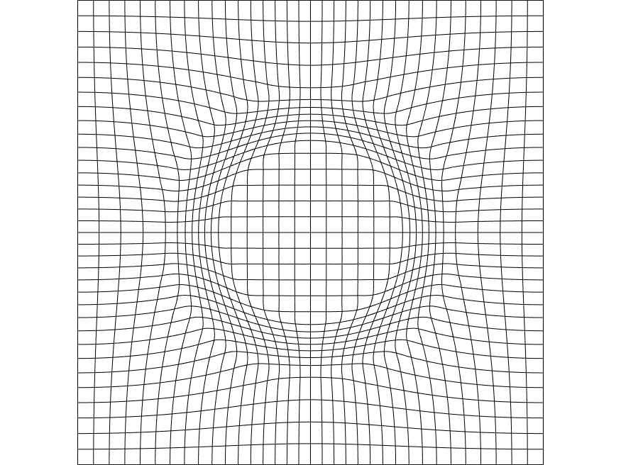
We test the CM method for density redistribution by running the algorithm described in section 3 to time $1$ using Hermite cubic interpolation on various grids of size $N$ and track the decay of $\mathcal{E}$, ${\mathit{h}_{t}}$ is chosen to be $0.1/N$. The results are shown in figure 1, the backward map deforms the domain to concentrate in the selected annulus, the residual energy also exhibits the exponential decay from the diffusion equation.

We briefly describe here the algorithm used to evolve parametric surfaces under a given velocity field in 3D.

Let $\Omega$ be a 3-dimensional domain. For simplicity we assume $\Omega=\mathbb{T}^{3}$ the flat 3-torus. Let ${\bm{v}}:\Omega\times\mathbb{R}_{+}\to\mathbb{R}^{3}$ be a given velocity field. Here we assume that ${\bm{v}}$ is smooth and divergence-free so that the domain transformation it generates is a smooth diffeomorphism of $\Omega$ for all times. We have the same characteristic structure as described in section 2.1 and in [27, 38]. We denote by ${\bm{\Phi}}_{F}$ and ${\bm{\Phi}}_{B}$ the forward and backward characteristic maps, they satisfy the following equations:

The diffeomorphisms are the forward and backward flow-maps of the velocity field ${\bm{v}}$ and have the characteristic structure

for any characteristic curve $\gamma$ satisfying

The forward and backward maps are inverse transformations for all times, i.e.

We denote by ${\bm{\Phi}}_{[t_{1},t_{2}]}$ the forward map in the time interval $[t_{1},t_{2}]$ with ${\bm{\Phi}}_{F}:={\bm{\Phi}}_{[0,t]}$, and we use ${\bm{\Phi}}_{[t_{2},t_{1}]}$ to denote the backward map in the same time-interval, with ${\bm{\Phi}}_{B}:={\bm{\Phi}}_{[t,0]}$. The notation $\mathit{\bm{\Phi}}$ is used for the numerical discretization of the ${\bm{\Phi}}$ maps. The time-stepping can be summarized as

for some grid ${\bm{M}}$ on $\Omega$. The identity $\mathit{\bm{\Phi}}_{[t+{\mathit{h}_{t}},t]}=\mathit{\bm{\Phi}}_{[t,t+{\mathit{h}_{t}}]}^{-1}$ can be guaranteed to high precision by employing higher order ODE integration schemes, and hence the error on the property

stems mainly from the representation quality of the interpolation operator $\mathcal{H}_{\bm{M}}$, which we will control using a dynamic remapping technique described below.

It is well-known that the flow-map possesses a semigroup property which allows for the decomposition of a long-time map into several submaps; this can be used to achieve high resolution representation of the deformation using coarse grid computations. We use the same time-decomposition strategy as in [38] to represent the global-time maps:

The inverse property (36) is controlled numerically by the time-stepping (37). This gives us an alternative a posteriori error estimate for choosing the remapping times $\tau_{i}$. In [38], in the context of the incompressible Euler equations, the remapping time is chosen to the be first time the volume preservation error of the map exceeds some threshold. For surface advection, the velocity is not strictly constrained to divergence free, and volume preservation is not a main concern. Therefore we use the following composition error as remapping criterion.

We then define $\tau_{i}$ to be the first time $t$ where the above error exceeds some chosen threshold.

The forward and backward characteristic maps give us solution operators to the advection problem. Let $S_{0}\subset\Omega$ be an initial curve or surface moving following the velocity field ${\bm{v}}$. Let $S_{t}$ be the surface at time $t$. Using the characteristic maps, we have two equivalent definitions for $S_{t}$, one implicit and the other, explicit:

Equation (41a) uses the same Eulerian definition as in level-set methods. When $S_{0}$ is expressed as the zero-level-set of a function $\psi$, we have that $S_{t}$ is given by the zero-level-set of the advected function $\psi\circ{\bm{\Phi}}_{B}$. This approach is studied in [27], a review of recent advances in level-set methods can be found in [16].

Equation (41b) is a Lagrangian definition, where surfaces are defined explicitly through a parametrization function. This is suitable for curves and surfaces which do not admit a level-set representation, for instance for open curves or non-orientable surfaces. Let $U$ be the parameter space and ${\bm{P}}_{0}:U\to S_{0}\subset\Omega$, a regular parametrization of the surface at time 0, that is, we assume the mapping between $U$ and $S_{0}$ to be a diffeomorphism. The parametrization of $S_{t}$ is then given by

Numerically speaking this method evolves the parametrization function in time using the solution operator $\mathit{\bm{\Phi}}_{F}$. Compared to traditional methods where the surface is sampled and sample points evolved individually, the CM method provides a functional definition of the parametrization function defined everywhere in $U$. Similar to the backward map method in [27], this approach also provides arbitrary resolution of the parametrization function ${\bm{P}}_{t}$, and hence of $S_{t}$. The surface $S_{t}$ can be arbitrarily sampled at any time by evaluating the pushforward operator $\mathit{\bm{\Phi}}_{F}$.

A curve or surface $S_{t}$ can be sampled by choosing sample points ${\bm{y}}_{i}\in U$ and evaluating ${\bm{p}}_{i}(t)={\bm{P}}_{t}({\bm{y}}_{i})$ to represent $S_{t}$ discretely. However, a uniform distribution of ${\bm{y}}_{i}$ in $U$ does not necessarily lead to well-distributed marker points ${\bm{p}}_{i}$ on $S_{t}$. Indeed, as the surface stretches and deforms under the flow, some regions may expand and become sparsely sampled. We can quantify this by evaluating the area-element $A_{t}$ from the first fundamental form $I_{t}=\nabla{\bm{P}}_{t}^{T}\nabla{\bm{P}}_{t}$.

We can compute the time-evolution of $A_{t}$. Using

and applying Jacobi’s rule for derivatives of matrix determinants. We have

Using the cyclic property of the trace operator, we can rewrite this as

where $\Pi_{S_{t}}=\nabla{\bm{P}}_{t}(\nabla{\bm{P}}_{t}^{T}\nabla{\bm{P}}_{t})^{-1}\nabla{\bm{P}}_{t}^{T}$ is the orthogonal projection operator onto the tangent space of $S_{t}$. Therefore, the area-element grows exponentially at rate $\,\text{div}|_{S_{t}}{\bm{v}}$ corresponding to the divergence of the flow along the tangent space of $S_{t}$.

The approach we take to control the growth of the area-element is to modify the parametrization function ${\bm{P}}_{t}$ by applying a transformation on the parametric space $U$. We take $A_{t}$ as a probability density on $U$ and apply the method described in section 2.2 to obtain a mapping ${\bm{X}}_{B}:U\to U$ which pushes the uniform density to the density $A_{t}$. The modified parametrization

should then have area-element $\sqrt{\det I}$ equal to a constant. That is to say, if the points ${\bm{y}}_{i}$ are uniformly distributed in $U$, then the sample points ${\bm{p}}_{i}$ are uniform on $S_{t}$. In practice, it is more efficient to run the surface advection and the area redistribution alongside each other, this means that instead of a fixed initial condition for the diffusion equation of section 2.2, we will use a time-dependent “initial density” given by $A_{t}$. This can be formalized as follows.

We define probability densities on $U$:

We note that both $\rho_{0}$ and $\rho$ are the area-elements corresponding to the parametrizations ${\bm{P}}$ and ${\bm{Q}}$ normalized to a probability density since

We have the following equations for their time evolution:

References

- [1] L. Ambrosio, N. Gigli, and G. Savaré, Gradient flows: in metric spaces and in the space of probability measures, Springer Science & Business Media, 2008.
- [2] D. Appelö and T. Hagstrom, On advection by Hermite methods, Pacific Journal Of Applied Mathematics, 4 (2012), p. 125.
- [3] D. Appelo, T. Hagstrom, and A. Vargas, Hermite methods for the scalar wave equation, SIAM Journal on Scientific Computing, 40 (2018), pp. A3902–A3927.
- [4] L. Balmelli, G. Taubin, and F. Bernardini, Space-optimized texture maps, in Computer Graphics Forum, vol. 21, Eurographics Association, 2002, pp. 411–420.
- [5] J.-D. Benamou and Y. Brenier, A computational fluid mechanics solution to the Monge-Kantorovich mass transfer problem, Numerische Mathematik, 84 (2000), pp. 375–393.
- [6] J.-D. Benamou, Y. Brenier, and K. Guittet, The Monge-Kantorovitch mass transfer and its computational fluid mechanics formulation, International Journal for Numerical methods in fluids, 40 (2002), pp. 21–30.
- [7] J.-D. Benamou, G. Carlier, and M. Laborde, An augmented Lagrangian approach to Wasserstein gradient flows and applications, ESAIM: Proceedings and Surveys, 54 (2016), pp. 1–17.
- [8] M. Bergdorf, G.-H. Cottet, and P. Koumoutsakos, Multilevel adaptive particle methods for convection-diffusion equations, Multiscale Modeling & Simulation, 4 (2005), pp. 328–357.
- [9] M. Bergdorf and P. Koumoutsakos, A Lagrangian particle-wavelet method, Multiscale Modeling & Simulation, 5 (2006), pp. 980–995.
- [10] G. Carlier, V. Duval, G. Peyré, and B. Schmitzer, Convergence of entropic schemes for optimal transport and gradient flows, SIAM Journal on Mathematical Analysis, 49 (2017), pp. 1385–1418.
- [11] J. A. Carrillo, K. Craig, and F. S. Patacchini, A blob method for diffusion, Calculus of Variations and Partial Differential Equations, 58 (2019), pp. 1–53.
- [12] J. A. Carrillo, K. Craig, L. Wang, and C. Wei, Primal dual methods for Wasserstein gradient flows, arXiv preprint arXiv:1901.08081, (2019).
- [13] B. Dacorogna and J. Moser, On a partial differential equation involving the Jacobian determinant, in Annales de l’Institut Henri Poincare (C) Non Linear Analysis, vol. 7, Elsevier, 1990, pp. 1–26.
- [14] P. Gera and D. Salac, Cahn-Hilliard on surfaces: A numerical study, Applied Mathematics Letters, 73 (2017), pp. 56–61.
- [15] P. Gera and D. Salac, Modeling of multicomponent three-dimensional vesicles, Computers & Fluids, 172 (2018), pp. 362–383.
- [16] F. Gibou, R. Fedkiw, and S. Osher, A review of level-set methods and some recent applications, Journal of Computational Physics, 353 (2018), pp. 82–109.
- [17] X. Gu, Y. Wang, T. F. Chan, P. M. Thompson, and S.-T. Yau, Genus zero surface conformal mapping and its application to brain surface mapping, IEEE transactions on medical imaging, 23 (2004), pp. 949–958.
- [18] X. Gu and S.-T. Yau, Global conformal surface parameterization, in Proceedings of the 2003 Eurographics/ACM SIGGRAPH symposium on Geometry processing, Eurographics Association, 2003, pp. 127–137.
- [19] T. Hagstrom and D. Appelö, Solving PDEs with Hermite interpolation, in Spectral and High Order Methods for Partial Differential Equations ICOSAHOM 2014, Springer, 2015, pp. 31–49.
- [20] S. E. Hieber and P. Koumoutsakos, A Lagrangian particle level set method, Journal of Computational Physics, 210 (2005), pp. 342–367.
- [21] W. Huang and R. D. Russell, Adaptive moving mesh methods, vol. 174, Springer Science & Business Media, 2010.
- [22] M. Jin, Y. Wang, S.-T. Yau, and X. Gu, Optimal global conformal surface parameterization, in IEEE Visualization 2004, IEEE, 2004, pp. 267–274.
- [23] R. Jordan, D. Kinderlehrer, and F. Otto, The variational formulation of the Fokker-Planck equation, SIAM journal on mathematical analysis, 29 (1998), pp. 1–17.
- [24] K. Kamrin, C. H. Rycroft, and J.-C. Nave, Reference map technique for finite-strain elasticity and fluid-solid interaction, Journal of the Mechanics and Physics of Solids, 60 (2012), pp. 1952–1969.
- [25] G. Lacombe and S. Mas-Gallic, Presentation and analysis of a diffusion-velocity method, in ESAIM: Proceedings, vol. 7, EDP Sciences, 1999, pp. 225–233.
- [26] R. J. LeVeque, High-resolution conservative algorithms for advection in incompressible flow, SIAM Journal on Numerical Analysis, 33 (1996), pp. 627–665.
- [27] O. Mercier, X.-Y. Yin, and J.-C. Nave, The characteristic mapping method for the linear advection of arbitrary sets, SIAM Journal on Scientific Computing, 42 (2020), pp. A1663–A1685.
- [28] P. Mycek, G. Pinon, G. Germain, and E. Rivoalen, Formulation and analysis of a diffusion-velocity particle model for transport-dispersion equations, Computational and Applied Mathematics, 35 (2016), pp. 447–473.
- [29] J.-C. Nave, R. R. Rosales, and B. Seibold, A gradient-augmented level set method with an optimally local, coherent advection scheme, Journal of Computational Physics, 229 (2010), pp. 3802–3827.
- [30] G. Peyré, Entropic approximation of Wasserstein gradient flows, SIAM Journal on Imaging Sciences, 8 (2015), pp. 2323–2351.
- [31] F. Santambrogio, Optimal transport for applied mathematicians, Birkäuser/Springer, 2015.
- [32] F. Santambrogio, Euclidean, metric, and Wasserstein gradient flows: an overview, Bulletin of Mathematical Sciences, 7 (2017), pp. 87–154.
- [33] B. Seibold, J.-C. Nave, and R. R. Rosales, Jet schemes for advection problems, Discrete and Continuous Dynamical Systems - Series B, 17 (2012), pp. 1229–1259.
- [34] K. Su, L. Cui, K. Qian, N. Lei, J. Zhang, M. Zhang, and X. D. Gu, Area-preserving mesh parameterization for poly-annulus surfaces based on optimal mass transportation, Computer Aided Geometric Design, 46 (2016), pp. 76–91.
- [35] Z. Su, J. Sun, X. Gu, F. Luo, and S.-T. Yau, Optimal mass transport for geometric modeling based on variational principles in convex geometry, Engineering with Computers, 30 (2014), pp. 475–486.
- [36] C. Villani, Optimal transport: old and new, vol. 338, Springer Science & Business Media, 2008.
- [37] A. M. Winslow, Adaptive-mesh zoning by the equipotential method, tech. report, Lawrence Livermore National Lab., CA (USA), 1981.
- [38] X.-Y. Yin, O. Mercier, B. Yadav, K. Schneider, and J.-C. Nave, A characteristic mapping method for the two-dimensional incompressible Euler equations, arXiv preprint arXiv:1910.10841 (Accepted in Journal of Computational Physics), (2020).
- [39] S. Yoshizawa, A. Belyaev, and H.-P. Seidel, A fast and simple stretch-minimizing mesh parameterization, in Proceedings Shape Modeling Applications, 2004., IEEE, 2004, pp. 200–208.
- [40] X. Zhao, Z. Su, X. D. Gu, A. Kaufman, J. Sun, J. Gao, and F. Luo, Area-preservation mapping using optimal mass transport, IEEE Transactions on Visualization and Computer Graphics, 19 (2013), pp. 2838–2847.