跳到论文正文
W Papers独立论文阅读器 arXiv:2008.13035 论文正文 计算阅读时间 · 0%
引用这篇论文根据当前论文元数据生成,正式投稿前建议核对。


License: CC BY 4.0
arXiv:2008.13035v1 [math.SP] 29 Aug 2020

On Ambarzumyan-type Inverse Problems of Vibrating String Equations

Yuri Ashrafyan Thanks: Yuri Ashrafyan: KAUST, CEMSE Division, Thuwal, 23955-6900, KSA, E-mail: yuri.ashrafyan@kaust.edu.sa    Dominik L. Michels Thanks:  Dominik L.˜Michels: KAUST, CEMSE Division, Thuwal, 23955-6900, KSA, E-mail: dominik.michels@kaust.edu.sa
Abstract

We consider the inverse spectral theory of vibrating string equations. In this regard, first eigenvalue Ambarzumyan-type uniqueness theorems are stated and proved subject to separated, self-adjoint boundary conditions. More precisely, it is shown that there is a curve in the boundary parameters’ domain on which no analog of it is possible. Necessary conditions of the nn-th eigenvalue are identified, which allows to state the theorems. In addition, several properties of the first eigenvalue are examined. Lower and upper bounds are identified, and the areas are described in the boundary parameters’ domain on which the sign of the first eigenvalue remains unchanged. This paper contributes to inverse spectral theory as well as to direct spectral theory.

Keywords:  Ambarzumyan theorem, first eigenvalue, inverse problems, vibrating string equations.

MSC 2010:  34A55, 34L15

1 Introduction

When dealing with direct problems, one considers a physical model and calculates a specific output given a specific input. In contrast, inverse problems are dealing with the inversion of this model based on measured or observed outputs, i.e. we consider a mathematical framework which is used to obtain information about parameters of a system from observed measurements. This framework is often useful since it provides information about physical parameters of a system that can usually not directly be observed. As a consequence, inverse problem theory is being developed intensively.

The inverse spectral problems aiming for the reconstruction of operator using spectral data, such as the spectrum (set of eigenvalues), norming constants (L2L^{2}-norms of eigenfunctions), nodal points (roots of eigenfunctions), and other quantities.

Historically, Ambarzumyan did pioneer work [1] with respect to the theory of inverse problems. It is easy to calculate (direct problem) that the eigenvalues of the Sturm-Liouville boundary value problem −y′′=μ​y-y^{\prime\prime}=\mu y, y′​(0)=y′​(π)=0y^{\prime}(0)=y^{\prime}(\pi)=0 are n2,n≥0n^{2},\ n\geq 0. In 1929, Ambarzumyan proved the inverse assertion, if the eigenvalues of the boundary value problem −y′′+q⁡(x)​y=μ​y-y^{\prime\prime}+q(x)y=\mu y, y′​(0)=y′​(π)=0y^{\prime}(0)=y^{\prime}(\pi)=0 are n2,n≥0n^{2},\ n\geq 0, then q⁡(x)=0q(x)=0 a.e. on (0,π)(0,\pi).

Later, Borg [4] showed that with general boundary conditions more information in addition to the spectrum is required in order to uniquely reconstruct the function q⁡(x)q(x). In the same work he showed that two spectra (for different fixed boundary conditions) are sufficient for the unique determination of a problem. Other fundamental work was done by Marchenko [19], who showed that if two problems have the same set of eigenvalues and norming constants, then they coincide. These results were very important and they opened the door for further investigations in inverse spectral theory. Many other kinds of uniqueness theorems for inverse Sturm-Liouville problems have been stated and developed, we just mention several of them here  [17, 13, 21, 8, 7, 9, 28, 2].

Let L⁡(q,γ,δ)L(q,\gamma,\delta) denote the self-adjoint Sturm-Liouville operator generated by the boundary value problem

−y′′+q⁡(s)​y=μ​y,s∈(0,π),μ∈ℂ,\displaystyle-y^{\prime\prime}+q(s)y=\mu y,\qquad s\in(0,\pi),\;\mu\in{\mathbb{C}}, (1.1)
y⁡(0)​cos⁡γ+y′​(0)​sin⁡γ=0,γ∈(0,π],\displaystyle y(0)\cos\gamma+y^{\prime}(0)\sin\gamma=0,\quad\gamma\in(0,\pi], (1.2)
y⁡(π)​cos⁡δ+y′​(π)​sin⁡δ=0,δ∈[0,π),\displaystyle y(\pi)\cos\delta+y^{\prime}(\pi)\sin\delta=0,\quad\delta\in[0,\pi), (1.3)

where the potential function qq is real-valued and summable. It is known, that the spectrum of L⁡(q,γ,δ)L(q,\gamma,\delta) is discrete and consists of real, simple eigenvalues, which we denote by μn=μn​(q,γ,δ)\mu_{n}=\mu_{n}(q,\gamma,\delta), n≥0n\geq 0,

μ0​(q,γ,δ)<μ1​(q,γ,δ)<…<μn​(q,γ,δ)<…,\mu_{0}(q,\gamma,\delta)<\mu_{1}(q,\gamma,\delta)<\ldots<\mu_{n}(q,\gamma,\delta)<\ldots,

emphasizing the dependence of μn\mu_{n} on qq, γ\gamma and δ\delta (see [18, 20, 10]). There are many generalizations of Ambarzumyan’s theorem for the Sturm-Liouville problem in various directions  (see e.g. [7, 15, 5, 7, 31, 6, 29, 30, 3], and the references therein).

Particularly, in [7], it is shown that it is not necessary to specify the whole spectrum: information regarding the first eigenvalue is sufficient. Precisely, if μ0=1π​∫0πq⁡(x)​𝑑x\mu_{0}=\frac{1}{\pi}\int_{0}^{\pi}q(x)dx, then q⁡(x)=μ0q(x)=\mu_{0}, a.e. on (0,π)(0,\pi). This type of problem setting is called a first eigenvalue Ambarzumyan-type inverse problem.

Let AA and A~\tilde{A} be two operators. In what follows, if a certain symbol τ\tau denotes an object related to the operator AA, then τ~\tilde{\tau} will denote a similar object related to A~\tilde{A} and τ^:=τ~−τ\hat{\tau}:=\tilde{\tau}-\tau, τˇ:=τ~/τ\check{\tau}:={\tilde{\tau}}/{\tau}. We recall the inner product (y,z)=∫01y⁡(x)​z⁡(x)¯​𝑑x\left(y,z\right)=\int_{0}^{1}y(x)\overline{z(x)}dx.

In [31], Yurko proved the following generalization of Ambarzumyan theorem for Sturm-Liouville problem (it’s true for any self-adjoint boundary conditions).

Theorem 1.1 (Yurko [31]).

Let q,q~∈Lℝ1​(0,π)q,\,\tilde{q}\in L^{1}_{\mathbb{R}}(0,\pi). If

μ0−μ~0=(q^​φ~0,φ~0)(φ~0,φ~0),\mu_{0}-\tilde{\mu}_{0}=\dfrac{(\hat{q}\tilde{\varphi}_{0},\tilde{\varphi}_{0})}{(\tilde{\varphi}_{0},\tilde{\varphi}_{0})},

where φ~0\tilde{\varphi}_{0} is an eigenfunction of L~\tilde{L} related to μ~0\tilde{\mu}_{0}. Then q⁡(x)=q~​(x)+μ0−μ~0q(x)=\tilde{q}(x)+\mu_{0}-\tilde{\mu}_{0}, a.e. on (0,π)(0,\pi).

Recently, one of the authors [3] has proved another generalization of the first eigenvalue Ambarzumyan-type inverse problem.

Theorem 1.2 ([3]).

Let q,q~∈Lℝ1​(0,π)q,\,\tilde{q}\in L^{1}_{\mathbb{R}}(0,\pi). If

μ0−μ~0=ess​inf⁡q^orμ0−μ~0=ess​sup⁡q^,\mu_{0}-\tilde{\mu}_{0}=\essinf\hat{q}\quad\mbox{or}\quad\mu_{0}-\tilde{\mu}_{0}=\esssup\hat{q},

then q⁡(x)=q~​(x)+μ0−μ~0q(x)=\tilde{q}(x)+\mu_{0}-\tilde{\mu}_{0} a.e. on (0,π)(0,\pi).

The main aim of this paper is to investigate first eigenvalue Ambarzumyan-type theorems for boundary value problems of vibrating string equations:

−u′′=λ​p​(x)​u,x∈(0,1),λ∈ℂ,\displaystyle-u^{\prime\prime}=\lambda p(x)u,\quad x\in(0,1),\quad\lambda\in\mathbb{C}, (1.4)
u⁡(0)​cos⁡α+u′​(0)​sin⁡α=0,α∈(0,π],\displaystyle u(0)\cos\alpha+u^{\prime}(0)\sin\alpha=0,\quad\alpha\in(0,\pi], (1.5)
u⁡(1)​cos⁡β+u′​(1)​sin⁡β=0,β∈[0,π),\displaystyle u(1)\cos\beta+u^{\prime}(1)\sin\beta=0,\quad\beta\in[0,\pi), (1.6)

where the density function pp is piecewise continuous, positive, bounded away from 00, real-valued and λ\lambda is the spectral parameter. This equation describes small transversal vibrations of a string of a linear density pp on the interval [0,1][0,1] (see e.g. [27]). By S⁡(p,α,β)S(p,\alpha,\beta) we denote the self-adjoint operator generated by problem (1.4)–(1.6). It is well-known, that the spectrum of the operator S⁡(p,α,β)S(p,\alpha,\beta) is discrete and consists of real, simple eigenvalues, which we denote by λn=λn​(p,α,β)\lambda_{n}=\lambda_{n}(p,\alpha,\beta), n≥0n\geq 0,

λ0​(p,α,β)<λ1​(p,α,β)<…<λn​(p,α,β)<…,\lambda_{0}(p,\alpha,\beta)<\lambda_{1}(p,\alpha,\beta)<\ldots<\lambda_{n}(p,\alpha,\beta)<\ldots,

emphasizing the dependence of λn\lambda_{n} on pp, α\alpha and β\beta.

The classical Ambarzumyan’s theorem for the operator S⁡(p,π/2,π/2)S(p,\pi/2,\pi/2) on the interval [0,a][0,a] can be stated as follows: if it is known that the eigenvalues are π2​n2/a2\pi^{2}n^{2}/a^{2}, the question is if we can conclude that p⁡(x)=1p(x)=1 on [0,a][0,a]. In [25], Shen constructed a counterexample to this assertion, and showed that one needs additional information about the density function to formulate an inverse problem with one spectrum, such as the function p⁡(x)p(x) being even on [0,a][0,a], or the values of p′​(0)p^{\prime}(0) and p′​(a)p^{\prime}(a) are known. Hence, in general, there is no analog to the Ambarzumyan theorem for string equations in a classical form.

In Section 2, it is shown that first eigenvalue Ambarzumyan-type theorems for the S⁡(p,α,β)S(p,\alpha,\beta) operator are valid, but not for the whole domain α,β∈(0,π]×[0,π)\alpha,\beta\in(0,\pi]\times[0,\pi). It is explained why for some boundary conditions first-eigenvalue inverse problems are impossible. In Section 3, bounds for the lowest eigenvalue are given, and the areas in the boundary parameters’ domain are described, on which it keeps its sign.

2 Main Results

Let φ⁡(x)=φ⁡(x,λ,α,p)\varphi(x)=\varphi(x,\lambda,\alpha,p) be the solution of (1.4), which satisfies the initial conditions

φ⁡(0,λ,α,p)=sin⁡α,φ′​(0,λ,α,p)=−cos⁡α.\varphi(0,\lambda,\alpha,p)=\sin\alpha,\quad\varphi^{\prime}(0,\lambda,\alpha,p)=-\cos\alpha.\\

The eigenvalues λn\lambda_{n} are the solutions of the equation

φ⁡(1,λ,α)​cos⁡β+φ′​(1,λ,α)​sin⁡β=0.\varphi(1,\lambda,\alpha)\cos\beta+\varphi^{\prime}(1,\lambda,\alpha)\sin\beta=0.

It is easy to see that the functions φn​(x):=φ⁡(x,λn,α,p)\varphi_{n}(x):=\varphi(x,\lambda_{n},\alpha,p), n≥0n\geq 0, are the eigenfunctions, corresponding to the eigenvalue λn\lambda_{n}.

Our first eigenvalue Ambarzumyan-type theorems for vibrating string equation are as follows.

Theorem 2.1.

Let α,β∈(0,π]×[0,π)\alpha,\beta\in(0,\pi]\times[0,\pi) and cos⁡α​cos⁡β−sin⁡(α−β)≠0\cos\alpha\cos\beta-\sin(\alpha-\beta)\neq 0, for α,β∈[π/4,π]×[0,3​π/4]\alpha,\beta\in[\pi/4,\pi]\times[0,3\pi/4]. If

λ0=λ~0​maxx∈[0,1]​pˇ​(x)orλ0=λ~0​minx∈[0,1]​pˇ​(x),\lambda_{0}=\tilde{\lambda}_{0}\max_{x\in[0,1]}\check{p}(x)\qquad\mbox{or}\qquad\lambda_{0}=\tilde{\lambda}_{0}\min_{x\in[0,1]}\check{p}(x),

then p⁡(x)=λ~0/λ0​p~​(x)p(x)={\tilde{\lambda}_{0}}/{\lambda_{0}}\tilde{p}(x) on [0,1][0,1].

Proof.

Write down the fact that φ0​(x)\varphi_{0}(x) and φ~0​(x)\tilde{\varphi}_{0}(x) are the eigenfunctions of the operators S⁡(p,α,β)S(p,\alpha,\beta) and S⁡(p~,α,β)S(\tilde{p},\alpha,\beta) corresponding to the eigenvalues λ0\lambda_{0} and λ~0\tilde{\lambda}_{0}, respectively:

−φ0′′​(x)+λ0​p​(x)​φ0​(x)=0,\displaystyle-\varphi_{0}^{\prime\prime}(x)+\lambda_{0}p(x)\varphi_{0}(x)=0, (2.1)
−φ~0′′​(x)+λ~0​p~​(x)​φ~0​(x)=0.\displaystyle-\tilde{\varphi}_{0}^{\prime\prime}(x)+\tilde{\lambda}_{0}\tilde{p}(x)\tilde{\varphi}_{0}(x)=0. (2.2)

Multiplying (2.1) by φ~0​(x)\tilde{\varphi}_{0}(x), (2.2) by φ⁡(x)\varphi(x) and subtracting from the first equation the second one, we obtain

−dd​x​[φ0′​(x)​φ~0​(x)−φ0​(x)​φ~0′​(x)]+\displaystyle-\dfrac{d}{dx}\left[\varphi_{0}^{\prime}(x)\tilde{\varphi}_{0}(x)-\varphi_{0}(x)\tilde{\varphi}_{0}^{\prime}(x)\right]+
+φ0​(x)​φ~0​(x)​[λ0​p​(x)−λ~0​p~​(x)]=0.\displaystyle+\varphi_{0}(x)\tilde{\varphi}_{0}(x)\left[\lambda_{0}p(x)-\tilde{\lambda}_{0}\tilde{p}(x)\right]=0.

Integrating the latter from 00 to 11, we obtain

−φ0′​(1)​φ~0​(1)+φ0​(1)​φ~0′​(1)+\displaystyle-\varphi_{0}^{\prime}(1)\tilde{\varphi}_{0}(1)+\varphi_{0}(1)\tilde{\varphi}_{0}^{\prime}(1)+
+φ0′​(0)​φ~0​(0)−φ0​(0)​φ~0′​(0)+\displaystyle+\varphi_{0}^{\prime}(0)\tilde{\varphi}_{0}(0)-\varphi_{0}(0)\tilde{\varphi}_{0}^{\prime}(0)+
+∫01φ0(x)φ~0(x)[λ0p(x)−λ~0p~(x)]dx=0.\displaystyle+\int_{0}^{1}\varphi_{0}(x)\tilde{\varphi}_{0}(x)\left[\lambda_{0}p(x)-\tilde{\lambda}_{0}\tilde{p}(x)\right]dx=0.

Since φ0​(x)\varphi_{0}(x) and φ~0​(x)\tilde{\varphi}_{0}(x) satisfy the same boundary conditions, thus the first four terms vanish, and we obtain

∫01φ0​(x)​φ~0​(x)​[λ0​p​(x)−λ~0​p~​(x)]​𝑑x=0.\int_{0}^{1}\varphi_{0}(x)\tilde{\varphi}_{0}(x)\left[\lambda_{0}p(x)-\tilde{\lambda}_{0}\tilde{p}(x)\right]dx=0.

In virtue of Sturm’s oscillation theorem (see e.g. [7, 12, 26, 11]), the product φ0​(x)​φ~0​(x)\varphi_{0}(x)\tilde{\varphi}_{0}(x) has no zeros in interval (0,1)(0,1). This with the condition of the theorem complete the proof. ∎

Theorem 2.2.

Let α,β∈(0,π]×[0,π)\alpha,\beta\in(0,\pi]\times[0,\pi) and cos⁡α​cos⁡β−sin⁡(α−β)≠0\cos\alpha\cos\beta-\sin(\alpha-\beta)\neq 0, for α,β∈[π/4,π]×[0,3​π/4]\alpha,\beta\in[\pi/4,\pi]\times[0,3\pi/4]. If

λ0=λ~0​(pˇ​φ~0,φ~0)(φ~0,φ~0)\lambda_{0}=\tilde{\lambda}_{0}\dfrac{\left(\check{p}\tilde{\varphi}_{0},\tilde{\varphi}_{0}\right)}{\left(\tilde{\varphi}_{0},\tilde{\varphi}_{0}\right)}

then p⁡(x)=λ~0/λ0​p~​(x)p(x)={\tilde{\lambda}_{0}}/{\lambda_{0}}\tilde{p}(x) on [0,1][0,1].

Proof.

Taking into account the condition of the theorem, these simple relations are held

(−p−1​φ~0,φ~0)(φ~0,φ~0)=(−p~−1​φ~0,pˇ​φ~0)(φ~0,φ~0)=λ~0​(pˇ​φ~0,φ~0)(φ~0,φ~0)=λ0\dfrac{\left(-p^{-1}\tilde{\varphi}_{0},\tilde{\varphi}_{0}\right)}{\left(\tilde{\varphi}_{0},\tilde{\varphi}_{0}\right)}=\dfrac{\left(-\tilde{p}^{-1}\tilde{\varphi}_{0},\check{p}\tilde{\varphi}_{0}\right)}{\left(\tilde{\varphi}_{0},\tilde{\varphi}_{0}\right)}=\tilde{\lambda}_{0}\dfrac{\left(\check{p}\tilde{\varphi}_{0},\tilde{\varphi}_{0}\right)}{\left(\tilde{\varphi}_{0},\tilde{\varphi}_{0}\right)}=\lambda_{0}

from which follows that φ~0​(x)\tilde{\varphi}_{0}(x) is an eigenfunction of the operator S⁡(p,α,β)S(p,\alpha,\beta) with the eigenvalue λ0\lambda_{0}. Particularly, −φ~0′′​(x)=λ0​p​(x)​φ~0​(x)-\tilde{\varphi}_{0}^{\prime\prime}(x)=\lambda_{0}p(x)\tilde{\varphi}_{0}(x), thus we obtain λ0​p​(x)=λ~0​p~​(x)\lambda_{0}p(x)=\tilde{\lambda}_{0}\tilde{p}(x). This completes the proof. ∎

Remark 1.

Consider the curve cos⁡α​cos⁡β−sin⁡(α−β)=0\cos\alpha\cos\beta-\sin(\alpha-\beta)=0, for α,β∈[π/4,π]×[0,3​π/4]\alpha,\beta\in[\pi/4,\pi]\times[0,3\pi/4], see Figure 1. The first eigenvalue λ0​(p,α,β)\lambda_{0}(p,\alpha,\beta) on this curve is always zero (the proof of this assertion is given in Theorem 3.3). Therefore first-eigenvalue Ambarzumyan-type theorems are impossible for this α\alpha and β\beta.

Figure 1: Illustration of the curve describing λ0​(p,α,β)=0\lambda_{0}(p,\alpha,\beta)=0.
Example 1.

Consider the boundary value problem

−u′′=λ​p​(x)​u,\displaystyle-u^{\prime\prime}=\lambda p(x)u,
u⁡(0)=u⁡(1)=0.\displaystyle u(0)=u(1)=0.

Let p~​(x)=1\tilde{p}(x)=1, then λ~0=π2\tilde{\lambda}_{0}=\pi^{2} and φ~0​(x)=sin⁡π​x\tilde{\varphi}_{0}(x)=\sin\pi x.

Theorem 2.1 implies the following assertion.

Corollary 1.

If

λ0​(p,π,0)=π2​max⁡p−1​(x)\lambda_{0}(p,\pi,0)=\pi^{2}\max p^{-1}(x)

then p⁡(x)=π2/λ0p(x)=\pi^{2}/\lambda_{0} on [0,1][0,1].

Theorem 2.2 implies the following assertion.

Corollary 2.

If

λ0​(p,π,0)=2​π2​∫01p−1​(x)​s​i​n2​(π​x)​𝑑x,\lambda_{0}(p,\pi,0)=2\pi^{2}\int_{0}^{1}p^{-1}(x)sin^{2}(\pi x)dx,

then p⁡(x)=π2/λ0p(x)=\pi^{2}/\lambda_{0} on [0,1][0,1].

As we saw that the lowest eigenvalue contains significant information about the equation, a reasonable question may arise: can one state a uniqueness theorem having information regarding an arbitrary eigenvalue? The answer is positive, but more information is demanded, than in the case of the lowest eigenvalue.

Theorem 2.3.

Let λn≠0\lambda_{n}\neq 0, for a fixed n>0n>0. If

λn=λ~n​(pˇ​φ~n,φ~n)(φ~n,φ~n)andλn=λ~n​maxx∈[0,1]​pˇ​(x),\lambda_{n}=\tilde{\lambda}_{n}\dfrac{\left(\check{p}\tilde{\varphi}_{n},\tilde{\varphi}_{n}\right)}{\left(\tilde{\varphi}_{n},\tilde{\varphi}_{n}\right)}\quad\mbox{and}\quad\lambda_{n}=\tilde{\lambda}_{n}\max_{x\in[0,1]}\check{p}(x),

then p⁡(x)=λ~n/λn​p~​(x)p(x)={\tilde{\lambda}_{n}}/{\lambda_{n}}\tilde{p}(x) on [0,1][0,1].

Proof.

From the first condition we obtain

∫01(λn−λ~n​pˇ​(x))​φ~n2​(x)​𝑑x=0.\int_{0}^{1}(\lambda_{n}-\tilde{\lambda}_{n}\check{p}(x))\tilde{\varphi}_{n}^{2}(x)dx=0.

In virtue of Sturm’s oscillation theorem, it is known that the nn-th eigenfunction has exactly nn isolated zeros in the open interval (0,1)(0,1). Thus, the measure of the set of all zeros is 00. This with the second condition of the theorem yields λn−λ~n​pˇ​(x)=0\lambda_{n}-\tilde{\lambda}_{n}\check{p}(x)=0. This completes the proof. ∎

For Sturm-Liouville problem similar result was proved in [16].

Remark 2.

It is obvious that in Theorem 2.3 the second condition can be replaced with λn=λ~n​minx∈[0,1]​pˇ​(x)\lambda_{n}=\tilde{\lambda}_{n}\min_{x\in[0,1]}\check{p}(x).

3 Exploring the Lowest Eigenvalue

For the case sin⁡γ≠0\sin\gamma\neq 0 and sin⁡δ≠0\sin\delta\neq 0, i.e. γ,δ∈(0,π)\gamma,\delta\in(0,\pi), the boundary conditions (1.2)–(1.3) can be written as

a​y​(0)+y′​(0)=0,\displaystyle a\,y(0)+y^{\prime}(0)=0,
b​y​(π)+y′​(π)=0.\displaystyle b\,y(\pi)+y^{\prime}(\pi)=0.

In [14] the authors showed, that for a Sturm-Liouville problem with fixed boundary conditions (a,b)(a,b) and a q∈L2​(0,π)q\in L^{2}(0,\pi), the lowest eigenvalue has the property

−∞<μ0(q,a,b)≤μ0(e,−(a−b)/2,(a−b)/2),-\infty<\mu_{0}(q,a,b)\leq\mu_{0}\left(e,-(a-b)/2,(a-b)/2\right),

where ee is a known even function (e⁡(x)=e⁡(π−x)e(x)=e(\pi-x)) from L2​(0,π)L^{2}(0,\pi), which is uniquely defined by the eigenvalues μn​(q,a,b),n≥1\mu_{n}(q,a,b),n\geq 1 and the Dirichlet boundary conditions y⁡(0)=y⁡(π)=0y(0)=y(\pi)=0.

In [22], for a q∈L∞​(0,π)q\in L^{\infty}(0,\pi) and the Dirichlet boundary conditions, the following bounds for the lowest eigenvalue is proved:

|μ0​(q,π,0)−μ0​(0,π,0)|≤‖q‖∞.|\mu_{0}(q,\pi,0)-\mu_{0}(0,\pi,0)|\leq\|q\|_{\infty}. (3.1)

In [10], for a qq from Lℝ1​(0,π)L^{1}_{\mathbb{R}}(0,\pi) (in particular Lℝ∞​(0,π)L^{\infty}_{\mathbb{R}}(0,\pi)) and γ∈(0,π]\gamma\in(0,\pi], δ∈[0,π)\delta\in[0,\pi), a formula for μn​(q,γ,δ)\mu_{n}(q,\gamma,\delta) is found, and particularly for n=0n=0:

μ0​(q,γ,δ)=μ0​(0,γ,δ)+∫01∫0πq⁡(x)​h02​(x,t​q,γ,δ)​𝑑x​𝑑t,\mu_{0}(q,\gamma,\delta)=\mu_{0}(0,\gamma,\delta)+\displaystyle\int_{0}^{1}\int_{0}^{\pi}q(x)h^{2}_{0}(x,tq,\gamma,\delta)\,dx\,dt, (3.2)

where h0​(x,t​q,γ,δ)h_{0}(x,tq,\gamma,\delta) is a normalized eigenfunction (∫0πh02​(x,t​q,γ,δ)​𝑑x=1\int_{0}^{\pi}h^{2}_{0}(x,tq,\gamma,\delta)dx=1) of the problem L⁡(t​q,γ,δ)L(tq,\gamma,\delta) and where tt is a real parameter. From (3.2) the generalization of (3.1) follows:

|μ0​(q,γ,δ)−μ0​(0,γ,δ)|≤‖q‖∞,|\mu_{0}(q,\gamma,\delta)-\mu_{0}(0,\gamma,\delta)|\leq\|q\|_{\infty},

which can be written as

−ess​sup⁡|q|≤μ0​(q,γ,δ)−μ0​(0,γ,δ)≤ess​sup⁡|q|.-\esssup|q|\leq\mu_{0}(q,\gamma,\delta)-\mu_{0}(0,\gamma,\delta)\leq\esssup|q|. (3.3)

In the same work it is shown that the lowest eigenvalue tends to −∞-\infty:

limγ→0μ0​(q,γ,δ)=−∞,for fixed​δ∈[0,π),\displaystyle\displaystyle\lim_{\gamma\rightarrow 0}\mu_{0}(q,\gamma,\delta)=-\infty,\qquad\mbox{for fixed}\;\delta\in[0,\pi),
limδ→πμ0​(q,γ,δ)=−∞,for fixed​γ∈(0,π].\displaystyle\displaystyle\lim_{\delta\rightarrow\pi}\mu_{0}(q,\gamma,\delta)=-\infty,\qquad\mbox{for fixed}\;\gamma\in(0,\pi].

We found narrower bounds for the lowest eigenvalue of the Sturm-Liouville operator.

Theorem 3.1.

The lowest eigenvalue of the operator L⁡(q,γ,δ)L(q,\gamma,\delta) has the property

ess​inf⁡q≤μ0​(q,γ,δ)−μ0​(0,γ,δ)≤ess​sup⁡q.\essinf q\leq\mu_{0}(q,\gamma,\delta)-\mu_{0}(0,\gamma,\delta)\leq\esssup q.
Remark 3.

Theorem 3.1 is also true for arbitrary self-adjoint boundary conditions.

Theorem 3.1 is a corollary of Theorem 1.2, when we take q~​(x)≡0\tilde{q}(x)\equiv 0. We can see that our bounds do not contradict the properties mentioned above and are more narrow than in (3.3) because of

−ess​sup⁡|q|≤ess​inf⁡q≤ess​sup⁡q≤ess​sup⁡|q|.-\esssup|q|\,\leq\,\essinf q\,\leq\,\esssup q\,\leq\,\esssup|q|.
Refer to caption
(a) μ0​(0,γ,δ)\mu_{0}(0,\gamma,\delta)
Refer to caption
(b) λ0​(1,α,β)\lambda_{0}(1,\alpha,\beta)
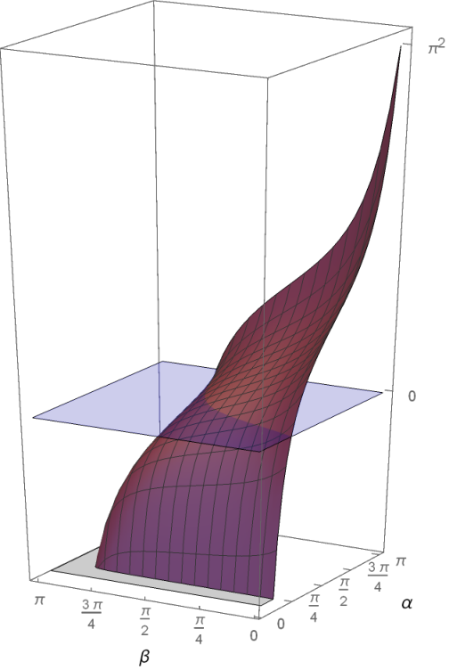
Figure 2: Illustration of the first eigenvalues of L⁡(0,γ,δ)L(0,\gamma,\delta) and S⁡(1,α,β)S(1,\alpha,\beta).

For the first eigenvalue of the vibrating string equation we obtain the following bounds.

Theorem 3.2.

The lowest eigenvalue of operator S⁡(p,α,β)S(p,\alpha,\beta) has the property

λ0​(1,α,β)​minx∈[0,π]​p−1​(x)≤λ0​(p,α,β)≤λ0​(1,α,β)​maxx∈[0,π]​p−1​(x).\lambda_{0}(1,\alpha,\beta)\min_{x\in[0,\pi]}p^{-1}(x)\leq\lambda_{0}(p,\alpha,\beta)\leq\lambda_{0}(1,\alpha,\beta)\max_{x\in[0,\pi]}p^{-1}(x).
Proof.

This is a corollary of Theorem 2.1. ∎

The graphs of eigenvalues μ0​(0,γ,δ)\mu_{0}(0,\gamma,\delta) and λ0​(1,α,β)\lambda_{0}(1,\alpha,\beta) are in Figure 2. The relation between eigenvalues of L⁡(q,γ,δ)L(q,\gamma,\delta) and S⁡(p,α,β)S(p,\alpha,\beta) can be found in the appendix.

Example 2.

Consider the boundary value problem S⁡(xr+1,π,0)S(x^{r}+1,\pi,0), for a fixed r∈ℝ+r\in\mathbb{R}_{+},

−u′′=λ⁡(xr+1)​u,\displaystyle-u^{\prime\prime}=\lambda(x^{r}+1)u,
u⁡(0)=u⁡(1)=0.\displaystyle u(0)=u(1)=0.

Then λ0​(1,π,0)=π2\lambda_{0}(1,\pi,0)=\pi^{2}, and maxx∈[0,π]⁡(xr+1)−1=1\displaystyle\max_{x\in[0,\pi]}(x^{r}+1)^{-1}=1, minx∈[0,π]⁡(xr+1)−1=1/2\displaystyle\min_{x\in[0,\pi]}(x^{r}+1)^{-1}=1/2. Theorem 3.2 implies the following assertion.

Corollary 3.

For any fixed r∈ℝ+r\in\mathbb{R}_{+}:

π2/2≤λ0​(xr+1,π,0)≤π2.\pi^{2}/2\leq\lambda_{0}(x^{r}+1,\pi,0)\leq\pi^{2}.

For instance, when r=1,2, the lowest eigenvalues are λ0​(x+1,π,0)≈6.548\lambda_{0}(x+1,\pi,0)\approx 6.548 and λ0​(x2+1,π,0)≈7.643\lambda_{0}(x^{2}+1,\pi,0)\approx 7.643.

The next theorem shows, that for any density function p⁡(x)p(x) the sign of the first eigenvalue λ0​(p,α,β)\lambda_{0}(p,\alpha,\beta) only depends on the boundary parameters.

Theorem 3.3.

The lowest eigenvalue of the operator S⁡(p,α,β)S(p,\alpha,\beta) has the property

λ0​(p,α,β)​{=0,cos⁡α​cos⁡β−sin⁡(α−β)=0,α,β∈[π/4,π]×[0,3​π/4],>0,cos⁡α​cos⁡β−sin⁡(α−β)<0,α,β∈(π/4,π]×[0,3​π/4),<0,otherwise.\lambda_{0}(p,\alpha,\beta)\left\{\begin{array}[]{lll}=0,&\cos\alpha\cos\beta-\sin(\alpha-\beta)=0,&\alpha,\beta\in[\pi/4,\pi]\times[0,3\pi/4],\\ >0,&\cos\alpha\cos\beta-\sin(\alpha-\beta)<0,&\alpha,\beta\in(\pi/4,\pi]\times[0,3\pi/4),\\ <0,&\mbox{otherwise}.\end{array}\right.
Proof.

First, we will show that the lowest eigenvalue λ0\lambda_{0} is zero for boundary parameters satisfying

cos⁡α​cos⁡β−sin⁡(α−β)=0,α,β∈[π/4,π]×[0,3​π/4].\cos\alpha\cos\beta-\sin(\alpha-\beta)=0,\qquad\alpha,\beta\in[\pi/4,\pi]\times[0,3\pi/4]. (3.4)

Let us check that λ=0\lambda=0 is an eigenvalue. When λ=0\lambda=0 the equation (1.4) becomes

u′′​(x)=0,u^{\prime\prime}(x)=0,

hence, in order for u⁡(x)u(x) to be an eigenfunction of S⁡(p,α,β)S(p,\alpha,\beta) related to an eigenvalue λ=0\lambda=0, it should be linear u⁡(x)=k​x+cu(x)=kx+c, where k2+c2≠0k^{2}+c^{2}\neq 0, and satisfy boundary conditions, (1.5)–(1.6)

u⁡(0)​cos⁡α+u′​(0)​sin⁡α=0,\displaystyle u(0)\cos\alpha+u^{\prime}(0)\sin\alpha=0,
u⁡(1)​cos⁡β+u′​(1)​sin⁡β=0.\displaystyle u(1)\cos\beta+u^{\prime}(1)\sin\beta=0.

For u⁡(x)=k​x+cu(x)=kx+c, we consider the system of linear equations

c​cos⁡α+k​sin⁡α=0,\displaystyle c\cos\alpha+k\sin\alpha=0,\qquad\qquad
c​cos⁡β+k⁡(sin⁡β+cos⁡β)=0.\displaystyle c\cos\beta+k(\sin\beta+\cos\beta)=0.

In order to obtain a unique solution for kk and cc, the determinant should be zero:

|cos⁡αsin⁡αcos⁡βsin⁡β+cos⁡β|=cos⁡α​sin⁡β+cos⁡α​cos⁡β−sin⁡α​cos⁡β\left|\begin{array}[]{cc}\cos\alpha&\sin\alpha\\ \cos\beta&\sin\beta+\cos\beta\end{array}\right|=\cos\alpha\sin\beta+\cos\alpha\cos\beta-\sin\alpha\cos\beta

which is zero by the condition. Therefore, λ=0\lambda=0 is an eigenvalue, and it remains to show that this is the smallest eigenvalue. Let there be a number n0>0n_{0}>0 such that λn0=0\lambda_{n_{0}}=0. This means that there exists σ≠0\sigma\neq 0, such that the smallest eigenvalue λ0=−σ2\lambda_{0}=-\sigma^{2}. Thus, the equation (1.4) can be rewritten as

u0′′​(x)=σ2​p​(x)​u0​(x).u^{\prime\prime}_{0}(x)=\sigma^{2}p(x)u_{0}(x). (3.5)

Now we separate the curve into following three cases:

  1. 1.

    α∈[π/4,π/2),β∈[0,π/2)\alpha\in[\pi/4,\pi/2),\beta\in[0,\pi/2),

  2. 2.

    α=β=π/2\alpha=\beta=\pi/2,

  3. 3.

    α∈(π/2,π],β∈(π/2,3​π/4]\alpha\in(\pi/2,\pi],\beta\in(\pi/2,3\pi/4].

We will only show the proof for the first case since the other two cases are completely similar. In this case the boundary conditions become

u0​(0)+u0′​(0)​(tan⁡β+1)=0,\displaystyle u_{0}(0)+u^{\prime}_{0}(0)(\tan\beta+1)=0,
u0​(1)+u0′​(1)​tan⁡β=0.\displaystyle u_{0}(1)+u^{\prime}_{0}(1)\tan\beta=0.

Subtracting from the second condition the first one, we obtain

(u0′​(1)−u0′​(0))​tan⁡β+(u0​(1)−u0​(0)−u0′​(0))=0.(u^{\prime}_{0}(1)-u^{\prime}_{0}(0))\tan\beta+(u_{0}(1)-u_{0}(0)-u^{\prime}_{0}(0))=0.

For simplicity, it can be written as

a​tan⁡β+b=0.a\tan\beta+b=0.

To find aa and bb, we integrate (3.5) from 00 to 0<t≤10<t\leq 1 and afterwards, from 00 to 11:

u0′​(t)−u0′​(0)=σ2​∫0tp⁡(x)​u0​(x)​𝑑x,\displaystyle u^{\prime}_{0}(t)-u^{\prime}_{0}(0)=\sigma^{2}\int_{0}^{t}p(x)u_{0}(x)dx,
u0′​(1)−u0′​(0)=σ2​∫01p⁡(x)​u0​(x)​𝑑x=a,\displaystyle u^{\prime}_{0}(1)-u^{\prime}_{0}(0)=\sigma^{2}\int_{0}^{1}p(x)u_{0}(x)dx=a,
u0​(1)−u0​(0)−u′​(0)=σ2​∫01∫0tp⁡(x)​u0​(x)​𝑑x​𝑑t=b.\displaystyle u_{0}(1)-u_{0}(0)-u^{\prime}(0)=\sigma^{2}\int_{0}^{1}\int_{0}^{t}p(x)u_{0}(x)dxdt=b.

Since the density function p⁡(x)p(x) is positive and u0​(x)u_{0}(x) has no zeros, due to the oscillation theorem, in the whole interval (0,1)(0,1), therefore a≠0a\neq 0, b≠0b\neq 0 and they have the same sign. Now, please note that tan⁡β≥0\tan\beta\geq 0, for β∈[0,π/2)\beta\in[0,\pi/2), so the relation a​tan⁡β+b=0a\tan\beta+b=0 is impossible. Thus, the first eigenvalue cannot be negative and λ0=0\lambda_{0}=0.

Here we proof the second assertion of the theorem, that is λ0​(p,α,β)>0\lambda_{0}(p,\alpha,\beta)>0, when α,β∈[π/4,π]×[0,3​π/4]\alpha,\beta\in[\pi/4,\pi]\times[0,3\pi/4] and

cos⁡α​cos⁡β−sin⁡(α−β)<0.\cos\alpha\cos\beta-\sin(\alpha-\beta)<0. (3.6)

The third one of the theorem can be handled in a similar way. Please note, that we can show this for λ0​(1,α,β)\lambda_{0}(1,\alpha,\beta), after it, in virtue of Theorem 3.2, it will be spread on λ0​(p,α,β)\lambda_{0}(p,\alpha,\beta).

Assume that λ0​(1,α,β)<0\lambda_{0}(1,\alpha,\beta)<0, i.e. there exists σ≠0\sigma\neq 0, such that λ0=−σ2\lambda_{0}=-\sigma^{2}. So, the boundary value problem (1.4)–1.6 for p⁡(x)=1p(x)=1 is being written as

u0′′​(x)=σ2​u0​(x),\displaystyle u^{\prime\prime}_{0}(x)=\sigma^{2}u_{0}(x),
u0​(0)​cos⁡α+u0′​(0)​sin⁡α=0,\displaystyle u_{0}(0)\cos\alpha+u^{\prime}_{0}(0)\sin\alpha=0,
u0​(1)​cos⁡β+u0′​(1)​sin⁡β=0.\displaystyle u_{0}(1)\cos\beta+u^{\prime}_{0}(1)\sin\beta=0.

The solution of this problem has the following form:

u⁡(x)=A​e|σ|​x+B​e−|σ|​x,u(x)=Ae^{|\sigma|x}+Be^{-|\sigma|x},

where A2+B2≠0A^{2}+B^{2}\neq 0. Inserting this into the boundary conditions, we obtain

A⁡(cos⁡α+|σ|​sin⁡α)+B⁡(cos⁡α−|σ|​sin⁡α)=0,\displaystyle A(\cos\alpha+|\sigma|\sin\alpha)+B(\cos\alpha-|\sigma|\sin\alpha)=0,\qquad\qquad
A​e|σ|​(cos⁡β+|σ|​sin⁡β)+B​e−|σ|​(cos⁡β−|σ|​sin⁡β)=0.\displaystyle Ae^{|\sigma|}(\cos\beta+|\sigma|\sin\beta)+Be^{-|\sigma|}(\cos\beta-|\sigma|\sin\beta)=0.

To have a unique solution for AA and BB, the determinant should be zero:

D:=|cos⁡α+|σ|​sin⁡αcos⁡α−|σ|​sin⁡αe|σ|​(cos⁡β+|σ|​sin⁡β)e−|σ|​(cos⁡β−|σ|​sin⁡β)|=\displaystyle D:=\left|\begin{array}[]{cc}\cos\alpha+|\sigma|\sin\alpha&\cos\alpha-|\sigma|\sin\alpha\\ e^{|\sigma|}(\cos\beta+|\sigma|\sin\beta)&e^{-|\sigma|}(\cos\beta-|\sigma|\sin\beta)\end{array}\right|=
=cos⁡α​cos⁡β⁡(e−|σ|−e|σ|)+sin⁡(α−β)​|σ|​(e−|σ|+e|σ|)+sin⁡α​sin⁡β​σ2​(e|σ|−e−|σ|)=\displaystyle=\cos\alpha\cos\beta(e^{-|\sigma|}-e^{|\sigma|})+\sin(\alpha-\beta)|\sigma|(e^{-|\sigma|}+e^{|\sigma|})+\sin\alpha\sin\beta\sigma^{2}(e^{|\sigma|}-e^{-|\sigma|})=
=2(−cosαcosβsinh|σ|+sin(α−β)|σ|cosh|σ|+sinαsinβσ2sinh|σ|).\displaystyle=2(-\cos\alpha\cos\beta\sinh|\sigma|+\sin(\alpha-\beta)|\sigma|\cosh|\sigma|+\sin\alpha\sin\beta\sigma^{2}\sinh|\sigma|).

Taking into account (3.6), for DD we obtain

D>2(cosαcosβ(|σ|cosh|σ|−sinh|σ|)+sinαsinβσ2sinh|σ|),D>2(\cos\alpha\cos\beta(|\sigma|\cosh|\sigma|-\sinh|\sigma|)+\sin\alpha\sin\beta\sigma^{2}\sinh|\sigma|),

or

D>2(sin(α−β)(|σ|cosh|σ|−sinh|σ|)+sinαsinβσ2sinh|σ|).D>2(\sin(\alpha-\beta)(|\sigma|\cosh|\sigma|-\sinh|\sigma|)+\sin\alpha\sin\beta\sigma^{2}\sinh|\sigma|).

Please note that sinαsinβσ2sinh|σ|≥0\sin\alpha\sin\beta\sigma^{2}\sinh|\sigma|\geq 0, for all α,β∈(π/4,π]×[0,3​π/4)\alpha,\beta\in(\pi/4,\pi]\times[0,3\pi/4). Let us show that |σ|​cosh|σ|−sinh⁡|σ|>0|\sigma|\cosh|\sigma|-\sinh|\sigma|>0. Consider

f⁡(x):=x​cosh⁡x−sinh⁡xf(x):=x\cosh x-\sinh x (3.7)

for x>0x>0. Differentiating (3.7), we obtain

f′​(x)=x​sinh⁡x.f^{\prime}(x)=x\sinh x.

Since f⁡(0)=0f(0)=0 and f′​(x)>0f^{\prime}(x)>0, for all x>0x>0, thus f⁡(x)>0f(x)>0.

Now we separate the domain into the following three subdomains:

  1. 1.

    α∈(π/4,π/2],β∈[0,π/2)\alpha\in(\pi/4,\pi/2],\beta\in[0,\pi/2),

  2. 2.

    α∈(π/2,π],β∈[0,π/2)\alpha\in(\pi/2,\pi],\beta\in[0,\pi/2),

  3. 3.

    α∈(π/2,π],β∈[π/2,3​π/4)\alpha\in(\pi/2,\pi],\beta\in[\pi/2,3\pi/4).

For the first and the third case cos⁡α​cos⁡β≥0\cos\alpha\cos\beta\geq 0, and for the second case sin⁡(α−β)≥0\sin(\alpha-\beta)\geq 0. Thus D>0D>0 and we come to contradiction. This completes the proof. ∎

Remark 4.

Since on the curve cos⁡α​cos⁡β−sin⁡(α−β)=0\cos\alpha\cos\beta-\sin(\alpha-\beta)=0, for α,β∈[π/4,π]×[0,3​π/4]\alpha,\beta\in[\pi/4,\pi]\times[0,3\pi/4], the first eigenvalue is always zero, thus the inequality in Theorem 3.2 holds also for this case.

4 Conclusion

This paper deals with the inverse spectral theory of vibrating string equations subject to separated, self-adjoint boundary conditions. It is shown, that in spite of the fact that there is no classical Ambarzumyan’s theorem analog for string equations, the first eigenvalue Ambarzumyan-type theorems are valid for some domain in the boundary conditions (Theorems 2.1–2.2 and the extension for the nn-th eigenvalue in Theorem 2.3).

The curve in the boundary conditions’ domain (α,β∈(0,π]×[0,π)\alpha,\beta\in(0,\pi]\times[0,\pi)), on which no analog of the first eigenvalue theorem is possible, is given by the equation cos⁡α​cos⁡β−sin⁡(α−β)=0\cos\alpha\cos\beta-\sin(\alpha-\beta)=0, for α,β∈[π/4,π]×[0,3​π/4]\alpha,\beta\in[\pi/4,\pi]\times[0,3\pi/4] (see Figure 1). The explanation simply follows from one property of the first eigenvalue, as on that curve it is always zero, despite of the density function p⁡(x)p(x). This property is given in Theorem 3.3 together with another property, which states that the sign of the first eigenvalue is always positive (negative) on the right (left) area from that curve in the boundary parameters’ domain.

It is well known that the set of eigenvalues is bounded from below. In Theorem 3.2, the exact lower and upper bounds are found for the lowest eigenvalue depending on boundary parameters and the density function.

Acknowledgements

This work has been supported by KAUST (individual baseline funding).

References

  • [1] V. Ambarzumian. Über eine Frage der Eigenwerttheorie. Zeitschrift für Physik, 53:690–695.
  • [2] Yu.A. Ashrafyan. A new kind of uniqueness theorems for inverse Sturm–Liouville problems. Boundary Value Problems, 2017(79), 2017.
  • [3] Yu.A. Ashrafyan. A remark on Ambarzumian’s theorem. Results in Mathematics, 73:36(1), 2018.
  • [4] G. Borg. Eine Umkehrung der Sturm–Liouvilleschen Eigenwertaufgabe. Acta Math., 78:1–96, 1946.
  • [5] N.K. Chakravarty and S.K. Acharyya. On an extension of the theorem of V.A. Ambarzumyan. Proc. Roy. Soc. Edinb. A, 110:79–84, 1988.
  • [6] H.H. Chern, C.K. Law, and H.J. Wang. Extension of ambarzumyan’s theorem to general boundary conditions. J. Math. Anal. Appl, 263:333–342, 2001. (Corrigendum – J. Math. Anal. Appl, 309:764–768, 2005).
  • [7] G. Freiling and V.A. Yurko. Inverse Sturm–Liouville problems and their applications. Nova Science Publishers, Inc., New York, 2001.
  • [8] F. Gesztesy and B. Simon. Inverse spectral analysis with partial information on the potential, II. the case of discrete spectrum. Trans. Amer. Math. Soc., 352:2765–2787, 2000.
  • [9] T.N. Harutunyan. On a uniqueness theorem in the inverse sturm-liouville problem. Mat. Vestnik, 61:139–147, 2009.
  • [10] T.N. Harutyunyan. The dependence of the eigenvalues of the sturm-liouville problem on boundary conditions. Mat. Vestnik, 60(4):285–294, 2008.
  • [11] T.N. Harutyunyan, A.A. Pahlevanyan, and Yu.A. Ashrafyan. On the “movement” of the zeros of eigenfunctions of the sturm-liouville problem. Proceedings of Artsakh State University, 1(27):12–20, 2013. (Russian) (English version: http://arxiv.org/abs/1608.04246).
  • [12] D. Hinton. Sturm’s 1836 oscillation results. evolution of the theory. Sturm-Liouville Theory: Past and Present (Birkhäuser Verlag), pages 1–27, 2005.
  • [13] H. Hochstadt and B. Lieberman. An inverse sturm-liouville problem with mixed given data. SIAM J. Appl. Math., 34:676–680, 1978.
  • [14] E.L. Isaacson, H.P. McKean, and E. Trubowitz. The inverse sturm-liouville problem, II. Com. Pure and Appl. Math., 37:1–11, 1984.
  • [15] N.V. Kuznezov. Extensions of V.A. Ambarzumyan theorem. Dokl. Akad. Nauk, 146:1259–1262, 1962.
  • [16] A.A. Kıraç. An extension of the first eigen-type ambarzumyan theorem. Methods of Functional Analysis and Topology, 26(2):167–168, 2020.
  • [17] N. Levinson. The inverse Sturm–Liouville problem. Mat. Tidsskr., B., pages 25–30, 1949.
  • [18] B.M. Levitan and I.S. Sargsyan. Sturm-Liouville and Dirac operators. Nauka, Moskva, 1988. (in Russian).
  • [19] V.A. Marchenko. Concerning the theory of a differential operator of the second order. Doklady Akad. Nauk., SSSR, 72:457–460, 1950. (in Russian).
  • [20] V.A. Marchenko. Sturm–Liouville operators and its applications. Naukova Dumka, Kiiv, 1977. (in Russian).
  • [21] J. McLaughlin and W. Rundell. A uniqueness theorem for an inverse sturm-liouville problem. 28(7):1471–1472, 1987.
  • [22] J. Poschel and E. Trubowitz. Inverse spectral theory. New-York, Academic Press, 1987.
  • [23] C.-L. Shen. The liouville transformation, the density function, and the complete transformability problem of the potential equation. Inverse Problems, 21(2):615–634, 2005.
  • [24] C.-L. Shen. On the liouville transformation and some inverse spectral problems. Inverse Problems, 21(2):591–614, 2005.
  • [25] C.-L. Shen. On some inverse spectral problems related to the ambarzumyan problem and the dual string of the string equation. Inverse Problems, 23:2417–2436, 2007.
  • [26] B. Simon. Sturm oscillation and comparison theorems. Sturm-Liouville Theory: Past and Present (Birkhäuser Verlag), pages 29–43, 2005.
  • [27] G. Wei and H.-K. Xu. Inverse spectral problem for a string equation with partial information. Inverse Problems, 26:115004(14pp), 2010.
  • [28] Z. Wei and G. Wei. Uniqueness results for inverseSturm-Liouville problems with partial information given on the potential and spectral data. Boundary Value Problems, 200:1–16, 2016.
  • [29] C.F. Yang, Z.Y. Huang, and X.P. Yang. Ambarzumyan’s theorems for vectorıal Sturm-Liouville systems with coupled boundary conditions. Taiwanese Journal Of Mathematics, 14(4):1429–1437, 2010.
  • [30] E. Yilmaz and H. Koyunbakan. Ambarzumyan type theorem for a matrix valued quadratic Sturm-Liouville problem. Computer Modeling in Engineering and Sciences, 99(6):463–471, 2014.
  • [31] V.A. Yurko. On ambarzumyan-type theorems. Applied Mathematics Letters, 26:506–509, 2013.

Appendix: Relation of S⁡(p,α,β)S(p,\alpha,\beta) and L⁡(q,γ,δ)L(q,\gamma,\delta)

Let the density function be p∈C2​[0,1]p\in C^{2}[0,1]. Then we can use the Liouville transformation (see e.g. [24, 23]):

s⁡(x)=πc​∫0xp⁡(t)​𝑑t,y⁡(s)=π2c2​p1/4​(x)​u​(x),\displaystyle s(x)=\dfrac{\pi}{c}\int_{0}^{x}\sqrt{p(t)}dt,\,\,\,y(s)=\dfrac{\pi^{2}}{c^{2}}p^{1/4}(x)u(x),
q(s)=p−1/4(x)d2d​s2(p1/4(x)),\displaystyle q(s)=p^{-1/4}(x)\frac{d^{2}}{ds^{2}}(p^{1/4}(x)),

where c=∫01p⁡(t)​𝑑tc=\int_{0}^{1}\sqrt{p(t)}dt, to transform S⁡(p,α,β)S(p,\alpha,\beta) into L⁡(q,γ,δ)L(q,\gamma,\delta). Please note that s⁡(0)=0s(0)=0 and s⁡(1)=πs(1)=\pi, therefore s∈[0,π]s\in[0,\pi]. For boundary parameters we obtain

{cot⁡α=cπ​(cot⁡γp1/2​(0)+p′​(0)4​p3/2​(0)),if​γ∈(0,π),α=π,if​γ=π,\left\{\begin{array}[]{cc}\cot\alpha=\dfrac{c}{\pi}\left(\dfrac{\cot\gamma}{p^{1/2}(0)}+\dfrac{p^{\prime}(0)}{4p^{3/2}(0)}\right),&\textrm{if}\;\gamma\in(0,\pi),\\ \alpha=\pi,&\mbox{if}\;\gamma=\pi,\end{array}\right.
{β=0,if​δ=0,cot⁡β=cπ​(cot⁡δp1/2​(1)+p′​(1)4​p3/2​(1)),if​δ∈(0,π),\left\{\begin{array}[]{cc}\beta=0,&\textrm{if}\;\delta=0,\\ \cot\beta=\dfrac{c}{\pi}\left(\dfrac{\cot{\delta}}{p^{1/2}(1)}+\dfrac{p^{\prime}(1)}{4p^{3/2}(1)}\right),&\textrm{if}\;\delta\in(0,\pi),\end{array}\right.

and for the eigenvalues

λn​(p,α,β)=π2c2​μn​(q,γ,δ).\lambda_{n}(p,\alpha,\beta)=\dfrac{\pi^{2}}{c^{2}}\mu_{n}(q,\gamma,\delta).

When we take p⁡(x)≡1p(x)\equiv 1, then c=1c=1 and q⁡(x)≡0q(x)\equiv 0, thus λn​(1,α,β)=π2​μn​(0,γ,δ)\lambda_{n}(1,\alpha,\beta)=\pi^{2}\mu_{n}(0,\gamma,\delta). The latter relation is demonstrated in Figure 2.