∎

Adaptive Exploitation of Pre-trained Deep Convolutional Neural Networks for Robust Visual Tracking

Seyed Mojtaba Marvasti-Zadeh Hossein Ghanei-Yakhdan Shohreh Kasaei

Received: date / Accepted: date

Abstract

Due to the automatic feature extraction procedure via multi-layer nonlinear transformations, the deep learning-based visual trackers have recently achieved a great success in challenging scenarios for visual tracking purposes. Although many of those trackers utilize the feature maps from pre-trained convolutional neural networks (CNNs), the effects of selecting different models and exploiting various combinations of their feature maps are still not compared completely. To the best of our knowledge, all those methods use a fixed number of convolutional feature maps without considering the scene attributes (e.g., occlusion, deformation, and fast motion) that might occur during tracking. As a pre-requisition, this paper proposes adaptive discriminative correlation filters (DCF) based on the methods that can exploit CNN models with different topologies. First, the paper provides a comprehensive analysis of four commonly used CNN models to determine the best feature maps of each model. Second, with the aid of analysis results as attribute dictionaries, an adaptive exploitation of deep features is proposed to improve the accuracy and robustness of visual trackers regarding video characteristics. Third, the generalization of proposed method is validated on various tracking datasets as well as CNN models with similar architectures. Finally, extensive experimental results demonstrate the effectiveness of proposed adaptive method compared with the state-of-the-art visual tracking methods.

Keywords:

Discriminative correlation filters deep convolutional neural networks robust visual tracking

1 Introduction

Generic visual tracking is a fundamental task in computer vision, which aims to estimate the motion trajectory of an unknown target over time Marvasti-Zadeh et al. 2019a; Li et al. 2018c. It is included in various practical applications such as automated surveillance and navigation systems, autonomous robots, and self-driving cars Brunetti et al. 2018; Marvasti-Zadeh et al. 2020; Chang et al. 2019. In recent years, discriminative correlation filters (DCF) based trackers (e.g., Danelljan et al. 2017b; Danelljan et al. 2017a; Galoogahi et al. 2017; Marvasti-Zadeh et al. 2019b) have achieved great attention considering their robustness to the photometric/geometric variations and significant computational efficiency. The primary purpose of these trackers is to increase the discriminative power of correlation filters to distinguish a target from its background. However, their performance can be dramatically affected by practical scene attributes such severe occlusion, background clutter, deformation, viewpoint change, low resolution, fast camera motion, and heavy illumination variation.
It is undeniable that feature extraction is a critical component of visual trackers to meaningfully represent an visual object or a part of it. Besides, the effective selection of features, considering scene information, plays a crucial role in the performance of the DCF-based trackers. Although some visual tracking methods typically use hand-crafted features (e.g., histogram of oriented gradients (HOG), histogram of local intensities (HOI), global color histogram (GCH), and Color-Names (CN)), deep features have been successfully employed for visual tracking purposes Marvasti-Zadeh et al. 2019a; Li et al. 2018c. To provide unique features of a target and strength the robustness, recent visual tracking methods (e.g., Tang et al. 2019b; Yi et al. 2019; Li et al. 2019a; Li et al. 2018a; Danelljan et al. 2017a; Li et al. 2018d) generally exploit fixed number of feature maps extracted from CNNs. However, these trackers have not considered that adaptive utilization of high-dimensional deep features may result in higher learning accuracy (by removing redundant or noisy features), lower computational cost, and better model interpretation. By doing so, deep features can simultaneously provide descriptiveness and flexibility against challenging attributes.
Roughly speaking, deep learning-based visual trackers can be categorized into the feature extraction networks (FENs) and end-to-end networks (EENs) Li et al. 2018c. The FENs are referred to the trackers that employ deep features extracted by pre-trained CNN models into the traditional frameworks such as DCFs. In contrast, the EENs directly evaluate target candidates by the fine-tuned/trained networks on visual tracking datasets. This work will be focused on the exploitation of FENs in the DCF framework. Although most of the recent DCF-based trackers have used deep features, they still utilize various CNN models and different layers of each model. For instance, these trackers widely employ AlexNet Krizhevsky et al. 2012 (e.g., Held et al. 2016; Sun et al. 2018; Zhai et al. 2016) and VGG-Net Chatfield et al. 2014; Simonyan and Zisserman 2014 models, while deeper CNN models are not exhaustively investigated yet. Table 1 lists the most popular CNN models, which have been pre-trained on the ImageNet dataset Russakovsky et al. 2015. Coming to this end, the motivations of this work is to figure out about: 1) the best CNN model as well as the best feature maps of four models for visual tracking purposes, 2) the best combinations of deep features, 3) the robustness of feature maps related to scene attributes, and 4) the adaptive exploitation of best feature maps. Fig. 1 shows a brief overview of this work for DCF-based visual trackers, which employ FENs for feature extraction.

Figure 1: A brief overview of this work for adaptive exploitation of deep features in DCF framework.

The main contributions are as follows. First, as a pre-requisition to exploit various CNN models with different topologies, a modified efficient convolution operators tracker is proposed. Second, a comprehensive analysis of four popular pre-trained CNN models (namely, VGG-M Chatfield et al. 2014, VGG-16 Simonyan and Zisserman 2014, GoogLeNet Szegedy et al. 2015, and ResNet-50 He et al. 2016, which have perceptible differences in terms of error rates) is provided. It ranks the best exploitations of features maps for visual tracking purposes. By the achieved results of the comprehensive analysis, attribute dictionaries are proposed for each model to exploit the best feature maps related to different situations of challenging scenarios. Hence, the first to the third aforementioned motivations are answered by a comprehensive analysis, appropriately. Then, based on the attribute dictionaries of each model, an adaptive exploitation method of deep features is proposed for answering to the fourth motivation. Furthermore, generalization of the proposed method into other DCF-based visual trackers is validated by the aid of the proposed deep background-aware correlation filters (DeepBACF) method. Moreover, the generalization of attribute dictionaries is extensively investigated on the pre-trained ResNeXt-50 Xie et al. 2017, SE-ResNet-50 Hu et al. 2018, and SE-ResNeXt-50 Hu et al. 2018 models, which have similar architectures as the ResNet-50 model. Finally, the performance of the best proposed adaptive method is extensively evaluated with the state-of-the-art trackers on well-known visual tracking datasets. To the best of our knowledge, this is the first work that comprehensively evaluates CNN models and their feature maps for visual tracking purposes. Moreover, this is the first proposed method that investigate adaptive exploitation of different convolutional layers depending on possible challenging attributes of video sequences for visual tracking.
The rest of the paper is organized as follows. The overview of related work is described in Section 2. In Section 3, the four CNN models are comprehensively analyzed, and then the proposed adaptive method for using the best CNN feature maps is presented. Extensive experimental results on visual tracking datasets are given in Section 4. Finally, the conclusion and future work are summarized in Section 5.

Table 1: Most popular CNN models, number of layers, and corresponding error rates for the classification task.

CNN Model	Year	Number of Layers	Top-1 Error	Top-5 Error
AlexNet Krizhevsky et al. 2012	2012	8	41.8	19.2
VGG-M Chatfield et al. 2014	2013	8	37.1	15.8
VGG-16 (config. D) Simonyan and Zisserman 2014	2014	16	28.5	9.9
VGG-19 Simonyan and Zisserman 2014	2014	19	28.7	9.9
GoogLeNet Szegedy et al. 2015	2014	22	34.2	12.9
ResNet-50 He et al. 2016	2015	50	24.6	7.7

2 Related Work

In this section, the diverse exploitation of CNN models and corresponding layers in recent visual trackers are highlighted. In fact, this brief review of the related work reveals the necessity of comprehensive analysis (Sec. 3.1) to use these CNN models in visual tracking. Related works are classified according to various CNN models. Moreover, the details of the employment of models, layers, and datasets are listed in Table 2.
VGG-M Model: Spatially regularized discriminative correlation filters tracker (DeepSRDCF) Danelljan et al. 2016a aims to learn more discriminative appearance models on larger search regions. By introducing spatial regularization weights, its formulation penalizes unwanted boundary effects of standard DCF-based methods. To learn a target model in the continuous spatial domain, continuous convolution operator tracker (C-COT) Danelljan et al. 2016b employs multi-resolution deep feature maps and an implicit interpolation model for accurate sub-pixel localization of target. Also, efficient convolution operators tracker (ECO) Danelljan et al. 2017a tackles the computational complexity and over-fitting problem of the C-COT by factorized convolutions, a compact model of training sample distribution, and conservative update strategy. Based on ECO, two trackers weighted ECO (WECO) He et al. 2018 and VDSR-SRT Lin and Yuan 2018 have been proposed. While the WECO tracker introduces a weighted sum operation and feature normalization, the VDSR-SRT tracker addresses the tracking in low-resolution images by a super-resolution algorithm. To exploit temporal information, spatial-temporal regularized correlation filters tracker (STRCF) Li et al. 2018a utilizes a temporal regularization term as well as a spatial one to iteratively optimize its filters by the alternating direction method of multipliers algorithm (ADMM) Boyd et al. 2010. Also, weighted aggregation with enhancement filter tracker (WAEF) Rout et al. 2019 employs temporal Tikhonov regularization to provide better features and suppress unrelated frames. Region of interest (ROI) pooled correlation filters tracker (RPCF) Sun et al. 2019 aims to compress model size by utilizing smaller feature maps. Finally, target-aware correlation filters tracker (TACF) Li et al. 2019a learns guided filters to prevent from background and distractors.

Table 2: Exploited FENS in some visual tracking methods.

Visual Tracking Method	Model	Pre-training Dataset	Name of Exploited Layer(s)
DeepSRDCF Danelljan et al. 2016a	VGG-M	ImageNet	Conv1
C-COT Danelljan et al. 2016b	VGG-M	ImageNet	Conv1, Conv5
ECO Danelljan et al. 2017a	VGG-M	ImageNet	Conv1, Conv5
WECO He et al. 2018	VGG-M	ImageNet	Conv1, Conv5
VDSR-SRT Lin and Yuan 2018	VGG-M	ImageNet	Conv1, Conv5
DeepSTRCF Li et al. 2018a	VGG-M	ImageNet	Conv3
WAEF Rout et al. 2019	VGG-M	ImageNet	Conv1, Conv5
RPCF Sun et al. 2019	VGG-M	ImageNet	Conv1, Conv5
DeepTACF Li et al. 2019a	VGG-M	ImageNet	Conv1
ETDL Yi et al. 2019	VGG-16	ImageNet	Conv1-2
FCNT Wang et al. 2015	VGG-16	ImageNet	Conv4-3, Conv5-3
DNT Chi et al. 2017	VGG-16	ImageNet	Conv4-3, Conv5-3
CREST Song et al. 2017	VGG-16	ImageNet	Conv4-3
CPT Che et al. 2019	VGG-16	ImageNet	Conv5-1, Conv5-3
DeepFWDCF Du et al. 2018	VGG-16	ImageNet	Conv4-3
DTO Wang et al. 2018b	VGG-16, SSD	ImageNet	Conv3-3, Conv4-3, Conv5-3
HCFT Ma et al. 2015	VGG-19	ImageNet	Conv3-4, Conv4-4, Conv5-4
HCFTs Ma et al. 2018a	VGG-19	ImageNet	Conv3-4, Conv4-4, Conv5-4
LCTdeep Ma et al. 2018b	VGG-19	ImageNet	Conv5-4
HDT Qi et al. 2016	VGG-19	ImageNet	Conv4-2, Conv4-3, Conv4-4, Conv5-2, Conv5-3, Conv5-4
IBCCF Li et al. 2018b	VGG-19	ImageNet	Conv3-4, Conv4-4, Conv5-4
DCPF Mozhdehi and Medeiros 2017	VGG-19	ImageNet	Conv3-4, Conv4-4, Conv5-4
MCPF Zhang et al. 2017	VGG-19	ImageNet	Conv3-4, Conv4-4, Conv5-4
MCCT Wang et al. 2018a	VGG-19	ImageNet	Conv4-4, Conv5-4
ORHF Liu et al. 2018	VGG-19	ImageNet	Conv3-4, Conv4-4, Conv5-4
IMM-DFT Tang et al. 2019b	VGG-19	ImageNet	Conv3-4, Conv4-4, Conv5-4
DeepHPFT Li et al. 2018d	VGG-16, VGG-19, and GoogLeNet	ImageNet	Conv5-3, Conv5-4, and icp6-out

VGG-16 Models: Enhanced tracking and detection learning method (ET -DL) Yi et al. 2019 consists of adaptive multi-scale DCFs and a re-detection module to robustly track a target and find it after failures. To separate category detection and distraction determination, deep fully convolutional networks tracker (FCNT) Wang et al. 2015 uses distinct convolutional layers and a feature map selection method. Thereby, the computational burden can be reduced, and irrelevant features can be discarded. Dual network-based tracker (DNT) Chi et al. 2017 embeds boundary and shape information into deep features to enjoy more effective features for visual tracking. Also, CREST tracker Song et al. 2017 integrates the processes of learning DCFs with feature extraction to provide more appropriate features for visual tracking. Moreover, adaptive feature weighted DCF tracker (FWDCF) Du et al. 2018 weights deep features by a segmentation model to suppress the background and distractors. To adaptively leverage low-dimensional features, channel pruning tracker (CPT) Che et al. 2019 provides a channel pruned VGG-16 model, average feature energy ratio method, and adaptive iterative strategy for target localization. In contrast to mentioned trackers, deep tracking with objectness method Wang et al. 2018b assumes that the tracker is aware of object categories to investigate its effect on tracking performance.
VGG-19 Models: Hierarchical correlation feature-based tracker (HCFT) Ma et al. 2015 learns multi-level correlation response maps on multiple convolutional layers to simultaneously alleviate appearance variation and precisely localize the target. Also, the modified HCFT (called HCFTs or HCFT*) Ma et al. 2018a partially compares the performance of three CNN models (i.e., AlexNet, VGG-19, and ResNet-152) and adds two region proposals and a classifier to HCFT for long-term visual tracking purposes. However, insufficient exploration of ResNet’s feature maps results in imperfect visual tracking. Deep long-term correlation tracker (LCTdeep) Ma et al. 2018b consists of distinctive DCFs, pyramidal features, short-term & and long-term learning rates, and an incrementally learned detector to improve the tracking robustness in presence of significant appearance change and scale variation. By using an online decision-theoretical Hedge algorithm, hedged deep tracker (HDT) Qi et al. 2016 aggregates weak CNN-based trackers for exploring advantages of hierarchical feature maps. To handle aspect ratio variation, 1D Boundary and 2D Center CFs tracker (IBCCF) provides a family of boundary CFs and optimizes the boundary and center correlation filters. By exploiting particle filters, the DCPF Mozhdehi and Medeiros 2017 tracker strengthens deep features to discriminate the target from its background. Multi-task correlation particle filter tracker (MCPF) considers inter-dependencies among deep features to cover multiple modes in the posterior density of the target state. Besides, DeepHPFT tracker Li et al. 2018d exploits hand-crafted and deep features in particle filter framework to improve the visual tracking performance. To decide based on reliable localization, MCCT tracker Wang et al. 2018a constructs various DCFs that employ different features to learn different target models. To preserve computational complexity, ORHF tracker Liu et al. 2018 validates the estimated confidence scores and selects effective deep features. Lastly, IMM-DFT tracker Tang et al. 2019b considers insufficiency of linear combination of deep features and provides adaptive hierarchical features for visual tracking.
In contrast to existing FEN-based visual trackers, this work reviews all possible exploration of four widely used CNN models for visual tracking. By doing a comprehensive analysis, two attribute dictionaries for the CNN models are provided. These dictionaries do not follow concrete rules to employ into visual trackers. Thus, the dictionaries are considered as the keys to effectively select the most appropriate features regarding video characteristics or an estimation of them. To validate the analysis results, the generalization of the dictionaries are assessed on different visual tracking datasets, CNN models with similar architectures, and another DCF-based tracker. Owing to the analyses and dictionaries, effective adaptive exploitation of deep features will be possible. Therefore, an adaptive method is proposed, which can simply integrate into the DCF-based trackers to improve discrimination ability of target modeling.

3 Proposed Visual Tracking Method

In this section, the architecture of the four most popular CNN models and the reason for choosing them in the comprehensive analysis is briefly mentioned. Then, the comprehensive analysis and main results of the CNN models are presented. By this analysis, the best features of each model related to the challenging attributes are provided. Finally, a method for adaptive exploitation of these models is proposed.

3.1 Comprehensive Analysis of Pre-trained CNN Models

As shown in Table 1, the most popular CNN models have just a slight difference in performance (e.g., the VGG-16 and VGG-19). As such, in this work, the model with lower complexity is selected. Also, the AlexNet has considerably less performance than others. Thus, four commonly used CNN models, namely VGG-M, VGG-16, GoogLeNet, and ResNet-50 are selected (for more details, see Chatfield et al. 2014; Simonyan and Zisserman 2014; Szegedy et al. 2015; He et al. 2016). Table 3 shows the the configuration of models and test layers (denoted by D1 to D5) in this work. Regarding the topologies of these models, the architectures include either a simple multi-layer stack of non-linear layers (i.e., VGG-M and VGG-Net) or a directed acyclic graph topology (i.e., GoogLeNet and ResNet), which allows designing more complex designs with multiple inputs/outputs for layers. As a pre-requisition to compare the models, this paper proposes a modified ECO tracker which can exploit different CNN models using advanced deep learning modules (i.e., modifying the feature extraction process of ECO tracker by employing AutoNN, and McnExtraLayers modules in MatConvNet toolbox Vedaldi and Lenc 2015). The ECO tracker Danelljan et al. 2017a fuses CNN and hand-crafted features, while it reduces the dimension of deep features by the principal component analysis (PCA) and a down-sampling strategy. However, in order to have fair and meaningful comparisons, the modified ECO tracker (Sec. 3.1.1) and the proposed adaptive method (Sec. 3.2) do not fuse CNN features with hand-crafted ones and also do not apply down-sampling or dimensional reduction processes.

Table 3: Configuration of pre-trained CNN models. [Convolutional layers are denoted as “Conv

<

filter size

>

<

filter depth

>

”.]

VGG-Medium (8-layers)		VGG-Net (16-layers, configuration D)		GoogLeNet (22-layers)		ResNet-50 (50-layers)
Test Output	Layers	Test Output	Layers	Test Output	Layers	Test Output	Layers
D1	Conv7-96	Conv3-64		D1	Conv7-64	D1	Conv7-64
		D1	Conv3-64
LRN		max pool		max pool		max pool
max pool		Conv3-128		D2	Conv3-192
		D2	Conv3-128			Conv1-64		$\times 3$
D2	Conv5-256	max pool		max pool		Conv3-64
				Inception (3a)		D2	Conv1-256
max pool		Conv3-256		D3	Inception (3b)	Conv1-128		$\times 4$
		Conv3-256		max pool		Conv3-128
Conv3-512		D3	Conv3-256			D3	Conv1-512
Conv3-512		max pool
D3	Conv3-512	Conv3-512		Inception (4a)		Conv1-256		$\times 6$
		Conv3-512		Inception (4b)		Conv3-256
max pool		D4	Conv3-512	Inception (4c)		D4	Conv1-1024
				Inception (4d)
		max pool				Conv1-512		$\times 3$
FC-4096				D4	Inception (4e)	Conv3-512
		Conv3-512		max pool		D5	Conv1-2048
		Conv3-512		Inception (5a)
FC-4096				D5	Inception (5b)	average pool
		D5	Conv3-512	average pool
		max pool
FC-1000		FC-4096		Dropout (40%)		FC-1000
		FC-4096		FC-1000
Soft-max		FC-1000		Soft-max		Soft-max
		Soft-max

The comprehensive analyses of convolutional layers for each model are listed in Table 4 and Table 5. To improve the evaluation speeds, all subsequent layers after the last test layers (i.e., the D3 or D5 output) are removed. In contrast to other works, all of the single layers and also all possible combinations of layers of the models are investigated in this paper. Also, the best (First to third) and the worst feature maps for visual tracking purposes are ranked in these tables. Furthermore, the challenging attributes are categorized based on the factors related to object, camera, and environment. This categorization facilitates exploring these results for the proposed adaptive method (Sec. 3.2).
In this paper, all evaluations are based on the well-known precision and success metrics. The overlap success metric is the percentage of frames that their overlap score of estimated and ground-truth bounding boxes is more than a specific threshold while the distance precision metric is defined as the percentage of frames that their estimated location error with the ground-truth location is smaller than a particular threshold. Note that the default thresholds of standard benchmarks (i.e., 50% overlap and 20 pixels) are used for the evaluations Wu et al. 2015. The success and precision results of the comprehensive analyses of the CNN models on the OTB-2013 dataset Wu et al. 2013, their resolution, and the number of feature maps are listed in Table 4 and Table 5. These tables present the results on more than 29000 frames for each evaluated case of CNN models. In this work, visual tracking datasets Wu et al. 2013; Wu et al. 2015; Liang et al. 2015 have common challenging attributes including illumination variation (IV), out-of-plane rotation (OPR), scale variation (SV), occlusion (OCC), deformation (DEF), motion blur (MB), fast motion (FM), in-plane rotation (IPR), out-of-view (OV), background clutter (BC), and low resolution (LR). Note that due to extensive evaluations, only the best and worst CNN layers are presented (see Appendix A for more details). These tables provide an excellent perspective to use these CNN models and their features for visual tracking. Besides, the pros and cons of the models, layers, and combinations regarding each attribute are clarified. These analyses encourage other visual trackers to propose more sophisticated adaptive methods but also employ precise CNN layers for improving their performance in the presence of specific destructive attributes.

Table 4: Success analysis results for pre-trained CNN models on OTB-2013 dataset. [The first to third best layers and the worst layer in each case are shown with green, blue, yellow, and red color, respectively. The multi-resolution feature maps are abbreviated by “MR”.]

Model	Layers	Features: Resolution/Depth	Overall	Attributes
				Object				Camera				Environment
				SV	DEF	OPR	IPR	FM	MB	LR	OV	BC	OCC	IV
VGG-M	D1	109x109 / 96	0.797	0.727	0.831	0.759	0.713	0.741	0.754	0.598	0.840	0.719	0.807	0.752
	D2	26x26 / 256	0.827	0.752	0.891	0.798	0.727	0.787	0.799	0.659	0.901	0.752	0.856	0.752
	D3	13x13 / 512	0.661	0.645	0.643	0.644	0.610	0.639	0.687	0.383	0.599	0.620	0.700	0.591
	D1, D2	MR / 352	0.802	0.737	0.879	0.774	0.697	0.797	0.824	0.694	0.858	0.728	0.844	0.763
	D1, D3	MR / 608	0.813	0.756	0.841	0.780	0.732	0.801	0.829	0.701	0.931	0.749	0.840	0.783
	D2, D3	MR / 768	0.816	0.766	0.826	0.784	0.718	0.799	0.807	0.672	0.913	0.746	0.831	0.742
	D1, D2, D3	MR / 864	0.823	0.751	0.866	0.793	0.729	0.787	0.806	0.660	0.905	0.736	0.871	0.738
VGG-16	D4	28x28 / 512	0.849	0.792	0.893	0.836	0.778	0.822	0.818	0.671	0.924	0.775	0.889	0.772
	D5	14x14 / 512	0.649	0.637	0.609	0.639	0.619	0.653	0.635	0.398	0.609	0.542	0.647	0.668
	D1, D2	MR / 192	0.754	0.679	0.789	0.705	0.647	0.685	0.680	0.560	0.743	0.652	0.779	0.663
	D2, D5	MR / 640	0.741	0.700	0.747	0.691	0.612	0.688	0.685	0.591	0.734	0.678	0.756	0.677
	D3, D4	MR / 768	0.801	0.730	0.854	0.764	0.723	0.739	0.795	0.710	0.775	0.744	0.818	0.715
	D3, D5	MR / 768	0.791	0.739	0.824	0.755	0.689	0.760	0.769	0.673	0.824	0.716	0.830	0.731
	D4, D5	MR / 1024	0.833	0.793	0.846	0.816	0.779	0.822	0.807	0.644	0.913	0.731	0.869	0.739
	D1, D4, D5	MR / 1078	0.825	0.766	0.845	0.796	0.733	0.805	0.797	0.704	0.894	0.752	0.886	0.762
	D2, D3, D4	MR / 896	0.798	0.747	0.836	0.760	0.706	0.772	0.778	0.713	0.886	0.707	0.830	0.730
	D3, D4, D5	MR / 1280	0.821	0.755	0.856	0.790	0.735	0.770	0.770	0.713	0.875	0.743	0.856	0.747
	D2, D3, D4, D5	MR / 1408	0.804	0.759	0.803	0.756	0.686	0.790	0.791	0.711	0.878	0.741	0.830	0.763
	D1, D2, D3, D4, D5	MR / 1472	0.792	0.757	0.795	0.752	0.689	0.788	0.788	0.714	0.871	0.735	0.821	0.757
GoogLeNet	D3	28x28 / 256	0.818	0.767	0.879	0.786	0.711	0.762	0.756	0.526	0.778	0.715	0.843	0.732
	D4	14x14 / 528	0.774	0.730	0.875	0.779	0.704	0.732	0.691	0.519	0.799	0.785	0.831	0.726
	D5	7x7 / 832	0.395	0.333	0.332	0.395	0.419	0.398	0.362	0.299	0.354	0.404	0.373	0.422
	D2, D3	MR / 448	0.822	0.764	0.865	0.792	0.726	0.785	0.811	0.705	0.889	0.761	0.856	0.752
	D2, D4	MR / 720	0.811	0.745	0.864	0.778	0.710	0.764	0.785	0.702	0.881	0.748	0.839	0.737
	D3, D4	MR / 784	0.822	0.765	0.875	0.792	0.746	0.744	0.791	0.701	0.774	0.762	0.855	0.716
	D3, D5	MR / 1088	0.820	0.770	0.876	0.789	0.718	0.761	0.737	0.539	0.790	0.712	0.845	0.730
	D4, D5	MR / 1360	0.791	0.759	0.877	0.791	0.760	0.759	0.713	0.621	0.758	0.858	0.809	0.781
	D1, D2, D3	MR / 512	0.819	0.760	0.866	0.788	0.720	0.784	0.804	0.693	0.874	0.761	0.854	0.754
	D1, D2, D4	MR / 784	0.801	0.747	0.860	0.764	0.694	0.752	0.773	0.705	0.873	0.723	0.837	0.737
	D1, D3, D4	MR / 848	0.774	0.750	0.768	0.730	0.660	0.763	0.778	0.707	0.840	0.725	0.809	0.716
	D2, D3, D4	MR / 976	0.798	0.754	0.816	0.761	0.686	0.769	0.785	0.711	0.885	0.753	0.812	0.742
	D2, D3, D5	MR / 1280	0.827	0.771	0.870	0.798	0.731	0.784	0.807	0.693	0.878	0.764	0.869	0.753
	D3, D4, D5	MR / 1616	0.840	0.793	0.876	0.815	0.752	0.789	0.798	0.676	0.870	0.766	0.881	0.745
ResNet-50	D1	112x112 / 64	0.789	0.741	0.799	0.759	0.719	0.704	0.707	0.597	0.707	0.691	0.787	0.725
	D3	28x28 / 512	0.825	0.760	0.874	0.796	0.726	0.807	0.823	0.696	0.918	0.775	0.871	0.766
	D4	14x14 / 1024	0.734	0.709	0.767	0.736	0.681	0.732	0.696	0.389	0.711	0.700	0.761	0.605
	D5	7x7 / 2048	0.478	0.453	0.380	0.502	0.500	0.423	0.451	0.178	0.356	0.322	0.465	0.432
	D1, D3	MR / 576	0.811	0.765	0.858	0.778	0.712	0.765	0.783	0.676	0.816	0.727	0.856	0.746
	D3, D4	MR / 1536	0.811	0.766	0.833	0.777	0.706	0.818	0.822	0.691	0.904	0.764	0.839	0.766
	D3, D5	MR / 2560	0.829	0.766	0.883	0.801	0.735	0.816	0.830	0.704	0.930	0.762	0.871	0.763
	D1, D3, D4	MR / 1600	0.815	0.762	0.864	0.783	0.717	0.777	0.771	0.688	0.848	0.723	0.864	0.751
	D1, D3, D5	MR / 2624	0.814	0.756	0.862	0.782	0.716	0.781	0.789	0.708	0.858	0.733	0.864	0.754
	D3, D4, D5	MR / 3584	0.815	0.769	0.837	0.782	0.710	0.829	0.843	0.708	0.940	0.772	0.847	0.777
	D1, D3, D4, D5	MR / 3648	0.810	0.754	0.850	0.777	0.719	0.780	0.777	0.714	0.860	0.707	0.856	0.742

Table 5: Precision analysis results for pre-trained CNN models on OTB-2013 dataset. [The first to third best layers and the worst layer in each case are shown with green, blue, yellow, and red color, respectively. The multi-resolution feature maps are abbreviated by “MR”.]

Model	Layers	Features: Resolution/Depth	Overall	Attributes
				Object				Camera				Environment
				SV	DEF	OPR	IPR	FM	MB	LR	OV	BC	OCC	IV
VGG-M	D1	109x109 / 96	0.895	0.860	0.903	0.891	0.846	0.804	0.808	0.594	0.848	0.815	0.898	0.837
	D2	26x26 / 256	0.884	0.841	0.916	0.874	0.814	0.816	0.783	0.673	0.894	0.785	0.913	0.812
	D3	13x13 / 512	0.752	0.738	0.724	0.764	0.734	0.677	0.731	0.377	0.561	0.697	0.762	0.705
	D1, D2	MR / 352	0.897	0.874	0.919	0.901	0.837	0.855	0.847	0.702	0.860	0.827	0.939	0.845
	D1, D3	MR / 608	0.906	0.884	0.905	0.905	0.862	0.855	0.855	0.711	0.927	0.850	0.928	0.872
	D2, D3	MR / 768	0.870	0.848	0.871	0.856	0.789	0.823	0.792	0.669	0.897	0.788	0.884	0.813
	D1, D2, D3	MR / 864	0.873	0.818	0.872	0.861	0.797	0.814	0.788	0.670	0.896	0.793	0.924	0.778
VGG-16	D3	56x56 / 256	0.886	0.861	0.886	0.879	0.819	0.817	0.788	0.676	0.842	0.824	0.915	0.822
	D4	28x28 / 512	0.905	0.877	0.921	0.905	0.853	0.861	0.855	0.729	0.934	0.833	0.944	0.850
	D5	14x14 / 512	0.746	0.752	0.701	0.750	0.715	0.710	0.691	0.453	0.593	0.608	0.731	0.665
	D1, D2	MR. / 192	0.835	0.772	0.826	0.813	0.747	0.761	0.685	0.559	0.750	0.754	0.863	0.727
	D1, D4	MR / 576	0.894	0.862	0.904	0.887	0.851	0.808	0.829	0.723	0.772	0.839	0.927	0.816
	D3, D4	MR / 768	0.885	0.849	0.906	0.879	0.841	0.796	0.815	0.732	0.783	0.824	0.917	0.808
	D4, D5	MR / 1024	0.898	0.879	0.898	0.895	0.855	0.855	0.839	0.704	0.921	0.808	0.932	0.829
	D1, D3, D4	MR / 832	0.891	0.859	0.905	0.886	0828	0.812	0.780	0.720	0.882	0.806	0.925	0.819
	D1, D4, D5	MR / 1078	0.889	0.853	0.861	0.881	0.822	0.853	0.838	0.725	0.899	0.835	0.954	0.809
	D2, D3, D4	MR / 896	0.893	0.862	0.904	0.888	0.831	0.813	0.781	0.731	0.888	0.808	0.928	0.820
	D2, D3, D4, D5	MR / 1408	0.884	0.882	0.851	0.877	0.817	0.846	0.830	0.726	0.877	0.837	0.913	0.843
	D1, D2, D3, D4, D5	MR / 1472	0.886	0.886	0.851	0.878	0.819	0.849	0.832	0.728	0.879	0.841	0.915	0.844
GoogLeNet	D2	56x56 / 192	0.890	0.861	0.901	0.885	0.827	0.838	0.824	0.702	0.876	0.829	0.927	0.836
	D3	28x28 / 256	0.870	0.857	0.903	0.858	0.793	0.803	0.768	0.521	0.755	0.759	0.888	0.805
	D5	7x7 / 832	0.556	0.474	0.539	0.559	0.553	0.445	0.443	0.367	0.383	0.539	0.511	0.565
	D2, D3	MR / 448	0.904	0.886	0.901	0.903	0.850	0.847	0.830	0.715	0.885	0.837	0.947	0.842
	D2, D4	MR / 720	0.891	0.860	0.901	0.885	0.828	0.805	0.773	0.717	0.879	0.803	0.923	0.814
	D2, D5	MR / 1024	0.870	0.823	0.859	0.859	0.794	0.800	0.769	0.700	0.876	0.798	0.920	0.779
	D3, D4	MR / 784	0.879	0.841	0.904	0.868	0.827	0.769	0.781	0.719	0.774	0.805	0.898	0.783
	D3, D5	MR / 1088	0.861	0.840	0.903	0.845	0.777	0.768	0.717	0.538	0.770	0.731	0.868	0.781
	D4, D5	MR / 1360	0.866	0.859	0.895	0.887	0.879	0.841	0.807	0.787	0.791	0.914	0.846	0.855
	D1, D2, D3	MR / 512	0.903	0.884	0.898	0.901	0.847	0.841	0.821	0.706	0.870	0.837	0.944	0.838
	D1, D3, D4	MR / 848	0.848	0.830	0.786	0.826	0.755	0.831	0.808	0.719	0.848	0.841	0.884	0.789
	D2, D3, D4	MR / 976	0.872	0.861	0.848	0.861	0.797	0.808	0.773	0.728	0.885	0.807	0.891	0.816
	D2, D3, D5	MR / 1280	0.902	0.882	0.900	0.900	0.846	0.845	0.827	0.706	0.876	0.836	0.946	0.841
	D3, D4, D5	MR / 1616	0.906	0.888	0.907	0.902	0.849	0.849	0.834	0.699	0.876	0.833	0.945	0.835
	D1, D3, D4, D5	MR / 1680	0.843	0.820	0.787	0.820	0.747	0.813	0.789	0.725	0.854	0.825	0.874	0.776
ResNet-50	D3	28x28 / 512	0.900	0.869	0.913	0.896	0.839	0.863	0.847	0.716	0.925	0.835	0.943	0.851
	D5	7x7 / 2048	0.606	0.621	0.565	0.623	0.593	0.408	0.447	0.217	0.307	0.466	0.586	0.551
	D3, D4	MR / 1536	0.885	0.876	0.867	0.876	0.813	0.874	0.852	0.700	0.921	0.836	0.914	0.851
	D3, D5	MR / 2560	0.901	0.870	0.918	0.897	0.840	0.866	0.852	0.719	0.933	0.829	0.941	0.846
	D1, D3, D4	MR / 1600	0.884	0.848	0.903	0.874	0.814	0.815	0.781	0.720	0.879	0.811	0.913	0.816
	D1, D3, D5	MR / 2624	0.886	0.851	0.899	0.877	0.819	0.827	0.834	0.734	0.887	0.819	0.918	0.823
	D2, D3, D5	MR / 2816	0.865	0.862	0.832	0.850	0.787	0.827	0.804	0.708	0.849	0.835	0.881	0.821
	D3, D4, D5	MR / 3584	0.893	0.889	0.870	0.887	0.827	0.879	0.866	0.731	0.951	0.836	0.929	0.854
	D1, D3, D4, D5	MR / 3648	0.878	0.837	0.888	0.866	0.813	0.812	0.782	0.732	0.885	0.794	0.901	0.803

3.1.1 Comprehensive Analysis Results

In the following, the fundamental remarks of comprehensive analysis are presented.
Remark 1: It is evident from the results that the last convolutional layer of CNN models has the worst tracking performance. The reason is that these models have been trained to classify objects in the last layer. Due to strategies of dimension reduction (e.g., pooling layers), the last convolutional layers have a low spatial resolution such that the accurate localization of the target is not possible. This observation has already been demonstrated by Danelljan et al. 2016b; Wang et al. 2015; Ma et al. 2015; Ma et al. 2018a as the last convolutional layer captures the semantic object category while suffering from a coarse resolution for accurate localization.
Remark 2: Most of deep learning-based trackers Wang et al. 2015; Gladh et al. 2016; Chi et al. 2017; Ma et al. 2018a; Li et al. 2018c; Marvasti-Zadeh et al. 2019a have mentioned that the multi-level feature maps (shallow & deep convolutional layers) enhances the performance of visual trackers. For example, these multi-level features mostly improve scale estimation process of visual trackers. However, there is not any specific rule on how to combine the CNN feature maps to achieve the best visual tracking performance. For example, deep visual trackers in Wang et al. 2015; Chi et al. 2017 utilize the combination of D4 and D5 layers from the VGG-16 model. This combination provides 1024 feature maps and leads to the second rank in performance evaluation while the single D4 layer from this model has 512 feature maps and achieves the best performance regarding the success and precision metrics. Depending on the desired precision, success, and computational complexity (more feature maps, more complexity), Table 4 and Table 5 indicate the most reasonable features and combinations for visual tracking.
Remark 3: The increase in the number of feature maps does not always improve the tracking performance but also considerably increases the computational complexity. However, it may enhance the performance in the presence of specific attributes. For instance, the combination of D3, D4, and D5 of ResNet-50 improves the tracking performance against the SV, FM, MB, OV, and IV attributes. Note that it generally adds redundant feature maps that are not properly involving to discriminate the target from its background. Hence, blindly increase the number of feature maps may significantly reduce both the tracking speed and the performance. For example, this observation has been employed in FCNT tracker Wang et al. 2015 such that a feature map selection process is performed on the D4 and D5 layers of the VGG-16 model to avoid over-fitting on noisy feature maps.
Remark 4: The most destructive impact on performance is related to the LR. This problem is originated from the limited number of pixels that represent target information. Recently, this issues has been investigated in various computer vision tasks Tong et al. 2020; Yang et al. 2019; Marvasti-Zadeh et al. 2020. According to the achieved results, employing shallow and deep convolutional layers could alleviate this deficiency.
Remark 5: Although the use of a fixed number of layers brings simplicity, adaptive exploitation of deep features grants flexibility to visual tracking methods. Considering analysis results, deep features provide distinct responses to the attributes. Thereby, fixed features possibly reduce the tracking performance in challenging scenarios and also limits the robustness of trackers. Therefore, visual trackers can select different CNN layers based on their application or aims to enhance the accuracy, robustness, or a trade-off between accuracy and robustness. Moreover, the feature maps do not equally respond to the attributes (each layer might be sensitive to some of them) due to different parameters and architectures of CNN models. For instance, the D4 layer in the VGG-16 model has the most acceptable results against the most attributes while low-resolution targets dramatically impact on its performance. Moreover, the efficiency level for each layer is related to the objective of each visual tracker. As such, based on the precision, success, or both, the layer(s) selection options may differ. This important property was in fact the primary motivation of this paper to adaptively exploit the CNN feature maps for visual tracking.
To integrate all the benefits into an adaptive visual tracking method, the following proposed adaptive method exploits the results of the comprehensive analysis (i.e., Table 4 and Table 5) as the attribute dictionaries of the CNN models, referred as precision and success dictionaries. These attribute dictionaries include apparent and latent characteristics of models, which are effective for visual tracking.

3.2 Proposed Adaptive Exploitation of Deep Features

The proposed method composed of determination of an attribute vector, integration of attribute dictionaries into the DCF formulations, and a DCF-based tracker. Furthermore, the proposed method can be more sophistically incorporated into other DCF-based tracking methods considering their specific characteristics.

3.2.1 Attribute Vector Determination

Visual attributes can be roughly categorized according to the related characteristics of object, camera, and environment. As a result, visual trackers can use such categorized attributes to create an attribute vector for their applications. Some of these attributes can be effortlessly specified from the initial bounding box of a target in the first frame. For instance, an object recognition process can specify whether the object is rigid or non-rigid; Or, target resolution can be determined by counting its number of pixels. Moreover, visual tracking methods can achieve valuable information about visual attributes based on specific applications; as an example, different options that can be adjusted by a user. Visual attribute detection methods Liu et al. 2017; Shreyamsha Kumar et al. 2019; Gu et al. 2019; Tang et al. 2019a also can be incorporated with visual trackers for estimating an attribute vector for each frame. Moreover, the visual tracking methods can estimate visual attributes based on their definitions in visual tracking datasets; For instance, the definition of IV, SV, BC, MB, DEF, object motion, camera motion, aspect-ratio change, scene complexity, and absolute motion in Kristan et al. 2015. However, this section focuses on the investigation of adaptive exploitation of deep features and its effects on tracking performance. Thus, employing approaches for visual attribute detection are beyond the objectives of this section and will be studied in future works. But, the per-frame estimation of attribute vectors is still an open problem in visual tracking.
It is assumed that an attribute vector (i.e., a full or incomplete vector) is provided for the visual tracker hereafter. For each application, the attribute vector will be an eleven-component vector such that each component is specified by zero or one (binary values). If there is a probability of occurring each attribute, the corresponding component will be set to one. Hence, the proposed method can adaptively select the best features according to the specified attribute vector, which can represent all the joint combinations of challenging attributes. It is evident that the proposed method selects the best overall feature layers if all components of the attribute vector are zero or one. In this work, the attribute vector of each video sequence is exploited which is provided by visual tracking datasets to figure out the effect of the proposed adaptive method. Also, the generalization of attribute dictionaries will be validated regarding different attribute vectors of the UAV-123 dataset Mueller et al. 2016, which can be considered as imprecise attribute vectors.

3.2.2 Revisited Formulation of DCF-based Visual Trackers

Generally, DCF-based visual tracking methods aim to learn a set of convolution filters by minimizing the objective function as

{\mathrm{arg}{\mathop{\mathrm{min}}_{h}\frac{1}{2}\ }{\left\|\sum^{K}_{k=1}{x^{k}_{j}*h^{k}}-y\right\|}^{2}_{2}\ }+\frac{1}{2}\sum^{K}_{k=1}{{\left\|w\cdot h^{k}\right\|}^{2}_{2}}

(1)

in which $x_{j}$ , $h$ , $y$ , and $w$ are the $j^{th}$ training sample, multi-channel convolution filters, desired Gaussian response, spatial regularization matrix, respectively. Also, $K$ , and $*$ represent a fixed number of feature channels and convolution operator, respectively. By defining additional terms, DCF-based trackers form various expressions such that the filters will have been learned via closed-form solutions or iterative algorithms (e.g., Danelljan et al. 2015; Li et al. 2018a; Galoogahi et al. 2017).
The proposed method can integrate into any form of current DCF-based trackers that use CNN models. It adaptively selects the best convolutional layers for visual tracking applications. Given attribute dictionaries of CNN models and attribute vector of tracking, the proposed method selects the best trade-off between the precision and success metrics, which ensure the best accuracy and robustness for tracking. The proposed method defines an ordered multi-label set $\mathcal{S}=\{{\mathcal{\zeta}}^{1},{\mathcal{\zeta}}^{2},\cdots,{\mathcal{\zeta}}^{N}\}$ , in which ${\mathcal{\zeta}}^{i}=\left\{{\mathcal{L}}^{i}_{1},{\mathcal{L}}^{i}_{2},\cdots,{\mathcal{L}}^{i}_{L}\right\}$ indicates the available configurations of models in Table 4 and Table 5. The configurations can be defined by ${\mathcal{L}}^{i}_{j}\in\{D1,D2,\cdots,D5\}$ . Also, $N$ and $L$ are the maximum number of configurations (i.e., number of single and combined layers) and the maximum number of test output for each model, respectively. For instance, ${\mathcal{\zeta}}^{1}$ and ${\mathcal{\zeta}}^{7}$ comprises $\{D1\}$ and $\{D1,D2,D3\}$ for the success dictionary of VGG-M model, respectively.
For each CNN model, the proposed method defines an ordered pair $\mathcal{C}=\{\{a_{1},b_{1}\},\{a_{2},b_{2}\},\cdots,\{a_{L},b_{L}\}\}$ , in which $a_{i}$ and $b_{i}$ indicate the test output (according to Table 3, and corresponding feature channels, respectively. For example, we have $\mathcal{C}=\{\{a_{1},b_{1}\}=\{D1,96\},\{a_{2},b_{2}\}=\{D2,256\},\{a_{3},b_{3}\}=\{D3,512\}\}$ for the VGG-M model. The attribute vector is denoted as $z$ with the length of $M=11$ (i.e., the number of attributes). The proposed objective function is defined as

{\mathcal{\zeta}}^{i}{{:=}}{\mathrm{arg}{\mathop{\mathrm{max}}_{\mathcal{S}}\left(\frac{1}{2}(\left(z^{T}.P_{1}\right)+\left(z^{T}.P_{2}\right))\right)\ }\ }

(2)

where the precision and success dictionaries are indicated by $P_{1}$ and $P_{2}$ matrices with $M\times N$ dimension, respectively. As mentioned in Sec. 3.1, Table 4 and Table 5 just represent the best and worst feature maps, and the completed analyses are provided in Appendix A. Note that to provide consistency to select network configurations, all the precision and success results of best settings are used in experimental evaluations. It means that for each dictionary there are 51 configurations, which 36 configurations are common in Table 4 & Table 5, and the others are completed by the corresponding ones in Appendix A. Based on the objective function, the proposed method selects the best convolutional feature maps, which result in the best trade-off between the accuracy and robustness for a tracking application. Then, it computes

K=\sum^{L}_{n=1}{b_{n}}\ \ \ \ \ \ \ s.t.\left({\mathcal{L}}^{i}_{n},{b}_{n}\right)\in\mathcal{C}

(3)

to adaptively determine the number of feature channels for DCF-based visual tracking methods. In fact, thanks to having the attribute dictionaries from comprehensive analysis and also the attribute vector for each application, the proposed method can automatically and quickly select the best CNN feature maps which are robust to realistic challenges and are applicable in DCF-based visual tracking methods.
To demonstrate the effectiveness, the proposed method is integrated into two well-known DCF-based trackers, namely ECO Danelljan et al. 2017a and BACF Galoogahi et al. 2017, which are properly modified to exploit deep features extracted by CNN models with various topologies. Since the dimension reduction of deep features has been removed for fair comparisons, the proposed ECO-based tracker aims to minimize the following loss function Danelljan et al. 2017a

E\left(h\right)=\mathbb{E}\left\{{\left\|\sum^{\kappa}_{n=1}({h^{n}*V_{k}\{x^{n}}\})-y\right\|}^{2}_{2}+\sum^{K}_{k=1}{{\left\|w\cdot h^{k}\right\|}^{2}_{2}}\right\}\

(4)

in which $\mathbb{E}$ , $G_{h}\{x\}={h^{k}*V_{k}\{x^{k}}\}$ , and $\kappa$ represent the mathematical expectation (i.e., expected value), detection score of the target, and the number of training samples, respectively. Also, it performs convolutions in the continuous domain as well as directly predicts detection scores by the interpolation operator $V$ . The loss function (4) presents a quadratic problem with the closed-form solution $(\Lambda^{H}\Phi\Lambda+W^{H}W)\hat{h}=\Lambda^{H}\Phi\hat{y}$ , which $\hat{h}$ and $\hat{y}$ are the vectorized Fourier coefficients of $h$ and $y$ , respectively. Also, the Hermitian operator is denoted by ^H; and $\Lambda$ , $\Phi$ , and $W$ represent the matrices of interpolated target samples, sample weights, and regularization, respectively. At last, it is iteratively optimized by the Gauss-Newton and Conjugate Gradient methods to achieve convolution filters $h$ (for more details, see Danelljan et al. 2017a).
Furthermore, the generalization of proposed method is investigated by the proposed DeepBACF tracker that aims to model foreground and background of target by the following objective function Galoogahi et al. 2017

E\left(h\right)=\frac{1}{2}\sum^{\kappa}_{n=1}{\left\|y(n)-\sum^{K}_{k=1}{{h^{T}_{k}\Pi x_{k}[\Delta\tau_{j}]}^{2}_{2}}\right\|}^{2}_{2}+\frac{\lambda}{2}\sum^{K}_{k=1}{{\left\|h^{k}\right\|}^{2}_{2}}\

(5)

where $\Pi$ , $[\Delta\tau_{j}]$ , $\lambda$ , and ^T are cropping operator, circular shift operator, regularization term, and conjugate transpose operator, respectively. The corresponding filters in frequency domain can be expressed as

\begin{split}E&\left(\mathbb{h},\mathbb{\hat{g}}\right)=\frac{1}{2}{\left\|\mathbb{\hat{y}}-\mathbb{\hat{X}}\mathbb{\hat{g}}\right\|}^{2}_{2}+\frac{\lambda}{2}{\left\|\mathbb{h}\right\|}^{2}_{2}\\ &\text{s.t.}\ \ \ \mathbb{\hat{g}}=\sqrt{T}(\mathbb{F}\mathbb{\Pi}^{T}\otimes\mathbb{I}_{K})\mathbb{h}\end{split}

(6)

in which $\mathbb{\hat{g}}$ , $\mathbb{F}$ , $\mathbb{I}_{K}$ , and $\otimes$ indicate an auxiliary variable, orthonormal matrix of complex Fourier basis vectors, identity matrix, and Kronecker product, respectively. Finally, the loss function (6) is iteratively optimized following the alternating direction method of multipliers (ADMM) Boyd et al. 2010, which breaks the augmented Lagrangian form of Eq. (6) into three sub-problems and optimizes one at each step (see Galoogahi et al. 2017 for more details). Algorithm 1 shows the the process of proposed method, which is integrated into DCF-based trackers for adaptive exploitation of deep features.

Input: Pre-trained CNN models (VGG-M Chatfield et al. 2014, VGG-16 Simonyan and Zisserman 2014, GoogLeNet Szegedy et al. 2015, ResNet-50 He et al. 2016), A DCF-based tracker, Sequence frames, Initial bounding box (BB) of target (i.e., target region), Attribute vector of sequence

Prerequisite: Comprehensive analysis of FENs on OTB-2013 dataset
- Specify configurations of models
for each CNN model do

Evaluate the tracker on the single layers, independently
Evaluate the tracker on all combination of layers end for

- Validate generalization of results on another DCF-based tracker
- Validate generalization of model dictionaries on other models with similar architecture
Analysis Output: Attribute dictionaries of CNN models (

P_{1}

: Precision dictionary,

P_{2}

: Success dictionary)

for A Video sequence & CNN model do

Define ordered multi-label set

\mathcal{S}

Define ordered pair

\mathcal{C}

Select the best feature maps (

{\mathcal{\zeta}}^{i}

) by Eq. (2)
Compute the number of channels (

K

) by Eq. (3)
Output: Best feature maps (single or combined convolutional layers), Number of channels
Set

{\mathcal{\zeta}}^{i}

K

for a DCF-based tracker
for Sequence frames do

Extract deep features
Model target appearance by Eq. (4) or Eq. (6)
Optimize correlation/convolution filters by iterative algorithms
Tracking-by-detection
Update target model end for

end for

Output: Location and scale of a visual target

Algorithm 1 Proposed Adaptive Exploitation of Deep Features for DCF Framework

4 Experimental Results

In this section, the implementation details and experimental analysis are presented. For the experiments, first, the proposed method is validated with the baseline trackers, which employ a fixed number of feature channels. Then, the generalization of proposed method and analysis results are investigated by another DCF-based tracker and the models with similar architectures, respectively. Finally, the proposed method is extensively evaluated compared the state-of-the-art visual tracking methods.

4.1 Implementation Details

For fair and meaningful comparisons, in baseline comparison, the proposed adaptive method is compared with the baseline trackers (i.e., modified ECO, and modified BACF trackers), which exploit a fixed number of deep features from any CNN models. Note that the number of ADMM’s iterations for the modified BACF is set to 15, such that it can efficiently learn the background-aware correlation filters. However, all other parameters of these trackers are set the same as the baseline ones Danelljan et al. 2017a; Galoogahi et al. 2017, and kept fixed through all experiments. Although different settings could provide a better performance, the reported results demonstrate the effectiveness of the proposed method even without any hyper-parameter tuning. The implementations are performed on an Intel I7-6800K 3.40 GHz CPU with 64 GB RAM with the aid of advanced MatConvNet toolbox, which uses an NVIDIA GeForce GTX 1080 GPU for its computations. The qualitative evaluations are conducted as the one-pass evaluations (OPEs) on the OTB-2015 Wu et al. 2015, TC-128 Liang et al. 2015, and UAV-123 Mueller et al. 2016 datasets. Slightly different from previously mentioned attributes, the videos of the UAV-123 dataset also have been labeled by aspect ratio change (ARC), camera motion (CM), full occlusion (FOC), partial occlusion (POC), similar object (SOB), and viewpoint change (VC). Table 6 illustrates the details of tracking datasets that are used in this work. In addition to the VGG-M, VGG-16, GoogLeNet, and ResNet-50 models in Sec. 3.1, the generalization of attribute dictionaries of the ResNet-50 model is explored by the ResNeXt-50 Xie et al. 2017, SE-ResNet-50 Hu et al. 2018, and SE-ResNeXt-50 Hu et al. 2018.

Table 6: Exploited visual tracking datasets in this work [NoV: number of videos, NoF: number of frames].

Dataset	NoV	NoF	NoV Per Attribute
Dataset	NoV	NoF	IV	OPR	SV	OCC		DEF	MB	FM	IPR	OV	BC	LR
OTB-2013 Wu et al. 2013	51	29491	25	39	28	29		19	12	17	31	6	21	4
OTB-2015 Wu et al. 2015	100	59040	38	63	65	49		44	31	40	53	14	31	10
TC-128 Liang et al. 2015	129	55346	37	73	66	64		38	35	53	59	16	46	21
UAV-123 Mueller et al. 2016	123	112578	IV	CM	SV	POC	FOC	SOB	ARC	FM	VC	OV	BC	LR
UAV-123 Mueller et al. 2016	123	112578	31	70	109	73	33	39	68	28	60	30	21	48

4.2 Baseline Comparison

The baseline comparison supports five main aims as follows. First, it confirms the effectiveness of the proposed adaptive method compared with naïve feature selection for visual tracking purposes. Second, the best CNN model for the adaptive selection of feature maps is selected. Third, the generalization of the proposed method is investigated on different visual tracking datasets. Fourth, the generalization of the proposed method is explored by integrating it into another DCF-based visual tracker. Finally, the generalization of attribute dictionaries is evaluated by other CNN models with similar architectures.
The baseline comparisons are performed on the OTB-2013 and TC-128 datasets. Fig. 2 presents the achieved results by the modified ECO-based tracker, which either employs a fixed number of CNN features or uses the proposed method to utilize adaptive deep features. Note that the proposed adaptive method exploits the results of Table 4 and Table 5 corresponding to video characteristics, while the best average result (i.e., the average of precision & success metrics) for each model is considered for setting the fixed features. For instance, the D3 and D5 layers are selected as the fixed configuration of the ResNet-50 model. Based on the results on the OTB-2015 and TC-128 datasets (see Fig. 2 (top & middle rows)), the proposed method outperforms the average precision and success rates up to 2.7% and 2.9% compared with the naïve feature selection methods, respectively. Moreover, based on these results and generalization of the results on TC-128 dataset, the ResNet-50 is the best model for visual tracking purposes. It provides more representational power of in the primary and middle layers, which is beneficial for visual tracking. The achieved considerable margin of performances indicates the advantages of the performed comprehensive analysis and adaptive exploitation of deep features.
To investigate the generalization ability of the proposed method, it is integrated into another well-known DCF-based tracker, namely BACF Galoogahi et al. 2017. The experiments are conducted on the proposed DeepBACF tracker, which is able to employ deep features from various CNN models. Fig. 2 (top row) shows the results of the DeepBACF with either fixed features or adaptive features of the ResNet-50 model on the OTB-2015 dataset. According to it, the proposed method improves the average precision and success rates of the DeepBACF up to 4.5% and 1.9%, respectively.

\justify

Figure 2: Overall precision and success evaluations on the OTB-2015 and TC-128 visual tracking datasets. (top row:) Baseline comparison of proposed adaptive method with naïve feature selection and its generalization into the DeepBACF method. (middle row:) Generalization of the baseline comparison on different visual tracking dataset. (bottom row:) Generalization of attribute dictionaries on ResNeXt-50, SE-ResNet-50, and SE-ResNeXt-50 models which have the same architecture with ResNet-50 model.

The generalization of the attribute dictionaries of the ResNet-50 is extensively evaluated by the pre-trained ResNet-50, ResNeXt-50, SE-ResNet-50, and SE-ResNeXt-50 models which have similar architectures. As shown in Fig. 2 (bottom row), the proposed method has gained up to 1.6%, 3%, and 1.4% in average precision rate, and 0.4%, 2.2%, and 1.2% in average success rate compared with the naïve feature selection of ResNeXt-50, SE-ResNet-50, and SE-ResNeXt-50 models, respectively. However, these models have been trained differently (for more details, please refer to Xie et al. 2017; Hu et al. 2018). For instance, these models utilize various building blocks (e.g., split-transform-merge paradigm) to facilitate the training procedure under the restricted complexity.
Finally, the generalization of the proposed adaptive method has evaluated by the DeepBACF tracker with the ResNet-50 model on the OTB-2015 dataset (see Fig. 1(a)). The results clearly show that the proposed adaptive method improves the average precision and success rates of the DeepBACF up to 4.5% and 1.9%, respectively.

4.3 Performance Comparison

To quantitatively compare the proposed method with the state-of-the-art trackers, the proposed ResNet-based tracker is selected. It is compared with 14, 8, and 6 state-of-the-art visual trackers (which their benchmark results have been publicly available) on the OTB-2015 Wu et al. 2015, TC-128 Liang et al. 2015, and UAV-123 Mueller et al. 2016 datasets, respectively. Note that the several attributes of the UAV-123 dataset do not exist in attribute dictionaries. Thus, the experiments on the UAV-123 dataset will indicate the effectiveness of the proposed tracker when the attribute vector is an incomplete or erroneous vector. The proposed tracker is compared with ECO Danelljan et al. 2017a, DeepSTRCF Li et al. 2018a, MCPF Zhang et al. 2017, TADT Li et al. 2019b, CRPN Fan and Ling 2019, DeepSRDCF Danelljan et al. 2016a, UCT Zhu et al. 2018, CREST Song et al. 2017, PTAV Fan and H.Ling 2019, HCFTs Ma et al. 2018a, DCFNet-2 Wang et al. 2017, SiamTri Dong and Shen 2018, GCT Gao et al. 2019, LCTdeep Ma et al. 2018b, BACF Galoogahi et al. 2017, UDT Wang et al. 2019, UDT $+$ Wang et al. 2019, DSST Danelljan et al. 2017b, and Staple Bertinetto et al. 2016. In addition to the visual trackers that exploit FENs, the proposed method is also compared with the EEN-based trackers, which have been extensively trained on various datasets. Fig. 3 shows the overall performance comparisons of visual trackers.

\justify

Figure 3: Overall precision and success evaluations on OTB-2015, TC-128, and UAV-123 datasets. [Proposed adaptive method using pre-trained ResNet-50 model is compared with the state-of-the-art visual trackers.]

According to the results in Fig. 3, the proposed adaptive method outperforms the baseline tracker Danelljan et al. 2017a up to 1.9% and 2.7% in average of precision and success rates on all datasets. To compare tracking speed, the proposed and baseline Danelljan et al. 2017a trackers run at $\sim$ 6 & $\sim$ 10 frame-per-second (FPS) on the machine, as mentioned in Sec. 4.1. It means the effective selection of deep features not only improves the tracking performance but also provides an acceptable speed. Since the DeepSTRCF tracker employs the combination of hand-crated and deep features, it has achieved the best success rates on the OTB-2015 and TC-128 dataset. However, the proposed method has gained up to 1.6% improvement in average precision rate compared with the DeepSTRCF on all datasets. Also, the proposed method can provide more flexibility to another tracking applications compared with other DCF-based trackers such as Danelljan et al. 2016a; Li et al. 2018a; Danelljan et al. 2017a; Galoogahi et al. 2017. For example, the average value of precision & success rates of the proposed method gains up to 1.3%, 1.4%, and 3.1% compared with the GCT, ECO, and DeepSTRCF, respectively. Furthermore, the proposed method has achieved better performances in challenging scenarios comparing with EEN-based trackers Li et al. 2019b; Fan and Ling 2019; Gao et al. 2019; Dong and Shen 2018; Wang et al. 2019; Zhu et al. 2018. As an instance, the proposed tracker outperforms the TADT Li et al. 2019b, GCT Gao et al. 2019, and UCT Zhu et al. 2018 up to 1.2%, 4.2%, and 8.9% in terms of average precision and success rates on the OTB-2015 dataset, respectively.

Figure 4: Attribute-based comparison of the proposed method with DCF-based trackers in terms of success rates on OTB-2015 dataset.

To investigate the strengths and limitations of the proposed method, the attribute-based comparisons of DCF-based trackers are shown in Fig. 4. According to this figure, the proposed method has improved the baseline tracker Danelljan et al. 2017a up to 2.3%, 3.1%, 1.8%, 4.2%, 5.1%, 1%, 1.2%, 0.5%, 1.1%, 5.9%, and 1.8% on the IV, OPR, SV, OCC, DEF, MB, FM, IPR, OV, BC, and LR, respectively. These results demonstrate the proposed method can provide considerable improvements to the performance of DCF-based trackers. While the proposed tracker has moderately alleviated the baseline tracker Danelljan et al. 2017a on the IPR, MB, and OV attributes (from 0.5% to 1.1%), it considerably improves tracking performance against the challenging OCC, DEF, and BC attributes (from 4.2% to 5.9%). Compared to other DCF-based trackers, the proposed method has achieved the best performance in the presence of the challenging attributes of OCC, BC, OV, MB, and LR. For instance, the proposed method outperforms the DeepSTRCF up to 2.2%, 0.7%, 0.2%, 1.2%, and 0.2% on the BC, OV, LR, MB, and OCC attributes, respectively. Although the proposed method significantly outperforms the baseline tracker, its performance still can be improved on the IV, OPR, SV, DEF, and FM attributes. These deficiencies comes from the inherent limitations of baseline tracker. For example, the proposed method and baseline tracker Danelljan et al. 2017a could not handle the IPR attribute and provide close results. However, they can be addressed by better representation of target through the video sequences by exploring temporal information or feature fusion strategies.
The excellent performance of the proposed method arises from three primary reasons. First, a deeper insight into the knowledge about the efficient deep features for visual tracking by the comprehensive analysis. Second, simultaneous utilization of both dictionaries motives the method to improve the robustness in presence of challenging attributes but also provide an accurate localization of the target. Third, the adaptive exploitation of feature maps helps the visual tracker to have a better perception of the target and possible conditions. Hence, the appearance model of a target can be adaptively modeled by different combinations of features. It can considerably improve the dicriminative power of DCF-based methods for visual tracking.

Refer to caption — Figure 5: Qualitative evaluations of ECO, DeepSRDCF, UCT, HCFTs, DeepSTRCF trackers, and proposed adaptive tracker using pre-trained ResNet-50 on four challenging video sequences on the OTB-2015 dataset (namely: Soccer, Ironman, Skiing, and Skating1; from top to bottom row, respectively).

Finally, qualitative comparisons on four challenging video sequences of the OTB-2015 dataset are shown in Fig. 5. These videos include broad range of challenging attributes including the SV, OCC, FM, IPR, OPR, BC, OV, MB, IV, and LR. Also, the proposed method is compared with various visual trackers, namely ECO Danelljan et al. 2017a, DeepSTRCF Li et al. 2018a, DeepSRDCF Danelljan et al. 2016a, HCFTs Ma et al. 2018a, and UCT Zhu et al. 2018. As shown in Fig. 3, the proposed adaptive method can provide both robustness and accuracy to the DCF tracking framework in the presence of real-world scenarios. However, it still can be improved by estimation of frame-based attributes and providing an approach to exploit various deep features during online tracking.

5 Conclusion and Future Work

The performance of four state-of-the-art pre-trained CNN models for visual tracking was analyzed. The comprehensive analysis was performed for all single and combined CNN feature maps of the CNN-based models on the well-known OTB-2013 dataset. The analysis results were used as the attribute dictionaries to adaptively select the best feature maps of CNN models in challenging scenarios. Extensive quantitative and qualitative experiments on the OTB-2015 and TC-128 visual tracking datasets demonstrated the effectiveness and generalization of the proposed method on different trackers, datasets, and models (with similar architectures) to employ the best set of deep features.
In future work, to estimate a per-frame attribute vector, the integration of visual attribute detection methods will be explored, which can efficiently improve the robustness of visual trackers in an online manner. Although the proposed method adaptively selects the best feature maps (based on possible challenging applications), it employs a fixed set of feature maps throughout a video sequence. At the subsequent research, the proposed method will be extended on the deep learning-based methods that exploit variable deep features to construct robust appearance models of the target. This idea can effectively prevent the drift problem of visual trackers, which is caused by the contamination of a target model with background information.

Acknowledgement: This work was partly supported by a grant (No. $96013046$ ) from Iran National Science Foundation (INSF).

Conflict of interest All authors declare that they have no conflict of interest.

References

Bertinetto et al. [2016] Luca Bertinetto, Jack Valmadre, Stuart Golodetz, Ondrej Miksik, and Philip H.S. Torr. Staple: Complementary learners for real-time tracking. In Proc. IEEE CVPR, pages 1401–1409, 2016.
Boyd et al. [2010] Stephen Boyd, Neal Parikh, Eric Chu, Borja Peleato, and Jonathan Eckstein. Distributed optimization and statistical learning via the alternating direction method of multipliers. Foundations and Trends in Machine Learning, 3:1–122, 2010.
Brunetti et al. [2018] Antonio Brunetti, Domenico Buongiorno, Gianpaolo Francesco Trotta, and Vitoantonio Bevilacqua. Computer vision and deep learning techniques for pedestrian detection and tracking: A survey. Neurocomputing, 300:17–33, 2018.
Chang et al. [2019] Ming-fang Chang, John Lambert, Patsorn Sangkloy, Jagjeet Singh, B Sławomir, Andrew Hartnett, De Wang, Peter Carr, Simon Lucey, Deva Ramanan, and James Hays. Argoverse: 3D tracking and forecasting with rich maps. In Proc. IEEE CVPR, pages 8748–8757, 2019.
Chatfield et al. [2014] Ken Chatfield, Karen Simonyan, Andrea Vedaldi, and Andrew Zisserman. Return of the devil in the details: Delving deep into convolutional nets. In Proc. BMVC, pages 1–11, 2014.
Che et al. [2019] Manqiang Che, Runling Wang, Yan Lu, Yan Li, Hui Zhi, and Changzhen Xiong. Channel pruning for visual tracking. In Proc. ECCVW, pages 70–82, 2019.
Chi et al. [2017] Zhizhen Chi, Hongyang Li, Huchuan Lu, and Ming Hsuan Yang. Dual deep network for visual tracking. IEEE Trans. Image Process., 26(4):2005–2015, 2017.
Danelljan et al. [2015] Martin Danelljan, Gustav Hager, Fahad Shahbaz Khan, and Michael Felsberg. Learning spatially regularized correlation filters for visual tracking. In Proc. IEEE ICCV, pages 4310–4318, 2015.
Danelljan et al. [2016a] Martin Danelljan, Gustav Hager, Fahad Shahbaz Khan, and Michael Felsberg. Convolutional features for correlation filter based visual tracking. In Proc. IEEE ICCVW, pages 621–629, 2016a.
Danelljan et al. [2016b] Martin Danelljan, Andreas Robinson, Fahad Shahbaz Khan, and Michael Felsberg. Beyond correlation filters: Learning continuous convolution operators for visual tracking. In Proc. ECCV, pages 472–488, 2016b.
Danelljan et al. [2017a] Martin Danelljan, Goutam Bhat, Fahad Shahbaz Khan, and Michael Felsberg. ECO: Efficient convolution operators for tracking. In Proc. IEEE CVPR, pages 6931–6939, 2017a.
Danelljan et al. [2017b] Martin Danelljan, Gustav Hager, Fahad Shahbaz Khan, and Michael Felsberg. Discriminative Scale Space Tracking. IEEE Trans. Pattern Anal. Mach. Intell., 39(8):1561–1575, 2017b.
Dong and Shen [2018] Xingping Dong and Jianbing Shen. Triplet loss in Siamese network for object tracking. In Proc. ECCV, pages 472–488, 2018.
Du et al. [2018] Fei Du, Peng Liu, Wei Zhao, and Xianglong Tang. Spatial–temporal adaptive feature weighted correlation filter for visual tracking. Signal Proc.: Image Comm., 67:58–70, 2018.
Fan and H.Ling [2019] Heng Fan and H.Ling. Parallel tracking and verifying. IEEE Trans. Image Process., 28(8):4130–4144, 2019.
Fan and Ling [2019] Heng Fan and Haibin Ling. Siamese cascaded region proposal networks for real-time visual tracking. In Proc. IEEE CVPR, 2019.
Galoogahi et al. [2017] Hamed Kiani Galoogahi, Ashton Fagg, and Simon Lucey. Learning background-aware correlation filters for visual tracking. In Proc. IEEE ICCV, pages 1144–1152, 2017.
Gao et al. [2019] Junyu Gao, Tianzhu Zhang, and Changsheng Xu. Graph convolutional tracking. In Proc. CVPR, pages 4649–4659, 2019.
Gladh et al. [2016] Susanna Gladh, Martin Danelljan, Fahad Shahbaz Khan, and Michael Felsberg. Deep motion features for visual tracking. In Proc. ICPR, pages 1243–1248, 2016.
Gu et al. [2019] Y. Gu, X. Niu, and Qiao Y. Robust visual tracking via adaptive occlusion detection. In Proc. IEEE ICASSP, pages 2242–2246, 2019.
He et al. [2016] Kaiming He, Xiangyu Zhang, Shaoqing Ren, and Jian Sun. Deep residual learning for image recognition. In Proc. IEEE CVPR, pages 770–778, 2016.
He et al. [2018] Zhiqun He, Yingruo Fan, Junfei Zhuang, Yuan Dong, and Hongliang Bai. Correlation filters with weighted convolution responses. In Proc. ICCVW, pages 1992–2000, 2018.
Held et al. [2016] David Held, Sebastian Thrun, and Silvio Savarese. Learning to track at 100 FPS with deep regression networks. In Proc. ECCV, pages 749–765, 2016.
Hu et al. [2018] J. Hu, L. Shen, and G. Sun. Squeeze-and-excitation networks. In Proc. IEEE CVPR, pages 7132–7141, 2018.
Kristan et al. [2015] Matej Kristan, Jiri Matas, Aleš Leonardis, Michael Felsberg, and et al. The visual object tracking VOT2015 challenge results. In Proc. IEEE ICCV, pages 564–586, 2015.
Krizhevsky et al. [2012] Alex Krizhevsky, Ilya Sutskever, and Geoffrey E. Hinton. ImageNet classification with deep convolutional neural networks. In Proc. NIPS, volume 2, pages 1097–1105, 2012.
Li et al. [2019a] Dongdong Li, Gongjian Wen, Yangliu Kuai, Jingjing Xiao, and Fatih Porikli. Learning target-aware correlation filters for visual tracking. J. VIS. COMMUN. IMAGE R., 58:149–159, 2019a.
Li et al. [2018a] Feng Li, Cheng Tian, Wangmeng Zuo, Lei Zhang, and Ming Hsuan Yang. Learning spatial-temporal regularized correlation filters for visual tracking. In Proc. IEEE CVPR, pages 4904–4913, 2018a.
Li et al. [2018b] Feng Li, Yingjie Yao, Peihua Li, David Zhang, Wangmeng Zuo, and Ming Hsuan Yang. Integrating boundary and center correlation filters for visual tracking with aspect ratio variation. In Proc. IEEE ICCVW, pages 2001–2009, 2018b.
Li et al. [2018c] Peixia Li, Dong Wang, Lijun Wang, and Huchuan Lu. Deep visual tracking: Review and experimental comparison. Pattern Recognit., 76:323–338, 2018c.
Li et al. [2018d] Shengjie Li, Shuai Zhao, Bo Cheng, Erhu Zhao, and Junliang Chen. Robust visual tracking via hierarchical particle filter and ensemble deep features. IEEE Trans. Circuits Syst. Video Technol., 2018d.
Li et al. [2019b] Xin Li, Chao Ma, Baoyuan Wu, Zhenyu He, and Ming-Hsuan Yang. Target-aware deep tracking. In Proc. IEEE CVPR, 2019b.
Liang et al. [2015] Pengpeng Liang, Erik Blasch, and Haibin Ling. Encoding color information for visual tracking: Algorithms and benchmark. IEEE Trans. Image Process., 24(12):5630–5644, 2015.
Lin and Yuan [2018] Zhiguan Lin and Chun Yuan. Robust visual tracking in low-resolution sequence. In Proc. ICIP, pages 4103–4107, 2018.
Liu et al. [2017] Lei Liu, Zongxu Pan, and Bin Lei. Learning a rotation invariant detector with rotatable bounding box, 2017. URL http://arxiv.org/abs/1711.09405.
Liu et al. [2018] Mingjie Liu, Cheng Bin Jin, Bin Yang, Xuenan Cui, and Hakil Kim. Occlusion-robust object tracking based on the confidence of online selected hierarchical features. IET Image Proc., 12(11):2023–2029, 2018.
Ma et al. [2015] Chao Ma, Jia Bin Huang, Xiaokang Yang, and Ming Hsuan Yang. Hierarchical convolutional features for visual tracking. In Proc. IEEE ICCV, pages 3074–3082, 2015.
Ma et al. [2018a] Chao Ma, Jia Bin Huang, Xiaokang Yang, and Ming Hsuan Yang. Robust visual tracking via hierarchical convolutional features. IEEE Trans. Pattern Anal. Mach. Intell., 2018a.
Ma et al. [2018b] Chao Ma, Jia Bin Huang, Xiaokang Yang, and Ming Hsuan Yang. Adaptive correlation filters with long-term and short-term memory for object tracking. IJCV, 126(8):771–796, 2018b.
Marvasti-Zadeh et al. [2019a] Seyed Mojtaba Marvasti-Zadeh, Li Cheng, Hossein Ghanei-Yakhdan, and Shohreh Kasaei. Deep learning for visual tracking: A comprehensive survey, 2019a. URL http://arxiv.org/abs/1912.00535.
Marvasti-Zadeh et al. [2019b] Seyed Mojtaba Marvasti-Zadeh, Hossein Ghanei-Yakhdan, and Shohreh Kasaei. Rotation-aware discriminative scale space tracking. In Iranian Conf. Electrical Engineering (ICEE), pages 1272–1276, 2019b.
Marvasti-Zadeh et al. [2020] Seyed Mojtaba Marvasti-Zadeh, Javad Khaghani, Hossein Ghanei-Yakhdan, Shohreh Kasaei, and Li Cheng. COMET: Context-aware IoU-guided network for small object tracking, 2020. URL http://arxiv.org/abs/2006.02597v2.
Mozhdehi and Medeiros [2017] R. J. Mozhdehi and H. Medeiros. Deep convolutional particle filter for visual tracking. In Proc. IEEE ICIP, pages 3650–3654, 2017.
Mueller et al. [2016] Matthias Mueller, Neil Smith, and Bernard Ghanem. A benchmark and simulator for UAV tracking. In Proc. ECCV, pages 445–461, 2016.
Qi et al. [2016] Yuankai Qi, Shengping Zhang, Lei Qin, Hongxun Yao, Qingming Huang, Jongwoo Lim, and Ming Hsuan Yang. Hedged deep tracking. In Proc. IEEE CVPR, pages 4303–4311, 2016.
Rout et al. [2019] Litu Rout, Deepak Mishra, and Rama Krishna Sai Subrahmanyam Gorthi. WAEF: Weighted aggregation with enhancement filter for visual object tracking. In Proc. ECCVW, pages 83–99, 2019.
Russakovsky et al. [2015] Olga Russakovsky, Jia Deng, Hao Su, Jonathan Krause, Sanjeev Satheesh, Sean Ma, Zhiheng Huang, Andrej Karpathy, Aditya Khosla, Michael Bernstein, Alexander C. Berg, and Li Fei-Fei. ImageNet large scale visual recognition challenge. IJCV, 115(3):211–252, 2015.
Shreyamsha Kumar et al. [2019] B. K. Shreyamsha Kumar, M. N. S. Swamy, and M. Omair Ahmad. Visual tracking using structural local dct sparse appearance model with occlusion detection. Multimed Tools Appl., 78:7243–7266, 2019.
Simonyan and Zisserman [2014] Karen Simonyan and Andrew Zisserman. Very deep convolutional networks for large-scale image recognition. In Proc. ICLR, pages 1–14, 2014.
Song et al. [2017] Yibing Song, Chao Ma, Lijun Gong, Jiawei Zhang, Rynson W.H. Lau, and Ming Hsuan Yang. CREST: Convolutional residual learning for visual tracking. In Proc. ICCV, pages 2574–2583, 2017.
Sun et al. [2018] Chong Sun, Dong Wang, Huchuan Lu, and Ming Hsuan Yang. Correlation tracking via joint discrimination and reliability learning. In Proc. IEEE CVPR, pages 489–497, 2018.
Sun et al. [2019] Yuxuan Sun, Chong Sun, Dong Wang, You He, and Huchuan Lu. ROI pooled correlation filters for visual tracking. In Proc. CVPR, pages 5783–5791, 2019.
Szegedy et al. [2015] Christian Szegedy, Wei Liu, Yangqing Jia, Pierre Sermanet, Scott Reed, Dragomir Anguelov, Dumitru Erhan, Vincent Vanhoucke, and Andrew Rabinovich. Going deeper with convolutions. In Proc. IEEE CVPR, pages 1–9, 2015.
Tang et al. [2019a] Chang Tang, Xinzhong Zhu, Xinwang Liu, Lizhe Wang, and Albert Zomaya. DeFusionNET: Defocus blur detection via recurrently fusing and refining multi-scale deep features. In Proc. IEEE CVPR, 2019a.
Tang et al. [2019b] Fuhui Tang, Xiankai Lu, Xiaoyu Zhang, Shiqiang Hu, and Huanlong Zhang. Deep feature tracking based on interactive multiple model. Neurocomputing, 333:29–40, 2019b.
Tong et al. [2020] Kang Tong, Yiquan Wu, and Fei Zhou. Recent advances in small object detection based on deep learning: A review. Image and Vision Computing, 97, 2020.
Vedaldi and Lenc [2015] Andrea Vedaldi and Karel Lenc. MatConvNet: Convolutional neural networks for MATLAB. In Proc. ACM Multimedia Conference, pages 689–692, 2015.
Wang et al. [2015] Lijun Wang, Wanli Ouyang, Xiaogang Wang, and Huchuan Lu. Visual tracking with fully convolutional networks. In Proc. IEEE ICCV, pages 3119–3127, 2015.
Wang et al. [2018a] Ning Wang, Wengang Zhou, Qi Tian, Richang Hong, Meng Wang, and Houqiang Li. Multi-cue correlation filters for robust visual tracking. In Proc. IEEE CVPR, pages 4844–4853, 2018a.
Wang et al. [2019] Ning Wang, Yibing Song, Chao Ma, Wengang Zhou, Wei Liu, and Houqiang Li. Unsupervised deep tracking. In Proc. IEEE CVPR, 2019.
Wang et al. [2017] Qiang Wang, Jin Gao, Junliang Xing, Mengdan Zhang, and Weiming Hu. DCFNet: Discriminant correlation filters network for visual tracking, 2017. URL http://arxiv.org/abs/1704.04057.
Wang et al. [2018b] Xinyu Wang, Hanxi Li, Yi Li, Fatih Porikli, and Mingwen Wang. Deep tracking with objectness. In Proc. ICIP, pages 660–664, 2018b.
Wu et al. [2013] Yi Wu, Jongwoo Lim, and Ming Hsuan Yang. Online object tracking: A benchmark. In Proc. IEEE CVPR, pages 2411–2418, 2013.
Wu et al. [2015] Yi Wu, Jongwoo Lim, and Ming Yang. Object tracking benchmark. IEEE Trans. Pattern Anal. Mach. Intell., 37(9):1834–1848, 2015.
Xie et al. [2017] Saining Xie, Ross Girshick, Piotr Dollár, Zhuowen Tu, and Kaiming He. Aggregated residual transformations for deep neural networks. In Proc. IEEE CVPR, pages 5987–5995, 2017.
Yang et al. [2019] Xue Yang, Jirui Yang, Junchi Yan, Yue Zhang, Tengfei Zhang, Zhi Guo, Xian Sun, and Kun Fu. Scrdet: Towards more robust detection for small, cluttered and rotated objects. In Proc. IEEE ICCV, 2019.
Yi et al. [2019] Yang Yi, Liping Luo, and Zhenxian Zheng. Single online visual object tracking with enhanced tracking and detection learning. Multimed. Tools Appl., 78(9):12333–12351, 2019.
Zhai et al. [2016] Mengyao Zhai, Mehrsan Javan-Roshtkhari, and Greg Mori. Deep learning of appearance models for online object tracking, 2016. URL http://arxiv.org/abs/1607.02568.
Zhang et al. [2017] Tianzhu Zhang, Changsheng Xu, and Ming Hsuan Yang. Multi-task correlation particle filter for robust object tracking. In Proc. IEEE CVPR, pages 4819–4827, 2017.
Zhu et al. [2018] Zheng Zhu, Guan Huang, Wei Zou, Dalong Du, and Chang Huang. UCT: Learning unified convolutional networks for real-time visual tracking. In Proc. ICCVW, pages 1973–1982, 2018.

Appendix A Comprehensive analyses of VGG-M, VGG-16, GoogLeNet, and ResNet-50 models on the OTB-2013 dataset

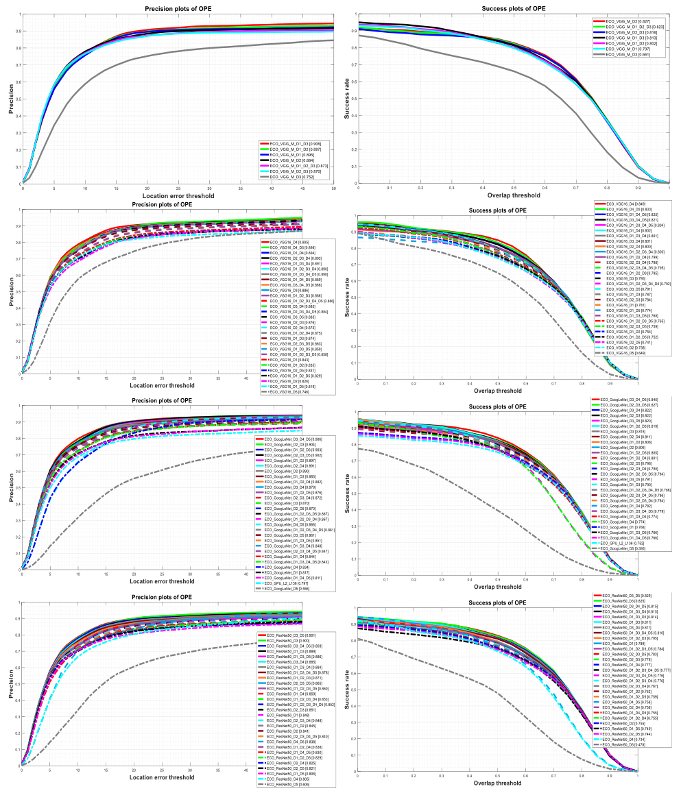
In the following, the results of proposed comprehensive analysis of four pre-trained CNN models are presented. In fact, Table 4 and Table 5 are summarized the best overall and attribute-based analyses of the ones in this appendix. In the following, Fig. 6 compares the overall precision and success rates of modified ECO tracker, which employs the VGG-M Chatfield et al. 2014, VGG-16 Simonyan and Zisserman 2014, GoogLeNet Szegedy et al. 2015, and ResNet-50 He et al. 2016 for feature extraction. According to Fig. 1, two attribute dictionaries are formed, which allow the DCF-based trackers to exploit deep features, adaptively.

Table 7: Success analysis results for pre-trained VGG-M model on OTB-2013 dataset.

Layers	Features: Resolution/Depth	Attributes
		Object				Camera				Environment
		SV	DEF	OPR	IPR	FM	MB	LR	OV	BC	OCC	IV
D1	109x109 / 96	0.727	0.831	0.759	0.713	0.741	0.754	0.598	0.840	0.719	0.807	0.752
D2	26x26 / 256	0.752	0.891	0.798	0.727	0.787	0.799	0.659	0.901	0.752	0.856	0.752
D3	13x13 / 512	0.645	0.643	0.644	0.610	0.639	0.687	0.383	0.599	0.620	0.700	0.591
D1, D2	MR / 352	0.737	0.879	0.774	0.697	0.797	0.824	0.694	0.858	0.728	0.844	0.763
D1, D3	MR / 608	0.756	0.841	0.780	0.732	0.801	0.829	0.701	0.931	0.749	0.840	0.783
D2, D3	MR / 768	0.766	0.826	0.784	0.718	0.799	0.807	0.672	0.913	0.746	0.831	0.742
D1, D2, D3	MR / 864	0.751	0.866	0.793	0.729	0.787	0.806	0.660	0.905	0.736	0.871	0.738

Table 8: Precision analysis results for pre-trained VGG-M model on OTB-2013 dataset.

Layers	Features: Resolution/Depth	Attributes
		Object				Camera				Environment
		SV	DEF	OPR	IPR	FM	MB	LR	OV	BC	OCC	IV
D1	109x109 / 96	0.860	0.903	0.891	0.846	0.804	0.808	0.594	0.848	0.815	0.898	0.837
D2	26x26 / 256	0.841	0.916	0.874	0.814	0.816	0.783	0.673	0.894	0.785	0.913	0.812
D3	13x13 / 512	0.738	0.724	0.764	0.734	0.677	0.731	0.377	0.561	0.697	0.762	0.705
D1, D2	MR / 352	0.874	0.919	0.901	0.837	0.855	0.847	0.702	0.860	0.827	0.939	0.845
D1, D3	MR / 608	0.884	0.905	0.905	0.862	0.855	0.855	0.711	0.927	0.850	0.928	0.872
D2, D3	MR / 768	0.848	0.871	0.856	0.789	0.823	0.792	0.669	0.897	0.788	0.884	0.813
D1, D2, D3	MR / 864	0.818	0.872	0.861	0.797	0.814	0.788	0.670	0.896	0.793	0.924	0.778

Table 9: Success analysis results for pre-trained VGG-16 model on OTB-2013 dataset.

Layers	Features: Resolution/Depth	Attributes
		Object				Camera				Environment
		SV	DEF	OPR	IPR	FM	MB	LR	OV	BC	OCC	IV
D1	224x224 / 64	0.735	0.769	0.751	0.699	0.688	0.687	0.567	0.736	0.691	0.785	0.714
D2	112x112 / 128	0.711	0.709	0.684	0.634	0.719	0.733	0.667	0.837	0.665	0.751	0.668
D3	56x56 / 256	0.742	0.841	0.756	0.689	0.755	0.766	0.678	0.858	0.721	0.830	0.727
D4	28x28 / 512	0.792	0.893	0.836	0.778	0.822	0.818	0.671	0.924	0.775	0.889	0.772
D5	14x14 / 512	0.637	0.609	0.639	0.619	0.653	0.635	0.398	0.609	0.542	0.647	0.668
D1, D2	MR / 192	0.679	0.789	0.705	0.647	0.685	0.680	0.560	0.743	0.652	0.779	0.663
D1, D3	MR / 320	0.731	0.827	0.747	0.684	0.735	0.737	0.687	0.855	0.703	0.819	0.717
D1, D4	MR / 576	0.736	0.852	0.766	0.722	0.741	0.778	0.700	0.759	0.738	0.835	0.728
D1, D5	MR / 576	0.732	0.765	0.733	0.660	0.701	0.725	0.597	0.776	0.726	0.780	0.724
D2, D3	MR / 384	0.725	0.820	0.742	0.678	0.730	0.731	0.687	0.863	0.706	0.819	0.713
D2, D4	MR / 640	0.733	0.831	0.764	0.702	0.770	0.771	0.705	0.880	0.722	0.843	0.732
D2, D5	MR / 640	0.700	0.747	0.691	0.612	0.688	0.685	0.591	0.734	0.678	0.756	0.677
D3, D4	MR / 768	0.730	0.854	0.764	0.723	0.739	0.795	0.710	0.775	0.744	0.818	0.715
D3, D5	MR / 768	0.739	0.824	0.755	0.689	0.760	0.769	0.673	0.824	0.716	0.830	0.731
D4, D5	MR / 1024	0.793	0.846	0.816	0.779	0.822	0.807	0.644	0.913	0.731	0.869	0.739
D1, D2, D3	MR / 448	0.739	0.828	0.757	0.694	0.752	0.754	0.691	0.865	0.723	0.833	0.732
D1, D2, D4	MR / 704	0.733	0.841	0.762	0.695	0.758	0.762	0.702	0.865	0.727	0.841	0.732
D1, D2, D5	MR / 704	0.709	0.764	0.705	0.618	0.707	0.707	0.628	0.784	0.705	0.773	0.699
D1, D3, D4	MR / 832	0.741	0.849	0.764	0.701	0.762	0.772	0.705	0.884	0.721	0.839	0.736
D1, D3, D5	MR / 832	0.730	0.779	0.725	0.650	0.749	0.756	0.701	0.839	0.708	0.787	0.724
D1, D4, D5	MR / 1078	0.766	0.845	0.796	0.733	0.805	0.797	0.704	0.894	0.752	0.886	0.762
D2, D3, D4	MR / 896	0.747	0.836	0.760	0.706	0.772	0.778	0.713	0.886	0.707	0.830	0.730
D2, D3, D5	MR / 896	0.727	0.764	0.720	0.641	0.750	0.757	0.669	0.771	0.708	0.776	0.721
D3, D4, D5	MR / 1280	0.755	0.856	0.790	0.735	0.770	0.770	0.713	0.875	0.743	0.856	0.747
D1, D2, D3, D4	MR / 960	0.735	0.839	0.763	0.698	0.762	0.758	0.710	0.884	0.723	0.840	0.744
D1, D2, D3, D5	MR / 960	0.720	0.771	0.717	0.647	0.731	0.731	0.672	0.846	0.703	0.785	0.716
D2, D3, D4, D5	MR / 1408	0.759	0.803	0.756	0.686	0.790	0.791	0.711	0.878	0.741	0.830	0.763
D1, D3, D4, D5	MR / 1344	0.756	0.812	0.767	0.730	0.775	0.777	0.707	0.865	0.702	0.828	0.710
D1, D2, D3, D4, D5	MR / 1472	0.757	0.795	0.752	0.689	0.788	0.788	0.714	0.871	0.735	0.821	0.757

Table 10: Precision analysis results for pre-trained VGG-16 model on OTB-2013 dataset.

Layers	Features: Resolution/Depth	Attributes
		Object				Camera				Environment
		SV	DEF	OPR	IPR	FM	MB	LR	OV	BC	OCC	IV
D1	224x224 / 64	0.807	0.810	0.835	0.775	0.747	0.704	0.560	0.757	0.760	0.847	0.771
D2	112x112 / 128	0.801	0.770	0.802	0.736	0.786	0.785	0.691	0.838	0.783	0.849	0.753
D3	56x56 / 256	0.861	0.886	0.879	0.819	0.817	0.788	0.676	0.842	0.824	0.915	0.822
D4	28x28 / 512	0.877	0.921	0.905	0.853	0.861	0.855	0.729	0.934	0.833	0.944	0.850
D5	14x14 / 512	0.752	0.701	0.750	0.715	0.710	0.691	0.453	0.593	0.608	0.731	0.665
D1, D2	MR / 192	0.772	0.826	0.813	0.747	0.761	0.685	0.559	0.750	0.754	0.863	0.727
D1, D3	MR / 320	0.842	0.885	0.865	0.801	0.783	0.745	0.703	0.857	0.799	0.895	0.799
D1, D4	MR / 576	0.862	0.904	0.887	0.851	0.808	0.829	0.723	0.772	0.839	0.927	0.816
D1, D5	MR / 576	0.780	0.784	0.794	0.719	0.732	0.729	0.598	0.762	0.768	0.814	0.754
D2, D3	MR / 384	0.844	0.885	0.867	0.804	0.784	0.747	0.702	0.857	0.799	0.907	0.800
D2, D4	MR / 640	0.829	0.856	0.864	0.802	0.812	0.777	0.722	0.881	0.809	0.928	0.782
D2, D5	MR / 640	0.813	0.785	0.812	0.731	0.759	0.736	0.607	0.746	0.784	0.853	0.750
D3, D4	MR / 768	0.849	0.906	0.879	0.841	0.796	0.815	0.732	0.783	0.824	0.917	0.808
D3, D5	MR / 768	0.862	0.887	0.880	0.815	0.819	0.787	0.670	0.808	0.827	0.913	0.824
D4, D5	MR / 1024	0.879	0.898	0.895	0.855	0.855	0.839	0.704	0.921	0.808	0.932	0.829
D1, D2, D3	MR / 448	0.862	0.885	0.879	0.819	0.819	0.797	0.706	0.859	0.829	0.917	0.823
D1, D2, D4	MR / 704	0.830	0.855	0.864	0.802	0.809	0.777	0.723	0.880	0.808	0.926	0.780
D1, D2, D5	MR / 704	0.806	0.787	0.809	0.728	0.761	0.717	0.649	0.780	0.784	0.847	0.751
D1, D3, D4	MR / 832	0.859	0.905	0.886	0828	0.812	0.780	0.720	0.882	0.806	0.925	0.819
D1, D3, D5	MR / 832	0.852	0.836	0.848	0.775	0.791	0.754	0.716	0.837	0.805	0.871	0.805
D1, D4, D5	MR / 1078	0.853	0.861	0.881	0.822	0.853	0.838	0.725	0.899	0.835	0.954	0.809
D2, D3, D4	MR / 896	0.862	0.904	0.888	0.831	0.813	0.781	0.731	0.888	0.808	0.928	0.820
D2, D3, D5	MR / 896	0.871	0.834	0.861	0.782	0.818	0.788	0.667	0.755	0.829	0.878	0.824
D3, D4, D5	MR / 1280	0.856	0.906	0.881	0.823	0.813	0.784	0.723	0.886	0.801	0.922	0.819
D1, D2, D3, D4	MR / 960	0.859	0.902	0.885	0.827	0.803	0.775	0.725	0.882	0.803	0.923	0.814
D1, D2, D3, D5	MR / 960	0.845	0.834	0.843	0.774	0.780	0.733	0.667	0.831	0.798	0.871	0.797
D2, D3, D4, D5	MR / 1408	0.882	0.851	0.877	0.817	0.846	0.830	0.726	0.877	0.837	0.913	0.843
D1, D3, D4, D5	MR / 1344	0.860	0.905	0.883	0.826	0.808	0.780	0.722	0.881	0.800	0.925	0.817
D1, D2, D3, D4, D5	MR / 1472	0.886	0.851	0.878	0.819	0.849	0.832	0.728	0.879	0.841	0.915	0.844

Table 11: Success analysis results for pre-trained GoogLeNet model on OTB-2013 dataset.

Layers	Features: Resolution/Depth	Attributes
		Object				Camera				Environment
		SV	DEF	OPR	IPR	FM	MB	LR	OV	BC	OCC	IV
D1	112x112 / 64	0.718	0.749	0.742	0.696	0.691	0.677	0.535	0.735	0.655	0.765	0.700
D2	56x56 / 192	0.735	0.859	0.772	0.711	0.769	0.787	0.685	0.858	0.744	0.839	0.738
D3	28x28 / 256	0.767	0.879	0.786	0.711	0.762	0.756	0.526	0.778	0.715	0.843	0.732
D4	14x14 / 528	0.730	0.875	0.779	0.704	0.732	0.691	0.519	0.799	0.785	0.831	0.726
D5	7x7 / 832	0.333	0.332	0.395	0.419	0.398	0.362	0.299	0.354	0.404	0.373	0.422
D1, D2	MR / 256	0.744	0.858	0.774	0.705	0.767	0.783	0.682	0.858	0.752	0.844	0.743
D1, D3	MR / 320	0.739	0.840	0.751	0.679	0.733	0.745	0.610	0.785	0.719	0.834	0.714
D1, D4	MR / 592	0.752	0.766	0.739	0.678	0.724	0.705	0.557	0.731	0.745	0.798	0.737
D1, D5	MR / 896	0.740	0.701	0.731	0.662	0.715	0.693	0.604	0.713	0.686	0.740	0.723
D2, D3	MR / 448	0.764	0.865	0.792	0.726	0.785	0.811	0.705	0.889	0.761	0.856	0.752
D2, D4	MR / 720	0.745	0.864	0.778	0.710	0.764	0.785	0.702	0.881	0.748	0.839	0.737
D2, D5	MR / 1024	0.722	0.850	0.762	0.693	0.755	0.773	0.691	0.865	0.738	0.835	0.723
D3, D4	MR / 784	0.765	0.875	0.792	0.746	0.744	0.791	0.701	0.774	0.762	0.855	0.716
D3, D5	MR / 1088	0.770	0.876	0.789	0.718	0.761	0.737	0.539	0.790	0.712	0.845	0.730
D4, D5	MR / 1360	0.759	0.877	0.791	0.760	0.759	0.713	0.621	0.758	0.858	0.809	0.781
D1, D2, D3	MR / 512	0.760	0.866	0.788	0.720	0.784	0.804	0.693	0.874	0.761	0.854	0.754
D1, D2, D4	MR / 784	0.747	0.860	0.764	0.694	0.752	0.773	0.705	0.873	0.723	0.837	0.737
D1, D2, D5	MR / 1088	0.738	0.856	0.769	0.701	0.758	0.771	0.694	0.866	0.745	0.837	0.737
D1, D3, D4	MR / 848	0.750	0.768	0.730	0.660	0.763	0.778	0.707	0.840	0.725	0.809	0.716
D1, D3, D5	MR / 1152	0.727	0.788	0.720	0.638	0.717	0.716	0.541	0.747	0.706	0.790	0.706
D1, D4, D5	MR / 1424	0.729	0.764	0.729	0.658	0.706	0.691	0.544	0.651	0.712	0.764	0.717
D2, D3, D4	MR / 976	0.754	0.816	0.761	0.686	0.769	0.785	0.711	0.885	0.753	0.812	0.742
D2, D3, D5	MR / 1280	0.771	0.870	0.798	0.731	0.784	0.807	0.693	0.878	0.764	0.869	0.753
D3, D4, D5	MR / 1616	0.793	0.876	0.815	0.752	0.789	0.798	0.676	0.870	0.766	0.881	0.745
D1, D2, D3, D4	MR / 1040	0.751	0.810	0.743	0.665	0.763	0.772	0.691	0.865	0.728	0.807	0.734
D1, D2, D3, D5	MR / 1344	0.748	0.812	0.756	0.679	0.767	0.778	0.694	0.871	0.753	0.816	0.737
D2, D3, D4, D5	MR / 1808	0.733	0.816	0.745	0.665	0.735	0.730	0.536	0.774	0.727	0.791	0.714
D1, D3, D4, D5	MR / 1680	0.746	0.782	0.736	0.658	0.756	0.759	0.702	0.852	0.728	0.815	0.721
D1, D2, D3, D4, D5	MR / 1872	0.751	0.810	0.745	0.667	0.766	0.775	0.699	0.872	0.730	0.808	0.740

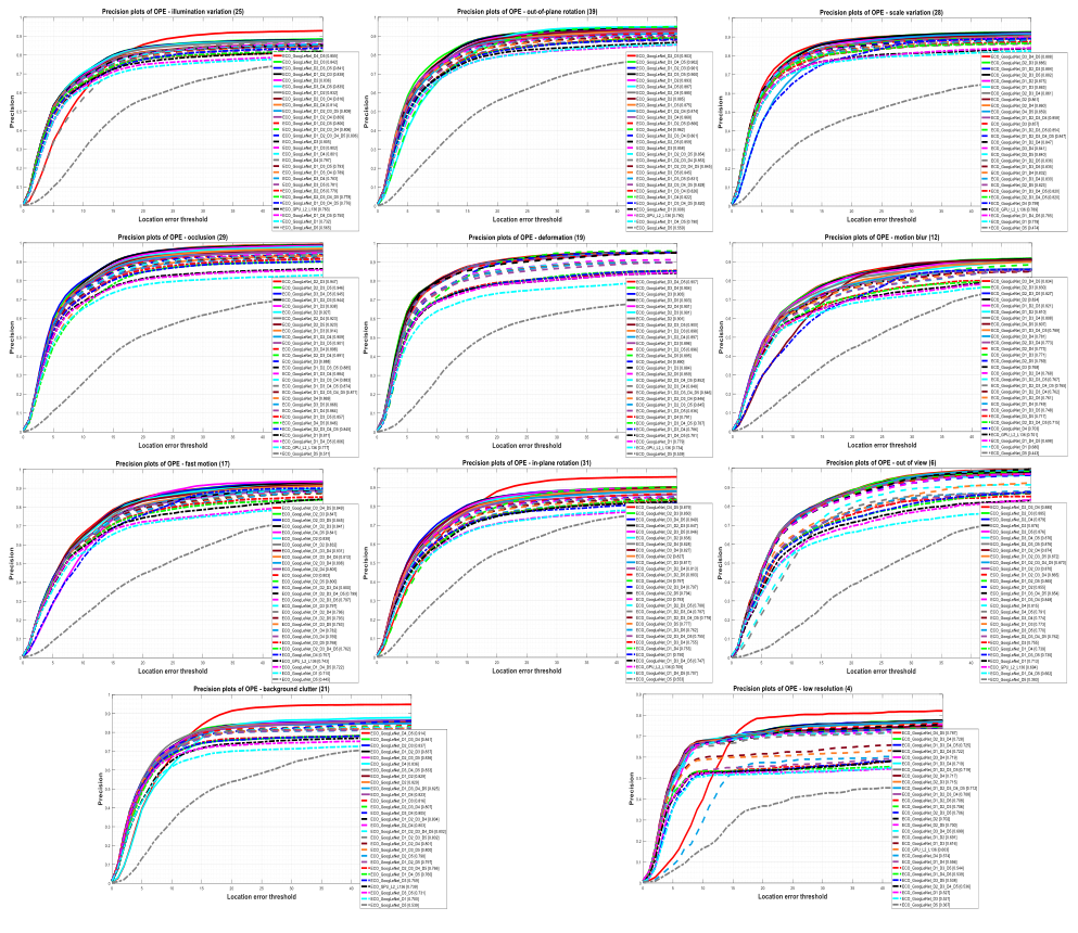
Table 12: Precision analysis results for pre-trained GoogLeNet model on OTB-2013 dataset

Layers	Features: Resolution/Depth	Attributes
		Object				Camera				Environment
		SV	DEF	OPR	IPR	FM	MB	LR	OV	BC	OCC	IV
D1	112x112 / 64	0.778	0.779	0.808	0.750	0.710	0.680	0.527	0.713	0.700	0.811	0.732
D2	56x56 / 192	0.861	0.901	0.885	0.827	0.838	0.824	0.702	0.876	0.829	0.927	0.836
D3	28x28 / 256	0.857	0.903	0.858	0.793	0.803	0.768	0.521	0.755	0.759	0.888	0.805
D4	14x14 / 528	0.799	0.890	0.862	0.797	0.757	0.703	0.574	0.815	0.836	0.869	0.797
D5	7x7 / 832	0.474	0.539	0.559	0.553	0.445	0.443	0.367	0.383	0.539	0.511	0.565
D1, D2	MR / 256	0.875	0.896	0.893	0.838	0.832	0.810	0.691	0.855	0.829	0.938	0.832
D1, D3	MR / 320	0.863	0.884	0.875	0.817	0.797	0.771	0.616	0.773	0.816	0.914	0.802
D1, D4	MR / 592	0.832	0.791	0.822	0.753	0.782	0.749	0.556	0.739	0.823	0.864	0.801
D1, D5	MR / 896	0.789	0.734	0.790	0.709	0.743	0.701	0.603	0.694	0.739	0.777	0.763
D2, D3	MR / 448	0.886	0.901	0.903	0.850	0.847	0.830	0.715	0.885	0.837	0.947	0.842
D2, D4	MR / 720	0.860	0.901	0.885	0.828	0.805	0.773	0.717	0.879	0.803	0.923	0.814
D2, D5	MR / 1024	0.823	0.859	0.859	0.794	0.800	0.769	0.700	0.876	0.798	0.920	0.779
D3, D4	MR / 784	0.841	0.904	0.868	0.827	0.769	0.781	0.719	0.774	0.805	0.898	0.783
D3, D5	MR / 1088	0.840	0.903	0.845	0.777	0.768	0.717	0.538	0.770	0.731	0.868	0.781
D4, D5	MR / 1360	0.859	0.895	0.887	0.879	0.841	0.807	0.787	0.791	0.914	0.846	0.855
D1, D2, D3	MR / 512	0.884	0.898	0.901	0.847	0.841	0.821	0.706	0.870	0.837	0.944	0.838
D1, D2, D4	MR / 784	0.847	0.897	0.874	0.813	0.796	0.768	0.722	0.874	0.801	0.909	0.809
D1, D2, D5	MR / 1088	0.836	0.896	0.866	0.803	0.793	0.761	0.708	0.865	0.797	0.901	0.806
D1, D3, D4	MR / 848	0.830	0.786	0.826	0.755	0.831	0.808	0.719	0.848	0.841	0.884	0.789
D1, D3, D5	MR / 1152	0.835	0.836	0.831	0.762	0.783	0.748	0.544	0.735	0.800	0.857	0.793
D1, D4, D5	MR / 1424	0.785	0.781	0.790	0.707	0.722	0.698	0.539	0.662	0.760	0.806	0.750
D2, D3, D4	MR / 976	0.861	0.848	0.861	0.797	0.808	0.773	0.728	0.885	0.807	0.891	0.816
D2, D3, D5	MR / 1280	0.882	0.900	0.900	0.846	0.845	0.827	0.706	0.876	0.836	0.946	0.841
D3, D4, D5	MR / 1616	0.888	0.907	0.902	0.849	0.849	0.834	0.699	0.876	0.833	0.945	0.835
D1, D2, D3, D4	MR / 1040	0.858	0.846	0.853	0.787	0.800	0.762	0.708	0.865	0.804	0.883	0.806
D1, D2, D3, D5	MR / 1344	0.854	0.845	0.854	0.788	0.797	0.767	0.719	0.872	0.802	0.885	0.809
D2, D3, D4, D5	MR / 1808	0.820	0.852	0.828	0.755	0.762	0.715	0.536	0.762	0.766	0.845	0.778
D1, D3, D4, D5	MR / 1680	0.820	0.787	0.820	0.747	0.813	0.789	0.725	0.854	0.825	0.874	0.776
D1, D2, D3, D4, D5	MR / 1872	0.847	0.846	0.845	0.778	0.799	0.765	0.712	0.870	0.802	0.871	0.806

Table 13: Success analysis results for pre-trained ResNet-50 model on OTB-2013 dataset.

Layers	Features: Resolution/Depth	Attributes
		Object				Camera				Environment
		SV	DEF	OPR	IPR	FM	MB	LR	OV	BC	OCC	IV
D1	112x112 / 64	0.741	0.799	0.759	0.719	0.704	0.707	0.597	0.707	0.691	0.787	0.725
D2	56x56 / 256	0.692	0.797	0.717	0.644	0.684	0.683	0.535	0.743	0.651	0.769	0.682
D3	28x28 / 512	0.760	0.874	0.796	0.726	0.807	0.823	0.696	0.918	0.775	0.871	0.766
D4	14x14 / 1024	0.709	0.767	0.736	0.681	0.732	0.696	0.389	0.711	0.700	0.761	0.605
D5	7x7 / 2048	0.453	0.380	0.502	0.500	0.423	0.451	0.178	0.356	0.322	0.465	0.432
D1, D2	MR / 320	0.706	0.800	0.727	0.659	0.699	0.712	0.597	0.767	0.664	0.779	0.693
D1, D3	MR / 576	0.765	0.858	0.778	0.712	0.765	0.783	0.676	0.816	0.727	0.856	0.746
D1, D4	MR / 1088	0.720	0.824	0.738	0.679	0.707	0.701	0.568	0.696	0.664	0.801	0.686
D1, D5	MR / 2112	0.667	0.811	0.698	0.671	0.629	0.678	0.530	0.527	0.631	0.750	0.625
D2, D3	MR / 768	0.748	0.807	0.735	0.655	0.749	0.762	0.667	0.830	0.723	0.799	0.727
D2, D4	MR / 1280	0.717	0.788	0.706	0.625	0.705	0.700	0.539	0.735	0.686	0.765	0.689
D2, D5	MR / 2304	0.710	0.752	0.703	0.628	0.723	0.733	0.600	0.785	0.669	0.747	0.697
D3, D4	MR / 1536	0.766	0.833	0.777	0.706	0.818	0.822	0.691	0.904	0.764	0.839	0.766
D3, D5	MR / 2560	0.766	0.883	0.801	0.735	0.816	0.830	0.704	0.930	0.762	0.871	0.763
D4, D5	MR / 3072	0.754	0.752	0.750	0.700	0.775	0.744	0.517	0.787	0.735	0.790	0.657
D1, D2, D3	MR / 832	0.745	0.853	0.757	0.686	0.748	0.760	0.673	0.834	0.718	0.828	0.726
D1, D2, D4	MR / 1344	0.716	0.792	0.705	0.624	0.700	0.701	0.536	0.725	0.689	0.763	0.687
D1, D2, D5	MR / 2368	0.716	0.783	0.711	0.630	0.718	0.708	0.600	0.785	0.701	0.772	0.705
D1, D3, D4	MR / 1600	0.762	0.864	0.783	0.717	0.777	0.771	0.688	0.848	0.723	0.864	0.751
D1, D3, D5	MR / 2624	0.756	0.862	0.782	0.716	0.781	0.789	0.708	0.858	0.733	0.864	0.754
D1, D4, D5	MR / 3136	0.735	0.708	0.709	0.672	0.716	0.721	0.613	0.719	0.667	0.736	0.685
D2, D3, D4	MR / 1792	0.725	0.786	0.721	0.648	0.739	0.739	0.551	0.753	0.690	0.780	0.708
D2, D3, D5	MR / 2816	0.753	0.804	0.741	0.663	0.758	0.782	0.679	0.843	0.745	0.810	0.740
D3, D4, D5	MR / 3584	0.769	0.837	0.782	0.710	0.829	0.843	0.708	0.940	0.772	0.847	0.777
D1, D2, D3, D4	MR / 1856	0.738	0.791	0.733	0.667	0.747	0.740	0.569	0.751	0.691	0.799	0.714
D1, D2, D3, D5	MR / 2880	0.759	0.801	0.742	0.665	0.758	0.765	0.630	0.812	0.725	0.813	0.729
D2, D3, D4, D5	MR / 3840	0.740	0.804	0.732	0.650	0.733	0.716	0.539	0.751	0.698	0.803	0.713
D1, D3, D4, D5	MR / 3648	0.754	0.850	0.777	0.719	0.780	0.777	0.714	0.860	0.707	0.856	0.742
D1, D2, D3, D4, D5	MR / 3904	0.742	0.808	0.733	0.656	0.736	0.726	0.536	0.725	0.703	0.802	0.720

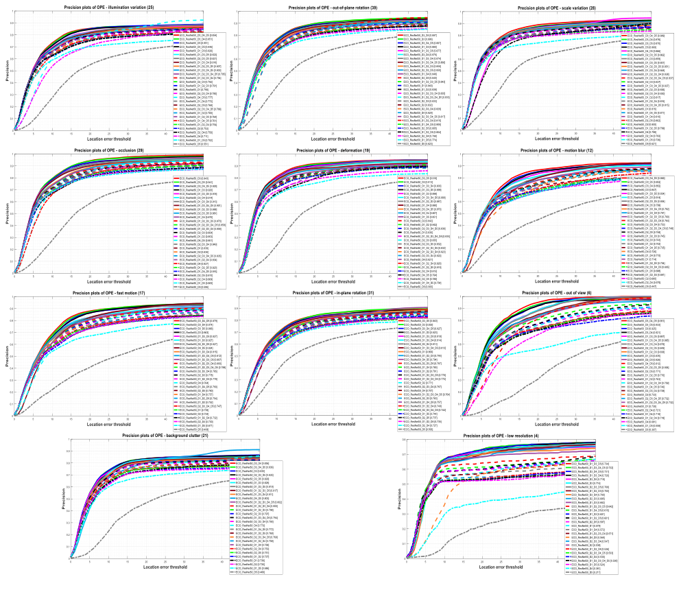
Table 14: Precision analysis results for pre-trained ResNet-50 model on OTB-2013 dataset.

Layers	Features: Resolution/Depth	Attributes
		Object				Camera				Environment
		SV	DEF	OPR	IPR	FM	MB	LR	OV	BC	OCC	IV
D1	112x112 / 64	0.815	0.836	0.840	0.800	0.738	0.714	0.579	0.730	0.736	0.839	0.790
D2	56x56 / 256	0.800	0.842	0.832	0.771	0.734	0.680	0.538	0.733	0.730	0.838	0.753
D3	28x28 / 512	0.869	0.913	0.896	0.839	0.863	0.847	0.716	0.925	0.835	0.943	0.851
D4	14x14 / 1024	0.798	0.821	0.829	0.767	0.764	0.726	0.381	0.681	0.773	0.827	0.711
D5	7x7 / 2048	0.621	0.565	0.623	0.593	0.408	0.447	0.217	0.307	0.466	0.586	0.551
D1, D2	MR / 320	0.817	0.842	0.838	0.781	0.752	0.742	0.601	0.763	0.737	0.853	0.765
D1, D3	MR / 576	0.859	0.898	0.880	0.823	0.827	0.814	0.682	0.835	0.828	0.920	0.826
D1, D4	MR / 1088	0.810	0.880	0.846	0.785	0.757	0.715	0.572	0.718	0.758	0.870	0.772
D1, D5	MR / 2112	0.736	0.851	0.774	0.744	0.671	0.688	0.524	0.558	0.686	0.805	0.702
D2, D3	MR / 768	0.837	0.835	0.833	0.763	0.778	0.743	0.685	0.826	0.797	0.854	0.792
D2, D4	MR / 1280	0.793	0.815	0.798	0.727	0.730	0.679	0.530	0.721	0.753	0.809	0.750
D2, D5	MR / 2304	0.802	0.788	0.805	0.737	0.760	0.748	0.597	0.771	0.751	0.810	0.768
D3, D4	MR / 1536	0.876	0.867	0.876	0.813	0.874	0.852	0.700	0.921	0.836	0.914	0.851
D3, D5	MR / 2560	0.870	0.918	0.897	0.840	0.866	0.852	0.719	0.933	0.829	0.941	0.846
D4, D5	MR / 3072	0.866	0.794	0.845	0.794	0.824	0.799	0.568	0.812	0.803	0.851	0.777
D1, D2, D3	MR / 832	0.836	0.887	0.858	0.795	0.778	0.745	0.700	0.838	0.798	0.888	0.791
D1, D2, D4	MR / 1344	0.816	0.820	0.815	0.749	0.732	0.681	0.536	0.718	0.758	0.834	0.754
D1, D2, D5	MR / 2368	0.799	0.819	0.804	0.735	0.754	0.704	0.601	0.770	0.769	0.823	0.764
D1, D3, D4	MR / 1600	0.848	0.903	0.874	0.814	0.815	0.781	0.720	0.879	0.811	0.913	0.816
D1, D3, D5	MR / 2624	0.851	0.899	0.877	0.819	0.827	0.834	0.734	0.887	0.819	0.918	0.823
D1, D4, D5	MR / 3136	0.811	0.754	0.808	0.757	0.760	0.735	0.615	0.740	0.772	0.816	0.761
D2, D3, D4	MR / 1792	0.830	0.822	0.829	0.767	0.785	0.753	0.547	0.738	0.790	0.849	0.785
D2, D3, D5	MR / 2816	0.862	0.832	0.850	0.787	0.827	0.804	0.708	0.849	0.835	0.881	0.821
D3, D4, D5	MR / 3584	0.889	0.870	0.887	0.827	0.879	0.866	0.731	0.951	0.836	0.929	0.854
D1, D2, D3, D4	MR / 1856	0.838	0.823	0.835	0.775	0.800	0.764	0.571	0.759	0.800	0.858	0.794
D1, D2, D3, D5	MR / 2880	0.851	0.832	0.843	0.778	0.807	0.780	0.642	0.806	0.817	0.870	0.807
D2, D3, D4, D5	MR / 3840	0.815	0.836	0.817	0.744	0.747	0.695	0.533	0.732	0.769	0.835	0.768
D1, D3, D4, D5	MR / 3648	0.837	0.888	0.866	0.813	0.812	0.782	0.732	0.885	0.794	0.901	0.803
D1, D2, D3, D4, D5	MR / 3904	0.837	0.835	0.833	0.764	0.788	0.748	0.530	0.732	0.802	0.859	0.795