Statistical Mechanics of Active Ornstein Uhlenbeck Particles
Abstract
We study the statistical properties of Active Ornstein Uhlenbeck particles (AOUPs). In this simplest of models, the Gaussian white noise of overdamped Brownian colloids is replaced by a Gaussian colored noise. This suffices to grant this system the hallmark properties of active matter, while still allowing for analytical progress. We study in detail the steady-state distribution of AOUPs in the small persistence time limit and for spatially varying activity. At the collective level, we show AOUPs to experience motility-induced phase separation both in the presence of pairwise forces or due to quorum-sensing interactions. We characterize both the instability mechanism leading to phase separation and the resulting phase coexistence. We probe how, in the stationary state, AOUPs depart from their thermal equilibrium limit by investigating the emergence of ratchet currents and entropy production. In the small persistence time limit, we show how fluctuation-dissipation relations are recovered. Finally, we discuss how the emerging properties of AOUPs can be characterized from the dynamics of their collective modes.
I Introduction
The hallmark of activity is the lack of connection at the microscopic scale between the injection of energy and its dissipation. While the latter is provided by the environment which, like for an equilibrium colloidal particle, can be an equilibrated liquid, the former arises from the consumption of an independent energy source, whose origin varies from systems to systems. In biology, energy injection typically results from the hydrolysis of ATP, which drives almost all biological processes such as cell motion Saw et al. 2017; Kawaguchi et al. 2017 or intracellular trafficking Guo et al. 2014; Ahmed et al. 2018. Synthetic active particles, on the other hand, have been powered using a large range of external sources, whose natures range from chemical Howse et al. 2007; Palacci et al. 2010; Volpe et al. 2011 to electrical Bricard et al. 2013; Nishiguchi and Sano 2015; van der Linden et al. 2019; Yan et al. 2016 to mechanical Volfson et al. 2004; Narayan et al. 2007; Deseigne et al. 2010.
At a theoretical level, the modelling of active systems has been equally diverse, starting either at a coarse-grained, phenomenological level Toner and Tu 1995; Kruse et al. 2004; Marchetti et al. 2013; Wittkowski et al. 2014 or directly at the microscopic scale, using various models of self-propelled particles Vicsek et al. 1995; Cates 2012; Romanczuk et al. 2012; Fodor and Marchetti 2018. In the latter case, the standard dynamics of self-propelled particles typically writes, ignoring inertial effects, as
| (1) |
where describes the position of particle , its self-propulsion velocity, the particle mobility, and we have included a putative interaction potential . The type of active particles is then specified by the properties of their self-propulsions . The most studied examples are probably run-and-tumble particles (RTPs) Schnitzer 1993 and active Brownian particles (ABPs) Fily and Marchetti 2012, for which has a constant modulus and reorient either stochastically at a given rate for RTPs or following rotational diffusion for ABPs. These microscopic models and their variants have led to a wealth of surprising behaviours, among which the accumulation at hard boundaries Elgeti and Gompper 2009; Tailleur and Cates 2009, the generation of currents by asymmetric obstacles Galajda et al. 2007; Tailleur and Cates 2009; Di Leonardo et al. 2010; Sokolov et al. 2010; Koumakis et al. 2014; Pietzonka et al. 2019, the emergence of collective motion Vicsek et al. 1995; Grégoire and Chaté 2004, and motility-induced phase separation (MIPS) Tailleur and Cates 2008; Fily and Marchetti 2012; Cates and Tailleur 2015.
Whatever the microscopic non-equilibrium origin of self-propulsion, these rich behaviors would be impossible if the ’s were well described by Gaussian white noises, which would make Eq. (1) an equilibrium dynamics. ABPs and RTPs differ from this simpler case by both the non-Gaussian nature and the persistence of their self-propulsion. Over the past few years, a desire to pinpoint the fundamentals of active matter has led to study simplified models, in which only the non-Gaussian nature Fodor et al. 2018 or the persistence Szamel 2014; Maggi et al. 2015; Marini Bettolo Marconi and Maggi 2015; Szamel et al. 2015; Farage et al. 2015; Fodor et al. 2016; Wittmann et al. 2017a; Wittmann et al. 2017b; Marini Bettolo Marconi et al. 2017; Caprini et al. 2019a; Caprini et al. 2019b is retained. In this article, we consider the latter case, referred to as Active Ornstein-Uhlenbeck particles (AOUPs), which, besides their theoretical motivations, have also been used to model the motion of passive tracers in an active bath of bacteria Maggi et al. 2014; Koumakis et al. 2014 as well as for the collective dynamics of cells Deforet et al. 2014; Hakim and Silberzan 2017.
The self-propulsion velocities of AOUPs are given by independent Ornstein-Uhlenbeck processes:
| (2) |
where forms a set of zero-mean Gaussian white noises with correlations , with Greek indices running over spatial dimensions. It follows that forms a set of zero-mean colored Gaussian noises with correlations
| (3) |
where controls the noise amplitude, and quantifies the noise persistence. In the limit of vanishing , the self-propulsion velocities reduce to Gaussian white noises of correlation . For finite , on the contrary, the temporal correlations of the ‘active noise’ are not matched by a corresponding memory kernel for the instantaneous damping , so that Eq. (1) does not satisfy a FDT of the second kind: it describes a non-thermal process Berthier and Kurchan 2013. The correlation time hence controls the nonequilibrium properties of the dynamics.
In this article, we study AOUPs both at single-particle and collective levels, and we characterize their static properties as well as their non-equilibrium dynamical features. In section II, we first discuss various limiting cases in which the steady-state distributions of AOUPs can be computed analytically. We discuss in particular the small-persistence-time regime, as well as the impact of non-uniform persistence and activity on the spatial distribution of particles. In section III, we show that AOUPs can undergo MIPS, both in the presence of pairwise purely repulsive forces and due to quorum-sensing interactions if the typical velocity, , is a sufficiently strongly decreasing function of the local particle density. In section IV, we then turn to characterize dynamically the departure from equilibrium of AOUPs. We first consider the occurence of particle currents in the presence of ratchet potentials and we then fully characterize the breakdown of time-reversal symmetry. At linear order in , we show AOUPs to admit an effective, non-Boltzmann equilibrium regime, which we characterize dynamically in section V by deriving the corresponding generalized fluctuation-dissipation theorem (FDT). Finally, we discuss in section VI the explicit coarse-graining of interacting AOUPs by constructing the dynamics of their collective modes. Note that sections II.1, IV.2, and V.1 correspond to detailed presentations of results announced in Fodor et al. 2016 while section II.3 is a short review on the application of UCNA and Fox theory to AOUPs. All other sections correspond to new material.
II Steady state distribution
This section is devoted to the analytical characterization of the stationary distribution of AOUPs. We begin in II.1 with the short-persistent-time regime, which has attracted a lot of interest recently Maggi et al. 2015; Marini Bettolo Marconi and Maggi 2015; Farage et al. 2015; Fodor et al. 2016; Wittmann et al. 2017a; Wittmann et al. 2017b; Marini Bettolo Marconi et al. 2017; Caprini et al. 2019a; Caprini et al. 2019b; Bonilla 2019. We present an expansion to second order in and show in II.2 how, for a single degree of freedom, it can be extended to higher order. The gap with standard methods developed to characterize the steady-state of particles powered by Gaussian colored noises Fox 1986a; Fox 1986b; Jung and Hänggi 1987; Cao et al. 1993 is then bridged in II.3. Finally, the steady-state of AOUPs with spatially varying activity and persistence is discussed in II.4. Note that sections II.1-II.3 are detailed derivations of the results presented in Fodor et al. 2016, especially for the steady-state distribution Eq. (18), and discussions of these results with respect to the existing literature; their content is mostly technical and they can be omitted during a first reading of the article.
II.1 Systematic perturbative derivation
Let us start by introducing the particle velocities to recast the dynamics of interacting AOUPS into:
| (4) |
where the mobility has been set to unity. Setting in both sides of Eq. (4) leads to the standard overdamped equilibrium dynamics:
| (5) |
Note that setting only in the right-hand side of Eq. (4) also leads to an equilibrium process: the underdamped Kramers equation. More surprisingly, setting in the left-hand side of Eq. (4) also leads to an equilibrium dynamics, albeit with non-trivial mobility and effective potential Maggi et al. 2015. This path will be detailed in II.3 and we now discuss how a small expansion of (4) can instead be systematically derived.
Here we follow the treatment introduced in Fodor et al. 2016 which works with the variables. In the spirit of Doering et al. 1987; Jung and Hänggi 1987, we first introduce the scaled variables and . As a result, the stationary distribution satisfies , where the operator reads
| (6) | ||||
Here, and in the following, summations over repeated indices are implicit. (This includes terms like or .) To compute the stationary distribution, we propose the following ansatz:
| (7) |
where, for convenience, we define and , and we introduce the notation , which lightens the notations in the many-particle case. Note that, for normalization purposes, has to vanish. We then obtain a set of recursive equations for the equating every order in
| (8) |
where
| (9) |
Inspection of (8) suggests an ansatz for the in the form of degree- polynomials in the momenta. (If this is assumed for with , then is a polynomial of degree .) It can be also checked that contains only even terms in the momenta and only odd ones. This results from the symmetry of the equation under the transformation . We use the following notation
| (10) | ||||
where the ’s depend on the particles’ positions. Note that contains a -independent term only if is even. Note also that (10) is a local function of the momenta, which could be restrictive, but still allow for non-local dependence on the particle positions, something known to be important for active particles Van den Broeck and Hänggi 1984; Solon et al. 2015.
Plugging the expression (10) for in (8), and equating order by order in , yields explicit expressions of all tensors for . For even , this leaves unconstrained (whereas by definition) but constrains . For instance, we get for :
| (11) | ||||
| (12) | ||||
| (13) |
The lowest order in of Eq. (8) for of the form (10) also yields
| (14) |
where are functions of the particle positions which can be computed explicitly. Finding a solution to (14) thus provides a closed expression for the expansion up to order .
From the Fredholm alternative theorem, the condition under which (14) admits a solution, and the expansion can be carried out, is that is orthogonal to Fredholm 1903. This is always possible in the small limit, following Bouchet et al. 2016, but the existence of solution to arbitrary order remains, in the general case, an open problem. Here we show that it can be carried out explicitly up to order . indeed reads
| (15) | ||||
and (14) is solved, for , by
| (16) |
This yields the following expression for the stationary measure of interacting AOUPs, valid up to order ,
| (17) | ||||
The velocity distribution obtained by integrating over the particle position is Gaussian to first order in , with the same variance as in Marconi et al. 2016, obtained within the UCNA framework that we discuss in Section II.3. However, the order shows that the velocity distribution is non-Gaussian to this order.
Integrating over velocities, we obtain the many-body marginal distribution, in position space, :
| (18) |
We can now use expression (18) to define an effective potential through which provides an intuitive picture of how self-propulsion affects the bare steady-state . The correction term is always positive, irrespective of the repulsive or attractive nature of the force : it drives particles away from regions of large forces. The second correction term is dominant for large values of and can take either sign. It favors the presence of particles in convex potential landscapes. When the bare potential describes pairwise interactions, the corresponding effective potential contains three-body interactions stemming from the term . Moreover, when corresponds to repulsive interactions only, the associated combines repulsive and attractive interactions Farage et al. 2015; Marini Bettolo Marconi and Maggi 2015. This captures how self-propulsion produces attractive effects out of repulsive forces, consistently with the enhanced tendency towards clustering reported experimentally for various colloidal systems Theurkauff et al. 2012; Palacci et al. 2013; Buttinoni et al. 2013; Io et al. 2017; Geyer et al. 2019.
It is interesting to note that similar functional forms to (17) and (18) are encountered in many contexts, from the semi-classical expansion of the Boltzmann distribution in powers of LANDAU and LIFSHITZ 1980 to the Hermitian form of the Fokker-Planck operator Van Kampen 1992. It would be interesting to know whether this is just a coincidence or reflects the presence of a deeper connection.
II.2 One particle in one dimension
The systematic perturbative expansion presented in Sec. II can be carried out to any order in in the case of a single AOUP particle in for an arbitrary smooth external potential in an infinite space. In this case the solvability conditions (14) admits a solution to arbitrary order , explicitly given by
| (19) |
where is a constant to be fixed by the normalization of the stationary measure. In this case, the solution can be obtained iteratively to arbitrary order, at the cost of expressions of increasing complexity. The result of this procedure is illustrated in Appendix A where we give the full stationary distribution ) up to order . Once the velocity is integrated out, we find:
where refers to the -order derivative of . Interestingly, this result is compatible with a recent, instanton-based derivation of the steady-state of AOUPs obtained sending before taking the limit Woillez et al. 2019. (Naturally, in this limit, only the terms proportional to in Eq. (II.2) survive.)
The case with periodic boundary condition is discussed in Appendix A. Furthermore, the perturbation expansion can also be generalized to the case of one particle in a central potential in arbitrary dimension, as well as to the case of two interacting particles with central forces. (We leave these cases to future works.)
Let us take advantage of working in a simpler, one-dimensional context to address more subtle questions regarding the nature of our small expansion (7). It is for instance natural to ask whether this series admits a finite convergence radius in . Equation (7) indeed implicitly assumes that is analytic in which need not necessarily hold for any potential.
To address this question, we consider the potential , at fixed and for two different values of , and consider the marginal in space of the full distribution:
| (20) |
where and is defined in (7). Truncating this series at order , we show in Fig. 1a that the truncation seems well behaved for , yielding a precise quantitative agreement with the stationary distribution obtained numerically. Note that the distribution develops symmetric humps which highlight the non-Boltzmann nature of the stationary state. For , Fig 1c shows that successive orders of the expansion are typical of an asymptotic series: each order in contributes a larger amount than the previous one with large positive and negative oscillations. This need not mean that the full series fails at capturing the steady state, but simply that finite sums yield poor approximations of the full series. An alternative procedure to estimate a series out of the asymptotic series of partial sums is to use Borel resummation. To do so, we use the method of Pade approximants. We begin by introducing the Borel transformed series
| (21) |
and we approximate as rational fractions , where and are polynomials in of order such that and coincide up to order . The series (20) can then be evaluated from the Laplace transform of : . The limit of as is called the Borel resummation of Serone et al. 2017. We first show in Fig. 1b that, when the series (20) is well approximated by its partial sum, it is (reassuringly) also well described by its truncated Borel sum. More interestingly, for , when the partial sums seem to diverge, the Borel resummation of (20) still agrees quantitatively with numerical estimates of the steady-state distribution, as shown in Fig. 1d.
II.3 Approximate dynamics: unified colored noise and Fox approximations
Approximate treatments of the dynamics (4) have been proposed in the past, based on schemes initially developed for non-interacting particles. They are usually referred to as the unified colored-noise approximation (UCNA) Jung and Hänggi 1987; Cao et al. 1993 and the Fox theory Fox 1986a; Fox 1986b. These approximations were first motivated by the description of the fluctuations of the radiation in the dye laser Jung and Hänggi 1988; Cao et al. 1993. They have, in particular, been used to determine approximations of the stationary distribution of dynamics (4) and of mean first-passage times Fox 1988; Bray and McKane 1989; Bray et al. 1990; Hanggi and Jung 1995.
The UCNA consists in neglecting the left-hand side in Eq. (4):
| (22) |
where , and we have introduced the tensor . As a result, the dynamics is now Markovian for the particle positions, at the cost of a position-dependent damping matrix . The derivation of Eq. (22) yields an equation which is to be understood with the Stratonovich convention Hanggi and Jung 1995. It follows that the associated Fokker-Planck equation for reads
| (23) | ||||
where denotes the inverse of . A simple derivation of the corresponding stationary distribution is detailed in Appendix B, and leads to Maggi et al. 2015; Marconi et al. 2016
| (24) |
The stationary distribution differs from the equilibrium Boltzmann distribution , which is recovered in the limit. The distribution (24) can be simplified to yield (18), showing it to coincide with our perturbative treatment to first order in . Note, however, that Appendix B shows that UCNA maps the AOUPs dynamics onto an equilibrium one, satisfying detailed balance with respect to the steady-state distribution (24). As such, it will be unable to capture any non-equilibrium dynamical effects, from the emergence of currents in ratchet potentials to non-vanishing entropy production.
The Fox theory uses projection methods to derive an approximate Fokker-Planck description of the dynamics of AOUPs Faetti et al. 1988; Fox 1988. In the spirit of this approach, we show in Appendix B that the approximate Fokker-Planck equation of interacting AOUPs reads, within the framework of Fox theory,
| (25) |
Note that this Fokker-Planck equation differs from that of Farage et al. 2015, as commented by Rein and Speck 2016. Again, both (25) and ref Farage et al. 2015 approximate the dynamics of AOUPs by equilibrium processes, albeit with different space-dependent mobilities and diffusivities.
Comparing (25) with the UCNA (23) show both Fokker-Planck equations to share the same probability currents up to a multiplicative factor given by . These two approximations thus yield the same stationary distribution (24), which agrees quantitatively with our perturbative result to first order in . However, both Fox and UCNA fail beyond this order. This may be seen directly by considering the order for a particle in one dimension, for which UCNA and Fox predict
| (26) |
which differs from our systematic derivation presented in Sec. II.2. Finally, we stress again that these approximation schemes both map the dynamics of AOUPs onto equilibrium ones and are thus unable to capture genuine non-equilibrium effects, unlike—as shown in Sec. IV—the expansion presented in Sec. II.1.
II.4 Spatially-varying activity
A marked difference between active and passive particles is that kinetic parameters, like the particle mobility, do not impact the steady-state distribution of passive particles, whereas they generically matter for active particles. The prototypical example is that of a spatially dependent propulsion speed , which leads to a non-uniform distribution for RTPs Schnitzer 1993; Tailleur and Cates 2008 and ABPs Tailleur and Cates 2008. This result can be directly generalized to all self-propelled particles with spatially-varying self-propulsion speeds and isotropic Markovian reorientation dynamics, whose master-equation reads Cates and Tailleur 2013
| (27) |
where is a angular vector parametrizing the -sphere in spatial dimensions, the corresponding unit vector, and is the operator accounting for the reorientation dynamics. Any isotropic reorientation process admits a uniform distribution over the sphere as a steady-state. Up to normalization issue, is thus a steady-state solution of (27), which leads to a marginal in space . Note that this accumulation in slow regions remains valid in the presence of translational diffusion, but the precise form of the steady-state now depends on the reorientation dynamics Cates and Tailleur 2015.
How this result generalizes to more complex dynamics of the self-propulsion velocity remains an open question. As we show below, AOUPs with position-dependent and also generically have non-uniform steady-states, which we characterize. We consider the following dynamics
| (28) | ||||
where and are positive functions. The corresponding master equation for the probability density is given by
| (29) |
Interestingly, introducing and maps this problem onto the dynamics of colloidal particles with inhomogeneous temperature and damping, a problem which has attracted a lot of attention in the past Van Kampen 1988a; Van Kampen 1988b; Bringuier and Bourdon 2007; Lau and Lubensky 2007; Yang and Ripoll 2013; Lim and Wehr 2019. It is then a simple exercise to check that varying and while keeping uniform leads to a Maxwellian steady-state and hence to a uniform distribution in position space . Under more general conditions, and somewhat surprisingly, Eq. (29) does not seem to admit simple steady-state solutions. As we show next, for slowly varying and , one can nevertheless show the steady-state distribution to be given by .
Integrating (29) over leads to the continuity equation
| (30) |
with . Multiplying (29) by v and integrating over v then leads to
| (31) |
where is a second-order tensor characterizing the local orientation field. Finally, the dynamics of is given by
| (32) |
where is a third-order tensor. As long as is bounded, the fields and are slaved to the density for time-scales . On such time-scales, assuming small gradients of and , Eq. (32) leads to
| (33) |
In turn, this shows the local current to take the form
| (34) |
Finally, this leads, to second order in gradient, to a diffusive dynamics for :
| (35) |
Up to normalization issues, the steady-state is then given by
| (36) |
Note that, in this approximation, the current vanishes in the steady state and is uniform in space: the spatial variations of the statistics of v are compensated by those of . Eq. (36) is illustrated numerically in Fig. 2. Eq. (35) also shows that, on the time and space scales relevant to the fast variable treatments and to the gradient expansion, AOUPs evolving with dynamics (28) are equivalent to passive particles evolving under an Itō-Langevin dynamics
| (37) |
Note that, without any approximation, Eq. (31) shows that, in the steady state, a spatially asymmetric periodic modulation of and along one space direction cannot lead to a non-vanishing current. Consider indeed one-dimensional modulations of and along, say, the direction. Equation (30) shows the current to be uniform in the steady state . By symmetry, Eq. (31) becomes in steady-state
| (38) |
Integrating over one spatial period then leads to since and is periodic. This is a surprising exception to the ratchet physics: breaking space and time symmetry may in more general cases lead to a vanishing current. Note that this extends to colloidal particles: an asymmetric modulation of the temperature along a single space direction does not lead to a steady current Van Kampen 1988a. We stress that these results hold for non-interacting particles; pairwise forces may alter this conclusion, both for active Stenhammar et al. 2016 and passive particles Van Kampen 1988a.
III Motility-Induced Phase Separation
Motility-induced phase separation is a collective phenomenon observed in self-propelled particles whose self-propulsion is hindered at high density. The particles undergo a phase separation leading to the emergence of dense phases in the absence of attractive forces, at odds with the requirements for the emergence of cohesive phases in passive systems. MIPS has been reported in experiments on self-propelled colloids Buttinoni et al. 2013; van der Linden et al. 2019 and bacteria Liu et al. 2019, where it led to a coexistence between dense arrested phases and a dilute, active, disordered gas. More recently, MIPS has been reported in a polar liquid Geyer et al. 2019 where a slow-down at high density led to the emergence of a dense macroscopic phase, which is reminiscent of traffic-jam physics Chowdhury et al. 2000; Helbing 2001; Nagatani 2002.
Self-propelled particles with persistent, non-Gaussian noises have been shown to undergo MIPS when interacting via purely repulsive pairwise forces Fily and Marchetti 2012; Redner et al. 2013; Buttinoni et al. 2013; Stenhammar et al. 2014; Wysocki et al. 2014. The resulting phase separation share similarities with the one observed for particles interacting via quorum-sensing, whose swimming speed depends on (and decreases with) the local density of particles Tailleur and Cates 2008; Cates and Tailleur 2013; Solon et al. 2015a. These sytems nevertheless display interesting differences in their mechanical and thermodynamical properties Solon et al. 2015; Solon et al. 2018a, in particular regarding the internal structure of the liquid phase Tjhung et al. 2018; Caporusso et al. 2020; Shi et al. 2020. A similar phase-separation scenario has been reported for AOUPs interacting via pairwise repulsive forces Fodor et al. 2016; Maggi et al. 2020, as well as for resembling kinetic Monte Carlo dynamics Levis and Berthier 2014; Klamser et al. 2018. This further highlights that, despite their simplicity, AOUPs retain the qualitative features of self-propelled particles at the level of collective dynamics, as was established, for instance, for the transition to collective motion Dossetti and Sevilla 2015. In this section, we bring our knowledge on MIPS in AOUPs up to par with their non-Gaussian counterparts.
We derive in section III.1 the collective hydrodynamics of AOUPs interacting via pairwise repulsive forces and analyze MIPS in this context. We highlight the similarities with the case of non-Gaussian active particles. In particular, we show that the dynamics of the density field is driven by the divergence of a generalized stress tensor. Its scaling analysis can then be used to predict a linear instability at large enough persistence, which arises from the decrease of the flux of ‘active impulse’—a concept introduced in Fily et al. 2017 and discussed in III.1.1—as the local density of particles increases. Furthermore, an equation of state for the pressure of AOUPs interacting via pairwise forces can be established. Finally, as for ABPs and RTPs Buttinoni et al. 2013; Takatori et al. 2014; Paliwal et al. 2018; Solon et al. 2018a; Arnoulx de Pirey et al. 2019; Bickmann and Wittkowski 2020, a first-principle theory of the phase diagram of AOUPs interacting via pairwise forces remains an open problem. We then show in section III.2 that AOUPs can also undergo MIPS due to quorum-sensing interactions, when the latter make their persistence times and noise amplitude depend on the local density of particles. In practice, MIPS is seen when decreases sufficiently rapidly as the local density of particles increases.
III.1 Pairwise repulsive forces
We consider AOUPs interacting via purely repulsive forces , where is a pairwise Weeks-Chandlers-Andersen (WCA) potential given by
| (39) |
when and otherwise. The dynamics of the system read
| (40) | ||||
| (41) |
For large enough , MIPS is observed and particles self-organize into dense arrested clusters which coexist with a dilute active gas (See Fig. 3).
III.1.1 Hydrodynamic equations and generalized stress tensor
To account for the underlying linear instability, we derive a hydrodynamic equation for the density field , defined as
| (42) |
where the average is taken with respect to the realization of the microscopic noises . Following step-by-step the path laid out in Solon et al. 2018a for ABPs, and thus omitting technical details, one finds that the dynamics of the density field is driven by the divergence of a current, which is given in terms of the divergence of a local ‘stress tensor’ :
| (43) |
(The mechanical interpretation of is discussed in Section III.1.3.) In noise-free, overdamped systems like the one considered here, the current in Eq. (43) is simply the particle mobility multiplied by the local force density. It may thus come as a surprise that the latter can be written as the divergence of a local tensor, despite the active, momentum-non-conserving nature of the particles.
Let us first note that the stress tensor can be split between an active and a passive part:
| (44) |
The contribution of the pairwise forces to the stress tensor is captured by , which was introduced by Irving and Kirkwood Irving and Kirkwood 1950, and whose divergence is the local force density exerted at position r:
| (45) |
This formula can be derived by symmetrizing the force density and using that Pomeau 2013; Yvon 1948
| (46) | |||
(This equality can be checked by series-expanding in powers of and integrating over , which rebuilds the Taylor expansion of in powers of .) Note that, in a system translationnally invariant along , simply measures the force density along exerted accross an interface located at position r, which endows Eq. (III.1.1) with a more direct physical interpretation.
The second contribution to the stress tensor, , is defined from:
| (47) |
Following again the path laid out in Solon et al. 2018a then leads to:
| (48) | ||||
| (49) |
Equation (49) provides a simple interpretation to : An AOUP whose self-propulsion force is at time receives an average momentum from the substrate in the future, called its ‘active impulse’ Fily et al. 2017. The underlying physical picture is that the active impulse measures the active force ‘stock’ of the particles. In Eq. (49), thus measures the flux of active impulse through the medium due to the motion of the particles, much like for ABPs and RTPs Fily et al. 2017. Equation (47) then expresses that any non-vanishing active force exerted in a volume results from the difference between inward and outward fluxes of active impulse, which measures what has been ‘spent’ to maintain a non-zero steady force.
The hydrodynamic equation (43), together with the expressions (III.1.1) and (49) for and can be used both to predict the instability of a homogeneous system at large enough persistence, as detailed in Sec. III.1.2, and to show the existence of an equation of state for the pressure, as discussed in Sec. III.1.3.
III.1.2 Scaling analysis and linear instability
To proceed, it is natural to assume, following Solon et al. 2015b, that the stress tensor is well approximated by a local equation of state . Consider a small periodic perturbation , say along the -direction, around a mean density . Equation (43) shows it to evolve as so that signals the onset of a linear instability and defines a spinodal region. To proceed further, one could approximate the various components of using local equations of states , , as was done for ABPs Solon et al. 2015b. However, direct inspection of their physical origin already captures most of the physics.
Much like for purely repulsive passive particles, vanishes in the low-density, non-interacting limit and increases monotonously until it diverges at close-packing Fisher 1965. Because particles stop when the interparticle force balances the propulsive one, the scale of is set by , where is the typical scale of the self-propulsion speed. The integral in (III.1.1) then selects the typical interaction length and the overall scaling of is
| (50) |
where the dependence on has been formally written, for dimensional reasons, as , where is a dimensionless scaling function of the rescaled density Solon et al. 2015b. (Below a crowding density , is well approximated by a linearly decaying function Fily and Marchetti 2012; Bialké et al. 2013; Solon et al. 2015; Solon et al. 2018a). Note that (50) can be derived using (III.1.1) or, equivalently, using the Virial-like formula Yang et al. 2014; Epstein et al. 2019.
Contrary to , is expected to be a non-monotonous function of . It first increases linearly with the density until interactions kick in. Because active particles collide more often with particles lying ahead than behind Bialké et al. 2013, the main effect of these interactions is to lower the flux of active impulse as the density increases, until it vanishes at close packing, leading to a non-monotonous variation of . Inspection of Eq. (49) shows the typical scale of to be
| (51) |
where is another dimensionless scaling function.
An overall decreasing stress tensor can then be observed when the decrease of is strong enough to compensate the increase of . From Eqs (50) and (51), this is realized when the rescaled persistence length is large enough:
| (52) |
Let us highlight, once again, the similarity of this criterion with that obtained for ABPs or RTPs Solon et al. 2015b.
III.1.3 An equation of state for pressure
Finally, before turning to quorum-sensing interactions, let us note that, as for other active particles interacting via pairwise forces Solon et al. 2018a, the analogy between and a stress tensor goes further than Eq. (43): it has a direct mechanical interpretation. Confining AOUPs by an external potential indeed leads to
| (53) |
with and given by (III.1.1) and (49). In a flux-free steady state, Eq. (53) shows the force density exerted by the particles on the confining boundary, , to be given by the divergence of the stress tensor . Consider a confining boundary parallel to . Integrating (53) from a point , deep in the bulk of the system, to infinity along shows the mechanical pressure exerted by the particles on the wall, , to be given by . In a bulk phase-separated system, can be equally chosen in any of the phases, showing that the pressure is identical in either of the coexisting phases.
III.2 Quorum-sensing interactions
From bacteria to self-propelled Janus colloids, many active particles experience propelling forces whose statistics depend on the composition of their environment and may thus be altered by the presence of other nearby active particles. Such mediated interactions, whether chemical, hydrodynamic or metabolic, can be modelled—somewhat crudely—by quorum-sensing (QS) interactions. These can be described using a self-propulsion whose characteristics depend on the density of neighbouring particles. Consider the dynamics of ABP or RTP, , where undergoes either rotational diffusion or a Poisson jump process, respectively. Quorum-sensing interactions can be modelled by considering a self-propulsion speed that is both a function of the position of the particle r and a functional of the density field : Solon et al. 2015a; Solon et al. 2018a; Bäuerle et al. 2018. In this context, a homogeneous phase at density has been shown to be linearly unstable to MIPS whenever Tailleur and Cates 2008; Cates and Tailleur 2013; Cates and Tailleur 2015
| (54) |
where is the self-propulsion speed of a particle in a homogeneous system at density . The role of QS for AOUPs with varying propulsion speed has not been studied so far. To fill this gap, we consider AOUPs, whose dynamics are given by and
| (55) |
where and are functions of r and functionals of the density field . In practice, we choose and where is a local smooth density field felt by a particle at position r. It is defined through
| (56) |
with a positive, symmetric kernel, normalized by and with a typical range .
III.2.1 A diffusive fluctuating hydrodynamics
We consider a long-time, large system-size limit in which the density field evolves over time-scales , where is the corresponding dynamical exponent, so that there is a clear separation between the persistence time and the time-scale of the evolution of the density field. We thus assume that the dynamics of particle is well described by its diffusive approximation. Using (37), this is given by:
| (57) |
Eq. (57) amounts to a diffusive approximation of the dynamics of the interacting AOUPs by coupled Langevin dynamics. Standard methods of stochastic calculus Dean 1996; Cates and Tailleur 2013; Solon et al. 2015a then allow one to derive a stochastic evolution equation for . Altogether, the fluctuating hydrodynamics of interacting AOUPs is given by
| (58) |
where is a Gaussian white-noise field of zero mean and unit variance.
III.2.2 Linear stability analysis of the mean-field hydrodynamics
Equation (58) is the main result of this section: it provides the fluctuating hydrodynamics of AOUPs interacting via QS through and . The structure of this equation is very similar to that of RTPs and ABPs interacting via density-dependent self-propulsion speed Cates and Tailleur 2013, but the relationship between the macroscopic transport parameters and the microscopic parameters of the self-propulsion are clearly different. The methods developed to study the collective behaviours of RTPs and ABPs interacting via QS Solon et al. 2018b; Solon et al. 2018a can be directly generalized to AOUPs. First, Eq. (58) immediately leads to an exact evolution equation for the mean density field through:
| (59) |
Note that this equations is neither closed, nor local. A further simplifying step is to implement a mean-field approximation and replace by , yielding
| (60) |
At this stage, Eq. (60) already allows one to predict the onset of a linear instability leading to MIPS. This is done by computing the linear dynamics of a perturbation around a homogeneous profile , leading to
| (61) |
where , the prime refers to a derivative with respect to , and we defined and similarly for . A Fourier transform then shows that mode relaxes with rate , where
| (62) |
The mode is unstable whenever , whence the instability criterion
| (63) |
Equation (63) defines the spinodal region of AOUPs interacting via quorum-sensing; it is the direct counterpart for AOUPs of the standard MIPS criterion (54) derived for ABPs and RTPs.
Note that Eq. (63) predicts a density-dependent persistence time to lead to MIPS whenever whereas density-dependent tumbling rates or rotational diffusion, which control the persistence times of ABPs and RTPs, do not lead to any interesting collective behaviours. The MIPS experienced by AOUPs interacting via such a density-dependent persistence time is illustrated in Figure 4.

III.2.3 Phase diagram
The full phase diagram of ABPs and RTPs interacting via quorum-sensing interactions has recently been predicted analytically by carrying out one more approximation step Solon et al. 2018b; Solon et al. 2018a. We present here a direct application of this method to AOUPs. We first recast (60) into
| (64) | |||||
| (65) |
Equation (64) shows that acts as a chemical potential. Using a second-order gradient expansion, the non-local sampling of the density field through the kernel can be written as:
| (66) |
where . This allows us to expand into
| (67) |
where
| (68) | |||||
| (69) |
Following the method laid out in Solon et al. 2018b; Solon et al. 2018a, one introduces the change of variable , solution of . This allows us to write
| (70) |
where is the generalized free energy whose local density is such that
| (71) |
The phase diagram can then be predicted, at this diffusive, mean-field level, by carrying out a common-tangent construction on . This was shown in Solon et al. 2018b; Solon et al. 2018a to give quantitative agreement with microscopic simulations as soon as is large enough that each particle interacts with many of its neighbours.
IV Emergence of time-reversal symmetry breaking
In this Section, we discuss observables which can be used to measure the deviation from equilibrium of AOUPs. First, we consider the particle current which arises spontaneously when introducing an external asymmetric potential. We obtain its expression to leading order based on the small-persistence-time expansion detailed in Sec. II. Then, we derive the entropy production rate quantifying the breakdown of time-reversal symmetry Seifert 2012. This observable has been used extensively as an unambigous nonequilibrium signature in systems driven by external fields Evans et al. 1993; Gallavotti and Cohen 1995; Kurchan 1998; Lebowitz and Spohn 1999; Maes 1999 and it has attracted a lot of attention recently in the field of active matter Speck 2016; Fodor et al. 2016; Marconi et al. 2017; Pietzonka and Seifert 2017; Mandal et al. 2017; Shankar and Marchetti 2018; Chaki and Chakrabarti 2018; Dabelow et al. 2019; Caprini et al. 2018a; Caprini et al. 2019a; Chaki and Chakrabarti 2019; GrandPre et al. 2021; Flenner and Szamel 2020. Finally, we end by discussing the symmetry of time correlations and its relation to entropy production.
IV.1 Current and Ratchet
Nonequilibrium systems can sustain currents in the steady state. One of the simplest settings for this to happen is a stochastic ratchet: a fluctuating nonequilibrium dynamics in a spatially asymmetric potential landscape generically leads to non-vanishing currents in the steady state Ajdari and Prost 1992; Magnasco 1993. Recently, several works considered active particles in asymmetric landscapes, both experimentally Galajda et al. 2007; Angelani et al. 2009; Di Leonardo et al. 2010; Sokolov et al. 2010; Kumar et al. 2019 and theoretically Wan et al. 2008; Tailleur and Cates 2009; Angelani et al. 2011; Reichhardt and Reichhardt 2017; Stenhammar et al. 2016; Pietzonka et al. 2019.
We consider here a single AOUP on a ring of length in an asymmetric potential of period . Our interest goes to the induced current in the steady state. An interesting spin-off of our computation of the stationary measure detailed in Sec. II.2 and Appendix A is a perturbative expression for . To leading order in , reads:
| (72) |
We compare in Fig. 5 the above prediction with the results of numerical simulations of an AOUP experiencing a potential . The agreement between our numerical simulations and Eq. (72) confirms the validity of our approximation at small . In particular, this is an effect that could not be captured by the UCNA or Fox approximations described in Sec. II.3: both would predict .
IV.2 Entropy production rate
To probe quantitatively the nonequilibrium properties of the dynamics, we now consider the entropy production rate Lebowitz and Spohn 1999; Seifert 2012. It is defined as the rate of (Kullback-Leibler) divergence between the probability weights associated with a given realization of the dynamics, , and its time-reversed counterpart, , respectively denoted by and , as
| (73) |
where is the length of the trajectory. The entropy production rate quantifies the irreversibility of the dynamics. Using standard path-integral formalism Onsager and Machlup 1953, the trajectory weight can be written as , where the dynamic action reads
| (74) |
We define the reversed trajectories in terms of the forward ones as
| (75) |
Note that this amounts to comparing a forward trajectory with a backward one, realized by a particle whose initial velocity is the opposite of the final velocity of the forward trajectory, a choice which has been debated Mandal et al. 2017; Caprini et al. 2018a.
From this definition, we deduce the action difference as
| (76) | ||||
where and we use the Stratonovich convention. Using , it appears that the first line in (76) integrates into a finite contribution , which does not contribute to as . We assume that the time and ensemble averages coincide under the ergodicity condition, leading us to express the entropy production rate as
| (77) |
Using the chain rule
| (78) |
and given that vanishes in steady state for any observable , we then deduce
| (79) |
The entropy production rate vanishes when is quadratic, a case which has attracted interest in the past Szamel 2014. In such a harmonic trap, AOUPs have a Gaussian, Boltzmann-like distribution, albeit with a potential-dependent “temperature”. Equation (79) shows that this quantitative difference with thermal equilibrium does not imply a breakdown of time-reversal symmetry, in the sense that detailed balance holds. The anharmonicity of the potential can thus be used as a handle to drive AOUPs out of equilibrium. Note that we use solely to detect a breakdown of time-reversal symmetry. It can also be granted a more traditional thermodynamical meaning, as recently discussed in Dabelow et al. 2019; Pietzonka et al. 2019; Ekeh et al. 2020.
Equation (79) is a global measure of the entropy production rate over the whole system. We now turn to a more detailed study of how this entropy is locally produced and, more precisely, of the spatial structures which are most sensitive to time-reversal symmetry breaking.
IV.3 Entropy production in MIPS
The relationship between MIPS and equilibrium phase-separation was initially suggested in Tailleur and Cates 2008, using a coarse-grained description only valid at the homogeneous level. Further discussions on the role of gradient terms has led to the realization that this mapping onto equilibrium is generically broken at higher order in gradients Wittkowski et al. 2014; Speck et al. 2014; Caballero et al. 2018a; Solon et al. 2018a; Tjhung et al. 2018. The entropy production of active field theories was indeed shown to be peaked at interfaces between coexisting phases Nardini et al. 2017, a result which begs to be tested in particle models.
To do so, we first construct a map of entropy production rate starting from the global formula (79) for . We consider the case where particles interact through a pair potential:
| (80) |
where to avoid self-interaction. To rewrite (79) as a sum over particle contributions, we first note that
| (81) | ||||
Using that
| (82) |
the entropy production rate can be rewritten as
| (83) |
where is given by
| (84) |
Equations (83) and (84) split the total entropy production rate into a sum of particle contributions. It is thus tempting to refer to as the entropy production rate of particle . Note, however, that we have proven neither that is positive nor that the decomposition (84) is unique. This interpretation thus has to be taken with a pinch of salt.
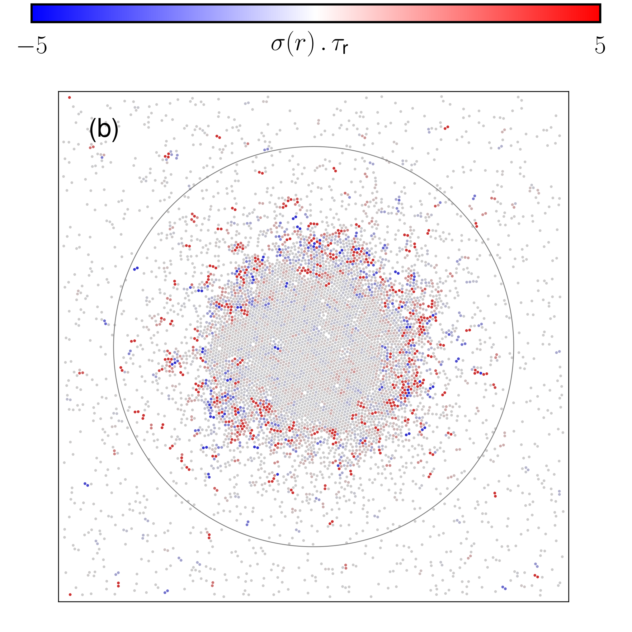
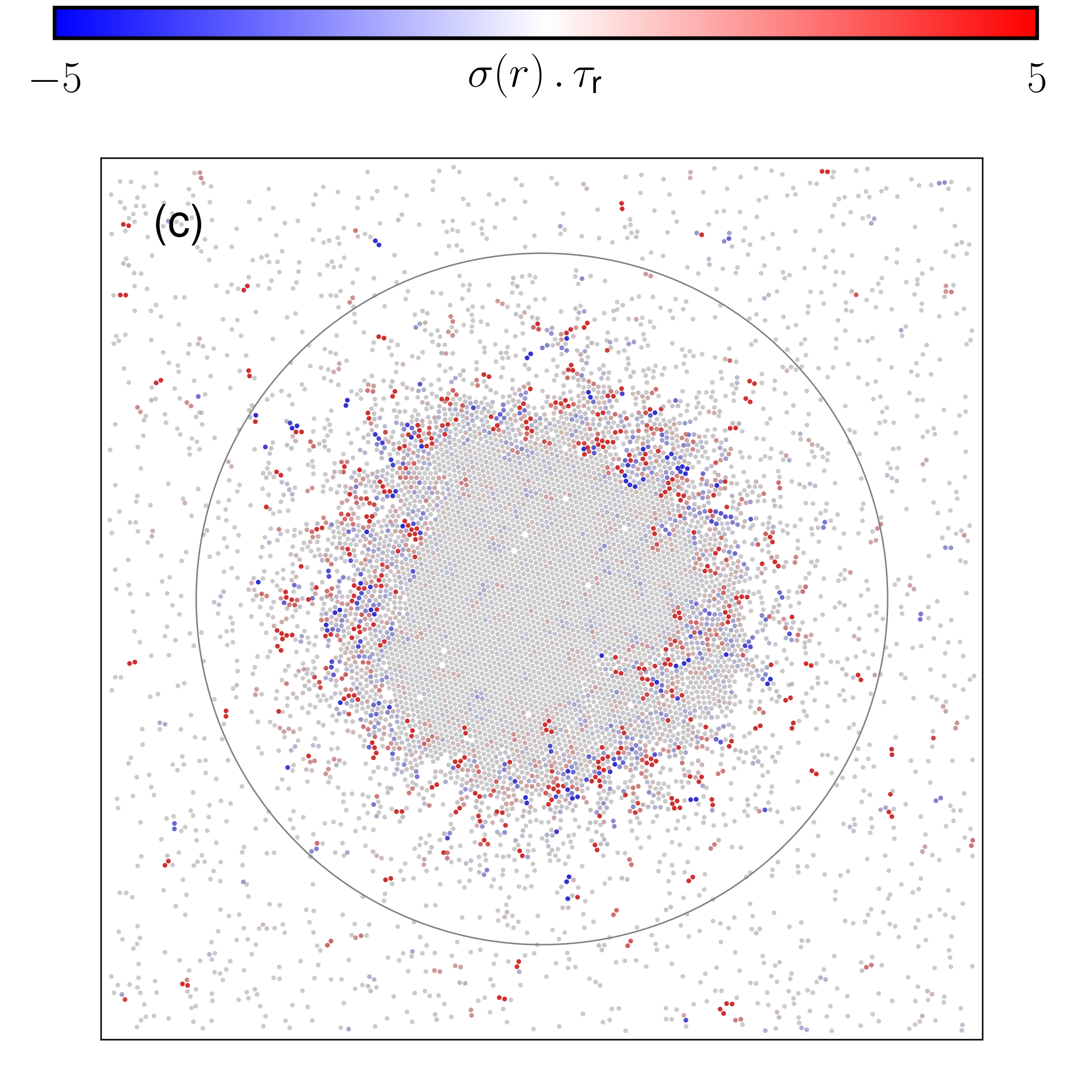
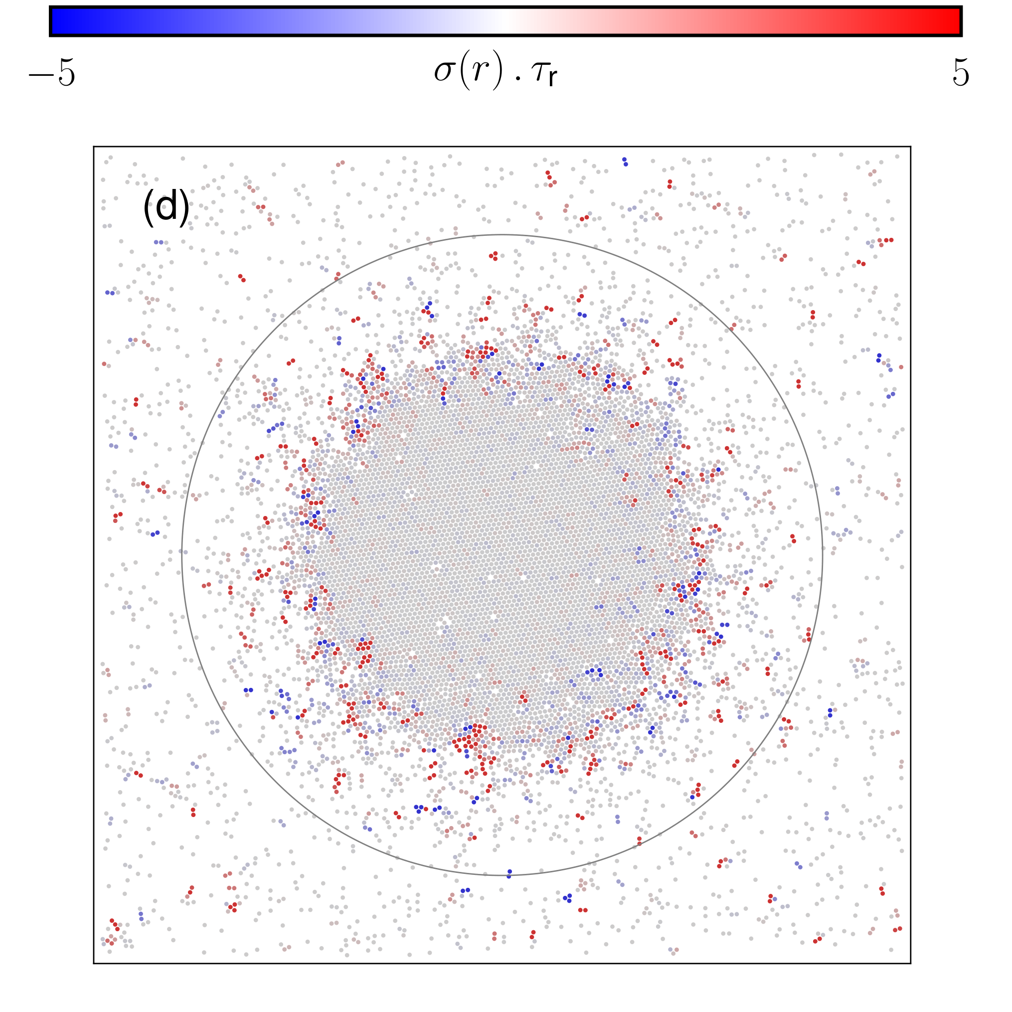
Our aim is to compute the local rate of entropy production associated with a phase-separated set of AOUPs, and in particular investigate the correlation between the structure of the density field and entropy production. We consider particles in a box, interacting via a short-range soft-core potential of the form
| (85) |
for . As discussed in Sec. III.1, such pairwise repulsive forces can lead to phase separation at high enough persistence: a macroscopic cluster of particles then forms and slowly diffuses in the system. This slow diffusion makes the comparison between the average density and the entropy production rate profiles numerically difficult and we thus pin the center of the cluster by applying a truncated harmonic trap of the form for . Note that the harmonic trap does not directly contribute to the entropy production since it is harmonic.
As show in Fig. 6 for different particle densities, a macroscopic cluster of particles indeed localizes in the center of the system and coexists with a surrounding dilute gas phase. Increasing the density mostly results in a shift of the boundary between the two phases as the cluster grows. Using Eq. (84), the contribution of each particle to the entropy production can be measured: particles in the bulk of each phase have negligible contributions whereas those localized at the boundary of the cluster exhibit large values, both positive and negative, of . To compute the net contribution to the entropy production, we construct a density of entropy production rate, where the overbar represents a binning procedure and a time average in the steady-state. The resulting profiles are shown in Fig 7, where they are compared to the density profiles.
As hinted from Fig. 6, is indeed much smaller in bulk phases than at the boundary of the dense cluster, which highlights that the breakdown of time-reversal symmetry in MIPS is dominated by interface physics. Novelty with respect to a bona fide equilibrium phase separation will thus mostly operate at the interface between dilute and dense phases, which echoes recent results on reversed Ostwald ripening and bubbly phase-separations in active systems Tjhung et al. 2018; Caballero et al. 2018b. The almost negligible value of in both bulk phases can be understood by inspection of (84): vanishes in the dense phase since the relative velocities between the particles vanish, and it reaches a small plateau value in the dilute phase, where collisions are scarce. On the contrary, reaches a maximum value at the interface where fast particles coming from the dilute phase collide onto slow ones arrested in the crowded cluster.
Note that our microscopic analysis corroborates the phenomenological coarse-grained approach of Nardini et al. 2017. This validates a posteriori the idea that, at the coarse-grained scale, the difference between MIPS and an equilibrium phase-separation lies in non-conservative gradient terms contributing mostly at the interface. Finally, the differences between all microscopic models exhibiting MIPS-like behaviours, whether on- or off-lattice, interacting via quorum-sensing or pairwise forces, should be mostly apparent, at the coarse-grained scale, in the different types of gradient terms they will generate.
IV.4 Symmetry of time correlations
While entropy production rate provides a formal estimate of the breakdown of time-reversal symmetry, its practical significance may be hard to grasp. It is furthermore not easily accessible experimentally, and its measurement has thus been carried out mostly on low-dimensional systems Andrieux et al. 2007; Roldán et al. 2018. A more pragmatic measurement of irreversibility can be inferred from the asymmetry of time-correlations of physical observables. For systems in equilibrium, time-reversibility indeed implies that time-correlations are symmetric. Consider first an overdamped equilibrium system whose configurations are specified by the positions of the particles. For any two observables and , time reversibility implies that
| (86) |
where the average is defined as
| (87) |
In (87), is the Fokker-Planck operator and the corresponding steady-state distribution.
Equation (86) can be generalized to systems with odd variables under time-reversal (), such as, for instance, underdamped dynamics. As discussed in Appendix C, considering observables and , time-reversibility now implies that
| (88) |
where and analogously for . In Eq. (88), the average is defined as in (87), albeit with the Fokker-Planck operator now acting on function defined on the full phase space. The vanishing of in Eq. (88) simply reflects that trajectories of length are as likely as the reversed ones obtained by flipping the momenta.
AOUPs possess an effective equilibrium regime, characterised by a vanishing entropy production rate for small , and we thus expect (88) to be valid in such a limit. Let us first show how the computation of and of the entropy production rate bare some similarities. Using the path-integral methods presented in section IV.2, the correlator can be written as
| (89) | |||||
where is the dynamical action defined in (74). Changing variable from to , this can be recast into
| (90) | |||||
where we have used that . Finally, using that
and dropping the superscript on the dummy variables leads to:
| (91) |
The connection to entropy production then comes from the fact that
| (92) |
We have shown in section IV.2 that the entropy production rate scales as when . Equation (91) instead involves the total entropy production during a time . Approximating the latter by would imply that as long as . This approximation is, however, uncontrolled, and one has to deal, in practice, with the boundary terms that vanish in the computation of .
In this section, we thus follow an alternative path, based on an operator formalism, that allows us to treat the small limit exactly but offers bounds on the decay of with which are weaker than those derived for . In the limit , the generator of the AOUPs process, i.e. the adjoint of the Fokker-Planck operator, is time-reversal symmetric. As increases, it develops a non-symmetric part, which can be computed using our expansion of the steady-state distribution for small . As detailed in Appendix D the leading order of the antisymmetric part of the generator is given by , where
| (93) |
and we work again with the rescaled variable . Using perturbation theory Baiesi and Maes 2013, we show in Appendix D that
| (94) | ||||
Noting that , we conclude that, for short times,
| (95) |
A stronger result than (95) actually holds when at least one of the two observables, say , depends only on positions: . In this case, indeed,
| (96) | ||||
where the first equality comes from expanding and retaining only its leading order in , , which is given by:
| (97) |
The second equality then follows by noticing that acts only on momenta. Inserting (96) in Eq. (94) leads to
| (98) |
As announced earlier, the effective time-reversal symmetry of AOUPs dynamics for small thus leads to a corresponding symmetry for two-time correlation functions. The convergence as is faster for position-dependent observables than in the full phase-space , which is consistent with the fact that momenta-like variables have to be handled with care in the context of TRS Mandal et al. 2017; Caprini et al. 2018a; Caprini et al. 2019a.
V Effective equilibrium: Linear response and fluctuation-dissipation relations
A most celebrated way of probing the nonequilibrium nature of the dynamics lies in investigating the connection between fluctuations and responses. For passive inertial Brownian particles (5), a perturbation of the potential amounts to modifying the dynamics into
| (99) |
We define the response function which measures the effect of the perturbation on the average value of an arbitrary observable as
| (100) |
Causality enforces that it vanishes when , and time-translation invariance in the steady-state means that it only depends on the time difference . In equilibrium, fluctuations and response are related by the celebrated Fluctuation Dissipation Theorem (FDT). The latter states that the response function is related to the decay rate of the (unperturbed) correlations between and :
| (101) |
Our aim is to determine to which extent one can obtain a fluctuation-dissipation relation (FDR) analogous to (101) for the active dynamics (1), a topic which has attracted interest recently Szamel 2017; Caprini et al. 2018b; Dal Cengio et al. 2019; Cengio et al. 2020; Maes 2020. These works are based on the explicit expression of the steady-state distribution of AOUPs. Here, instead, we follow Fodor et al. 2016 and proceed at a dynamical level to derive generic relations between response and correlation functions, which do not require any knowledge of the steady-state. We then study the response to perturbing the strength of self-propulsion in the effective equilibrium regime.
V.1 Perturbing with an arbitrary potential
Under the perturbation , the dynamics (1) changes as
| (102) |
To compute the response function of an observable , we write the dynamics for as
| (103) |
Using the formalism of section IV.2, the dynamical action becomes
| (104) |
The probability of a trajectory is given by , so that , leading to a response function given by
| (105) |
Note that it is sufficient to compute to first order in :
| (106) |
to determine the response function. We now follow standard procedures Cugliandolo 2011; Baiesi and Maes 2013 and we consider the difference in the steady-state where time-translation invariance means that . The difference of response functions reads
| (107) |
We now use that, due to time-translation invariance in the steady-state, for any two observables and we have . This leads to
| (108) |
Using causality, we have that, for , . Furthermore, in the effective equilibrium regime, the symmetry under a time reversal enforces that the last two lines in (108) cancel out, whereas the first two add up. All in all, the response finally reads
| (109) |
By contrast to thermal equilibrium, the response is not the time derivative of a given function in general. There are exceptions, for instance when , where are a set of constant forces exerted on the particles, as considered in Fodor et al. 2016.
The two approximate treatments presented previously, based on either UCNA or the Fox theory, lead to Markovian dynamics for the particle positions. Therefore, we can use previous results which predict the form of the response in terms of the stationary distribution Agarwal 1972; Prost et al. 2009:
| (110) |
where denotes the stationary distribution under the perturbed potential . From (24), we linearize the distribution around the unperturbed state as
| (111) | ||||
yielding
| (112) |
The result (112), which stems from the Fox theory and UCNA, differs from (109). This shows that UCNA and the Fox theory have to be used with care when studying dynamical observables, even to first order in .
V.2 Perturbing the amplitude of fluctuations
Let us now consider a perturbation in Eq. (2), which can be seen as a change in the typical self-propulsion speed at fixed persistence time. Such perturbation is particularly interesting given the recent experimental development of self-propelled particles, both of synthetic Buttinoni et al. 2013; Palacci et al. 2013; Kümmel et al. 2013; Palacci et al. 2014 and biological Walter et al. 2007; Vizsnyiczai et al. 2017; Frangipane et al. 2018; Arlt et al. 2018; Arlt et al. 2019 natures, whose self-propulsion speed can be controlled by external light sources.
Let us first recall what happens in equilibrium when perturbing the temperature, an operation we denote by . Both in the over-damped and in the under-damped cases, the effect of such a perturbation on an arbitrary observable can be written as Agarwal 1972; Baiesi et al. 2014
| (113) |
where is the energy of the system, we set the Boltzmann constant to unity, and . Here, the average is computed in the presence of the perturbation.
Let us now consider the case of AOUPs. In Appendix E, we show that a similar relation can be derived for times :
| (114) |
where
| (115) | ||||
The above result is the generalisation to AOUPs of the equilibrium result (113). Interestingly, is the effective Hamiltonian one would infer from the logarithm of the stationary measure (17) up to order . At odds with equilibrium systems where eq. (113) is valid for all times, Eq. (114) is only derived here for short trajectories.
VI Dynamics of collective modes
In this section we study the dynamics of the fluctuating microscopic density and velocity modes. They are defined in terms of the particles’ positions and velocities by
| (116) |
which are sometimes referred to as empirical measures. Neither nor are hydrodynamic fields in the sense that they are not built from a mesoscopic coarse-graining procedure. They are still fully microscopic (and as such highly singular) objects and one can thus hope to obtain exact evolution equations for them.
For particles evolving according to overdamped Langevin equations, Kawasaki and Dean have shown the steps towards an exact partial differential stochastic equation for the local density field Kawasaki 1994; Dean 1996. Extracting physical information at hydrodynamic level out of the Dean-Kawasaki equation often requires, however, a further crucial approximation: to replace with a smooth field , the hydrodynamic field, and assume that still solves the same Dean-Kawasaki equation. Indeed, it is an implicit assumption of most numerical and analytical approaches that one looks only for solutions with sufficient degree of regularity, which is assumed to have while clearly has not.
We are aware of only one case where it is possible to prove that the smoothing procedure described above is harmless, in the sense that the evolution of obeying the Dean-Kawasaki equation approximates precisely the evolution of . It happens for overdamped particles interacting with a weak potential, that scales as . This is a relevant model for either systems with long-range interactions Campa et al. 2009 such as interactions mediated by a surrounding low-Reynolds number fluid Stenhammar et al. 2017 or for very soft bodies such as polymers Doi and Edwards 1988. In this case, comparing rigorous mathematical results Dawsont and Gärtner 1987 with those obtained from the Dean-Kawasaki equation allow to conclude that captures not only the average evolution of but even its fluctuations up to those whose probability is exponentially small in Bouchet et al. 2016. For systems without weak interactions, it remains an outstanding open question the degree of approximation that is involved in passing from the empirical measure to the smooth hydrodyamic field .
In the case of systems with underdamped dynamics, a similar procedure to the one leading to the Dean-Kawasaki equation, but now involving both and , was later achieved in Nakamura and Yoshimori 2009. In this case, passing to the hydrodynamic limit would require further assumptions with respect to the case of overdamped particles, even if the equations for and appear to be closed. The main point is that, while some of the steps needed to derive closed equations for and are exactly true when working at the level of the empirical fields and , it is unclear whether they remain valid in the smoothing required to pass from them to their hydrodynamics counterparts. Taking a different approach, closure at the hydrodynamic level has been discussed by several authors up to very recently Das and Mazenko 1986; Schmitz et al. 1993; Archer 2006; Archer 2009; Das and Yoshimori 2013; Démery 2015 (see also Klymko et al. 2017; Epstein et al. 2019 for a more recent discussion within the framework of active matter).
We will not consider the issue due to passing from empirical measures to hydrodynamic fields further in what follows and concentrate instead on deriving the exact equations for and for AOUPs. These could be employed to pass to the hydrodynamic level of description and generate BBGKY-like hierarchies or implement approximation methods with no analog within the Lagrangian particle-based formulation, but their development goes beyond the scope of the present paper. We limit ourselves, at the end of the Section, to sketch future research directions along these lines.
VI.1 Fluctuating hydrodynamics
We first derive the set of equations ruling the coupled dynamics of and g. The time derivative of the local density of course takes the form of a continuity equation
| (117) |
thus expressing the conservation of the number of particles. The time derivative of the current density is given by
| (118) |
To proceed further, we assume that the particles interact through pairwise interactions only as given in (80). When substituting the microscopic dynamics (4) in the expression for the time derivative of g, a term of the following form appears:
| (119) | ||||
where the star refers to a spatial convolution, e.g. . The dynamic equation for the current density field g then follows as
| (120) | ||||
The noise term is Gaussian with correlations
| (121) |
In Eq. (120) and we have introduced a local tensor defined by
| (122) |
which can be viewed as the fluctuating analog of the kinetic part of the stress tensor (as described by Irving and Kirkwood in their seminal contribution (see Eq. (5.13) in Irving and Kirkwood 1950).
As was noted in Nakamura and Yoshimori 2009, with the additional assumption that particles are discernible or that, equivalently for classical particles, there exists a minimal hard-core radius that prevents complete particle overlap unless these are identical, it is possible to rewrite in a closed form involving g and . Indeed, if , then
| (123) |
In line with the discussion in the introduction of this Section, while the equality in Eq. (123) is obtained working with empirical distributions, it is unclear whether it shall remain valid when passing to the hydrodynamic fields. In any case, the kinetic stress tensor was shown in Nakamura and Yoshimori 2009 to be consistent with a kinetic energy for equilibrium particles with underdamped dynamics, hence its appeal.
VI.2 A few comments on possible applications
As discussed in Nakamura and Yoshimori 2009 for equilibrium underdamped Langevin dynamics, neglecting inertia at the level of the field is possible and leads us back to the Dean-Kawasaki equation Dean 1996 established directly for equilibrium overdamped Langevin dynamics. An approximation consisting in neglecting some of the inertial contributions for AOUPs is the so-called unified colored-noise one. At the individual particle level, it amounts to formally equating the lefthand side in Eq. (4) to zero. One could then implement the Dean-Kawasaki procedure to arrive at a stochastic partial differential equation for only. The latter would be identical to that obtained by implementing the procedure outlined in section 3.2 of Nakamura and Yoshimori 2009 that allows one to evaluate the non-linearity keeping as a slow variable. In a somewhat more controlled fashion, assuming fast equilibration of the field in the small regime, the latter can be enslaved; this procedure, which basically rests on the replacement , would hold to first order in .
It is, however, much more promising to view Eq. (120) (complemented with the continuity equation Eq. (117)) as a formal basis to generate approximations for dynamical correlations. To do so, we first rescale the dynamics (120) and (117) to work in the small regime. One can then follow the approach developed for equilibrium dynamics in Das and Mazenko 1986; Schmitz et al. 1993 to obtain closed equations for two-point correlations. To illustrate the starting point of this procedure, we rescale time and g just as we did in Sec. II. The resulting equations read
| (124) |
where , of course supplemented with the local conservation of particles . Written in terms of the local velocity field we have fully equivalently that, along with ,
| (125) |
In an equilibrium framework, the combination in Eq. (124) expresses exchanges with a thermostat with an effective friction . The active contribution in Eq. (124), namely , expresses that friction is enhanced when a minimum of the potential is reached (which effectively pins particles at such a location and which entails added effective attraction). Within a fluctuating hydrodynamics approach the microscopic friction term is replaced by a viscosity tensor Das and Mazenko 1986. We view Eq. (124) as an interesting starting point for controlled coarse-graining procedures which are deferred for future work.
VII Conclusion
Active Ornstein-Uhlenbeck particles were primarily introduced in the field of active matter for the analytical simplification they offer by relaxing the non-normality of the active noise. Since fewer studies exist on AOUPs than on their non-Gaussian counterparts, namely ABPs and RTPs, their phenomenology has been less thoroughly investigated. This article brings our knowledge on AOUPs up to par with that on ABPs and RTPs, as examplified by section III which report MIPS not only for pairwise forces but also for a new extension of AOUPs which features quorum-sensing interactions.
Furthermore, a clear gain obtained by working with AOUPs is the possibility to develop a formal small approximation of the steady state Fodor et al. 2016, which is not limited to the first order in Jung and Hänggi 1987; Cao et al. 1993; Fox 1986a; Fox 1986b; Maggi et al. 2015; Marconi et al. 2016. As shown in section II, the series can be used to obtain quantitative predictions on the steady-state distribution, and is not limited to capturing qualitative features, as initially feared by considering only the first order in Rein and Speck 2016.
As shown in section IV, the small- expansion can be put to work to characterize the departure of AOUPs from their equilibrium limit. In addition, section V shows how linear response can be developed in this non-equilibrium regime, allowing us to predict the response of the system to a perturbation of its self-propulsion as well as to external forcings.
Finally, a natural next stage is to build hydrodynamic descriptions of AOUPs to study both their collective features as well as their transport properties. The technical tools to do so are mature, and presented in section VI. We leave these for future work. For instance, they could potentially help analyze further the dynamical phase transitions reported recently in models of self-propelled particles Cagnetta et al. 2017; Tociu et al. 2019; Nemoto et al. 2019; Fodor et al. 2020; GrandPre et al. 2021
Acknowledgements.
ÉF acknowledges support from an ATTRACT Investigator Grant of the Luxembourg National Research Fund, an Oppenheimer Research Fellowship from the University of Cambridge, and a Junior Research Fellowship from St Catharine’s College. CN acknowledges the support of Aide Investissements d’Avenir du LabEx PALM (ANR-10-LABX-0039-PALM). JT and DM acknowledge support from the ANR grant Bactterns. Work funded in part by the European Research Council under the Horizon 2020 Programme, ERC grant agreement number 740269. MEC is funded by the Royal Society.Appendix A Stationary Measure for one particle in a one-dimensional domain
At order , the exact one-dimensional stationary measure takes the form
where explicit dependencies on and have been omitted when unambiguous and are integration constants. We can thus compute the constant steady-state current
| (126) |
Integrating over the variable, we then obtain
| (127) |
The integration constants then depends on the choice of boundary conditions. First, we consider the case of a particle in an infinite domain and thus require the potential to be confining. In this case, the term does not vanish automatically in the limit and thus has to vanish. As expected, this leads to a vanishing current . The constants are then set by normalization at each order . The expression (II.2) in the main text then comes from exponentiating Eq. (A).
Second, in the case of a periodic potential with finite support, must instead be set by requiring the periodicity of the steady-state distribution (A). For a system of size , this gives :
| (128) |
Altogether, we arrive at
The last lines differs from the case of a confining potential; it enforces periodic boundary conditions and leads to the non-vanishing current (72).
Appendix B Approximate dynamics
We present in this Appendix two approximate forms of the dynamics of interacting persistent self-propelled particles. They are inspired by approximation schemes which were originally proposed for non-interacting particles: the unified colored-noise approximation Jung and Hänggi 1987; Cao et al. 1993, and the Fox theory Fox 1986a; Fox 1986b.
We derive the stationary distribution of the unified colored-noise approximation (UCNA). To this aim, we turn the multiplicative Langevin equation, written with the Stratonovich convention in (22), into an additive one by introducing the following change of variables:
| (129) |
so that the Jacobian between and is given by . The corresponding Langevin equation reads
| (130) |
One can explicitly check that this is an equilibrium Langevin dynamics for q because
| (131) |
which means that the force in q-space, and thus in r-space, is conservative. It is then straightforward to write the corresponding Fokker-Planck equation, from which we deduce the stationary distribution as
| (132) |
leading to
| (133) |
Using , the explicit expression of the stationary distribution (24) follows directly. Note that the above derivation shows that UCNA does not solely provide an effective potential for the dynamics: it is a purely equilibrium approximation of the latter, and hence it is unable to capture non-equilibrium features such as the emergence of currents in ratchet potentials as discussed in section IV.1.
Another approximate dynamics can be derived by using functional calculus on the weight of a given time realization of the noises. Introducing the kernel defined in terms of the self-propulsion correlations as
| (134) |
we write the probability weight as
| (135) |
The distribution of positions at a given time can be expressed in terms of this probability weight as
| (136) |
where the positions satisfy the dynamics . It follows that the time derivative of this distribution reads
| (137) | ||||
To proceed further, we note that
| (138) | ||||
where we have used Eqs. (134) and (135). It leads to
| (139) | ||||
where we have integrated by parts with respect to to get the second line. From the dynamics , we obtain the following identity
| (140) |
This equation contains a sum which was omitted in Farage et al. 2015. Introducing the Hessian with elements , the solution can be written for as
| (141) |
Substituting in Eq. (139) and using , we get
| (142) | ||||
where we have introduced the diffusion tensor as
| (143) | ||||
This is valid for any value of since we have not used any approximation at this stage of the derivation. To get rid of the kernel in , we assume that varies slowly in time, in the same spirit as the original Fox theory Fox 1986a; Fox 1986b:
| (144) |
yielding
| (145) |
where we have used . Integrating and performing the same approximation as Fox gives
| (146) |
The Fokker-Planck equation (25) follows directly.
Appendix C Time reversal, time-translational invariance and time-reversed process
To discuss time-reversal symmetry, we introduce the Markov process that corresponds to the time-reversed of the original one. The latter is defined as follows: it is the Markov process that generates a time-reversed trajectory with the same probability as the original process generates the original trajectory , where is the length of the trajectory. We denote and the generators of the original Markov process and of its time-reversed counterpart, respectively. Note that the reversed process is not obtained by simply reversing time in the original dynamics; the dynamics obtained in this way would not satisfy the Markov property. This is well known in the mathematical literature; the reversed process was rigorously constructed by Haussmann and Padoux in Haussmann and Pardoux 1986, see Norris 1998 for a detailed presentation.
Introducing the operator , time-translation invariance imposes that
| (147) |
where the last equality can be regarded as a mathematical definition of the reversed process. The last average in (147) is then defined as
| (148) |
where is the stationnary distribution of the time-reversed process, which satistfies: . From Eq. (147) we thus have
| (149) | ||||
This equality holds for any time and observables , . Taking its time derivative and setting leads, after integrating by parts, to
| (150) |
Note that Eq. (150) also implies that
| (151) |
A check that defined as (150) indeed satisfies Eq. (147) then stems from rewriting the right-hand side of Eq. (148) as
| (152) | ||||
which leads to
| (153) |
or, equivalently, to
| (154) |
Appendix D Symmetry of time correlations
We present a derivation of the asymmetry of time correlations, quantified by in (95) and (94), using the reverse process introduced in Appendix C. When detailed balance holds, so that the reverse process is the original dynamics, as expected since equilibrium dynamics are invariant under time reversal in the steady state. For AOUPs, using the approximate stationary measure (17) and the definition of in Eq. (150), we obtain
| (156) |
where has been introduced in the main text and the leading-order anti-symmetric part is given by
| (157) |
We thus see that detailed-balance holds perturbatively in in the full space, though it only holds up to order when is not integrated out.
We now want to show that the asymmetry of time-correlations satisfies the expansion (94). By definition, we have
| (158) |
Taking the adjoint of Eq. (151) and reorganizing the integral leads to
| (159) |
Using the rescaled time , we can thus rewrite as
| (160) | ||||
Note that, for Kramers dynamics Pavliotis 2016, and implies that , as expected. For AOUPs, using the stationary measure (17) to expand for small , we find
| (161) | ||||
Using linear response Baiesi et al. 2014, we note that the difference between the two evolution operators can be evaluated as
| (162) | ||||
where is the leading order antisymmetric part of the generator of AOUPs dynamics, given in (157). Plugging (162) in (161) we obtain
| (163) | ||||
Finally, using the explicit expression of and rescaling time as , we obtain eq. (94), which was the goal of this Appendix.
Appendix E Perturbation of the self-propulsion speed
We present in this Appendix a derivation of Eq. (114). To do so, we apply the Agarwal formula Agarwal 1972; Baiesi and Maes 2013 which states that the response of an observable to the perturbation is given by
| (164) |
where is the Fokker-Planck operator corresponding to the perturbation
| (165) |
In order to obtain Eq. (114) from (164), we first note that, inserting expression (17) for into (164) leads to
| (166) |
where is defined as:
| (167) | ||||
Eq. (164) can thus be rewritten as
| (168) |
Then, from the definition of time-translational invariance, we have that
| (169) | ||||
Taking the time derivative of this equality at time and using Eq. (151) then lead to
| (170) |
Using that , Eq. (168) can thus be finally rewritten as
| (171) |
Then, using with and integrating, we obtain Eq. (114).
Note that, again, we did not use the path-integral techniques described in Section V.1 for describing perturbations obtained by applying an external force. The operatorial approach we followed here holds for short trajectories, albeit we expect the result to be valid for longer ones. An interesting alternative approach would be to generalize the analysis presented in Falasco and Baiesi 2016a; Falasco and Baiesi 2016b which uses path integral formulation to solve a similar problem, albeit in equilibrium.
References
- Saw et al. (2017) T. B. Saw, A. Doostmohammadi, V. Nier, L. Kocgozlu, S. Thampi, Y. Toyama, P. Marcq, C. T. Lim, J. M. Yeomans, and B. Ladoux, Nature 544, 212 (2017).
- Kawaguchi et al. (2017) K. Kawaguchi, R. Kageyama, and M. Sano, Nature 545, 327 (2017).
- Guo et al. (2014) M. Guo, A. J. Ehrlicher, M. H. Jensen, M. Renz, J. R. Moore, R. D. Goldman, J. Lippincott-Schwartz, F. C. Mackintosh, and D. A. Weitz, Cell 158, 822 (2014).
- Ahmed et al. (2018) W. W. Ahmed, É. Fodor, M. Almonacid, M. Bussonnier, M.-H. Verlhac, N. Gov, P. Visco, F. van Wijland, and T. Betz, Biophys. J. 114, 1667 (2018).
- Howse et al. (2007) J. R. Howse, R. A. Jones, A. J. Ryan, T. Gough, R. Vafabakhsh, and R. Golestanian, Physical review letters 99, 048102 (2007).
- Palacci et al. (2010) J. Palacci, C. Cottin-Bizonne, C. Ybert, and L. Bocquet, Physical Review Letters 105, 088304 (2010).
- Volpe et al. (2011) G. Volpe, I. Buttinoni, D. Vogt, H.-J. Kümmerer, and C. Bechinger, Soft Matter 7, 8810 (2011).
- Bricard et al. (2013) A. Bricard, J.-B. Caussin, N. Desreumaux, O. Dauchot, and D. Bartolo, Nature 503, 95 (2013).
- Nishiguchi and Sano (2015) D. Nishiguchi and M. Sano, Physical Review E 92, 052309 (2015).
- van der Linden et al. (2019) M. N. van der Linden, L. C. Alexander, D. G. A. L. Aarts, and O. Dauchot, Phys. Rev. Lett. 123, 098001 (2019).
- Yan et al. (2016) J. Yan, M. Han, J. Zhang, C. Xu, E. Luijten, and S. Granick, Nature materials 15, 1095 (2016).
- Volfson et al. (2004) D. Volfson, A. Kudrolli, and L. S. Tsimring, Physical Review E 70, 051312 (2004).
- Narayan et al. (2007) V. Narayan, S. Ramaswamy, and N. Menon, Science 317, 105 (2007).
- Deseigne et al. (2010) J. Deseigne, O. Dauchot, and H. Chaté, Physical review letters 105, 098001 (2010).
- Toner and Tu (1995) J. Toner and Y. Tu, Physical Review Letters 75, 4326 (1995).
- Kruse et al. (2004) K. Kruse, J.-F. Joanny, F. Jülicher, J. Prost, and K. Sekimoto, Physical review letters 92, 078101 (2004).
- Marchetti et al. (2013) M. C. Marchetti, J.-F. Joanny, S. Ramaswamy, T. B. Liverpool, J. Prost, M. Rao, and R. A. Simha, Reviews of Modern Physics 85, 1143 (2013).
- Wittkowski et al. (2014) R. Wittkowski, A. Tiribocchi, J. Stenhammar, R. J. Allen, D. Marenduzzo, and M. E. Cates, Nature communications 5, 4351 (2014).
- Vicsek et al. (1995) T. Vicsek, A. Czirók, E. Ben-Jacob, I. Cohen, and O. Shochet, Physical review letters 75, 1226 (1995).
- Cates (2012) M. E. Cates, Reports on Progress in Physics 75, 042601 (2012).
- Romanczuk et al. (2012) P. Romanczuk, M. Bär, W. Ebeling, B. Lindner, and L. Schimansky-Geier, The European Physical Journal Special Topics 202, 1 (2012).
- Fodor and Marchetti (2018) É. Fodor and M. C. Marchetti, Physica A 504, 106 (2018).
- Schnitzer (1993) M. J. Schnitzer, Physical Review E 48, 2553 (1993).
- Fily and Marchetti (2012) Y. Fily and M. C. Marchetti, Phys. Rev. Lett. 108, 235702 (2012).
- Elgeti and Gompper (2009) J. Elgeti and G. Gompper, EPL 85, 38002 (2009).
- Tailleur and Cates (2009) J. Tailleur and M. E. Cates, EPL 86, 60002 (2009).
- Galajda et al. (2007) P. Galajda, J. Keymer, P. Chaikin, and R. Austin, Journal of bacteriology 189, 8704 (2007).
- Di Leonardo et al. (2010) R. Di Leonardo, L. Angelani, D. Dell’Arciprete, G. Ruocco, V. Iebba, S. Schippa, M. P. Conte, F. Mecarini, F. De Angelis, and E. Di Fabrizio, Proceedings of the National Academy of Sciences 107, 9541 (2010).
- Sokolov et al. (2010) A. Sokolov, M. M. Apodaca, B. A. Grzybowski, and I. S. Aranson, Proceedings of the National Academy of Sciences 107, 969 (2010).
- Koumakis et al. (2014) N. Koumakis, C. Maggi, and R. Di Leonardo, Soft Matter 10, 5695 (2014).
- Pietzonka et al. (2019) P. Pietzonka, E. Fodor, C. Lohrmann, M. E. Cates, and U. Seifert, Phys. Rev. X 9, 041032 (2019).
- Grégoire and Chaté (2004) G. Grégoire and H. Chaté, Physical review letters 92, 025702 (2004).
- Tailleur and Cates (2008) J. Tailleur and M. E. Cates, Phys. Rev. Lett. 100, 218103 (2008).
- Cates and Tailleur (2015) M. E. Cates and J. Tailleur, Annu. Rev. Condens. Matter Phys. 6, 219 (2015).
- Fodor et al. (2018) É. Fodor, H. Hayakawa, J. Tailleur, and F. van Wijland, Physical Review E 98, 062610 (2018).
- Szamel (2014) G. Szamel, Phys. Rev. E 90, 012111 (2014).
- Maggi et al. (2015) C. Maggi, U. Marini Bettolo Marconi, N. Gnan, and R. Di Leonardo, Sci. Rep. 5 (2015), 10.1038/srep10742.
- Marini Bettolo Marconi and Maggi (2015) U. Marini Bettolo Marconi and C. Maggi, Soft Matter 11, 8768 (2015).
- Szamel et al. (2015) G. Szamel, E. Flenner, and L. Berthier, Phys. Rev. E 91, 062304 (2015).
- Farage et al. (2015) T. F. F. Farage, P. Krinninger, and J. M. Brader, Phys. Rev. E 91, 042310 (2015).
- Fodor et al. (2016) E. Fodor, C. Nardini, M. E. Cates, J. Tailleur, P. Visco, and F. van Wijland, Phys. Rev. Lett. 117, 038103 (2016).
- Wittmann et al. (2017a) R. Wittmann, C. Maggi, A. Sharma, A. Scacchi, J. M. Brader, and U. M. B. Marconi, Journal of Statistical Mechanics: Theory and Experiment 2017, 113207 (2017a).
- Wittmann et al. (2017b) R. Wittmann, U. M. B. Marconi, C. Maggi, and J. M. Brader, Journal of Statistical Mechanics: Theory and Experiment 2017, 113208 (2017b).
- Marini Bettolo Marconi et al. (2017) U. Marini Bettolo Marconi, C. Maggi, and M. Paoluzzi, The Journal of chemical physics 147, 024903 (2017).
- Caprini et al. (2019a) L. Caprini, U. M. B. Marconi, A. Puglisi, and A. Vulpiani, Journal of Statistical Mechanics: Theory and Experiment 2019, 053203 (2019a).
- Caprini et al. (2019b) L. Caprini, U. M. B. Marconi, and A. Puglisi, Scientific reports 9, 1386 (2019b).
- Maggi et al. (2014) C. Maggi, M. Paoluzzi, N. Pellicciotta, A. Lepore, L. Angelani, and R. Di Leonardo, Phys. Rev. Lett. 113, 238303 (2014).
- Deforet et al. (2014) M. Deforet, V. Hakim, H. Yevick, G. Duclos, and P. Silberzan, Nature communications 5, 3747 (2014).
- Hakim and Silberzan (2017) V. Hakim and P. Silberzan, Reports on Progress in Physics 80, 076601 (2017).
- Berthier and Kurchan (2013) L. Berthier and J. Kurchan, Nature Physics 9, 310 (2013).
- Bonilla (2019) L. Bonilla, Physical Review E 100, 022601 (2019).
- Fox (1986a) R. F. Fox, Phys. Rev. A 33, 467 (1986a).
- Fox (1986b) R. F. Fox, Phys. Rev. A 34, 4525 (1986b).
- Jung and Hänggi (1987) P. Jung and P. Hänggi, Phys. Rev. A 35, 4464 (1987).
- Cao et al. (1993) L. Cao, D.-j. Wu, and X.-l. Luo, Phys. Rev. A 47, 57 (1993).
- Doering et al. (1987) C. R. Doering, P. S. Hagan, and C. D. Levermore, Phys. Rev. Lett. 59, 2129 (1987).
- Van den Broeck and Hänggi (1984) C. Van den Broeck and P. Hänggi, Physical Review A 30, 2730 (1984).
- Solon et al. (2015) A. P. Solon, Y. Fily, A. Baskaran, M. E. Cates, Y. Kafri, M. Kardar, and J. Tailleur, Nat. Phys 11, 1745 (2015).
- Fredholm (1903) I. Fredholm, Acta mathematica 27, 365 (1903).
- Bouchet et al. (2016) F. Bouchet, K. Gawedzki, and C. Nardini, Journal of Statistical Physics 163, 1157 (2016).
- Marconi et al. (2016) U. M. B. Marconi, N. Gnan, M. Paoluzzi, C. Maggi, and R. Di Leonardo, Scientific reports 6, 23297 (2016).
- Theurkauff et al. (2012) I. Theurkauff, C. Cottin-Bizonne, J. Palacci, C. Ybert, and L. Bocquet, Physical review letters 108, 268303 (2012).
- Palacci et al. (2013) J. Palacci, S. Sacanna, A. P. Steinberg, D. J. Pine, and P. M. Chaikin, Science 339, 936 (2013).
- Buttinoni et al. (2013) I. Buttinoni, J. Bialké, F. Kümmel, H. Löwen, C. Bechinger, and T. Speck, Phys. Rev. Lett. 110, 238301 (2013).
- Io et al. (2017) C.-W. Io, T.-Y. Chen, J.-W. Yeh, and S.-C. Cai, Physical Review E 96, 062601 (2017).
- Geyer et al. (2019) D. Geyer, D. Martin, J. Tailleur, and D. Bartolo, Physical Review X 9, 031043 (2019).
- LANDAU and LIFSHITZ (1980) L. LANDAU and E. LIFSHITZ, in Course of Theoretical Physics (Third Edition), edited by L. LANDAU and E. LIFSHITZ (Pergamon, 1980) third edition ed., pp. 79 – 110.
- Van Kampen (1992) N. G. Van Kampen, Stochastic processes in physics and chemistry, Vol. 1 (Elsevier, 1992).
- Woillez et al. (2019) E. Woillez, Y. Kafri, and V. Lecomte, arXiv preprint arXiv:1912.04010 (2019).
- Martin (2020) D. Martin, arXiv preprint arXiv:2009.13476 (2020).
- Serone et al. (2017) M. Serone, G. Spada, and G. Villadoro, Journal of High Energy Physics 2017, 56 (2017).
- Jung and Hänggi (1988) P. Jung and P. Hänggi, JOSA B 5, 979 (1988).
- Fox (1988) R. F. Fox, Phys. Rev. A 37, 911 (1988).
- Bray and McKane (1989) A. J. Bray and A. J. McKane, Phys. Rev. Lett. 62, 493 (1989).
- Bray et al. (1990) A. Bray, A. McKane, and T. Newman, Physical Review A 41, 657 (1990).
- Hanggi and Jung (1995) P. Hanggi and P. Jung, Advances in chemical physics 89, 239 (1995).
- Faetti et al. (1988) S. Faetti, L. Fronzoni, P. Grigolini, and R. Mannella, Journal of statistical physics 52, 951 (1988).
- Rein and Speck (2016) M. Rein and T. Speck, The European Physical Journal E 39, 84 (2016).
- Cates and Tailleur (2013) M. E. Cates and J. Tailleur, EPL 101, 20010 (2013).
- Van Kampen (1988a) N. Van Kampen, IBM Journal of Research and Development 32, 107 (1988a).
- Van Kampen (1988b) N. Van Kampen, Journal of physics and chemistry of solids 49, 673 (1988b).
- Bringuier and Bourdon (2007) E. Bringuier and A. Bourdon, Journal of Non-Equilibrium Thermodynamics 32, 221 (2007).
- Lau and Lubensky (2007) A. W. Lau and T. C. Lubensky, Physical Review E 76, 011123 (2007).
- Yang and Ripoll (2013) M. Yang and M. Ripoll, Physical Review E 87, 062110 (2013).
- Lim and Wehr (2019) S. H. Lim and J. Wehr, Journal of statistical physics 174, 656 (2019).
- Stenhammar et al. (2016) J. Stenhammar, R. Wittkowski, D. Marenduzzo, and M. E. Cates, Science Advances 2, e1501850 (2016), http://advances.sciencemag.org/content/2/4/e1501850.full.pdf .
- Liu et al. (2019) G. Liu, A. Patch, F. Bahar, D. Yllanes, R. D. Welch, M. C. Marchetti, S. Thutupalli, and J. W. Shaevitz, Physical review letters 122, 248102 (2019).
- Chowdhury et al. (2000) D. Chowdhury, L. Santen, and A. Schadschneider, Physics Reports 329, 199 (2000).
- Helbing (2001) D. Helbing, Reviews of modern physics 73, 1067 (2001).
- Nagatani (2002) T. Nagatani, Reports on progress in physics 65, 1331 (2002).
- Redner et al. (2013) G. S. Redner, M. F. Hagan, and A. Baskaran, Physical review letters 110, 055701 (2013).
- Stenhammar et al. (2014) J. Stenhammar, D. Marenduzzo, R. J. Allen, and M. E. Cates, Soft Matter 10, 1489 (2014).
- Wysocki et al. (2014) A. Wysocki, R. G. Winkler, and G. Gompper, EPL (Europhysics Letters) 105, 48004 (2014).
- Solon et al. (2015a) A. Solon, M. Cates, and J. Tailleur, The European Physical Journal Special Topics 224, 1231 (2015a).
- Solon et al. (2018a) A. Solon, J. Stenhammar, M. E. Cates, Y. Kafri, and J. Tailleur, New Journal of Physics (2018a).
- Tjhung et al. (2018) E. Tjhung, C. Nardini, and M. E. Cates, Physical Review X 8, 031080 (2018).
- Caporusso et al. (2020) C. B. Caporusso, P. Digregorio, D. Levis, L. F. Cugliandolo, and G. Gonnella, arXiv preprint arXiv:2005.06893 (2020).
- Shi et al. (2020) X.-q. Shi, G. Fausti, H. Chaté, C. Nardini, and A. Solon, arXiv preprint arXiv:2007.03587 (2020).
- Maggi et al. (2020) C. Maggi, M. Paoluzzi, A. Crisanti, E. Zaccarelli, and N. Gnan, arXiv preprint arXiv:2007.12660 (2020).
- Levis and Berthier (2014) D. Levis and L. Berthier, Physical Review E 89, 062301 (2014).
- Klamser et al. (2018) J. U. Klamser, S. C. Kapfer, and W. Krauth, Nature communications 9, 1 (2018).
- Dossetti and Sevilla (2015) V. Dossetti and F. J. Sevilla, Physical review letters 115, 058301 (2015).
- Fily et al. (2017) Y. Fily, Y. Kafri, A. P. Solon, J. Tailleur, and A. Turner, Journal of Physics A: Mathematical and Theoretical 51, 044003 (2017).
- Takatori et al. (2014) S. C. Takatori, W. Yan, and J. F. Brady, Physical review letters 113, 028103 (2014).
- Paliwal et al. (2018) S. Paliwal, J. Rodenburg, R. van Roij, and M. Dijkstra, New Journal of Physics 20, 015003 (2018).
- Arnoulx de Pirey et al. (2019) T. Arnoulx de Pirey, G. Lozano, and F. van Wijland, Phys. Rev. Lett. 123, 260602 (2019).
- Bickmann and Wittkowski (2020) J. Bickmann and R. Wittkowski, J. Phys.: Condens. Matter 32, 214001 (2020).
- Irving and Kirkwood (1950) J. H. Irving and J. G. Kirkwood, The Journal of Chemical Physics 18, 817 (1950), https://doi.org/10.1063/1.1747782 .
- Pomeau (2013) Y. Pomeau, (2013), surface tension: from fundamental principles to applications in liquids and in solids, Lecture notes of the fifth Warsaw school of statistical physics.
- Yvon (1948) J. Yvon, in Colloque de thermodynamique, Bruxelles (1948) pp. 9–15.
- Solon et al. (2015b) A. P. Solon, J. Stenhammar, R. Wittkowski, M. Kardar, Y. Kafri, M. E. Cates, and J. Tailleur, Physical review letters 114, 198301 (2015b).
- Fisher (1965) M. E. Fisher, The Journal of Chemical Physics 42, 3852 (1965).
- Bialké et al. (2013) J. Bialké, H. Löwen, and T. Speck, EPL (Europhysics Letters) 103, 30008 (2013).
- Yang et al. (2014) X. Yang, M. L. Manning, and M. C. Marchetti, Soft Matter 10, 6477 (2014).
- Epstein et al. (2019) J. M. Epstein, K. Klymko, and K. K. Mandadapu, The Journal of chemical physics 150, 164111 (2019).
- Bäuerle et al. (2018) T. Bäuerle, A. Fischer, T. Speck, and C. Bechinger, Nature communications 9, 1 (2018).
- Dean (1996) D. S. Dean, J. Phys. A 29, L613 (1996).
- Solon et al. (2018b) A. P. Solon, J. Stenhammar, M. E. Cates, Y. Kafri, and J. Tailleur, New Journal of Physics 20, 075001 (2018b).
- Seifert (2012) U. Seifert, Rep. Prog. Phys. 75, 126001 (2012).
- Evans et al. (1993) D. J. Evans, E. G. D. Cohen, and G. P. Morriss, Physical review letters 71, 2401 (1993).
- Gallavotti and Cohen (1995) G. Gallavotti and E. G. D. Cohen, Physical review letters 74, 2694 (1995).
- Kurchan (1998) J. Kurchan, Journal of Physics A: Mathematical and General 31, 3719 (1998).
- Lebowitz and Spohn (1999) J. L. Lebowitz and H. Spohn, J. Stat. Phys. 95, 333 (1999).
- Maes (1999) C. Maes, Journal of statistical physics 95, 367 (1999).
- Speck (2016) T. Speck, EPL (Europhys. Lett.) 114, 30006 (2016).
- Marconi et al. (2017) U. M. B. Marconi, A. Puglisi, and C. Maggi, Scientific reports 7, 46496 (2017).
- Pietzonka and Seifert (2017) P. Pietzonka and U. Seifert, J. Phys. A: Math. Theor. 51, 01LT01 (2017).
- Mandal et al. (2017) D. Mandal, K. Klymko, and M. R. DeWeese, Physical review letters 119, 258001 (2017).
- Shankar and Marchetti (2018) S. Shankar and M. C. Marchetti, Phys. Rev. E 98, 020604 (2018).
- Chaki and Chakrabarti (2018) S. Chaki and R. Chakrabarti, Physica A 511, 302 (2018).
- Dabelow et al. (2019) L. Dabelow, S. Bo, and R. Eichhorn, Phys. Rev. X 9, 021009 (2019).
- Caprini et al. (2018a) L. Caprini, U. M. B. Marconi, A. Puglisi, and A. Vulpiani, Physical review letters 121, 139801 (2018a).
- Chaki and Chakrabarti (2019) S. Chaki and R. Chakrabarti, Physica A: Statistical Mechanics and its Applications 530, 121574 (2019).
- GrandPre et al. (2021) T. GrandPre, K. Klymko, K. K. Mandadapu, and D. T. Limmer, Phys. Rev. E 103, 012613 (2021).
- Flenner and Szamel (2020) E. Flenner and G. Szamel, Phys. Rev. E 102, 022607 (2020).
- Ajdari and Prost (1992) A. Ajdari and J. Prost, Comptes rendus de l’Académie des sciences. Série 2, Mécanique, Physique, Chimie, Sciences de l’univers, Sciences de la Terre 315, 1635 (1992).
- Magnasco (1993) M. O. Magnasco, Physical Review Letters 71, 1477 (1993).
- Angelani et al. (2009) L. Angelani, R. Di Leonardo, and G. Ruocco, Physical review letters 102, 048104 (2009).
- Kumar et al. (2019) N. Kumar, R. K. Gupta, H. Soni, S. Ramaswamy, and A. K. Sood, Phys. Rev. E 99, 032605 (2019).
- Wan et al. (2008) M. Wan, C. O. Reichhardt, Z. Nussinov, and C. Reichhardt, Physical review letters 101, 018102 (2008).
- Angelani et al. (2011) L. Angelani, A. Costanzo, and R. Di Leonardo, EPL (Europhysics Letters) 96, 68002 (2011).
- Reichhardt and Reichhardt (2017) C. O. Reichhardt and C. Reichhardt, Annual Review of Condensed Matter Physics 8, 51 (2017).
- Onsager and Machlup (1953) L. Onsager and S. Machlup, Phys. Rev. 91, 1505 (1953).
- Ekeh et al. (2020) T. Ekeh, M. E. Cates, and E. Fodor, Phys. Rev. E 102, 010101 (2020).
- Speck et al. (2014) T. Speck, J. Bialké, A. M. Menzel, and H. Löwen, Physical Review Letters 112, 218304 (2014).
- Caballero et al. (2018a) F. Caballero, C. Nardini, F. Van Wijland, and M. E. Cates, Physical review letters 121, 020601 (2018a).
- Nardini et al. (2017) C. Nardini, E. Fodor, E. Tjhung, F. van Wijland, J. Tailleur, and M. E. Cates, Phys. Rev. X 7, 021007 (2017).
- Caballero et al. (2018b) F. Caballero, C. Nardini, and M. E. Cates, Journal of Statistical Mechanics: Theory and Experiment 2018, 123208 (2018b).
- Andrieux et al. (2007) D. Andrieux, P. Gaspard, S. Ciliberto, N. Garnier, S. Joubaud, and A. Petrosyan, Physical review letters 98, 150601 (2007).
- Roldán et al. (2018) É. Roldán, J. Barral, P. Martin, J. M. Parrondo, and F. Jülicher, arXiv preprint arXiv:1803.04743 (2018).
- Baiesi and Maes (2013) M. Baiesi and C. Maes, New J. Phys. 15, 013004 (2013).
- Szamel (2017) G. Szamel, EPL (Europhysics Letters) 117, 50010 (2017).
- Caprini et al. (2018b) L. Caprini, U. M. B. Marconi, and A. Vulpiani, Journal of Statistical Mechanics: Theory and Experiment 2018, 033203 (2018b).
- Dal Cengio et al. (2019) S. Dal Cengio, D. Levis, and I. Pagonabarraga, Physical Review Letters 123, 238003 (2019).
- Cengio et al. (2020) S. D. Cengio, D. Levis, and I. Pagonabarraga, (2020), arXiv:2007.07322 [cond-mat.stat-mech] .
- Maes (2020) C. Maes, arXiv preprint arXiv:2005.10503 (2020).
- Cugliandolo (2011) L. F. Cugliandolo, J. Phys. A 44, 483001 (2011).
- Agarwal (1972) G. Agarwal, Zeitschrift für Physik 252, 25 (1972).
- Prost et al. (2009) J. Prost, J.-F. Joanny, and J. M. R. Parrondo, Phys. Rev. Lett. 103, 090601 (2009).
- Kümmel et al. (2013) F. Kümmel, B. ten Hagen, R. Wittkowski, I. Buttinoni, R. Eichhorn, G. Volpe, H. Löwen, and C. Bechinger, Physical review letters 110, 198302 (2013).
- Palacci et al. (2014) J. Palacci, S. Sacanna, S.-H. Kim, G.-R. Yi, D. Pine, and P. Chaikin, Phil. Trans. R. Soc. A 372, 20130372 (2014).
- Walter et al. (2007) J. M. Walter, D. Greenfield, C. Bustamante, and J. Liphardt, Proceedings of the National Academy of Sciences 104, 2408 (2007).
- Vizsnyiczai et al. (2017) G. Vizsnyiczai, G. Frangipane, C. Maggi, F. Saglimbeni, S. Bianchi, and R. Di Leonardo, Nature communications 8, 1 (2017).
- Frangipane et al. (2018) G. Frangipane, D. Dell’Arciprete, S. Petracchini, C. Maggi, F. Saglimbeni, S. Bianchi, G. Vizsnyiczai, M. L. Bernardini, and R. Di Leonardo, Elife 7, e36608 (2018).
- Arlt et al. (2018) J. Arlt, V. A. Martinez, A. Dawson, T. Pilizota, and W. C. Poon, Nature communications 9, 1 (2018).
- Arlt et al. (2019) J. Arlt, V. A. Martinez, A. Dawson, T. Pilizota, and W. C. Poon, Nature communications 10, 1 (2019).
- Baiesi et al. (2014) M. Baiesi, U. Basu, and C. Maes, The European Physical Journal B 87, 277 (2014).
- Kawasaki (1994) K. Kawasaki, Physica A 208, 35 (1994).
- Campa et al. (2009) A. Campa, T. Dauxois, and S. Ruffo, Physics Reports 480, 57 (2009).
- Stenhammar et al. (2017) J. Stenhammar, C. Nardini, R. W. Nash, D. Marenduzzo, and A. Morozov, Physical review letters 119, 028005 (2017).
- Doi and Edwards (1988) M. Doi and S. F. Edwards, The theory of polymer dynamics, Vol. 73 (oxford university press, 1988).
- Dawsont and Gärtner (1987) D. A. Dawsont and J. Gärtner, Stochastics 20, 247 (1987).
- Nakamura and Yoshimori (2009) T. Nakamura and A. Yoshimori, J. Phys. A: Math. Theor. 42, 065001 (2009).
- Das and Mazenko (1986) S. P. Das and G. F. Mazenko, Phys. Rev. A 34, 2265 (1986).
- Schmitz et al. (1993) R. Schmitz, J. W. Dufty, and P. De, Phys. Rev. Lett. 71, 2066 (1993).
- Archer (2006) A. J. Archer, J. Phys.: Condens. Matter 18, 5617 (2006).
- Archer (2009) A. J. Archer, J. Chem. Phys. 130 (2009), 10.1063/1.3054633.
- Das and Yoshimori (2013) S. P. Das and A. Yoshimori, Phys. Rev. E 88, 043008 (2013).
- Démery (2015) V. Démery, Phys. Rev. E 91, 062301 (2015).
- Klymko et al. (2017) K. Klymko, D. Mandal, and K. K. Mandadapu, The Journal of Chemical Physics 147, 194109 (2017), https://doi.org/10.1063/1.4997091 .
- Cagnetta et al. (2017) F. Cagnetta, F. Corberi, G. Gonnella, and A. Suma, Phys. Rev. Lett. 119, 158002 (2017).
- Tociu et al. (2019) L. Tociu, E. Fodor, T. Nemoto, and S. Vaikuntanathan, Phys. Rev. X 9, 041026 (2019).
- Nemoto et al. (2019) T. Nemoto, E. Fodor, M. E. Cates, R. L. Jack, and J. Tailleur, Phys. Rev. E 99, 022605 (2019).
- Fodor et al. (2020) É. Fodor, T. Nemoto, and S. Vaikuntanathan, New J. Phys. 22, 013052 (2020).
- Haussmann and Pardoux (1986) U. G. Haussmann and E. Pardoux, The Annals of Probability 14, 1188 (1986).
- Norris (1998) J. R. Norris, Markov chains, 2 (Cambridge university press, 1998).
- Pavliotis (2016) G. A. Pavliotis, Stochastic processes and applications (Springer, 2016).
- Falasco and Baiesi (2016a) G. Falasco and M. Baiesi, EPL 113, 20005 (2016a).
- Falasco and Baiesi (2016b) G. Falasco and M. Baiesi, New J. Phys. 18 (2016b), 10.1088/1367-2630/18/4/043039.