Convergence analysis under consistent error bounds

Tianxiang Liu Thanks: School of Computing, Tokyo Institute of Technology, Japan. (liu.t.af@m.titech.ac.jp) Bruno F. Lourenço Thanks: Department of Statistical Inference and Mathematics, Institute of Statistical Mathematics, Japan. (bruno@ism.ac.jp)

Abstract

We introduce the notion of consistent error bound functions which provides a unifying framework for error bounds for multiple convex sets. This framework goes beyond the classical Lipschitzian and Hölderian error bounds and includes logarithmic and entropic error bounds found in the exponential cone. It also includes the error bounds obtainable under the theory of amenable cones. Our main result is that the convergence rate of several projection algorithms for feasibility problems can be expressed explicitly in terms of the underlying consistent error bound function. Another feature is the usage of Karamata theory and functions of regular variations which allows us to reason about convergence rates while bypassing certain complicated expressions. Finally, applications to conic feasibility problems are given and we show that a number of algorithms have convergence rates depending explicitly on the singularity degree of the problem.

Key words: error bounds; consistent error bound; convergence rate; amenable cones; regular variation; Karamata theory.

1 Introduction

In this paper, we consider the following convex feasibility problem (CFP)

{\rm find}\ x\in C:=\bigcap_{i=1}^{m}C_{i},

(CFP)

where $C_{1},\cdots,C_{m}$ are closed convex sets contained in a finite dimensional real vector space $\mathcal{E}$ with $C\neq\emptyset$ . Convex feasibility problems have been extensively studied in connection to various applications, see [2, 6, 15, 22, 26, 49]. Then, given some fixed algorithm for solving (CFP), the following two questions are of natural interest.

$(1)$

Does the algorithm converge to a point in $C$ ?
$(2)$

If it indeed converges, how fast is the convergence?

For question (1), convexity ensures that many algorithms converge without further assumptions on the $C_{i}$ , see, for example, section 3 of [6] and [8]. On the other hand, the answer to question (2) does not generally follow from convexity alone.

In order to pin down the convergence rate, in many cases it is necessary to assume that some error bound is known. Informally, an error bound is some inequality that relates the individual distances to the sets $C_{i}$ to the distance to their intersection $C$ . For more information on error bounds in general settings, see [51, 37].

We now present a simple example of error bound. Given $x\in\mathcal{E}$ , let ${\rm dist}(x,\,C_{i})$ denote the distance from $x$ to $C_{i}$ . Suppose that, for every bounded set $B\subseteq\mathcal{E}$ , there exists some $\theta_{B}>0$ such that

{\rm dist}(x,\,C)\leq\theta_{B}\max_{1\leq i\leq m}{\rm dist}(x,\,C_{i})\ \ \ \forall\ x\in B.

(1.1)

In this case, we say that a (local) Lipschitzian error bound holds for (CFP). The property given in (1.1) is also called bounded linear regularity, see [7]. Under (1.1), many common projection methods are known to converge linearly, see [6, 8].

If we replace the ${\rm dist}(x,C_{i})$ by ${\rm dist}(x,C_{i})^{\gamma}$ in (1.1) for some $\gamma\in(0,1]$ , we obtain what is called a Hölderian error bound. Hölderian error bounds typically hold under milder conditions than Lipschitzian bounds, although it might be hard to estimate the exponent $\gamma$ . A notable exception is the Hölderian error bound by Sturm for semidefinite programs [56], where the exponent can be, in principle, computed via a technique called facial reduction.

Hölderian bounds usually only lead to sublinear convergence rates, with the precise rate often depending on the exponent, e.g., Corollary 4.6 in [15]. It might be fair to say that results such as this are rarer in comparison to convergence rates obtained under (1.1). Beyond Hölderian bounds there are even fewer results.

In this paper, we take a bird’s eye view and propose the notion of consistent error bound functions (see Definition 3.1) which provides a unifying framework for error bounds. Informally, a consistent error bound function is a two-parameter function $\Phi$ satisfying some reasonable properties and the following error bound condition

{\rm dist}(x,\,C)\leq\Phi\left(\max_{1\leq i\leq m}{\rm dist}(x,\,C_{i}),\,\|x\|\right)\ \ \ \forall\ x\in\mathcal{E}.

(1.2)

The first argument to $\Phi$ is “ $\max_{1\leq i\leq m}{\rm dist}(x,\,C_{i})$ ” which means that the error bound must take into account the individual distances to the sets $C_{i}$ . The second argument is “ $\|x\|$ ” which reflects the fact that many error bounds correspond to inequalities that are only valid after a bounded subset is specified. Since we will impose coordinate-wise monotonicity of $\Phi$ , under (1.2), we have

{\rm dist}(x,\,C)\leq\Phi\left(\max_{1\leq i\leq m}{\rm dist}(x,\,C_{i}),\,\rho\right)\ \ \ \forall\ x,\|x\|\leq\rho,

if $\rho>0$ is some fixed constant. An important property is that consistent error bound functions always exist whenever (CFP) is feasible (see Proposition 3.3).

One of the main results of this paper is that a number of methods have convergence rates that can be written in terms of $\Phi$ , see Theorem 4.7. This will allow us to cover several previous results and also prove new ones. For example, we will give a broad extension of the results of [26] and connect the singularity degree of certain conic feasibility problems to the convergence rates of several methods, see Section 6. Admittedly, for a general consistent error bound function, the expressions governing the convergence rate can be complicated, so we show in Section 5 how to use some tools from Karamata theory in order to reason about those rates while avoiding certain complicated expressions.

1.1 Our contributions

Our contributions are as follows:

•

We introduce a new notion of (strict) consistent error bound functions (Definition 3.1), which provides a unifying framework for error bounds for multiple convex sets, and includes error bounds beyond classical Lipschitzian and Hölderian error bounds (Theorem 3.5). We also show that a “best” consistent error bound function always exists for any finite family of convex sets having non-empty intersection (Proposition 3.3).
•

Under a strict consistent error bound, we prove convergence rates for a number of algorithms fitting an abstract framework which includes many projection algorithms, see Theorems 4.7 and 4.13. In particular, under Hölderian error bounds, we will also derive precise sublinear rates for those algorithms, see also Corollaries 4.9 and 4.12.
•

We show how Karamata theory and functions of regular variation can be used to reason about the convergence rates obtained in Theorem 4.7 without the need of evaluating the integrals appearing therein, see Theorems 5.3, 5.7 and 5.12. This will be used to analyze logarithmic and entropic error bounds appearing in some problems associated to the exponential cone, see Section 6.2. In particular, we show that the convergence rate associated to the entropic error bound has an “almost linear” behavior, see Proposition 6.9. We also provide a thorough analysis of logarithmic error bounds and corresponding convergence rates, see Section 5.1.
•

We also specialize our discussion to conic linear feasibility problems where the underlying cone is amenable [43]. In this case, we prove that the convergence rates of several algorithms depend on the singularity degree of the problem (see Section 6), which is a quantity related to the facial reduction algorithm [16, 53, 57]. In particular, when the cone is symmetric, we are able to extend a previous result of Drusvyatskiy, Li and Wolkowicz [26] along several directions, see Theorem 6.7.

The rest of the paper is organized as follows. In Section 2, we introduce the notation appearing in the paper. In Section 3, we introduce the notions of (strict) consistent error bounds and corresponding (strict) consistent error bound functions, and discuss the relationship to Hölderian error bounds. In Section 4, under a strict consistent error bound, we establish the convergence analysis for projection algorithms for convex feasibility problems. Section 5 shows how to use Karamata theory to analyze convergence rates. Finally, applications to conic feasibility problems are discussed in Section 6. In particular, Section 6.2 discusses non-Hölderian error bounds appearing in the study of the exponential cone. Final remarks and future directions are presented in Section 7.

2 Notation

Let ${\rm I\!R}$ and ${\rm I\!R}_{+}$ denote the set of real numbers and nonnegative numbers, respectively. Let $\mathcal{E}$ denote a finite-dimensional real vector space equipped with norm $\|\cdot\|$ induced by some inner product $\langle\cdot,\,\cdot\rangle$ . Given $x\in\mathcal{E}$ and a closed convex set $C\subseteq\mathcal{E}$ , we define

{\rm dist}(x,\,C):=\min_{y\in C}\|x-y\|

and let $P_{C}(x)$ denote the projection of $x$ on the set $C$ , i.e., $P_{C}(x):=\mathop{\rm arg\,min}_{y\in C}\|x-y\|$ . We will denote by $\mathrm{ri}\,C,C^{\perp},\mathrm{span}\,C$ the relative interior, orthogonal complement and linear span of $C$ , respectively. If $C$ is a cone, we will write $C^{*}$ for its dual.

3 Consistent error bound functions

Partly motivated by the error bound for amenable cones in [43], we propose the following notion.

Definition 3.1 (Consistent error bound functions).

Let $C_{1},\ldots,C_{m}\subseteq\mathcal{E}$ be closed convex sets with $C:=\bigcap_{i=1}^{m}C_{i}\neq\emptyset$ . A function $\Phi:[0,\infty)\times[0,\infty)\to[0,\infty)$ is said to be a consistent error bound function for $C_{1},\ldots,C_{m}$ if:

$(i)$

the following error bound condition is satisfied:

${\rm dist}(x,\,C)\leq\Phi\left(\max_{1\leq i\leq m}{\rm dist}(x,C_{i}),\,\|x\|\right)\ \ \ \forall\ x\in\mathcal{E};$ (3.1)
$(ii)$

for any fixed $b\geq 0$ , the function $\Phi(\cdot,\,b)$ is monotone nondecreasing on $[0,\infty)$ , right-continuous at $0$ and satisfies $\Phi(0,\,b)=0$ ;
$(iii)$

for any fixed $a\geq 0$ , the function $\Phi(a,\,\cdot)$ is monotone nondecreasing on $[0,\infty)$ .

In addition, if for every $b>0$ , $\Phi(\cdot,\,b)$ is monotone increasing on $[0,\infty)$ then $\Phi$ is said to be a strict consistent error bound function. We say that (3.1) is the (strict, if $\Phi$ is strict) consistent error bound associated to $\Phi$ .

Remark 3.2.

Definition 3.1 admits a number of equivalent variations. For example, the individual distances to the sets $C_{i}$ are aggregated using the max function (i.e., $\infty$ -norm), however using the sum (i.e., 1-norm) or the square root of the sums-of-squares (i.e., 2-norm) would also be reasonable choices. Because of the equivalence of norms in real finite-dimensional spaces, these variations do not seem to affect significantly the error bound from an asymptotic point of view.

Next we show that every $C_{1},\ldots,C_{m}$ with non-empty intersection admit a consistent error bound function.

Proposition 3.3 (The best consistent error bound function).

Let $C_{1},\ldots,C_{m}\subseteq\mathcal{E}$ be closed convex sets with $C:=\bigcap_{i=1}^{m}C_{i}\neq\emptyset$ . There exists a consistent error bound function $\Phi$ for $C_{1},\ldots,C_{m}$ with the property that if $\hat{\Phi}$ is any other consistent error bound function for $C_{1},\ldots,C_{m}$ we have

\Phi(a,\,b)\leq\hat{\Phi}(a,\,b),\quad\forall\,a,\,b\in[0,\infty).

(3.2)

In particular, $\Phi$ is unique.

Proof.

Let $a$ and $b$ be in $[0,\infty)$ and consider the problem below parametrized by $a$ and $b$ .

$\displaystyle\qquad\underset{y}{\sup}$	$\displaystyle\quad{\rm dist}(y,\,C)$	(U $(a,\,b)$ )
subject to	$\displaystyle\quad\max_{1\leq i\leq m}{\rm dist}(y,\,C_{i})\leq a,$
	$\displaystyle\quad\\|y\\|\leq b.$

We define $\Phi$ as follows

\Phi(a,\,b)\coloneqq\begin{cases}\text{optimal value of \eqref{eq:uni_aux}}&\text{if \eqref{eq:uni_aux} is feasible}\\ 0&\text{otherwise}.\end{cases}

Because of the norm constraint in (U ( a , b ) ), the feasible region of (U ( a , b ) ) is compact although it can be empty. Since ${\rm dist}(\cdot,C)$ is a continuous function, $\Phi(a,\,b)$ is finite and nonnegative. Increasing either $a$ or $b$ potentially enlarges the feasible region of (U ( a , b ) ), so $\Phi(\cdot,\,b)$ and $\Phi(a,\,\cdot)$ are monotone nondecreasing. Furthermore, if $a=0$ , then the only feasible solutions to (U ( a , b ) ) (if any) must be elements of $C$ , so $\Phi(0,\,b)=0$ for every $b$ .

Next, let $x\in\mathcal{E}$ , $a=\max_{1\leq i\leq m}{\rm dist}(x,\,C_{i})$ and $b=\|x\|$ . Then, $y=x$ is feasible for (U ( a , b ) ) and we have

{\rm dist}(x,\,C)\leq\Phi(\max_{1\leq i\leq m}{\rm dist}(x,\,C_{i}),\,\|x\|).

Therefore, except for the continuity requirement, $\Phi$ satisfies items $(i)$ , $(ii)$ , $(iii)$ . So let $b\in[0,\infty)$ and we will check that $\Phi(\cdot,b)$ is (right-)continuous at $0$ . In order to do that, it suffices to show that for any sequence $\{a_{k}\}\subseteq[0,\infty)$ with $a_{k}\to 0$ , we have $\Phi(a_{k},b)\to 0$ . Let $\{a_{k}\}$ be any such sequence. First, for the $(a_{k},b)$ such that ${\rm U}(a_{k},b)$ is infeasible, we have $\Phi(a_{k},b)=0$ .

Next, we consider the pairs $(a_{k},b)$ such that ${\rm U}(a_{k},b)$ is feasible. If there are only finitely many such $(a_{k},b)$ , we must have $\Phi(a_{k},b)\to 0$ . So, suppose that there are infinitely many such $(a_{k},b)$ and, for convenience, denote the sequence of the corresponding $a_{k}$ by $\{\hat{a}_{k}\}$ . We have $\hat{a}_{k}\to 0$ , since $\{\hat{a}_{k}\}$ is a subsequence of $\{a_{k}\}$ .

For each pair $(\hat{a}_{k},b)$ , the feasible region of ${\rm U}(\hat{a}_{k},b)$ is compact, so there exists an optimal solution $y^{k}$ satisfying

{\rm dist}(y^{k},C)=\Phi(\hat{a}_{k},b),\quad\max_{1\leq i\leq m}{\rm dist}(y^{k},\,C_{i})\leq\hat{a}_{k},\quad\|y^{k}\|\leq b.

(3.3)

Consequently, to show $\Phi(\hat{a}_{k},b)\to 0$ , it suffices to prove ${\rm dist}(y^{k},\,C)\to 0$ . Suppose that ${\rm dist}(y^{k},\,C)\to 0$ does not hold. Then there exist some $\delta>0$ and a subsequence $\{y^{k_{j}}\}$ such that ${\rm dist}(y^{k_{j}},\,C)\geq\delta$ for all $j$ . Since all the $y^{k}$ are contained in a ball of radius $b$ , by passing to a further subsequence if necessary, we may assume that $y^{k_{j}}$ has a limit $\overline{y}$ . By (3.3) and the continuity of ${\rm dist}(\cdot,C_{i})$ we have ${\rm dist}(\overline{y},C_{i})=0$ for all $i$ , which implies that $\overline{y}\in C$ . Furthermore, because ${\rm dist}(\cdot,C)$ is continuous, we have

{\rm dist}(y^{k_{j}},C)\to{\rm dist}(\overline{y},C)=0,

which contradicts the fact that ${\rm dist}(y^{k_{j}},C)\geq\delta>0$ , for every $j$ . This proves $\Phi(\hat{a}_{k},b)\to 0$ for the pairs $(\hat{a}_{k},b)$ such that ${\rm U}(\hat{a}_{k},b)$ is feasible. Accordingly, we must have $\Phi(a_{k},b)\to 0$ . The (right-) continuity of $\Phi(\cdot,b)$ at 0 then follows from the arbitrariness of $\{a_{k}\}$ .

Finally, in order to show that (3.2) holds, let $\hat{\Phi}$ be another consistent error bound function for $C_{1},\ldots,C_{m}$ . For the sake of obtaining a contradiction, suppose that there exist $a,\,b$ such that

\Phi(a,\,b)>\hat{\Phi}(a,\,b),

With that, the corresponding problem (U ( a , b ) ) must be feasible, because otherwise we would have $\Phi(a,\,b)=0$ . Then, since $\Phi(a,\,b)$ is the optimal value of (U ( a , b ) ), there exists a feasible solution $y$ such that $\Phi(a,\,b)\geq{\rm dist}(y,\,C)>\hat{\Phi}(a,\,b)$ . However,

{\rm dist}(y,\,C)\leq\hat{\Phi}(\max_{1\leq i\leq m}{\rm dist}(y,\,C_{i}),\,\|y\|)\leq\hat{\Phi}(a,\,b),

where the second inequality follows because $y$ is feasible for (U ( a , b ) ) and $\hat{\Phi}$ satisfies items $(ii)$ and $(iii)$ of Definition 3.1. Together with ${\rm dist}(y,\,C)>\hat{\Phi}(a,\,b)$ , we obtain a contradiction. This shows $\Phi$ satisfies (3.2) and that $\Phi$ must be the unique consistent error bound function for which (3.2) holds. ∎

We call the function defined in Proposition 3.3 the best consistent error bound function for $C_{1},\ldots,C_{m}$ and, in a sense, reflects the tightest possible error bound one can get for the $C_{i}s$ . We remark that any consistent error bound function $\Phi$ can be made strict as follows. Let $\kappa>0$ be a constant and let

\hat{\Phi}(a,\,b)\coloneqq\Phi(a,\,b)+\kappa a,\quad\forall\,a,\,b\in[0,\infty).

Then, $\hat{\Phi}$ is a consistent error bound function for the same sets that is also strict. Therefore, Proposition 3.3 also implies the existence of strict consistent error bound functions.

3.1 Hölderian and Lipschitzian error bounds

It turns out that consistent error bounds include a large variety of existing error bounds. First, we will show that Hölderian error bounds are covered. Other examples of error bounds will be seen in Section 5.1, Section 6.1 and Section 6.2. We recall the following definition.

Definition 3.4 (Hölderian error bound).

The sets $C_{1},\ldots,C_{m}\subseteq\mathcal{E}$ with $C:=\bigcap_{i=1}^{m}C_{i}\neq\emptyset$ are said to satisfy a Hölderian error bound if for every bounded set $B\subseteq\mathcal{E}$ there exist some $\theta_{B}>0$ and an exponent $\gamma_{B}\in(0,1]$ such that

{\rm dist}(x,\,C)\leq\theta_{B}\max_{1\leq i\leq m}{\rm dist}^{\gamma_{B}}(x,\,C_{i})\ \ \ \forall\ x\in B.

If we can take the same exponent $\gamma_{B}=\gamma\in(0,1]$ for all $B$ , then we say that the bound is uniform. Furthermore, if the bound is uniform with $\gamma=1$ , we call it a Lipschitzian error bound.

Theorem 3.5 (Characterization of Hölderian error bounds).

Let $C_{1},\ldots,C_{m}\subseteq\mathcal{E}$ be convex sets with $C:=\bigcap_{i=1}^{m}C_{i}\neq\emptyset$ .

$(i)$

$C_{1},\ldots,C_{m}$ satisfy a Hölderian error bound if and only if there are monotone nonincreasing $\gamma:[0,\infty)\to(0,1]$ and monotone nondecreasing $\rho:[0,\infty)\to(0,\infty)$ such that the following function is a strict consistent error bound function for $C_{1},\ldots,C_{m}$ :

$\Phi(a,\,b)\coloneqq\rho(b)\max(a^{\gamma(b)},\,a).$ (3.4)
$(ii)$

$C_{1},\ldots,C_{m}$ satisfy a uniform Hölderian error bound with exponent $\gamma\in(0,1]$ if and only if there exists a monotone nondecreasing $\rho:[0,\infty)\to(0,\infty)$ such that the following function is a strict consistent error bound function for $C_{1},\ldots,C_{m}$ :

$\Phi(a,\,b)\coloneqq\rho(b)a^{\gamma}.$ (3.5)

Proof.

In what follows, we let $d$ be the function such that

d(x)=\max_{1\leq i\leq m}{\rm dist}(x,\,C_{i}).

First we prove item $(i)$ . Suppose that $C_{1},\ldots,C_{m}$ satisfy a Hölderian error bound. Let $B$ be any fixed bounded set. From Definition 3.4, there exist $\theta_{B}>0$ and an exponent $\gamma_{B}\in(0,1]$ such that

{\rm dist}(x,\,C)\leq\theta_{B}d(x)^{\gamma_{B}}\ \ \ \forall\ x\in B.

(3.6)

Equivalently, we have

{\rm dist}(x,\,C)\leq\theta_{B}\max(d(x)^{\gamma_{B}},\,d(x))\ \ \ \forall\ x\in B.

(3.7)

The equivalence between (3.6) and (3.7) is as follows. If $\gamma_{B}\in(0,1]$ is an exponent such that (3.6) holds for some constant $\theta_{B}$ , then (3.7) holds. Conversely, suppose that (3.7) holds for some $\gamma_{B}$ and some constant $\theta_{B}$ . Then (3.6) holds with the same $\gamma_{B}$ and constant $\theta_{B}\max(1,\sup_{x\in B}d(x)^{1-\gamma_{B}})$ .

With that in mind, given a bounded set $B$ , we say that $\gamma$ is an admissible exponent for $B$ if there exists a constant $\theta_{B}$ such that (3.6) or (3.7) holds. Next, we verify the following property: if $\gamma$ is an admissible exponent for $B$ , then any $\hat{\gamma}\in(0,\,\gamma)$ is an admissible exponent for $B$ . This is because

\max(a^{\gamma},\,a)\leq\max(a^{\hat{\gamma}},\,a)\quad\forall a\geq 0.

For $r>0$ , we let $\gamma_{r}$ denote the supremum of all admissible exponents for $U_{r}\coloneq\{y:\|y\|\leq r\}$ . Then, $\gamma_{r}$ has the following property:

$(a)$

any $0<\gamma<\gamma_{r}$ is an admissible exponent for $U_{r}$ , although $\gamma_{r}$ itself might not necessarily be admissible.

We will now construct a sequence of admissible exponents $\hat{\gamma}_{k}$ for the neighbourhoods $U_{k}$ together with constants $\theta_{k}$ , for all positive integer $k$ . First, we let $\hat{\gamma}_{1}$ to be any admissible exponent for $U_{1}$ such that $\hat{\gamma}_{1}<\gamma_{1}$ together with a constant $\theta_{1}\geq 1$ such that (3.7) holds with $\gamma=\hat{\gamma}_{1}$ and $B=U_{1}$ .

For $k>1$ we proceed as follows. We let $\hat{\gamma}_{k}$ be any admissible exponent for $U_{k}$ satisfying

\hat{\gamma}_{k}<\min\{\hat{\gamma}_{k-1},\,\gamma_{k}\},

which is possible in view of property $(a)$ .

Then, we select $\theta_{k}$ such that (3.7) holds for $\gamma=\hat{\gamma}_{k},B=U_{k}$ and such that

\theta_{k}\geq\theta_{k-1},

which is possible because if (3.7) is satisfied for some constant $\theta_{B}$ , it is still satisfied for any constant larger than $\theta_{B}$ .

Now, we define functions $\gamma:[0,\infty)\to(0,1]$ and $\rho:[0,\infty)\to(0,\infty)$ that interpolate the values of $\hat{\gamma}_{k}$ and $\theta_{k}$ . For that, given a nonnegative real $a$ , we define $\lceil a\rceil$ to be smallest integer satisfying $a\leq\lceil a\rceil$ . Then, we define

\gamma(a)\coloneq\begin{cases}\hat{\gamma}_{\lceil a\rceil}&\text{ if }a>0\\ \hat{\gamma}_{1}&\text{ if }a=0\end{cases},\qquad\rho(b)\coloneq\begin{cases}\theta_{\lceil b\rceil}&\text{ if }b>0\\ \theta_{1}&\text{ if }b=0\end{cases}.

By the construction of $\hat{\gamma}_{k}$ and $\theta_{k}$ , both $\gamma$ and $\rho$ are, respectively, monotone nonincreasing and monotone nondecreasing. Next, we let $\Phi$ be such that

\Phi(a,\,b)\coloneqq\rho(b)\max(a^{\gamma(b)},\,a).

Let $a,b\in[0,\infty)$ be arbitrary. The monotonicity of $\gamma$ and $\rho$ , and $\gamma(\cdot)\in(0,\,1]$ imply that $\Phi(\cdot,\,b)$ and $\Phi(a,\,\cdot)$ are monotone increasing and monotone nondecreasing, respectively. For any fixed $b\in[0,\,\infty)$ , function $\Phi(\cdot,\,b)$ is right-continuous at $0$ . We also have $\Phi(0,\,b)=0$ . Furthermore, if $x\in\mathcal{E}$ arbitrary, then $x\in U_{\lceil\|x\|\rceil}$ , so

{\rm dist}(x,\,C)\leq\rho(\|x\|)\max(d(x)^{\gamma({\|x\|})},\,d(x))=\Phi(d(x),\,\|x\|),

therefore, $\Phi$ is indeed a strict consistent error bound function.

For the converse, we suppose that (3.4) is satisfied and we need to show that $C_{1},\ldots,C_{m}$ satisfy a Hölderian error bound. Let $B$ a bounded set and let $r$ be the supremum of the norm of the elements of $B$ . Then, $B$ is contained in a ball of radius $r$ . Therefore, for $x\in B$ we have

	$\displaystyle{\rm dist}(x,\,C)$	$\displaystyle\leq\Phi(d(x),\,\\|x\\|)$
		$\displaystyle=\rho(\\|x\\|)\max(d(x)^{\gamma({\\|x\\|})},\,d(x))$
		$\displaystyle\leq\rho(r)\max(d(x)^{\gamma({\\|x\\|})},\,d(x)),$

where the last inequality follows from the monotonicity of $\rho$ . By the equivalence between (3.6) and (3.7), we conclude that a Hölderian error bound holds. This concludes the proof of $(i)$ .

We move on to $(ii)$ . First, we suppose that a uniform Hölderian error bound with exponent $\gamma$ holds for $C_{1},\ldots,C_{m}$ . Let $\rho(b)$ be the solution of the following optimization problem:

\begin{split}\rho(b):=&\mathop{\rm arg\,min}_{\alpha\geq 1}\ \alpha\\ &{\rm s.t.}\ \ {\rm dist}(y,\,C)\leq\alpha\,\left(\max_{1\leq i\leq m}{\rm dist}(y,\,C_{i})\right)^{\gamma}\ \ \ \forall\ y\text{ satisfying }\|y\|\leq b.\end{split}

(3.8)

From the definition of Hölderian error bound (Definition 3.4) the feasible set of (3.8) is nonempty for every $b\geq 0$ . Furthermore, the feasible set of (3.8) is closed and convex. Therefore, the solution of (3.8) is unique. Consequently, $\rho(b)$ is well-defined and $\rho$ is monotone nondecreasing. Finally, we have

{\rm dist}(x,\,C)\leq\rho(\|x\|)\,\left(\max_{1\leq i\leq m}{\rm dist}(x,\,C_{i})\right)^{\gamma},\quad\forall\ x\in\mathcal{E}.

By the monotonicity of $\rho(\cdot)$ , we conclude that Definition 3.1 is satisfied for $\Phi(a,\,b)=\rho(b)\,a^{\gamma}$ .

For the converse, suppose that (3.5) holds. Let $B$ a bounded set and let $r$ be the supremum of the norm of the elements of $B$ . Then, $B$ is contained in a ball of radius $r$ . Therefore, for $x\in B$ we have

\displaystyle{\rm dist}(x,\,C)

\displaystyle\leq\phi(d(x),\,\|x\|)=\rho(\|x\|)d(x)^{\gamma}\leq\rho(r)d(x)^{\gamma},

where the last inequality follows from the monotonicity of $\rho$ . ∎

Example 3.6.

It is known that certain constraint qualifications imply Lipschitzian error bounds, see [7, Corollary 3] or [8, Theorem 3.1]. For conditions ensuring the existence of Hölderian error bounds see [56, Theorem 3.3] (linear matrix inequalities), [43, Theorem 37] (symmetric cones), [15, Theorem 3.6] (basic semialgebraic convex sets). These references all include information on how to estimate the exponent of the error bound, which can be quite nontrivial in more general settings. For more on this difficulty, see the comments after Theorems 11 and 13 in [51].

4 Convergence analysis under consistent error bounds

In this section, we show how to connect consistent error bound functions to the convergence rate of a number of algorithms for solving (CFP). Before proceeding, we introduce a key tool for our analysis - inverse smoothing functions constructed from strict consistent error bound functions.

4.1 Inverse smoothing function from strict consistent error bound function

Let $\Phi$ be a strict consistent error bound function as in Definition 3.1. Then, for $\kappa>0$ , we define $\phi_{\kappa,\Phi}$ as follows:

\phi_{\kappa,\Phi}(t):=\left(\Phi(\sqrt{t},\,\kappa)\right)^{2},\ \ \ t\geq 0.

(4.1)

The following lemma follows directly from the properties of $\Phi$ in Definition 3.1.

Lemma 4.1.

Let $\phi_{\kappa,\Phi}$ be defined as in (4.1). Then $\phi_{\kappa,\Phi}(0)=0$ , $\phi_{\kappa,\Phi}(\cdot)$ is monotone increasing on $[0,\infty)$ and right-continuous at $0$ . Moreover, we have $\phi_{\kappa_{1},\Phi}(t)\leq\phi_{\kappa_{2},\Phi}(t)$ for all $t$ whenever $\kappa_{1}\leq\kappa_{2}$ .

Before proceeding, we define the generalized inverse function for any monotone increasing function $f:{\rm I\!R}_{+}\to{\rm I\!R}_{+}$ as:

f^{-}(s):={\rm inf}\left\{t\geq 0:f(t)\geq s\right\},\ \ 0\leq s<\sup f,

(4.2)

see [27] for more details on generalized inverses. Any monotone increasing function has an inverse $f^{-1}$ in the usual sense, but $f^{-}$ fixes a number of deficiencies that $f^{-1}$ might have when $f$ is not continuous everywhere. However, if $f$ is both continuous and monotone increasing, then $f^{-}=f^{-1}$ , see [27, Remark 1]. The proof of the following lemma about the properties of $f^{-}$ is given in Appendix A.

Lemma 4.2 (Properties of the generalized inverse).

Let $f:{\rm I\!R}_{+}\to{\rm I\!R}_{+}$ be a monotone increasing function with $f(0)=0$ . Define $f^{-}$ as in (4.2). Then, $f^{-}$ is monotone nondecreasing, $f^{-}(0)=0$ and the following statements hold:

$(i)$

if $f$ is (right-)continuous at $0$ , then $f^{-}(s)>0$ for all $s\in(0,\,\sup f)$ ;
$(ii)$

for any $s\geq 0,t\geq 0$ such that $s\leq f(t)$ holds, we have $s<\sup f$ and $f^{-}(s)\leq t$ ;
$(iii)$

for any $s\geq 0,t\geq 0$ such that $s<\sup f$ and $f(t)<s$ holds, we have $t\leq f^{-}(s)$ ;
$(iv)$

$f^{-}$ is continuous on $(0,\,\sup f)$ .

Next, we will introduce the ace of our toolbox: the so-called inverse smoothing function associated to $\Phi$ . For $\kappa>0$ and for $\phi_{\kappa,\Phi}$ as in (4.1) we define $\Phi_{\kappa}^{\spadesuit}$ as

\Phi_{\kappa}^{\spadesuit}(t):=\int_{\delta}^{t}\frac{1}{\phi_{\kappa,\Phi}^{-}(s)}ds,\ \ \ t\in\left(0,\,\sup\phi_{\kappa,\Phi}\right),

(4.3)

where $\delta\in(0,\,\sup\phi_{\kappa,\Phi})$ is some fixed number¹¹ 1 Any $\delta$ in $(0,\,\sup\phi_{\kappa,\Phi})$ is fine, so we will not include $\delta$ in the notation for $\Phi_{\kappa}^{\spadesuit}(t)$ . The only place where we make a specific choice of $\delta$ is in the proof of Corollary 4.9. See also Remark 4.8.. We note that $\Phi_{\kappa}^{\spadesuit}$ is well-defined thanks to Lemma 4.1 and Lemma 4.2 $(\ref{inv_lemma:1})$ and $(\ref{inv_lemma:4})$ .

The properties of $\Phi_{\kappa}^{\spadesuit}$ are as follows.

Proposition 4.3 (The properties of $\Phi_{\kappa}^{\spadesuit}$ ).

Let $\Phi_{\kappa}^{\spadesuit}$ be defined as in (4.3) with $\phi_{\kappa,\Phi}$ defined as in (4.1). Then $\Phi_{\kappa}^{\spadesuit}$ is concave, monotone increasing and continuously differentiable on $(0,\,\sup\phi_{\kappa,\Phi})$ .

Proof.

From Lemma 4.1 and Lemma 4.2 $(\ref{inv_lemma:1})$ , $(\ref{inv_lemma:4})$ , we see that $\phi^{-}_{\kappa,\Phi}$ is continuous on $(0,\,\sup\phi_{\kappa,\Phi})$ and positive. Therefore, $\Phi_{\kappa}^{\spadesuit}$ is monotone increasing and continuously differentiable with $(\Phi_{\kappa}^{\spadesuit})^{\prime}(t)=\frac{1}{\phi_{\kappa,\Phi}^{-}(t)}$ for $t\in(0,\,\sup\phi_{\kappa,\Phi})$ . This together with the monotonicity of $\phi^{-}_{\kappa,\Phi}$ from Lemma 4.2 implies that $(\Phi_{\kappa}^{\spadesuit})^{\prime}$ is monotone nonincreasing on $(0,\,\sup\phi_{\kappa,\Phi})$ , which shows that $\Phi_{\kappa}^{\spadesuit}$ is concave. For the sake of self-containment, we show this last assertion. For any fixed $x,y\in(0,\,\sup\phi_{\kappa,\Phi})$ , we define $\theta(t):=\Phi_{\kappa}^{\spadesuit}(x+t(y-x))$ . With that, we have $\Phi_{\kappa}^{\spadesuit}(y)-\Phi_{\kappa}^{\spadesuit}(x)=\theta(1)-\theta(0)$ and, by integration, we obtain

		$\displaystyle\ \ \ \ \Phi_{\kappa}^{\spadesuit}(y)-\Phi_{\kappa}^{\spadesuit}(x)$
		$\displaystyle=\int_{0}^{1}(\Phi_{\kappa}^{\spadesuit})^{\prime}\left(x+t(y-x)\right)(y-x)\,dt$
		$\displaystyle=\int_{0}^{1}{\left[(\Phi_{\kappa}^{\spadesuit})^{\prime}\left(x+t(y-x)\right)-(\Phi_{\kappa}^{\spadesuit})^{\prime}(x)\right](y-x)}\,dt+\int_{0}^{1}(\Phi_{\kappa}^{\spadesuit})^{\prime}(x)(y-x)\,dt$
		$\displaystyle\leq(\Phi_{\kappa}^{\spadesuit})^{\prime}(x)(y-x),$

where the last inequality follows from the monotonicity of $(\Phi_{\kappa}^{\spadesuit})^{\prime}$ . Therefore, $\Phi_{\kappa}^{\spadesuit}$ is concave. This completes the proof. ∎

Next, we take a look at the behavior of $\Phi_{\kappa}^{\spadesuit}(t)$ as $t\to 0$ .

Proposition 4.4 (Asymptotical properties of $\Phi_{\kappa}^{\spadesuit}$ ).

Let $\Phi_{\kappa}^{\spadesuit}$ be defined as in (4.3) with $\phi_{\kappa,\Phi}$ defined as in (4.1). Suppose that $C$ is not the whole space. Let $x^{0}\not\in C$ and suppose that $\kappa\geq\max\{{\rm dist}(0,C),\|x^{0}\|\}$ . Then, $\Phi_{\kappa}^{\spadesuit}(t)\to-\infty$ as $t\to 0$ .

Proof.

Let $B_{\kappa}\coloneqq\{x\in\mathcal{E}\mid\|x\|\leq\kappa\}$ and let $d$ be the function such that

d(x)=\max_{1\leq i\leq m}{\rm dist}(x,\,C_{i}).

From (3.1) and the fact that $C\subseteq C_{i}$ for all $i$ , we have

d(x)\leq{\rm dist}(x,\,C)\leq\Phi\left(d(x),\,\kappa\right)\ \ \ \forall\ x\in B_{\kappa}.

Then, from (4.1) we have

d(x)^{2}\leq\Phi(d(x),\,\kappa)^{2}=\phi_{\kappa,\Phi}(d(x)^{2})\ \ \ \forall\ x\in B_{\kappa}.

(4.4)

Next, we examine the image of $d(\cdot)^{2}$ restricted to $B_{\kappa}$ . Since $\kappa\geq\max\{{\rm dist}(0,C),\|x^{0}\|\}$ , we have $x^{0}\in B_{\kappa}$ and $P_{C}(0)\in B_{\kappa}$ . Let $\mu\coloneqq d(x^{0})^{2}$ . Since $d(\cdot)^{2}$ is a continuous function, by the intermediate value theorem, the image of $d(\cdot)^{2}$ restricted to $B_{\kappa}$ contains the interval $[0,\mu]$ . We also have $\mu\neq 0$ , because $x^{0}\not\in C$ . In view of (4.4), we have

s\leq\phi_{\kappa,\Phi}(s),\quad\forall\ s\in[0,\mu].

Let $\tau=\min(\mu,\delta)$ , where $\delta$ comes from the definition of $\Phi_{\kappa}^{\spadesuit}$ in (4.3). From Lemma 4.2 $(\ref{inv_lemma:2})$ we obtain

\phi_{\kappa,\Phi}^{-}(s)\leq s,\ \ s\in(0,\,\tau).

(4.5)

Therefore, the following inequality holds for $t\in(0,\tau)$

-\Phi_{\kappa}^{\spadesuit}(t)=\int_{t}^{\delta}\frac{1}{\phi_{\kappa,\Phi}^{-}(s)}\,ds\geq\int_{t}^{\tau}\frac{1}{\phi_{\kappa,\Phi}^{-}(s)}\,ds\geq\int_{t}^{\tau}\frac{1}{s}\,ds=\ln\tau-\ln t.

This shows that $\Phi_{\kappa}^{\spadesuit}(t)\to-\infty$ as $t\to 0$ and completes the proof. ∎

4.2 Convergence analysis of sequences

In this section, we make use of the inverse smoothing function discussed in Section 4.1 to analyze the convergence properties of sequences satisfying the Assumption 4.5 below. Later, in Section 4.3, we show that several algorithms generate sequences of iterates satisfying Assumption 4.5.

Assumption 4.5.

Let $\{x^{k}\}\subseteq\mathcal{E}$ be a sequence such that the following conditions hold.

$(i)$

Fejér monotonicity condition. For any fixed $c\in C$ , it holds that

$\|x^{k+1}-c\|\leq\|x^{k}-c\|\ \ \ \forall\ k.$ (4.6)

(ii)

Sufficient decrease condition. There exist some positive integer $\ell$ and nonnegative sequence $\{a_{k}\}$ with $\sum_{k=0}^{\infty}a_{k}=\infty$ such that

{\rm dist}^{2}(x^{k},C)\geq{\rm dist}^{2}(x^{k+\ell},C)+a_{k}\max_{1\leq i\leq m}{\rm dist}^{2}(x^{k},C_{i})\ \ \ \forall\ k.

(4.7)

The Fejér monotonicity assumption appears frequently in the study of convex feasibility problems, see [6, Theorem 2.16]. The sufficient decrease condition is inspired by similar conditions appearing in [46, 13]. However, we allow the possibility of having decrease after a fixed number of iterations instead of forcing decrease after every iteration.

Proposition 4.6.

Let Assumption 4.5 hold. Then $\{x^{k}\}$ converges to some point in $C$ .

Proof.

Since $\sum_{k=0}^{\infty}a_{k}=\infty$ holds, there exists some integer $k_{0}\in[0,\ell-1]$ such that

\sum_{i=0}^{\infty}a_{k_{0}+i\ell}=\infty.

(4.8)

For any $N>0$ , summing both sides of (4.7) for $k=k_{0}+i\ell$ with $i=0,\ldots,N-1$ , we obtain

$\displaystyle{\rm dist}^{2}(x^{k_{0}},C)$	$\displaystyle\geq{\rm dist}^{2}(x^{k_{0}},C)-{\rm dist}^{2}(x^{k_{0}+N\ell},C)$	(4.9)
	$\displaystyle=\sum_{i=0}^{N-1}{\rm dist}^{2}(x^{k_{0}+i\ell},C)-{\rm dist}^{2}(x^{k_{0}+(i+1)\ell},C)$
	$\displaystyle\geq\sum_{i=0}^{N-1}a_{k_{0}+i\ell}\max_{1\leq j\leq m}{\rm dist}^{2}(x^{k_{0}+i\ell},C_{j}).$

Letting $N\rightarrow\infty$ in (4.9), we then have $\sum_{i=0}^{\infty}a_{k_{0}+i\ell}\max_{1\leq j\leq m}{\rm dist}^{2}(x^{k_{0}+i\ell},C_{j})<\infty$ . This, together with (4.8), implies that there exists a subsequence $\{x^{k_{i}}\}$ such that

\max_{1\leq j\leq m}{\rm dist}(x^{k_{i}},C_{j})\rightarrow 0\ \ \ {\rm when}\ i\rightarrow\infty.

Therefore, ${\rm dist}(x^{k_{i}},C_{j})\rightarrow 0$ for all $j=1,\ldots,m$ . On the other hand, we know from the Fejér monotonicity of $\{x^{k}\}$ in (4.6) that $\{x^{k}\}$ is bounded. Thus, there exists a subsequence of $\{x^{k_{i}}\}$ which converges to some point $x^{*}\in\mathcal{E}$ . Without loss of generality, we still let $\{x^{k_{i}}\}$ denote this subsequence so that $\lim_{i\rightarrow\infty}\|x^{k_{i}}-x^{*}\|=0$ . Then, ${\rm dist}(x^{k_{i}},C_{j})\rightarrow 0$ and the closedness of the $C_{j}$ imply that $x^{*}\in\bigcap_{i=1}^{m}\,C_{j}=C$ . Thus, using again the Fejér monotonicity of $\{x^{k}\}$ , we obtain

\|x^{k+1}-x^{*}\|\leq\|x^{k}-x^{*}\|\ \ \ \forall\ k,

which together with $\lim_{i\rightarrow\infty}\|x^{k_{i}}-x^{*}\|=0$ gives $x^{k}\rightarrow x^{*}\in C$ . ∎

Now we establish our convergence rate under a strict consistent error bound as in Definition 3.1.

Theorem 4.7.

Suppose that Assumption 4.5 holds. Let $\Phi$ be a strict consistent error bound function for $C_{1},\ldots,C_{m}$ as in Definition 3.1. Let $\Phi_{\widehat{\kappa}}^{\spadesuit}$ be defined as in (4.3) with $\widehat{\kappa}$ such that $\widehat{\kappa}\geq\|x^{0}\|+2\,{\rm dist}(0,\,C)$ . Then, the convergence of $\{x^{k}\}$ is either finite or

{\rm dist}(x^{k},\,C)\leq\sqrt{(\Phi_{\widehat{\kappa}}^{\spadesuit})^{-1}\Big(\Phi_{\widehat{\kappa}}^{\spadesuit}({\rm dist}^{2}(x^{0},\,C))-\sum_{i=0}^{b_{k}-1}a_{k_{0}+i\ell}\Big)}\ \ \ \forall\ k\geq 2\ell

(4.10)

holds for any integer $k_{0}\in[0,\,\ell-1]$ and $b_{k}:=\frac{k-\ell-(k\bmod\ell)}{\ell}$ .

Proof.

First, the convergence of sequence $\{x^{k}\}$ follows from Proposition 4.6. Note from (4.6) that if there exists some $\widebar{k}$ such that ${\rm dist}(x^{\widebar{k}},\,C)=0$ , we have $x^{k}=x^{\widebar{k}}$ for all $k\geq\widebar{k}$ . Consequently, in this case, $\{x^{k}\}$ converges finitely and we are done.

Next, suppose that the convergence is not finite. Then, ${\rm dist}(x^{k},\,C)>0$ holds for all $k$ . Notice that $\widehat{\kappa}>0$ ; otherwise we have ${\rm dist}(x^{0},\,C)=0$ . Let $c^{*}:=\mathop{\rm arg\,min}_{c\in C}\|c\|$ . We then see from the Fejér monotonicity of $\{x^{k}\}$ ((4.6) in Assumption 4.5) that

\|x^{k}-c^{*}\|\leq\|x^{0}-c^{*}\|\ \ \ \forall\ k,

which gives $\|x^{k}\|\leq\|c^{*}\|+\|x^{0}-c^{*}\|\leq\widehat{\kappa}$ for all $k$ . This together with Definition 3.1 (i), the definition of $\phi_{\kappa,\Phi}$ in (4.1) and Lemma 4.1 implies that for all $k$ ,

	$\displaystyle{\rm dist}^{2}(x^{k},\,C)$	$\displaystyle\leq\Big(\Phi\big(\max_{1\leq i\leq m}{\rm dist}(x^{k},\,C_{i}),\,\\|x^{k}\\|\big)\Big)^{2}$
		$\displaystyle=\phi_{\\|x^{k}\\|,\Phi}(\max_{1\leq i\leq m}{\rm dist}^{2}(x^{k},\,C_{i}))\leq\phi_{\widehat{\kappa},\Phi}(\max_{1\leq i\leq m}{\rm dist}^{2}(x^{k},\,C_{i})).$

This combined with Lemma 4.1 and Lemma 4.2 $(\ref{inv_lemma:2})$ implies that ${\rm dist}^{2}(x^{k},\,C)\in(0,\,\sup\phi_{\widehat{\kappa},\Phi})$ and

\phi_{\widehat{\kappa},\Phi}^{-}\left({\rm dist}^{2}(x^{k},\,C)\right)\leq\max_{1\leq i\leq m}{\rm dist}^{2}(x^{k},\,C_{i})\ \ \ \forall\ k.

(4.11)

Now we combine (4.3), (4.7) and (4.11), use the concavity and differentiability of $\Phi_{\widehat{\kappa}}^{\spadesuit}$ from Proposition 4.3 and obtain

\begin{split}\Phi_{\widehat{\kappa}}^{\spadesuit}\left({\rm dist}^{2}(x^{k},\,C)\right)-\Phi_{\widehat{\kappa}}^{\spadesuit}\left({\rm dist}^{2}(x^{k+\ell},\,C)\right)&\geq(\Phi_{\widehat{\kappa}}^{\spadesuit})^{\prime}({\rm dist}^{2}(x^{k},\,C))\left({\rm dist}^{2}(x^{k},\,C)-{\rm dist}^{2}(x^{k+\ell},\,C)\right)\\ &=\frac{1}{\phi_{\widehat{\kappa},\Phi}^{-}({\rm dist}^{2}(x^{k},\,C))}\left({\rm dist}^{2}(x^{k},\,C)-{\rm dist}^{2}(x^{k+\ell},\,C)\right)\\ &\geq\frac{1}{\max_{1\leq i\leq m}{\rm dist}^{2}(x^{k},\,C_{i})}\left({\rm dist}^{2}(x^{k},\,C)-{\rm dist}^{2}(x^{k+\ell},\,C)\right)\\ &\geq a_{k}.\end{split}

(4.12)

Moreover, fixing any integer $k_{0}\in[0,\,\ell-1]$ , for any $N>0$ , summing both sides of (4.12) for $k=k_{0}+i\ell$ with $i=0,\ldots,N-1$ , we further obtain

\begin{split}&\Phi_{\widehat{\kappa}}^{\spadesuit}\left({\rm dist}^{2}(x^{k_{0}},\,C)\right)-\Phi_{\widehat{\kappa}}^{\spadesuit}\left({\rm dist}^{2}(x^{k_{0}+N\ell},\,C)\right)\\ =&\sum_{i=0}^{N-1}\Phi_{\widehat{\kappa}}^{\spadesuit}\left({\rm dist}^{2}(x^{k_{0}+i\ell},\,C)\right)-\Phi_{\widehat{\kappa}}^{\spadesuit}\left({\rm dist}^{2}(x^{k_{0}+(i+1)\ell},\,C)\right)\geq\sum_{i=0}^{N-1}a_{k_{0}+i\ell}.\end{split}

This together with the strict monotonicity and continuity on $(0,\,\sup\phi_{\widehat{\kappa},\Phi})$ of $\Phi_{\widehat{\kappa}}^{\spadesuit}$ (thus invertible), ${\rm dist}^{2}(x^{k},\,C)\in(0,\,\sup\phi_{\widehat{\kappa},\Phi})$ and the Fejér monotonicity of $\{x^{k}\}$ further gives

{\rm dist}(x^{k_{0}+N\ell},\,C)\leq\sqrt{(\Phi_{\widehat{\kappa}}^{\spadesuit})^{-1}\Big(\Phi_{\widehat{\kappa}}^{\spadesuit}({\rm dist}^{2}(x^{0},\,C))-\sum_{i=0}^{N-1}a_{k_{0}+i\ell}\Big)}.

(4.13)

Now, we note that for any positive integer $k$ we have $(k\bmod\ell)\geq 0\geq k_{0}-\ell$ so that

k=(k\bmod\ell)+\frac{k-(k\bmod\ell)}{\ell}\cdot\ell\geq k_{0}+\frac{k-\ell-(k\bmod\ell)}{\ell}\cdot\ell=k_{0}+b_{k}\cdot\ell.

Using this, the Fejér monotonicity of $\{x^{k}\}$ and (4.13), we see that for any $k\geq 2\ell$ (so that $b_{k}\geq 1$ ),

{\rm dist}(x^{k},\,C)\leq{\rm dist}(x^{k_{0}+b_{k}\cdot\ell},\,C)\leq\sqrt{(\Phi_{\widehat{\kappa}}^{\spadesuit})^{-1}\Big(\Phi_{\widehat{\kappa}}^{\spadesuit}({\rm dist}^{2}(x^{0},\,C))-\sum_{i=0}^{b_{k}-1}a_{k_{0}+i\ell}\Big)}.

This completes the proof. ∎

Next, we remark that the choice of $\delta$ in the definition of $\Phi_{\widehat{\kappa}}^{\spadesuit}$ has no impact in Theorem 4.7.

Remark 4.8 (No dependency on $\delta$ in (4.10)).

Let $g:(0,\,a)\to(0,\,\infty)$ be a positive continuous function, where $a>0$ or $a=\infty$ . Let $\delta\in(0,\,a)$ and define $f_{\delta}(s)\coloneqq\int_{\delta}^{s}g(t)dt$ , for $s\in(0,\,a)$ . With that, $f_{\delta}$ is monotone increasing and continuous, thus invertible.

Let $L=f_{\delta}^{-1}(f_{\delta}(s_{0})-c)$ be well-defined with some $s_{0}>0,c\geq 0$ . We have

-c=f_{\delta}(L)-f_{\delta}(s_{0})=\int_{s_{0}}^{L}g(t)dt=f_{s_{0}}(L),

so that $L=f_{s_{0}}^{-1}(-c)$ . This shows that $L$ is constant as a function of $\delta$ and only depends on $c,g$ and $s_{0}$ . Therefore the term inside the square root in (4.10) only depends on $\Phi$ , $\widehat{\kappa}$ , ${\rm dist}^{2}(x^{0},\,C)$ and $\sum_{i=0}^{b_{k}-1}a_{k_{0}+i\ell}$ but not on $\delta$ .

Before we conclude this subsection, we show that sublinear rates can be derived from Theorem 4.7 when $\Phi$ is as in Theorem 3.5.

Corollary 4.9.

Suppose that Assumption 4.5 holds with ${\rm inf}_{k}a_{k}>0$ . Suppose that a Hölderian error bound defined as in Definition 3.4 holds. Then the sequence $\{x^{k}\}$ converges to some point in $C$ at least with a sublinear rate $O(k^{-p})$ for some $p>0$ . In particular, if the Hölderian error bound is uniform with exponent $\gamma\in(0,1]$ , then there exist some $M>0$ and $\theta\in(0,1)$ such that for any $k\geq 2\ell$ ,

{\rm dist}(x^{k},\,C)\leq\begin{cases}M\,k^{-\frac{1}{2(\gamma^{-1}-1)}}&{\rm if}\ \gamma\in(0,1),\\ M\,\theta^{k}&{\rm if}\ \gamma=1.\end{cases}

(4.14)

Proof.

The convergence of $\{x^{k}\}$ follows from Assumption 4.5 and Proposition 4.6. If the sequence $\{x^{k}\}$ has finite convergence, one can see that (4.14) holds for some $M>0$ and $\theta\in(0,1)$ . In the following, we consider the case where $\{x^{k}\}$ does not have finite convergence.

First, assume that a non-uniform Hölderian error bound holds. From Theorem 3.5 (i) the following function is a strict consistent error bound function for the sets $C_{1},\ldots,C_{m}$ :

\Phi(a,\,b)\coloneqq\rho(b)\max\{a^{\gamma(b)},\,a\},

where $\rho(\cdot)$ is monotone nondecreasing and $\gamma(\cdot)$ is monotone nonincreasing. Let $\Phi_{\widehat{\kappa}}^{\spadesuit}$ be defined as in (4.3) with $\widehat{\kappa}:=\|x^{0}\|+2\,{\rm dist}(0,\,C)$ . Since ${\rm inf}_{k}a_{k}>0$ , there exists $\tau>0$ such that $a_{k}\geq\tau$ for every $k$ . Then, from Theorem 4.7 (setting $k_{0}=0$ ) and the strict monotonicity of $\Phi_{\widehat{\kappa}}^{\spadesuit}$ we get that for any $k\geq 2\ell$ ,

	$\displaystyle{\rm dist}(x^{k},\,C)$	$\displaystyle\leq\sqrt{(\Phi_{\widehat{\kappa}}^{\spadesuit})^{-1}\Big(\Phi_{\widehat{\kappa}}^{\spadesuit}({\rm dist}^{2}(x^{0},\,C))-\sum_{i=0}^{b_{k}-1}a_{i\ell}\Big)}$		(4.15)
		$\displaystyle\leq\sqrt{(\Phi_{\widehat{\kappa}}^{\spadesuit})^{-1}\Big(\Phi_{\widehat{\kappa}}^{\spadesuit}({\rm dist}^{2}(x^{0},\,C))-(k/\ell-2)\tau\Big)}.$		(4.15)

Now we calculate the formula of $\Phi_{\widehat{\kappa}}^{\spadesuit}$ . First, we see from (4.1) that

\phi_{\widehat{\kappa},\Phi}(t)=\left(\Phi(\sqrt{t},\,\widehat{\kappa})\right)^{2}=\rho(\widehat{\kappa})^{2}\max\{t^{\gamma(\widehat{\kappa})},\,t\}.

(4.16)

Next, we consider two cases depending on the value of $\gamma(\widehat{\kappa})$ .

Case 1. $\gamma(\widehat{\kappa})\in(0,1)$ . In this case, the computation of $\phi_{\widehat{\kappa},\Phi}^{-}$ is as follows.

\phi_{\widehat{\kappa},\Phi}^{-}(s)=\begin{cases}\frac{s}{\rho(\widehat{\kappa})^{2}}&\text{ if }s\geq\rho(\widehat{\kappa})^{2},\\ \frac{1}{\rho(\widehat{\kappa})^{2/\gamma(\widehat{\kappa})}}{s^{\frac{1}{\gamma(\hat{\kappa})}}}&\text{ if }0<s<\rho(\widehat{\kappa})^{2}.\end{cases}

Next, we compute $\Phi_{\widehat{\kappa}}^{\spadesuit}$ and we let $\delta\coloneqq\rho(\widehat{\kappa})^{2}$ in (4.3) ( $0<\delta<\sup\phi_{\widehat{\kappa},\Phi}=\infty$ ), so that

\Phi_{\widehat{\kappa}}^{\spadesuit}(t)=\begin{cases}\frac{\gamma(\widehat{\kappa})}{1-\gamma(\widehat{\kappa})}\rho(\widehat{\kappa})^{\frac{2}{\gamma(\widehat{\kappa})}}\bigg((\rho(\widehat{\kappa})^{2})^{1-\gamma(\widehat{\kappa})^{-1}}-t^{1-\gamma(\widehat{\kappa})^{-1}}\bigg)&\text{ if }0<t<\delta,\\ \rho(\widehat{\kappa})^{2}(\ln t-2\ln\rho(\widehat{\kappa}))&\text{ if }t\geq\delta.\end{cases}

(4.17)

Letting $c_{0}\coloneqq\frac{\gamma(\widehat{\kappa})}{1-\gamma(\widehat{\kappa})}\rho(\widehat{\kappa})^{\frac{2}{\gamma(\widehat{\kappa})}}$ , we have

(\Phi_{\widehat{\kappa}}^{\spadesuit})^{-1}(s)=\begin{cases}\left((\rho(\widehat{\kappa})^{2})^{1-\gamma(\widehat{\kappa})^{-1}}-\frac{s}{c_{0}}\right)^{\frac{1}{1-\gamma(\widehat{\kappa})^{-1}}}&\text{ if }s<0,\\ \rho(\widehat{\kappa})^{2}e^{s/{\rho(\widehat{\kappa})^{2}}}&\text{ if }s\geq 0.\\ \end{cases}

(4.18)

For simplicity, let $c_{1}\coloneqq\Phi_{\widehat{\kappa}}^{\spadesuit}({\rm dist}^{2}(x^{0},\,C))+2\tau$ . From (4.15), we have

{\rm dist}(x^{k},\,C)\leq\sqrt{(\Phi_{\widehat{\kappa}}^{\spadesuit})^{-1}\Big(c_{1}-\frac{k\tau}{\ell}\Big)}.

Therefore, if $k>\frac{\ell c_{1}}{\tau}$ and $k\geq 2\ell$ , we have

	$\displaystyle{\rm dist}(x^{k},\,C)$	$\displaystyle\leq\left((\rho(\widehat{\kappa})^{2})^{1-\gamma(\widehat{\kappa})^{-1}}-\frac{c_{1}}{c_{0}}+\frac{k\tau}{\ell c_{0}}\right)^{-\frac{1}{2(\gamma(\widehat{\kappa})^{-1}-1)}}$		(4.19)
		$\displaystyle\leq M\,k^{-\frac{1}{2(\gamma(\widehat{\kappa})^{-1}-1)}},$		(4.19)

holds for some $M>0$ . This proves the sublinear convergence rate of $\{x^{k}\}$ ³³ 3 We note that for the $x_{k}$ such that $k\geq 2\ell$ but $k\leq\frac{\ell c_{1}}{\tau}$ , the rate for those iterates is governed by the second expression in (4.18), so overall, we have a sublinear convergence rate for all $k\geq 2\ell$ ..

Case 2. $\gamma(\widehat{\kappa})=1$ . For this case, it will be more convenient to use $\delta\coloneqq 1$ in (4.3). Then, from (4.3) and (4.16) we have

\Phi_{\widehat{\kappa}}^{\spadesuit}(t)=\int_{1}^{t}\frac{1}{\phi_{\widehat{\kappa},\Phi}^{-}(s)}ds=\rho(\widehat{\kappa})^{2}\int_{1}^{t}s^{-1}ds=\rho(\widehat{\kappa})^{2}\ln t.

(4.20)

Let $c_{2}:=\rho(\widehat{\kappa})^{2}$ . Then, we have $(\Phi_{\widehat{\kappa}}^{\spadesuit})^{-1}(t)=e^{t/c_{2}}$ and

{\rm dist}(x^{k},\,C)\leq\sqrt{(\Phi_{\widehat{\kappa}}^{\spadesuit})^{-1}\Big(\Phi_{\widehat{\kappa}}^{\spadesuit}({\rm dist}^{2}(x^{0},\,C))-(k/\ell-2)\tau\Big)}=e^{\tau/c_{2}}{\rm dist}(x_{0},\,C)\cdot e^{-\frac{\tau}{2\ell c_{2}}k},

which proves the linear convergence rate of $\{x^{k}\}$ . This concludes the proof for the non-uniform case.

If the Hölderian error bound is uniform with exponent $\gamma\in(0,1]$ , the function $\Phi$ is as in (3.5), so the $\max$ term in (4.16) becomes $t^{\gamma}$ and there is no need to divide the computation of $\Phi_{\widehat{\kappa}}^{\spadesuit}$ and $(\Phi_{\widehat{\kappa}}^{\spadesuit})^{-1}$ in two cases. In particular, (4.17) and (4.18) become simpler since the second case in each expression is discarded. Then, (4.14) follows from a similar line of arguments⁴⁴ 4 The only subtlety is that in the proof of Case $1$ in the uniform case, (4.19) holds for all $k\geq 2\ell$ and there is no need to impose $k>\ell c_{1}/\tau$ . as above, replacing $\gamma(\widehat{\kappa})$ by $\gamma$ . This completes the proof. ∎

4.3 Projection algorithms

In the following, we consider an algorithm scheme contained in the broader framework given in Section 3 of [6]. Specifically, given $x^{0}\in\mathcal{E}$ , relaxation parameter $\{\alpha_{i}^{k}\}\subseteq[0,2)$ and weight $\{\lambda_{i}^{k}\}$ satisfying $\sum_{i=1}^{m}\lambda_{i}^{k}=1$ with $\lambda_{i}^{k}\geq 0$ for all $k$ , we consider the following algorithm scheme:

x^{k+1}=\sum_{i=1}^{m}\lambda_{i}^{k}\Big[(1-\alpha_{i}^{k})I+\alpha_{i}^{k}P_{C_{i}}\Big](x^{k}),

(4.21)

where $I$ denotes the identity operator and $P_{C_{i}}$ is the orthogonal projection operator onto $C_{i}$ .

Example 4.10.

Here are a few examples of algorithms covered under the algorithm scheme (4.21).

$(a)$

Mean projection algorithm (MPA)([6, 8, 31]): $\alpha_{i}^{k}=1$ for all $i$ and $k$ , and the weights $\lambda_{i}^{k}$ ( $i=1,\ldots,m$ ) are positive constants for all $k$ . When $\lambda_{i}^{k}=\nu_{i}>0$ for every $i$ and $k$ with $\sum_{i=1}^{m}\nu_{i}=1$ , the iterations are of the format

$x^{k+1}=\sum_{i=1}^{m}\nu_{i}P_{C_{i}}(x^{k}).$
$(b)$

Projections onto convex sets algorithm (POCSA)([17, 21, 33, 59]): Let $t(k):=(k\bmod m)+1$ . For every $k$ , set $\lambda_{i}^{k}=1$ and $\epsilon\leq\alpha_{i}^{k}\leq 2-\epsilon$ with $\epsilon\in(0,\,1)$ when $i=t(k)$ , and set $\lambda_{i}^{k}=0$ when $i\neq t(k)$ ( $\alpha_{i}^{k}$ can be arbitrarily defined in this case). The iterations are of the format

$x^{k+1}=\left(1-\alpha_{t(k)}^{k}\right)x^{k}+\alpha_{t(k)}^{k}P_{C_{t(k)}}(x^{k}).$

Especially, when $\alpha_{t(k)}^{k}\equiv 1$ for all $k$ , it reduces to $x^{k+1}=P_{C_{t(k)}}(x^{k})$ , which is the well-known Cyclic projection algorithm (CPA), see [1, 6, 8, 15].
$(c)$

Motzkin’s method (MM)([1, 42, 48]): Fix any $i(k)\in\mathop{\rm Arg\,max}_{1\leq i\leq m}{\rm dist}(x^{k},C_{i})$ . For every $k$ , let $\lambda_{i}^{k}=1$ and $\alpha_{i}^{k}=\lambda$ with $\lambda\in(0,\,2)$ for $i=i(k)$ , and $\lambda_{i}^{k}=0$ for $i\neq i(k)$ ( $\alpha_{i}^{k}$ can be arbitrarily defined in this case). The iterations are of the format

$x^{k+1}=(1-\lambda)x^{k}+\lambda P_{C_{i(k)}}(x^{k}).$

Especially, when $\lambda=1$ , it reduces to $x^{k+1}=P_{C_{i(k)}}(x^{k})$ , which is known as Maximum distance projection algorithm (MDPA), see [6, 8].
$(d)$

The following adaptive weighted projection algorithm (AWPA): $\alpha_{i}^{k}=1$ for all $i$ and $k$ , and the weights $\lambda_{i}^{k}$ ( $i=1,\ldots,m$ ) are adaptively chosen. Let $f:[0,+\infty)\to[0,+\infty)$ be a monotone increasing nonnegative function such that $f(0)=0$ . Define $d_{i}^{k}:={\rm dist}(x^{k},\,C_{i})$ and let $\lambda_{i}^{k}=\frac{f(d_{i}^{k})}{f(d_{1}^{k})+\cdots+f(d_{m}^{k})}$ . The iterations are of the format

$x^{k+1}=\sum_{i=1}^{m}\frac{f(d_{i}^{k})}{f(d_{1}^{k})+\cdots+f(d_{m}^{k})}P_{C_{i}}(x^{k}),$

if at least one of the $d_{i}^{k}$ is nonzero. This is related to a generalization of Ansorge’s method discussed in Example 6.32 in [6]. A particular case is the following iteration

$x^{k+1}=\sum_{i=1}^{m}\frac{d_{i}^{k}}{d_{1}^{k}+\cdots+d_{m}^{k}}P_{C_{i}}(x^{k}).$

For analysis purposes and in order for the iteration to be well-defined for all $k$ we consider that if $d_{i}^{k}=0$ for all $i$ (i.e., $x^{k}\in C$ ), then AWPA falls back to the following MPA iteration: $x^{k+1}=\sum_{i=1}^{m}\frac{1}{m}P_{C_{i}}(x^{k})$ .

Now we show that the sequence generated by scheme (4.21) satisfies Assumption 4.5 under some conditions on the parameters. For that, we introduce the following notation:

	$\displaystyle M(k)$	$\displaystyle\coloneqq\left\{i\mid i\in\mathop{\rm Arg\,max}_{1\leq i\leq m}{\rm dist}(x^{k},\,C_{i})\right\},$		(4.22)
	$\displaystyle I_{\sigma}(k)$	$\displaystyle\coloneqq\left\{i\mid\lambda_{i}^{k}\geq\sigma\right\}.$		(4.22)

Lemma 4.11 (Checking Assumption 4.5).

Let the sequence $\{x^{k}\}$ be generated by (4.21). Then $\{x^{k}\}$ is Fejér monotone with respect to $C$ , i.e., Assumption 4.5 $(\ref{assp:h1})$ holds. Let

\mu_{i}^{k}:=\alpha_{i}^{k}\lambda_{i}^{k}(2-\sum_{j=1}^{m}\alpha_{j}^{k}\lambda_{j}^{k}),\ \ \ i=1,\ldots,m.

(4.23)

Then it holds for all $k$ that

{\rm dist}^{2}(x^{k},\,C)\geq{\rm dist}^{2}(x^{k+1},\,C)+\sum_{i=1}^{m}\mu_{i}^{k}\,{\rm dist}^{2}(x^{k},\,C_{i}).

(4.24)

Moreover, the following statements hold.

(i)

If there exists $m(k)\in M(k)$ such that $\sum_{k=0}^{\infty}\mu_{m(k)}^{k}=\infty$ , then Assumption 4.5 $(\ref{assp:h2})$ holds with $\ell=1$ and $a_{k}=\mu_{m(k)}^{k}$ in inequality (4.7).
(ii)

If $\alpha_{i}^{k}\in[\alpha_{1},\,\alpha_{2}]$ holds for all $i$ and $k$ with some $0<\alpha_{1}\leq\alpha_{2}<2$ , and there exist some $\sigma\in(0,1]$ and integer $s\geq 1$ such that for all k,

$I_{\sigma}(k)\cup I_{\sigma}(k+1)\cup\cdots\cup I_{\sigma}(k+s-1)=\{1,2,\ldots,m\},$ (4.25)

then Assumption 4.5 $(\ref{assp:h2})$ holds with $\ell=s$ and $a_{k}=\min\left(\frac{\sigma\alpha_{1}(2-\alpha_{2})}{s},\,\frac{\alpha_{1}(2-\alpha_{2})}{(\alpha_{2})^{2}s}\right)$ in inequality (4.7).

Proof.

The scheme (4.21) is a particular case of the the scheme described in Section 3 of [6] (with $T_{i}^{k}=P_{C_{i}}$ ). Consequently, the Fejér monotonicity of $\{x^{k}\}$ follows directly from [6, Lemma 3.2 (iv)]. Moreover, by [6, Lemma 3.2 $(i)$ ], we have for any $x\in C$ that

\begin{split}&\left\|x^{k}-x\right\|^{2}-\left\|x^{k+1}-x\right\|^{2}-\sum_{i=1}^{m}\alpha_{i}^{k}\lambda_{i}^{k}\Big(2-\sum_{j=1}^{m}\alpha_{j}^{k}\lambda_{j}^{k}\Big)\Big\|x^{k}-P_{C_{i}}(x^{k})\Big\|^{2}\\ =&\sum_{i<j}\alpha_{i}^{k}\alpha_{j}^{k}\lambda_{i}^{k}\lambda_{j}^{k}\Big\|P_{C_{i}}(x^{k})-P_{C_{j}}(x^{k})\Big\|^{2}+2\sum_{i=1}^{m}\alpha_{i}^{k}\lambda_{i}^{k}\left\langle x^{k}-P_{C_{i}}(x^{k}),\,P_{C_{i}}(x^{k})-x\right\rangle\geq 0,\end{split}

(4.26)

where the last inequality follows from the non-negativity of $\{\alpha_{i}^{k}\}$ and $\{\lambda_{i}^{k}\}$ and the convexity of each $C_{i}$ . We then have (4.24) by rearranging (4.26) and taking the infimum on both sides for $x\in C$ . Furthermore, by the definition of $M(k)$ in (4.22), we have for all $m(k)\in M(k)$ that

	$\displaystyle{\rm dist}^{2}(x^{k},\,C)$	$\displaystyle\geq{\rm dist}^{2}(x^{k+1},\,C)+\sum_{i=1}^{m}\mu_{i}^{k}\,{\rm dist}^{2}(x^{k},\,C_{i})$
		$\displaystyle\geq{\rm dist}^{2}(x^{k+1},\,C)+\mu_{m(k)}^{k}\max_{1\leq i\leq m}{\rm dist}^{2}(x^{k},\,C_{i}).$

The conclusion $(i)$ then follows from this and assumption $\sum_{k=0}^{\infty}\mu_{m(k)}^{k}=\infty$ directly.

Now we prove $(ii)$ . Since $\alpha_{i}^{k}\in[\alpha_{1},\,\alpha_{2}]$ for all $i$ and $k$ , we have $\mu_{i}^{k}\geq\alpha_{1}(2-\alpha_{2})\lambda_{i}^{k}$ . Consequently, by (4.24), the convexity of $\|\cdot\|^{2}$ and $\sum_{i=1}^{m}\lambda_{i}^{k}=1$ with $\lambda_{i}^{k}\geq 0$ , we have for all $k$ that

\begin{split}\left\|x^{k}-x^{k+1}\right\|^{2}&=\Big\|x^{k}-\sum_{i=1}^{m}\lambda_{i}^{k}\left((1-\alpha_{i}^{k})x^{k}+\alpha_{i}^{k}P_{C_{i}}(x^{k})\right)\Big\|^{2}\\ &=\Big\|\sum_{i=1}^{m}\lambda_{i}^{k}\alpha_{i}^{k}\big(x^{k}-P_{C_{i}}(x^{k})\big)\Big\|^{2}\leq\sum_{i=1}^{m}\lambda_{i}^{k}(\alpha_{i}^{k})^{2}\big\|x^{k}-P_{C_{i}}(x^{k})\big\|^{2}\\ &\leq(\alpha_{2})^{2}\sum_{i=1}^{m}\lambda_{i}^{k}{\rm dist}^{2}(x^{k},\,C_{i})\leq\frac{(\alpha_{2})^{2}}{\alpha_{1}(2-\alpha_{2})}\left({\rm dist}^{2}(x^{k},\,C)-{\rm dist}^{2}(x^{k+1},\,C)\right).\end{split}

(4.27)

On the other hand, we fix any $k$ and $j\in\{1,2,\ldots,m\}$ , and then know from assumption (4.25) that there exists $k_{j}\in\{k,k+1,\ldots,k+s-1\}$ such that $j\in I_{\sigma}(k_{j})$ , i.e., $\lambda_{j}^{k_{j}}\geq\sigma$ (by definition of $I_{\sigma}(k)$ in (4.22)). This together with (4.24) and $\mu_{i}^{k}\geq\alpha_{1}(2-\alpha_{2})\lambda_{i}^{k}$ gives

{\rm dist}^{2}(x^{k_{j}},\,C)-{\rm dist}^{2}(x^{k_{j}+1},\,C)\geq\sum_{i=1}^{m}\mu_{i}^{k_{j}}\,{\rm dist}^{2}(x^{k_{j}},\,C_{i})\geq\sigma\alpha_{1}(2-\alpha_{2})\,{\rm dist}^{2}(x^{k_{j}},\,C_{j}).

(4.28)

Furthermore, combining (4.27) and (4.28) yields

		$\displaystyle\rm{\displaystyle dist}^{2}(x^{k},\,C_{j})$		(4.29)
		$\displaystyle\leq\\|x^{k}-P_{C_{j}}(x^{k_{j}})\\|^{2}$
		$\displaystyle\overset{\rm(a)}{\leq}\big({\rm dist}(x^{k_{j}},\,C_{j})+\left\\|x^{k}-x^{k_{j}}\right\\|\big)^{2}$
		$\displaystyle\overset{\rm(b)}{\leq}\Big({\rm dist}(x^{k_{j}},\,C_{j})+\sum_{p=k}^{k_{j}-1}\left\\|x^{p}-x^{p+1}\right\\|\Big)^{2}$
		$\displaystyle\overset{\rm(c)}{\leq}(k_{j}-k+1)\Big({\rm dist}^{2}(x^{k_{j}},\,C_{j})+\sum_{p=k}^{k_{j}-1}\left\\|x^{p}-x^{p+1}\right\\|^{2}\Big)$
		$\displaystyle\overset{\rm(d)}{\leq}s\,\Big(\frac{1}{\sigma\alpha_{1}(2-\alpha_{2})}\left({\rm dist}^{2}(x^{k_{j}},\,C)-{\rm dist}^{2}(x^{k_{j}+1},\,C)\right)+\frac{(\alpha_{2})^{2}}{\alpha_{1}(2-\alpha_{2})}\sum_{p=k}^{k_{j}-1}\left({\rm dist}^{2}(x^{p},\,C)-{\rm dist}^{2}(x^{p+1},\,C)\right)\Big)$
		$\displaystyle=s\,\Big(\frac{1}{\sigma\alpha_{1}(2-\alpha_{2})}\left({\rm dist}^{2}(x^{k_{j}},\,C)-{\rm dist}^{2}(x^{k_{j}+1},\,C)\right)+\frac{(\alpha_{2})^{2}}{\alpha_{1}(2-\alpha_{2})}\left({\rm dist}^{2}(x^{k},\,C)-{\rm dist}^{2}(x^{k_{j}},\,C)\right)\Big)$
		$\displaystyle\leq s\,\max\Big(\frac{1}{\sigma\alpha_{1}(2-\alpha_{2})},\,\frac{(\alpha_{2})^{2}}{\alpha_{1}(2-\alpha_{2})}\Big)\left({\rm dist}^{2}(x^{k},\,C)-{\rm dist}^{2}(x^{k_{j}+1},\,C)\right)$
		$\displaystyle\overset{\rm(e)}{\leq}s\,\max\Big(\frac{1}{\sigma\alpha_{1}(2-\alpha_{2})},\,\frac{(\alpha_{2})^{2}}{\alpha_{1}(2-\alpha_{2})}\Big)\left({\rm dist}^{2}(x^{k},\,C)-{\rm dist}^{2}(x^{k+s},\,C)\right),$

where (a) and (b) follow from the triangle inequality, (c) follows from the Cauchy-Schwarz inequality, (d) holds because of (4.27), (4.28) and $k_{j}\in\{k,k+1,\ldots,k+s-1\}$ , finally, (e) follows from the Fejér monotonicity of $\{x^{k}\}$ and the fact that $k\leq k_{j}\leq k+s-1$ . By the arbitrariness of $j$ , we take the supreme on both sides of (4.29) for $j\in\{1,2,\ldots,m\}$ and rearrange it to obtain

{\rm dist}^{2}(x^{k},\,C)-{\rm dist}^{2}(x^{k+s},\,C)\geq\min\left(\frac{\sigma\alpha_{1}(2-\alpha_{2})}{s},\,\frac{\alpha_{1}(2-\alpha_{2})}{(\alpha_{2})^{2}s}\right)\max_{1\leq j\leq m}{\rm dist}^{2}(x^{k},\,C_{j}).

Therefore, Assumption 4.5 $(\ref{assp:h2})$ holds with $\ell=s$ and $a_{k}=\min\left(\frac{\sigma\alpha_{1}(2-\alpha_{2})}{s},\,\frac{\alpha_{1}(2-\alpha_{2})}{(\alpha_{2})^{2}s}\right)$ . ∎

The gist of Lemma 4.11 is that any iteration generated by (4.21) is automatically Fejér monotone, which is a known result, see [6, Lemma 3.2]. However, not all choices of parameters will lead to sufficient decrease as required in Assumption 4.5 $(\ref{assp:h2})$ (e.g., if $\alpha_{i}^{k}=0$ for all $i$ and $k$ ). There are many conditions one can impose on the choice of parameters to get sufficient decrease and items $(i)$ and $(ii)$ of Lemma 4.11 are but two simple examples that are enough to cover a number of algorithms, as we shall see. In particular, $(ii)$ in case of $\alpha_{1}=\alpha_{2}=1$ is a simplified version of the assumption underlying the so-called quasi-cyclic algorithms, see [14].

The next step is to apply Theorem 4.7 to the algorithms covered by Lemma 4.11. We conclude that the convergence of $\{x^{k}\}$ is either finite or, if item $(i)$ of Lemma 4.11 holds, we have

{\rm dist}(x^{k},\,C)\leq\sqrt{(\Phi_{\widehat{\kappa}}^{\spadesuit})^{-1}\Big(\Phi_{\widehat{\kappa}}^{\spadesuit}({\rm dist}^{2}(x^{0},\,C))-\sum_{i=0}^{k-2}\mu_{m(i)}^{i}\Big)}\ \forall\ k\geq 2.

(4.30)

Alternatively, if item $(ii)$ of Lemma 4.11 holds, we have

{\rm dist}(x^{k},\,C)\leq\sqrt{(\Phi_{\widehat{\kappa}}^{\spadesuit})^{-1}\Big(\Phi_{\widehat{\kappa}}^{\spadesuit}({\rm dist}^{2}(x^{0},\,C))-c(k-s-(k\bmod s))/s\Big)}\ \forall\ k\geq 2s,

(4.31)

where $c=\min\left(\frac{\sigma\alpha_{1}(2-\alpha_{2})}{s},\,\frac{\alpha_{1}(2-\alpha_{2})}{(\alpha_{2})^{2}s}\right)$ .

Next, we will see that more specific choices of parameters will lead to sublinear convergence rates under Hölderian error bounds as in Corollary 4.9.

Corollary 4.12 (Hölderian error bounds and sublinear rates for projection algorithms).

Let $\{x^{k}\}$ be generated by the algorithm scheme (4.21). Suppose that one of the following statements holds:

(i)

there exist some $\tau>0$ and $m(k)\in M(k)$ such that $\mu_{m(k)}^{k}\geq\tau$ for all $k$ , where $\mu_{i}^{k}$ is defined as in (4.23);
(ii)

$\alpha_{i}^{k}\in[\alpha_{1},\,\alpha_{2}]$ holds for all $i$ and $k$ with some $0<\alpha_{1}\leq\alpha_{2}<2$ , and there exist some $\sigma\in(0,1]$ and integer $s\geq 1$ such that (4.25) holds for all k.

If a Hölderian error bound holds for (CFP), then $\{x^{k}\}$ converges to some point in $C$ at least with a sublinear rate $O(k^{-p})$ for some $p>0$ . In particular, if the Hölderian error bound is uniform with exponent $\gamma\in(0,1]$ , then there exist some $M>0$ and $\theta\in(0,1)$ such that for any $k\geq 2s$ ( $k\geq 2$ if (i) holds),

{\rm dist}(x^{k},\,C)\leq\begin{cases}M\,k^{-\frac{1}{2(\gamma^{-1}-1)}}&{\rm if}\ \gamma\in(0,1),\\ M\,\theta^{k}&{\rm if}\ \gamma=1.\end{cases}

Proof.

Item $(i)$ and $(ii)$ imply items $(i)$ and $(ii)$ of Lemma 4.11, respectively. In both cases, there exists $\nu>0$ such that the sufficient decrease inequality (4.7) holds with $a_{k}\geq\nu$ for every $k$ . Therefore, the conditions of Corollary 4.9 are met and the conclusion follows. ∎∎

With the aid of the results so far, we can check that Assumption 4.5 holds for the algorithms listed in Example 4.10 and compute their convergence rates.

Theorem 4.13 (Convergence of a few common methods).

Let $\{x^{k}\}$ be a sequence generated by one of the four algorithms MPA, POCSA (in particular, CPA), MM (in particular, MDPA) and AWPA given in Example 4.10. The following items holds.

$(i)$

Assumption 4.5 is satisfied. In particular, if $\Phi$ is a strict consistent error bound function for $C_{1},\ldots,C_{m}$ and $\Phi_{\widehat{\kappa}}^{\spadesuit}$ is as in (4.3) with $\hat{\kappa}=\|x^{0}\|+2\,{\rm dist}(0,C)$ , the convergence rates of MPA, MM (in particular, MDPA), AWPA are governed by (4.30). The convergence rate of POCSA (in particular, CPA) is governed by (4.31).

(ii)

Suppose that a Hölderian error bound holds. Then $\{x^{k}\}$ converges to some point in $C$ at least with a sublinear rate $O(k^{-p})$ for some $p>0$ . In particular, if the Hölderian error bound is uniform with exponent $\gamma\in(0,1]$ , then there exist some $M>0$ and $\theta\in(0,1)$ such that for any $k\geq 2m$ ( $k\geq 2$ for MPA, MDPA and AWPA),

{\rm dist}(x^{k},\,C)\leq\begin{cases}M\,k^{-\frac{1}{2(\gamma^{-1}-1)}}&{\rm if}\ \gamma\in(0,1),\\ M\,\theta^{k}&{\rm if}\ \gamma=1.\end{cases}

Proof.

First, we check item $(i)$ . By Lemma 4.11, it suffices to check Assumption 4.5 $(\ref{assp:h2})$ for the four algorithms. For $i=1,\ldots,m$ , let

\mu_{i}^{k}:=\alpha_{i}^{k}\lambda_{i}^{k}(2-\sum_{j=1}^{m}\alpha_{j}^{k}\lambda_{j}^{k}).

Then there exists some $m(k)\in M(k)$ such that for MPA, MM (in particular, MDPA) and AWPA we have

\mu_{m(k)}^{k}=\nu_{m(k)}\geq\min_{1\leq i\leq m}\nu_{i}>0,\qquad\mu_{m(k)}^{k}=\lambda(2-\lambda),\qquad\mu_{m(k)}^{k}\geq\frac{1}{m},

respectively. Consequently, we have $\sum_{k=0}^{\infty}\mu_{m(k)}^{k}=\infty$ . Therefore, from Lemma 4.11 (i) we see that Assumption 4.5 $(\ref{assp:h2})$ holds with $\ell=1$ and $a_{k}=\mu_{m(k)}^{k}\geq\tau$ for some $\tau>0$ for MPA, MM and AWPA.

For POCSA, the assumptions in Lemma 4.11 (ii) are satisfied with $\sigma=1$ , $s=m$ , $\alpha_{1}=\epsilon$ and $\alpha_{2}=2-\epsilon$ . Thus, POCSA (in particular, CPA) satisfies (4.7) with $\ell=m$ and $a_{k}=\min\big(\frac{\epsilon^{2}}{m},\,\frac{\epsilon^{2}}{(2-\epsilon)^{2}m}\big)$ . With that, we have $\sum_{k=0}^{\infty}a_{k}=\infty$ . This completes the proof of item $(i)$ .

Next, we move on to item $(ii)$ . In all cases, the conditions in Corollary 4.12 are met. Therefore, we can deduce the corresponding sublinear rates. ∎

Remark 4.14.

(Connection to existing convergence rates) Theorem 4.13 recovers several existing convergence results. For example, it recovers the linear convergence result for MPA, POCSA and MM under a Lipschitzian error bound established in [8, Theorem 2.2], [59, Theorem 3] and [1, Section 4], respectively. In particular, it recovers the sublinear convergence result for CPA under a Hölderian error bound established in [15, Proposition 4.2]. It also recovers the sublinear convergence rate for MPA and MDPA under a Hölderian error bound, which could be obtained by [14, Theorem 3.3] and [14, Corollary 3.8]. To the best of our knowledge, however, the sublinear rate for AWPA is new since it is not clear if the operator associated to it satisfies the conditions necessary to invoke the results in [14].

5 Regular variation and comparison of convergence rates

Given a strict consistent error bound function $\Phi$ and some algorithm as in Section 4, the convergence rate is governed by a fairly complicated expression depending on the inverse of the function $\Phi_{\kappa}^{\spadesuit}$ defined in (4.3), see Theorem 4.7. In this section, we provide a number of results that help to reason about $\Phi_{\kappa}^{\spadesuit}$ and its inverse without actually having to compute them. The main tool we use is the notion of regular variation [55, 10].

Regular variation will be helpful because it provides tools to analyze the asymptotic properties of functions once the so-called index of regular variation is known, e.g., Potter’s bounds (see (5.16)). Furthermore, it is well-understood how regular variation behaves under taking integrals, inverses, applying powers and so on, which are exactly the transformations used to obtain $(\Phi_{\kappa}^{\spadesuit})^{-1}$ from the original consistent error bound function $\Phi$ . With that, it is possible to obtain bounds to $(\Phi_{\kappa}^{\spadesuit})^{-1}$ without having to actually compute a closed-form expression for $(\Phi_{\kappa}^{\spadesuit})^{-1}$ . We will showcase this in Theorems 5.3, 5.7 and also with a general analysis of logarithmic error bounds in Section 5.1 and error bounds for the exponential cone in Section 6.2.

Let $\Phi$ be a function that satisfies items $(ii)$ and $(iii)$ of Definition 3.1 but not necessarily item $(i)$ . That is, $\Phi$ is not necessarily related to any collection of convex sets $C_{1},\ldots,C_{m}$ . In this case, we shall drop the adjective “consistent” and merely say that $\Phi$ is an error bound function. If $\Phi(\cdot,b)$ is monotone increasing for every $b>0$ , we say that $\Phi$ is a strict error bound function.

In spite of the fact that $\Phi$ might not be attached to any particular intersection of convex sets, we can still define $\phi_{\kappa,\Phi}$ and $\Phi_{\kappa}^{\spadesuit}$ as in (4.1) and (4.3), respectively. Let $\Phi$ and $\widehat{\Phi}$ be strict error bound functions. First, we will show how to draw conclusions about the order relationship between $(\Phi_{\kappa}^{\spadesuit})^{-1}$ and $(\widehat{\Phi}_{\kappa}^{\spadesuit})^{-1}$ using the order relationship between $\Phi$ and $\widehat{\Phi}$ . The motivation is that, given a particular $\Phi$ we would like to know whether the convergence rate afforded by $\Phi$ is faster or slower than, say, a linear or a sublinear rate without having to compute $(\Phi_{\kappa}^{\spadesuit})^{-1}$ .

We start with some basic aspects of the theory of regular variation in the sense of Karamata [55, 10].

Definition 5.1 (Regularly varying functions).

A function $f:[a,\,\infty)\rightarrow(0,\,\infty)\,(a>0)$ is said to be regularly varying at infinity if it is measurable and there exists a real number $\rho$ such that

\lim_{x\rightarrow\infty}\frac{f(\lambda x)}{f(x)}=\lambda^{\rho},\ \ \ \forall\ \lambda>0.

(5.1)

In this case, we write $f\in{\rm RV}$ . Similarly, a measurable function $f:(0,a]\rightarrow(0,\,\infty)$ is said to be regularly varying at $0$ if

\lim_{x\rightarrow 0_{+}}\frac{f(\lambda x)}{f(x)}=\lambda^{\rho},\ \ \ \forall\ \lambda>0,

(5.2)

in which case we write $f\in{\rm RV}^{0}$ . The $\rho$ in (5.1) and (5.2) is called the index of regular variation.

If the limit on the left hand side of (5.1) is $0$ , $1$ and $+\infty$ for $\lambda$ in $(0,1)$ , $\{1\}$ and $(1,\infty)$ , respectively, then $f$ is said to be a function of rapid variation of index $\infty$ and we write $f\in{\rm RV}_{\infty}$ . If $1/f\in{\rm RV}_{\infty}$ , we say that $f$ is a function of rapid variation of index $-\infty$ and write $f\in{\rm RV}_{-\infty}$ .

The $a$ in Definition 5.1 only plays a minor role, since we are interested in what happens when $f$ approaches the opposite side the interval. By an abuse of notation, we sometimes write “ $f\in{\rm RV}$ ” meaning that $f$ restricted to some interval $[a,\infty)$ (with $a>0$ ) satisfies Definition 5.1. We will do the same for ${\rm RV}^{0},{\rm RV}_{-\infty}$ and ${\rm RV}_{\infty}$ .

Next, we need to discuss the behavior of the index of regular variation under taking inverses. For a monotone nondecreasing function $f:[a,\,\infty)\rightarrow(0,\,\infty)$ , we define the following generalized inverse $f^{\leftarrow}(x)\coloneqq{\rm inf}\{y\geq a\mid f(y)>x\}$ . In particular the following result holds

\begin{split}f\in{\rm RV}\text{ with index }\rho>0&\Rightarrow f^{\leftarrow}\in{\rm RV}\text{ with index }1/\rho,\\ f\in{\rm RV}\text{ with index }0\text{ and }f\text{ is unbounded}&\Rightarrow f^{\leftarrow}\in{\rm RV}_{\infty},\end{split}

(5.3)

see [10, Theorem 1.5.12] and [10, Proposition 2.4.4 item(iv) and Theorem 2.4.7], respectively. Note that if $f$ is continuous and monotone increasing, then $f^{\leftarrow}=f^{-1}$ .

In this section, in order to avoid dealing with the differences between $f^{\leftarrow}$ , $f^{-1}$ and $f^{-}$ , we assume that the functions are all monotone increasing and continuous so that all the three inverses coincide at the points at which they are defined. This will be mentioned as needed.

Now, suppose that $f\in{\rm RV}^{0}$ with index $\rho>0$ is continuous monotone increasing and define $\hat{f}$ by $\hat{f}(x)=1/f(1/x)$ . For $\lambda>0$ ,

\lim_{x\to\infty}\frac{\hat{f}(\lambda x)}{\hat{f}(x)}=\lim_{x\to\infty}\frac{f(1/x)}{f(1/(\lambda x))}=\lim_{t\to 0_{+}}\frac{f(\lambda t)}{f(t)}=\lambda^{\rho}.

(5.4)

Therefore, $\hat{f}\in{\rm RV}$ with index $\rho$ and (5.3) implies that $\hat{f}^{-1}$ has index $1/\rho$ . Since $\hat{f}^{-1}(x)=1/f^{-1}(1/x)$ , we conclude that

f\in{\rm RV}^{0}\text{ with index }\rho>0\Rightarrow f^{-1}\in{\rm RV}^{0}\text{ with index }1/\rho,

(5.5)

when $f$ is monotone increasing and continuous.

We start with the following lemma, which is a particular case of [24, Theorem 1]. In what follows, if $f$ and $g$ are functions such that $\lim_{t\to c}f(t)/g(t)=0$ we will write that “ $f(t)=o(g(t))$ as $t\to c$ ”. We will consider three cases: $c\in\{-\infty$ , $+\infty\}$ or that $t$ approaches $0$ from the right, which we will denote by writing $c=0_{+}$ .

Lemma 5.2.

Assume that $f,\,g:[a,\,\infty)\rightarrow(0,\,\infty)\,(a>0)$ are continuous monotone increasing unbounded functions, and $f\in{\rm RV}$ or $g\in{\rm RV}$ . If $f(x)=o(g(x))$ as $x\rightarrow\infty$ , then $g^{-1}(x)=o(f^{-1}(x))$ as $x\rightarrow\infty$ .

Proof.

Theorem 1 of [24] states that if $f,g:[a,\,\infty)\rightarrow(0,\,\infty)\,(a>0)$ are monotone increasing unbounded functions such that $f(x)=o(g(x))$ as $x\rightarrow\infty$ and at least one among $f,g$ belongs to ${\rm RV}$ then

g^{\leftarrow}(x)=o(f^{\leftarrow}(x)).

Under the hypothesis that $f,g$ are continuous and monotone increasing we have $f^{\leftarrow}=f^{-1}$ and $g^{\leftarrow}=g^{-1}$ , so the result follows. ∎

Using Lemma 5.2, we establish the following comparison theorem.

Theorem 5.3.

Let $\kappa>0$ and $\Phi$ and $\widehat{\Phi}$ be two strict error bound functions satisfying:

$(i)$

$\Phi(\cdot,\,\kappa)$ and $\widehat{\Phi}(\cdot,\,\kappa)$ are continuous,
$(ii)$

$\Phi_{\kappa}^{\spadesuit}(t)\rightarrow-\infty$ and $\widehat{\Phi}_{\kappa}^{\spadesuit}(t)\rightarrow-\infty$ as $t\rightarrow 0_{+}$ .

Then, the following statements hold.

$(a)$

If $\Phi(\cdot,\,\kappa)$ belongs to ${\rm RV}^{0}$ with index $\rho>0$ , then $\Psi$ such that $\Psi(t)\coloneqq-\Phi_{\kappa}^{\spadesuit}(1/t)$ belongs to ${\rm RV}$ with index $(1/\rho)-1$ .
$(b)$

If at least one among $\Phi(\cdot,\,\kappa),\widehat{\Phi}(\cdot,\,\kappa)$ belongs to ${\rm RV}^{0}$ with index $\rho>0$ and $\Phi(a,\,\kappa)=o(\widehat{\Phi}(a,\,\kappa))$ as $a\to 0_{+}$ , then

$(\Phi_{\kappa}^{\spadesuit})^{-1}(s)=o\left((\widehat{\Phi}_{\kappa}^{\spadesuit})^{-1}(s)\right)\ \ {\rm as}\ \ s\rightarrow-\infty.$

Proof.

First we prove items (a) and (b) simultaneously by considering the case where $\Phi(\cdot,\,\kappa)\in{\rm RV}^{0}$ with index $\rho>0$ . By assumption $\Phi(\cdot,\,\kappa)$ is monotone increasing and continuous, so (5.5) implies that $\Phi(\cdot,\,\kappa)^{-1}\in{\rm RV}^{0}$ has index $1/\rho$ . From the definition of $\phi_{\kappa,\Phi}$ in (4.1), we have for any $\lambda>0$ ,

\lim_{t\rightarrow 0_{+}}\frac{\phi_{\kappa,\Phi}(\lambda t)}{\phi_{\kappa,\Phi}(t)}=\lim_{t\rightarrow 0_{+}}\frac{[\Phi(\sqrt{\lambda t},\,\kappa)]^{2}}{[\Phi(\sqrt{t},\,\kappa)]^{2}}=\lim_{t\rightarrow 0_{+}}\Big(\frac{\Phi(\sqrt{\lambda}t,\,\kappa)}{\Phi(t,\,\kappa)}\Big)^{2}=\lambda^{\rho}.

(5.6)

Because $\Phi(\cdot,\kappa)$ is monotone increasing and continuous, the same is true of $\phi_{\kappa,\Phi}$ and $\phi_{\kappa,\Phi}^{-}$ coincides with the usual inverse $\phi_{\kappa,\Phi}^{-1}$ . Therefore, we have from (5.5) and (5.6) that $\phi_{\kappa,\Phi}^{-1}\in{\rm RV}^{0}$ with index $1/\rho$ , namely,

\lim_{t\rightarrow 0_{+}}\frac{\phi^{-1}_{\kappa,\Phi}(\lambda t)}{\phi^{-1}_{\kappa,\Phi}(t)}=\lambda^{1/\rho}.

(5.7)

Moreover, we see from assumptions in (b) that

\lim_{s\rightarrow 0_{+}}\frac{\phi_{\kappa,\Phi}(s)}{\phi_{\kappa,\widehat{\Phi}}(s)}=\lim_{s\rightarrow 0_{+}}\frac{[\Phi(\sqrt{s},\,\kappa)]^{2}}{[\widehat{\Phi}(\sqrt{s},\,\kappa)]^{2}}=\lim_{s\rightarrow 0_{+}}\left(\frac{\Phi(s,\,\kappa)}{\widehat{\Phi}(s,\,\kappa)}\right)^{2}=0.

(5.8)

Therefore, $\phi_{\kappa,\Phi}$ and $\phi_{\kappa,\hat{\Phi}}$ are monotone increasing continuous functions with

\phi_{\kappa,\Phi},\phi_{\kappa,\Phi}^{-1}\in{\rm RV}^{0}\ \ \ {\rm and}\ \ \ \phi_{\kappa,\Phi}(s)=o\big(\phi_{\kappa,\widehat{\Phi}}(s)\big)\ \ {\rm as}\ \ s\rightarrow 0_{+}.

(5.9)

Next, we define

w(x):=\frac{1}{\phi_{\kappa,\Phi}(1/x)},\ \ \ \ \widehat{w}(x):=\frac{1}{\phi_{\kappa,\widehat{\Phi}}(1/x)},\ \ \ x>0.

With that, $w$ and $\widehat{w}$ are unbounded continuous monotone increasing functions. Analogous to the computations in (5.4), we have $w\in{\rm RV}$ with index $\rho$ . Furthermore, from (5.8) we obtain

0=\lim_{s\rightarrow 0_{+}}\frac{\phi_{\kappa,\Phi}(s)}{\phi_{\kappa,\widehat{\Phi}}(s)}=\lim_{x\rightarrow\infty}\frac{\frac{1}{\phi_{\kappa,\widehat{\Phi}}(1/x)}}{\frac{1}{\phi_{\kappa,\Phi}(1/x)}}=\lim_{x\rightarrow\infty}\frac{\widehat{w}(x)}{w(x)},

(5.10)

i.e., $\widehat{w}(x)=o(w(x))$ as $x\to\infty$ . In view of (5.10), we can invoke Lemma 5.2 (by restricting $w$ and $\widehat{w}$ to some interval $[a,\,\infty)$ ), which leads to

0=\lim_{x\rightarrow\infty}\frac{w^{-1}(x)}{\widehat{w}^{-1}(x)}=\lim_{x\rightarrow\infty}\frac{\frac{1}{\phi_{\kappa,\Phi}^{-1}(1/x)}}{\frac{1}{\phi_{\kappa,\widehat{\Phi}}^{-1}(1/x)}}=\lim_{t\rightarrow 0_{+}}\frac{\phi_{\kappa,\widehat{\Phi}}^{-1}(t)}{\phi_{\kappa,\Phi}^{-1}(t)}.

(5.11)

From Proposition 4.3 we have that $\Phi_{\kappa}^{\spadesuit}$ and $\widehat{\Phi}_{\kappa}^{\spadesuit}$ are monotone increasing continuously differentiable functions. Using L’Hospital’s rule in combination with assumption (ii), we have from (5.11) that

\lim_{t\rightarrow 0_{+}}\frac{\Phi_{\kappa}^{\spadesuit}(t)}{\widehat{\Phi}_{\kappa}^{\spadesuit}(t)}=\lim_{t\rightarrow 0_{+}}\frac{\left(\Phi_{\kappa}^{\spadesuit}\right)^{\prime}(t)}{\left(\widehat{\Phi}_{\kappa}^{\spadesuit}\right)^{\prime}(t)}=\lim_{t\rightarrow 0_{+}}\frac{\frac{1}{\phi_{\kappa,\Phi}^{-1}(t)}}{\frac{1}{\phi_{\kappa,\widehat{\Phi}}^{-1}(t)}}=\lim_{t\rightarrow 0_{+}}\frac{\phi_{\kappa,\widehat{\Phi}}^{-1}(t)}{\phi_{\kappa,\Phi}^{-1}(t)}=0.

(5.12)

Now, we define

\Psi(t)\coloneqq-\Phi_{\kappa}^{\spadesuit}(1/t),\qquad\widehat{\Psi}(t)\coloneqq-\widehat{\Phi}_{\kappa}^{\spadesuit}(1/t),\ \ \ t>0.

Since $\Phi_{\kappa}^{\spadesuit}(t),\,\widehat{\Phi}_{\kappa}^{\spadesuit}(t)$ both go to $-\infty$ as $t\rightarrow 0_{+}$ and are monotone increasing (Proposition 4.3), we have that $\Psi$ and $\widehat{\Psi}$ are monotone increasing and go to $+\infty$ as $t\to\infty$ . Moreover, we have

\begin{split}\lim_{x\rightarrow\infty}\frac{\Psi(\lambda x)}{\Psi(x)}=\lim_{t\rightarrow 0_{+}}\frac{\Phi_{\kappa}^{\spadesuit}(t)}{\Phi_{\kappa}^{\spadesuit}(\lambda t)}\overset{(a)}{=}\lim_{t\rightarrow 0_{+}}\frac{\left(\Phi_{\kappa}^{\spadesuit}\right)^{\prime}(t)}{\lambda\left(\Phi_{\kappa}^{\spadesuit}\right)^{\prime}(\lambda t)}=\lim_{t\rightarrow 0_{+}}\frac{\phi_{\kappa,\Phi}^{-1}(\lambda t)}{\lambda\phi_{\kappa,\Phi}^{-1}(t)}\overset{(b)}{=}\lambda^{(1/\rho)-1},\end{split}

(5.13)

where (a) follows from L’Hospital’s rule and (b) follows from (5.7). That is, $\Psi\in{\rm RV}$ with index $(1/\rho)-1$ , which proves that item (a) holds. On the other hand, we see from (5.12) that

0=\lim_{t\rightarrow 0_{+}}\frac{\Phi_{\kappa}^{\spadesuit}(t)}{\widehat{\Phi}_{\kappa}^{\spadesuit}(t)}=\lim_{x\rightarrow\infty}\frac{-\Phi_{\kappa}^{\spadesuit}(1/x)}{-\widehat{\Phi}_{\kappa}^{\spadesuit}(1/x)}=\lim_{x\rightarrow\infty}\frac{\Psi(x)}{\widehat{\Psi}(x)}.

(5.14)

Combining (5.13) and (5.14), we may use Lemma 5.2 again (by restricting $\Psi$ and $\widehat{\Psi}$ to some interval $[a,\,\infty)$ ) to obtain

0=\lim_{x\rightarrow\infty}\frac{\widehat{\Psi}^{-1}(x)}{\Psi^{-1}(x)}=\lim_{x\rightarrow\infty}\frac{\frac{1}{\left(\widehat{\Phi}_{\kappa}^{\spadesuit}\right)^{-1}(-x)}}{\frac{1}{\left(\Phi_{\kappa}^{\spadesuit}\right)^{-1}(-x)}}=\lim_{s\rightarrow-\infty}\frac{(\Phi_{\kappa}^{\spadesuit})^{-1}(s)}{(\widehat{\Phi}_{\kappa}^{\spadesuit})^{-1}(s)}.

(5.15)

This completes the proof of item (b) when $\Phi(\cdot,\,\kappa)\in{\rm RV}^{0}$ has index $\rho>0$ .

If $\widehat{\Phi}(\cdot,\,\kappa)\in{\rm RV}^{0}$ has index $\rho>0$ , the proof is of item (b) is analogous since Lemma 5.2 only requires a regular variation assumption for one of the functions. The difference is that at (5.6), (5.7), (5.9), (5.13) we would draw conclusions about functions derived from $\widehat{\Phi}$ but all the other equations would remain the same. For example, in (5.13) we would conclude that $\lim_{x\rightarrow\infty}\frac{\widehat{\Psi}(\lambda x)}{\widehat{\Psi}(x)}=\lambda^{(1/\rho)-1}$ , which would lead to the exact same (5.15).∎∎

Remark 5.4 (On assumption (ii) of Theorem 5.3).

Because of Proposition 4.4, in many cases it is not necessary to check assumption (ii) of Theorem 5.3 explicitly.

Following Theorem 5.3, we will prove bounds for the $(\Phi_{\kappa}^{\spadesuit})^{-1}$ function. This will require the so-called Potter bounds.

Lemma 5.5 (Potter bounds).

If $f\in{\rm RV}$ with index $\rho$ , then for every $A>1,\delta>0$ , there exists $M>0$ such that $x\geq M,y\geq M$ implies

\frac{f(x)}{f(y)}\leq A\max\left\{\left(\frac{x}{y}\right)^{\rho-\delta},\left(\frac{x}{y}\right)^{\rho+\delta}\right\}.

(5.16)

If $f\in{\rm RV}^{0}$ with index $\rho$ , then for any $A>1,\delta>0$ , there exists $M>0$ such that $t\leq M,s\leq M$ implies

\frac{f(t)}{f(s)}\leq A\max\left\{\left(\frac{t}{s}\right)^{\rho-\delta},\left(\frac{t}{s}\right)^{\rho+\delta}\right\}.

(5.17)

The first half of Lemma 5.5 is proved in [10, Theorem 1.5.6], while the latter half follows from applying the first half to $\hat{f}$ such that $\hat{f}(x)=1/f(1/x)$ .

Finally, we also need a similar bound for rapidly varying functions. The following lemma is a consequence of [9, Lemma 2.2].

Lemma 5.6.

If $f\in{\rm RV}_{-\infty}$ , then for every $r>0$ there exists a constant $M$ such that $t\geq M$ implies

f(t)\leq t^{-r}.

(5.18)

In particular, for every $r>0$ we have

f(t)=o(t^{-r})\quad\text{ as }\quad t\to+\infty.

(5.19)

Theorem 5.7 (Bounds on $(\Phi_{\kappa}^{\spadesuit})^{-1}$ ).

Let $\Phi$ be a strict consistent error bound function associated to $C_{1},\ldots,C_{m}$ and let $C\coloneqq\cap_{i=1}^{m}C_{i}$ . Suppose that $C$ is not the whole space and suppose that $\kappa\geq\max\{{\rm dist}(0,C),\|x^{0}\|\}$ holds for some $x^{0}\not\in C$ .

Suppose also that $\Phi(\cdot,\kappa)$ is continuous and belongs to ${\rm RV}^{0}$ with index $\rho$ . Let $\Psi$ be given by $\Psi(t)\coloneqq-\Phi_{\kappa}^{\spadesuit}(1/t)$ . Then, the following items hold.

$(i)$

$\rho\in[0,1]$ .
$(ii)$

If $\rho\in(0,1)$ , then $\Psi$ belongs to ${\rm RV}$ with index $(1/\rho)-1$ . In particular, $\Psi^{-1}\in{\rm RV}$ , has index $\frac{\rho}{1-\rho}$ and for every $\delta>0$ such that $\gamma\coloneqq\rho/(1-\rho)-\delta$ is positive, there are constants $M$ and $A$ such that

$\sqrt{(\Phi_{\kappa}^{\spadesuit})^{-1}(-s)}\leq A\left(\frac{1}{s}\right)^{\gamma/2},\qquad\forall s\geq M.$
$(iii)$

If $\rho=1$ , then the function $\Psi$ belongs to ${\rm RV}$ with index $0$ . In particular, $\Psi^{-1}$ belongs to ${\rm RV}_{\infty}$ and for every $r>0$ , we have

$\sqrt{(\Phi_{\kappa}^{\spadesuit})^{-1}(-s)}=o(s^{-r})\quad\text{ as }\quad s\to+\infty.$
$(iv)$

If $\rho=0$ , then $\Psi$ belongs to ${\rm RV}_{\infty}$ . In particular, $\Psi^{-1}$ belongs to ${\rm RV}$ with index $0$ and for any $r>0$ we have $s^{-r}=o\left({(\Phi_{\kappa}^{\spadesuit})^{-1}(-s)}\right)$ as $s\to\infty$ .

Proof.

First, we prove item $(i)$ . For $\lambda>1$ , because $\Phi(\cdot,\kappa)$ is monotone, we have $\Phi(\lambda t,\kappa)\geq\Phi(t,\kappa)$ . Therefore, $\lambda^{\rho}=\lim_{t\to 0_{+}}\Phi(\lambda t,\kappa)/\Phi(t,\kappa)\geq 1$ , which shows that $\rho\geq 0$ .

Next, let $d(x)\coloneqq\max_{1\leq i\leq m}{\rm dist}(x,C_{i})$ . Since $C\subseteq C_{i}$ for all $i$ , we have

d(x)\leq{\rm dist}(x,C)\leq\Phi(d(x),\kappa),

(5.20)

whenever $\|x\|\leq\kappa$ . By assumption, $d(x^{0})>0$ and the projection $P_{C}(0)$ of $0$ onto to $C$ satisfies $\|P_{C}(0)\|\leq\kappa$ . By continuity, $d(\cdot)$ , assumes every value between $0$ and $d(x^{0})$ over the ball $\{x\mid\|x\|\leq\kappa\}$ . In view of (5.20), we conclude that for sufficiently small $t$ we have

t\leq\Phi(t,\kappa).

(5.21)

For the sake of obtaining a contradiction, suppose that $\rho>1$ and let $\delta>0$ be such that $\rho-\delta>1$ . By using Potter bound (5.17) for $A=2$ , we conclude that for sufficiently small $t,s$ , we have

\Phi(t,\kappa)\leq 2\Phi(s,\kappa)\max\left\{\left(\frac{t}{s}\right)^{\rho-\delta},\left(\frac{t}{s}\right)^{\rho+\delta}\right\}.

Combining with (5.21), we obtain

1\leq\frac{\Phi(t,\kappa)}{t}\leq 2\Phi(s,\kappa)\max\{{t}^{\rho-\delta-1}{(1/s)}^{\rho-\delta},\quad{t}^{\rho+\delta-1}{(1/s)}^{\rho+\delta}\}.

If we fix $s$ and let $t$ go to $0$ , the right-hand side converges to $0$ (because $\rho-\delta-1>0$ ), which leads to a contradiction. So, indeed it must be the case that $\rho\in[0,1]$ .

Next, we move on to item $(ii)$ . From item (a) of Theorem 5.3, $\Psi$ belongs to ${\rm RV}$ with index $(1/\rho)-1$ . By (5.3), $\Psi^{-1}$ has index $\rho/(1-\rho)$ . We also have $\Psi^{-1}(s)=1/(\Phi_{\kappa}^{\spadesuit})^{-1}(-s)$ . Then, we apply Potter bound (5.16) to $\Psi^{-1}$ with $x$ , $y$ replaced by $t$ and $s$ , respectively. Fixing $t$ , taking square roots and recalling that $(t/s)^{b}\leq(t/s)^{a}$ if $0\leq a\leq b$ and $s\geq t$ , leads to the final conclusion of item $(ii)$ .

Now, we check item $(iii)$ . Again, from item (a) of Theorem 5.3, $\Psi$ belongs to ${\rm RV}$ with index $0$ . By Proposition 4.4, $\Psi(t)\to+\infty$ as $t\to\infty$ . Under these conditions, it is known that $\Psi^{-1}$ belongs to ${\rm RV}_{\infty}$ , see (5.3). Therefore, $1/\Psi^{-1}(s)=(\Phi_{\kappa}^{\spadesuit})^{-1}(-s)$ belongs to ${\rm RV}_{-\infty}$ . Applying (5.19) to $(\Phi_{\kappa}^{\spadesuit})^{-1}(-s)$ and taking square roots leads to the final conclusion of item $(iii)$ .

Finally, we prove item $(iv)$ . First, we see from $\rho=0$ that for any $\lambda>0$ ,

\lim_{x\to 0+}\frac{\phi_{\kappa,\Phi}(\lambda x)}{\phi_{\kappa,\Phi}(x)}=\lim_{x\to 0_{+}}\Big(\frac{\Phi(\sqrt{\lambda x},\,\kappa)}{\Phi(\sqrt{x},\,\kappa)}\Big)^{2}=\lim_{x\to 0_{+}}\Big(\frac{\Phi(\sqrt{\lambda}x,\,\kappa)}{\Phi(x,\,\kappa)}\Big)^{2}=1.

Let $w(x):=\frac{1}{\phi_{\kappa,\Phi}(1/x)}$ . We then have

\lim_{x\to\infty}\frac{w(\lambda x)}{w(x)}=\lim_{x\to\infty}\frac{1/\phi_{\kappa,\Phi}(1/(\lambda x))}{1/\phi_{\kappa,\Phi}(1/x)}=\lim_{s\to 0_{+}}\frac{\phi_{\kappa,\Phi}(\lambda s)}{\phi_{\kappa,\Phi}(s)}=1,

which implies that $w\in{\rm RV}$ with index $0$ . Since $w(x)\to+\infty$ as $x\to+\infty$ , again by (5.3), we see that $w^{-1}(x)=\frac{1}{\phi^{-1}_{\kappa,\Phi}(1/x)}\in{\rm RV}_{\infty}$ . Note that $\Psi(t):=-\Phi_{\kappa}^{\spadesuit}(1/t)$ . We use L’Hospital’s rule and further have

\begin{split}\lim_{t\to\infty}\frac{\Psi(\lambda t)}{\Psi(t)}&=\lim_{t\to\infty}\frac{\Phi_{\kappa}^{\spadesuit}(1/(\lambda t))}{\Phi_{\kappa}^{\spadesuit}(1/t)}=\lim_{s\to 0_{+}}\frac{\Phi_{\kappa}^{\spadesuit}(s/\lambda)}{\Phi_{\kappa}^{\spadesuit}(s)}=\lim_{s\to 0_{+}}\frac{\frac{1}{\lambda}/\phi_{\kappa,\Phi}^{-1}(s/\lambda)}{1/\phi_{\kappa,\Phi}^{-1}(s)}\\ &=\lim_{s\to 0_{+}}\frac{\phi^{-1}_{\kappa,\Phi}(\lambda s)}{\lambda\phi^{-1}_{\kappa,\Phi}(s)}=\lim_{x\to\infty}\frac{1/w^{-1}(x/\lambda)}{\lambda/w^{-1}(x)}=\lim_{x\to\infty}\frac{w^{-1}(\lambda x)}{\lambda w^{-1}(x)},\end{split}

which implies that $\Psi\in{\rm RV}_{\infty}$ and thus $1/\Psi(t)=-1/\Phi_{\kappa}^{\spadesuit}(1/t)\in{\rm RV}_{-\infty}$ . Now, from (5.18), it follows that $1/\Psi(t)$ goes to $0$ as $t\to\infty$ . From (5.19), $1/\Psi(t)=o(t^{-r})$ as $t\to+\infty$ . Therefore, $t^{r}=o(\Psi(t))$ as $t\to\infty$ . Finally, since $g(t):=t^{r}\in{\rm RV}$ , from Lemma 5.2 we obtain

\frac{s^{-1/r}}{(\Phi_{\kappa}^{\spadesuit})^{-1}(-s)}=\frac{1/(\Phi_{\kappa}^{\spadesuit})^{-1}(-s)}{s^{1/r}}\to 0\ \ \ {\rm as}\ \ \ s\to\infty.

This completes the proof. ∎∎

Theorem 5.7 has the following informal consequence: any consistent error bound function that corresponds to an ${\rm RV}^{0}$ function of index $\rho\in(0,1]$ behaves almost the same as a Hölderian error bound with exponent $\rho$ . In particular, in view of our convergence results (see, for example, (4.30)), items $(ii)$ and $(iii)$ imply that the corresponding convergence rate would be at least as fast as the convergence rate afforded by any Hölderian error bound with exponent $\rho^{\prime}<\rho$ .

5.1 Logarithmic error bounds

In Theorem 5.7, if $\rho=0$ , only a lower bound to $(\Phi_{\kappa}^{\spadesuit})^{-1}$ is obtained. Because $(\Phi_{\kappa}^{\spadesuit})^{-1}$ can be used to upper bound the convergence rate (see Theorem 4.7), a lower bound to $(\Phi_{\kappa}^{\spadesuit})^{-1}$ can not be used in general to draw conclusions about the convergence rates of the algorithms discussed in Section 4. In view of this limitation, it would be useful to get reasonable upper bounds to $(\Phi_{\kappa}^{\spadesuit})^{-1}$ as well when $\rho=0$ .

A challenge in this task is that the class of ${\rm RV}$ functions with index $\rho=0$ contains functions with very slow growth. Indeed, these are called slowly varying functions in the regular variation literature. For example, $(\ln(x))^{\alpha}$ (for any nonzero $\alpha$ ) and arbitrary compositions of logarithms $\ln(\ln(\cdots\ln(x)))$ belong to ${\rm RV}$ with index $0$ (see [10, Section 1.3.3]). Because of that, asymptotic upper bounds that are valid for any slowly varying function are doomed to not be very informative.

In order to get meaningful bounds in the case $\rho=0$ we need to further restrict the class of functions under consideration as follows.

Definition 5.8 (Logarithmic error bound).

An error bound function $\Phi$ is said to be logarithmic with exponent $\gamma$ if for every $b>0$ , there exist $\kappa_{b}>0$ and $a_{b}>0$ such that $\Phi(a,b)=\kappa_{b}\left(-\frac{1}{\ln(a)}\right)^{\gamma}$ holds for $a\in(0,a_{b})$ .

Next, we show an example of logarithmic error bound. Another instance will be discussed in Section 6.2 in the context of the analysis of the exponential cone.

Example 5.9 (Example of logarithmic error bound in arbitrary dimension).

We start with the analysis of some functions that will be helpful to build our example. For every $\gamma\geq 2$ , we define $\tilde{f}_{\gamma}:{\rm I\!R}\to{\rm I\!R}_{+}$ such that ${\tilde{f}}_{\gamma}(0)=0$ and

{\tilde{f}}_{\gamma}(t)\coloneqq e^{-\frac{1}{|t|^{\gamma}}},\qquad\forall t\neq 0.

The case $\gamma=2$ corresponds to a function described in, e.g., [3, page 453]. We note that ${\tilde{f}}_{\gamma}^{\prime\prime}$ is nonnegative in a neighbourhood of $0$ . Then, because a convex function is locally Lipschitz on the relative interior of its domain, we can select $t_{\gamma}>0$ such that ${\tilde{f}}_{\gamma}$ restricted to $[-t_{\gamma},t_{\gamma}]$ is convex and Lipschitz continuous with constant $L_{\gamma}$ . Finally, let $f_{\gamma}$ be the infimal convolution between ${\tilde{f}}_{\gamma}$ restricted to $[-t_{\gamma},t_{\gamma}]$ and $L_{\gamma}|\cdot|$ :

f_{\gamma}(t)\coloneqq{\rm inf}_{u\in[-t_{\gamma},t_{\gamma}]}{\tilde{f}}_{\gamma}(u)+L_{\gamma}|t-u|.

(5.22)

With that $f_{\gamma}$ is a convex function which is finite over ${\rm I\!R}$ and satisfies $f_{\gamma}(t)={\tilde{f}}_{\gamma}(t)$ for $t\in[-t_{\gamma},t_{\gamma}]$ . Since $f_{\gamma}$ has an unique minimum at $t=0$ and is convex, $f_{\gamma}$ is monotone increasing when restricted to $[0,\infty)$ . Taking $u=0$ in (5.22) we obtain

f_{\gamma}(t)\leq L_{\gamma}|t|,\qquad\forall t\in{\rm I\!R}.

(5.23)

Let $\varphi_{\gamma}$ be the inverse of the restriction of $f_{\gamma}$ to $[0,\infty)$ . Since $f_{\gamma}(t)\rightarrow\infty$ as $t\to\infty$ , $\varphi_{\gamma}$ is well-defined over $[0,\infty)$ . Because $f_{\gamma}(t)=f_{\gamma}(-t)$ , we also have

\varphi_{\gamma}(f_{\gamma}(t))=|t|,\qquad\forall t\in{\rm I\!R}.

(5.24)

Furthermore, $\varphi_{\gamma}$ is monotone increasing and for $t\in(0,f_{\gamma}(t_{\gamma})]$ , $\varphi_{\gamma}$ coincides with the inverse of $\tilde{f}_{\gamma}$ , so we have

\varphi_{\gamma}(t)=\left(-\frac{1}{\ln(t)}\right)^{1/\gamma}.

(5.25)

Also, (5.23) implies that $f_{\gamma}(t/L_{\gamma})\leq t$ for $t\geq 0$ , therefore,

t\leq L_{\gamma}\varphi_{\gamma}(t),\qquad\forall t\geq 0.

(5.26)

Because $f_{\gamma}$ is convex and $\varphi_{\gamma}$ is monotone increasing, $\varphi_{\gamma}$ must be concave. Combined with the fact that $\varphi_{\gamma}(0)=0$ , we have that

\varphi_{\gamma}((1+\lambda)t)\leq(1+\lambda)\varphi_{\gamma}(t),\qquad\forall\lambda,t\geq 0.

(5.27)

Next, we define

C_{1}\coloneqq\{(x,\mu)\in{\rm I\!R}^{n}\times{\rm I\!R}\mid\mu\geq f_{\gamma}(\|x\|)\},\qquad C_{2}\coloneqq\{(x,0)\in{\rm I\!R}^{n}\times{\rm I\!R}\}.

We have $C\coloneq C_{1}\cap C_{2}=\{(0,0)\}$ and we shall check several things about this example. For the sake of obtaining a contradiction, suppose that a Hölderian error bound holds in a neighbourhood of $(0,0)$ . Then, by considering points of the form $(x_{t},0)\coloneqq(t,0,\ldots,0)$ with $t\in{\rm I\!R}_{++}$ , there exist $k>0$ and an exponent $\alpha\in(0,1]$ such that

t={\rm dist}((x_{t},0),C)\leq k{\rm dist}((x_{t},0),C_{1})^{\alpha}\leq k\|(t,0,\cdots,0)-(t,0,\cdots,f_{\gamma}(t))\|^{\alpha}=kf_{\gamma}(t)^{\alpha}

holds for all sufficiently small $t$ . However, this is impossible because $t/f_{\gamma}(t)^{\alpha}$ goes to $\infty$ as $t\to 0_{+}$ . The conclusion is that no Hölderian error bound holds.

Next, we check that $C_{1}$ and $C_{2}$ admit a logarithmic error bound with exponent $1/\gamma$ . We recall the following properties of orthogonal projections: if $U,V\subseteq{\rm I\!R}^{n}$ are closed convex sets and $z\in{\rm I\!R}^{n}$ , then

	$\displaystyle{\rm dist}(z,U)$	$\displaystyle\leq{\rm dist}(z,V)+{\rm dist}(P_{V}(z),U),$		(5.28)
	$\displaystyle{\rm dist}(P_{V}(z),U)$	$\displaystyle\leq{\rm dist}(z,V)+{\rm dist}(z,U).$		(5.29)

Let $b>0$ and let $(x,\mu)$ be such that $\|(x,\mu)\|\leq b$ . From (5.28) we have:

\|(x,\mu)\|={\rm dist}((x,\mu),C_{1}\cap C_{2})\leq{\rm dist}((x,\mu),C_{2})+{\rm dist}((x,0),C_{1}\cap C_{2}).

(5.30)

Let $(\bar{x},f_{\gamma}({\|\bar{x}\|}))$ be the orthogonal projection of $(x,0)$ to $C_{1}$ . Since $f_{\gamma}$ is convex and finite everywhere, its restriction to any bounded interval of ${\rm I\!R}$ is Lipschitz continuous, e.g., [54, Theorem 10.4]. Let $L$ be the Lipschitz constant of $f_{\gamma}$ restricted to the inverval $[-b,b]$ . As projections are nonexpansive and $(0,0)\in C_{1}$ , we have $\|(\bar{x},f_{\gamma}(\bar{x}))\|\leq\|x\|$ which implies that $\|\bar{x}\|\leq\|x\|\leq b$ . Then

f_{\gamma}(\|x\|)-f_{\gamma}(\|\bar{x}\|)\leq|f_{\gamma}(\|x\|)-f_{\gamma}(\|\bar{x}\|)|\leq L|\|x\|-\|\bar{x}\||\leq L\|x-\bar{x}\|.

(5.31)

Letting $\hat{L}\coloneqq\max\{L,1\}$ , from (5.31) we obtain

f_{\gamma}(\|x\|)\leq\hat{L}\left(\|x-\bar{x}\|+f_{\gamma}(\|\bar{x}\|)\right)\leq\hat{L}\sqrt{2}\sqrt{f_{\gamma}(\|\bar{x}\|)^{2}+\|x-\bar{x}\|^{2}}.

(5.32)

Since ${\rm dist}((x,0),C_{1})=\sqrt{f_{\gamma}(\|\bar{x}\|)^{2}+\|x-\bar{x}\|^{2}}$ , from (5.32) we see that there exists a constant $\tilde{L}>0$ such that

f_{\gamma}(\|x\|)\leq\tilde{L}{\rm dist}((x,0),C_{1}).

(5.33)

Because $\varphi_{\gamma}$ is monotone increasing, we can apply $\varphi_{\gamma}$ at both sides of (5.33) and, recalling (5.24), we obtain $\|x\|\leq\varphi_{\gamma}(\tilde{L}{\rm dist}((x,0),C_{1}))$ . Since $\|x\|={\rm dist}((x,0),C_{1}\cap C_{2})$ , from (5.30) we obtain

{\rm dist}((x,\mu),C_{1}\cap C_{2})\leq{\rm dist}((x,\mu),C_{2})+\varphi_{\gamma}(\tilde{L}{\rm dist}((x,0),C_{1})).

(5.34)

Now, let $d(x,\mu)$ be the maximum between ${\rm dist}((x,\mu),C_{2})$ and ${\rm dist}((x,\mu),C_{1})$ . From (5.29), we obtain ${\rm dist}((x,0),C_{1})\leq{\rm dist}((x,\mu),C_{1})+{\rm dist}((x,\mu),C_{2})$ . We can use this together with (5.26) and (5.27) to obtain an upper bound to the right-hand-side of (5.34) thus concluding that there exists $\rho(b)>0$ such that

{\rm dist}((x,\mu),C_{1}\cap C_{2})\leq\rho(b)\varphi_{\gamma}(d(x,\mu))

(5.35)

holds for all $(x,\mu)$ with $\|(x,\mu)\|\leq b$ . Since increasing $\rho(b)$ still leads to a valid upper bound in (5.35) we may select $\rho(b)$ in such a way that $\rho(\cdot)$ is a monotone nondecreasing function of $b$ . So, $\Phi$ given by $\Phi(a,b)\coloneqq\rho(b)\varphi_{\gamma}(a)$ is a strict consistent error bound function. It is also logarithmic with exponent $1/\gamma$ because of (5.25).

If $\Phi$ is as in Definition 5.8, then $\Phi(\cdot,b)$ is an ${\rm RV}^{0}$ function of index $0$ for every $b>0$ . Then, the function $\Psi$ in Theorem 5.7 is rapidly varying and $(\Phi_{\kappa}^{\spadesuit})^{-1}$ is again an ${\rm RV}^{0}$ function of index $0$ . The fact that the index is $0$ precludes the usage of Potter bounds to obtain an asymptotic upper bound to $(\Phi_{\kappa}^{\spadesuit})^{-1}$ . In addition, neither $\Psi$ nor $(\Phi_{\kappa}^{\spadesuit})^{-1}$ seem to have simple closed form expressions, so evaluating them directly is non-trivial. However, we can show that applying a logarithm is enough to “de-accelerate” $\Psi$ down to a regular varying function with positive index $\rho$ . Better still, we will argue that $\ln\Psi$ is asymptotically equivalent to a function for which we can directly compute the inverse. Here, we say that $f$ and $g$ are asymptotically equivalent at $\infty$ if

\lim_{t\to\infty}\frac{f(t)}{g(t)}=1.

In this case, we write $f(t)\sim g(t)$ , as $t\to\infty$ . The following lemma is the first step towards implementing the strategy just outlined.

Lemma 5.10.

Let $f:[a,\,\infty)\to(0,\,\infty)\in{\rm RV}$ ( $a>0$ ) with index $\rho>0$ . Then we have

g(t):=\ln\int_{a}^{t}e^{f(x)}dx\quad\sim\quad f(t),\ \ {\rm as}\ \ t\to\infty.

Proof.

This result is a direct consequence of one of the many Abelian theorems discussed in [10, Chapter 4]. In this context, an Abelian theorem is a result that relates the asympotic properties of a function $f$ to some transform of $f$ .

First, we extend the domain of $f$ to $[0,\,\infty)$ by setting $f(x)=f(a)$ for all $x\in[0,\,a)$ . Invoking [10, Theorem 4.12.10 (ii)], we then have

h(t):=\ln\int_{0}^{t}e^{f(x)}d\,x\sim f(t)\ \ {\rm as}\ \ t\to\infty.

(5.36)

The proof is now essentially complete because changing the starting point of the integral in (5.36) does not influence the asymptotic equivalence. Nevertheless, we will provide a formal justification for this.

To simplify the notation, we let $F(t):=\int_{0}^{t}e^{f(x)}d\,x$ and $b:=\int_{0}^{a}e^{f(x)}d\,x$ . Therefore, we can rewrite $g$ as

g(t)=\ln\int_{a}^{t}e^{f(x)}d\,x=\ln\left(\int_{0}^{t}e^{f(x)}d\,x-\int_{0}^{a}e^{f(x)}d\,x\right)=\ln\left(F(t)-b\right).

(5.37)

Because $f$ has positive index of regular variation, $f(t)\to\infty$ as $t\to\infty$ , which is a consequence of Potter bounds by selecting $\delta=\rho/2$ , fixing $x$ and letting $y$ go to infinity in (5.16), see also [10, Proposition 1.5.1]. This implies that $F(t)\to\infty$ as $t\to\infty$ as well. Using this, (5.36) and (5.37), we obtain

\begin{split}\lim_{t\to\infty}\frac{g(t)}{f(t)}&=\lim_{t\to\infty}\frac{g(t)}{h(t)}\frac{h(t)}{f(t)}=\lim_{t\to\infty}\frac{\ln\left(F(t)-b\right)}{\ln(F(t))}\frac{f(t)+o(f(t))}{f(t)}\\ &=1+\lim_{t\to\infty}\frac{\ln\left(F(t)-b\right)-\ln(F(t))}{\ln\left(F(t)\right)}=1+\lim_{t\to\infty}\frac{\ln\left(1-b/F(t)\right)}{\ln\left(F(t)\right)}=1.\end{split}

This completes the proof. ∎∎

Next, we need a counterpart of Lemma 5.2 for asymptotic equivalence.

Lemma 5.11.

Assume that $f,\,g:[a,\,\infty)\rightarrow(0,\,\infty)\,(a>0)$ are continuous monotone increasing unbounded functions, and $f\in{\rm RV}$ or $g\in{\rm RV}$ with positive index. If $f(x)\sim g(x)$ as $x\rightarrow\infty$ , then $f^{-1}(x)\sim g^{-1}(x)$ as $x\rightarrow\infty$ .

Proof.

Under the hypothesis that $f$ and $g$ are continuous and monotone increasing, we have $f^{\leftarrow}=f^{-1}$ and $g^{\leftarrow}=g^{-1}$ . So the lemma follows from [10, p190, Exercise 14, items $(ii)$ and $(iii)$ ], see also [24, Theorem A] and the surrounding discussion. ∎∎

We are ready to present our main result in this subsection. In the following theorem, we provide a tight estimate for the $(\Phi_{\kappa}^{\spadesuit})^{-1}$ function in the case of a logarithmic error bound. In view of Theorem 4.7 this gives a worst-case convergence rate for several algorithms when the underlying error bound is logarithmic.

Theorem 5.12 (Tight bounds to $(\Phi_{\kappa}^{\spadesuit})^{-1}$ ).

Let $\kappa>0$ and error bound function $\Phi$ be logarithmic with exponent $\gamma>0$ as in Definition 5.8. Then, there exists a constant $\eta>0$ such that

\sqrt{(\Phi_{\kappa}^{\spadesuit})^{-1}(-s)}\quad\sim\quad\eta\left(\frac{1}{\ln(s)}\right)^{\gamma},\ \ {\rm as}\ \ s\to\infty.

(5.38)

In particular, there are constants $\eta_{1}>0$ , $\eta_{2}>0$ and $N>0$ such that

\eta_{1}\left(\frac{1}{\ln(s)}\right)^{\gamma}\leq\sqrt{(\Phi_{\kappa}^{\spadesuit})^{-1}(-s)}\leq\eta_{2}\left(\frac{1}{\ln(s)}\right)^{\gamma},\ \ \forall\ s\geq N.

(5.39)

Proof.

By assumption, there exist $c>0$ and $0<\epsilon<1$ such that for $a\in(0,\,\epsilon]$ ,

\Phi(a,\,\kappa)=c\left(-\frac{1}{\ln(a)}\right)^{\gamma}.

By the definition of $\phi_{\kappa,\Phi}$ , we have

\phi_{\kappa,\Phi}(t)=\Phi^{2}(\sqrt{t},\,\kappa)=c^{2}2^{2\gamma}\frac{1}{(\ln(t))^{2\gamma}},\ \ \ t\in(0,\,\epsilon^{2}].

Let $c_{1}:=2c^{1/\gamma}$ and $c_{2}:=c_{1}^{2\gamma}/(2\ln(\epsilon))^{2\gamma}$ . We then obtain

\phi^{-1}_{\kappa,\Phi}(s)=e^{-\frac{c_{1}}{s^{1/(2\gamma)}}},\ \ \ s\in(0,\,c_{2}].

Now, we fix $\delta=c_{2}$ in the definition of $\Phi_{\kappa}^{\spadesuit}$ , see (4.3). Let $\Psi(t):=-\Phi_{\kappa}^{\spadesuit}(1/t)$ . Next, we consider the behavior of $\Psi$ on $[1/c_{2},\,\infty)$ . For $t\geq 1/c_{2}$ , we compute

\Psi(t)=-\int_{\delta}^{1/t}\frac{1}{\phi^{-1}_{\kappa,\Phi}(s)}d\,s=\int_{1/\delta}^{t}\frac{e^{c_{1}x^{1/(2\gamma)}}}{x^{2}}d\,x=\int_{1/c_{2}}^{t}e^{c_{1}x^{1/(2\gamma)}-2\ln(x)}d\,x.

Let $f(x):=c_{1}x^{1/(2\gamma)}-2\ln(x)$ . Then, a direct limit computation shows that $f|_{[1/c_{2},\,\infty)}\in{\rm RV}$ with index $1/(2\gamma)$ . By Lemma 5.10, we have

\ln\Psi(t)=\ln\int_{1/c_{2}}^{t}e^{f(x)}\quad\sim\quad f(t)\quad\sim\quad c_{1}t^{1/(2\gamma)},

as $t\to\infty$ . Let $g(t)\coloneqq c_{1}t^{1/(2\gamma)}$ . Since $g$ belongs to ${\rm RV}$ with positive index $1/(2\gamma)$ and both $\ln\Psi$ and $g$ are continuous monotone increasing unbounded functions we can invoke Lemma 5.11 which tells us that

\Psi^{-1}(e^{t})=(\ln\Psi)^{-1}(t)\quad\sim\quad g^{-1}(t)\ \ {\rm as}\ \ t\to\infty.

We note that if $f_{1}(t)\sim f_{2}(t)$ as $t\to\infty$ holds then $1/f_{1}(t)\sim 1/f_{2}(t)$ as $t\to\infty$ holds as well. With that in mind, we let $s=e^{t}$ and recalling that $\Psi(s)=-\Phi_{\kappa}^{\spadesuit}(1/s)$ , we obtain

\sqrt{(\Phi_{\kappa}^{\spadesuit})^{-1}(-s)}=\frac{1}{\sqrt{\Psi^{-1}(s)}}\quad\sim\quad\frac{1}{\sqrt{g^{-1}(\ln s)}}=c_{1}^{\gamma}\left(\frac{1}{\ln(s)}\right)^{\gamma},

(5.40)

as $s\to\infty$ , which proves (5.38). Finally, (5.39) is a consequence of (5.40) and the definition of asymptotic equivalence which implies that for sufficiently large $s$ we have

\frac{\sqrt{(\Phi_{\kappa}^{\spadesuit})^{-1}(-s)}}{c_{1}^{\gamma}\ln(s)^{-\gamma}}\quad\in\quad[0.5,2].

This completes the proof.∎

∎

6 Convergence rate results for conic feasibility problems

In this section, we analyze the following problem.

{\rm find}\ x\in{\mathcal{K}}\cap\mathcal{V},

(Cone)

where ${\mathcal{K}}$ is a closed convex cone, $\mathcal{V}$ is an affine space satisfying ${\mathcal{K}}\cap\mathcal{V}\neq\emptyset$ . First, we present some motivation for (Cone). A conic linear program (CLP) is the problem of minimizing/maximizing a linear function subject to a constraint of the form $x\in{\mathcal{K}}\cap\mathcal{V}$ . In this context, the methods discussed in Sections 4 can be useful to find feasible solutions to a CLP or to refine slightly infeasible solutions. See, for example, [32].

As discussed in Section 4, the convergence rate of the methods is governed by the type of error bound that exists between ${\mathcal{K}}$ and $\mathcal{V}$ . Here we take a closer look at the error bound proved in [43] for the case where ${\mathcal{K}}$ is a so-called amenable cone. ${\mathcal{K}}$ is said to be amenable if for every face $\mathcal{F}$ of ${\mathcal{K}}$ there exists a constant $\kappa$ such that ${\rm dist}(x,\mathcal{F})\leq\kappa{\rm dist}(x,{\mathcal{K}})$ holds for every $x\in\mathrm{span}\,\mathcal{F}$ . The error bound for amenable cones described in [43] requires the following notion.

Definition 6.1 (Facial residual functions).

Let $\mathcal{F}$ be a face of ${\mathcal{K}}$ and $z\in\mathcal{F}^{*}$ . We say that $\psi_{\mathcal{F},z}:{\rm I\!R}_{+}\times{\rm I\!R}_{+}\to{\rm I\!R}_{+}$ is a facial residual function for $z$ and $\mathcal{F}$ if the following properties are satisfied:

$(i)$

$\psi_{\mathcal{F},z}$ is nonnegative, monotone nondecreasing in each argument and $\psi(0,\,\alpha)=0$ for every $\alpha\in{\rm I\!R}_{+}$ .

(ii)

whenever $x\in\mathrm{span}\,{\mathcal{K}}$ satisfies the inequalities

{\rm dist}(x,\,{\mathcal{K}})\leq\epsilon,\quad\langle x,\,z\rangle\leq\epsilon,\quad{\rm dist}(x,\,\mathrm{span}\,\mathcal{F})\leq\epsilon

we have:

{\rm dist}(x,\,\mathcal{F}\cap\{z\}^{\perp})\leq\psi_{\mathcal{F},z}(\epsilon,\,\|x\|).

We say that a function $\tilde{\psi}_{\mathcal{F},z}$ is a positive rescaling of $\psi_{\mathcal{F},z}$ if there are positive constants $M_{1},M_{2},M_{3}$ such that $\tilde{\psi}_{\mathcal{F},z}(\epsilon,\,\|x\|)=M_{3}\psi_{\mathcal{F},z}(M_{1}\epsilon,\,M_{2}\|x\|).$ We will also need to compose facial residual functions in a special way. We define $\psi_{2}\diamondsuit\psi_{1}$ to be the function satisfying

(\psi_{2}\diamondsuit\psi_{1})(a,\,b)=\psi_{2}(a+\psi_{1}(a,\,b),\,b),\qquad\forall\,a,b\in{\rm I\!R}.

(6.1)

In order to give the precise statement of the error bound in [43], the final component we need is facial reduction [16, 57, 53]. The basic facial reduction algorithm as described in [57, 53] shows that it is always possible to obtain a chain of faces of ${\mathcal{K}}$

\mathcal{F}_{\ell}\subsetneq\cdots\subsetneq\mathcal{F}_{1}={\mathcal{K}},

(6.2)

where the following properties are satisfied.

$(i)$

For $1\leq i<\ell$ , there exists $z_{i}\in\mathcal{F}_{i}^{*}\cap\mathcal{V}^{\perp}$ such that $\mathcal{F}_{i+1}=\mathcal{F}_{i}\cap\{z_{i}\}^{\perp}.$
$(ii)$

$\mathcal{F}_{\ell}\cap\mathcal{V}$ satisfies some desirable constraint qualification.

Here, $\ell$ is called the length of the chain. Classical facial reduction approaches usually find chain of faces such that $\mathcal{F}_{\ell}\cap\mathcal{V}$ satisfies Slater’s condition, i.e., $(\mathrm{ri}\,\mathcal{F}_{\ell})\cap\mathcal{V}\neq\emptyset.$ However, the FRA-Poly algorithm [44] finds a face $\mathcal{F}_{\ell}$ satisfying a weaker constraint qualification called partial polyhedral Slater’s condition (PPS condition), which we will now describe. Suppose that $\mathcal{F}_{\ell}$ can be written as a direct product $P\times\tilde{\mathcal{F}}_{\ell}$ , where $P$ is a polyhedral cone and $\tilde{\mathcal{F}}_{\ell}$ is an arbitrary cone. If

(P\times(\mathrm{ri}\,\tilde{\mathcal{F}}_{\ell}))\cap\mathcal{V}\neq\emptyset,

then we say that the PPS condition holds, see Definition 1 in [44]. $P$ is allowed to be trivial, so if Slater’s condition is satisfied the PPS condition is also satisfied. With that in mind, we define two key quantities.

•

The singularity degree $d_{\text{S}}({\mathcal{K}},\,\mathcal{V})$ of the pair ${\mathcal{K}}$ , $\mathcal{V}$ is the length of the smallest chain of faces (as in (6.2)) where $\mathcal{F}_{\ell}$ and $\mathcal{V}$ satisfy Slater’s condition.
•

The distance to the partial Polyhedral Slater’s condition $d_{\text{PPS}}({\mathcal{K}},\,\mathcal{V})$ is the length minus one of the smallest chain of faces (as in (6.2)) where $\mathcal{F}_{\ell}$ and $\mathcal{V}$ satisfy the PPS condition. Since Slater’s condition is a stronger requirement than the PPS condition, we have $d_{\text{PPS}}({\mathcal{K}},\,\mathcal{V})\leq d_{\text{S}}({\mathcal{K}},\,\mathcal{V}).$

We are now positioned to state the error bound in [43].

Theorem 6.2 (Error bound for amenable cones, Theorem 23 in [43]).

Let ${\mathcal{K}}$ be a closed convex pointed amenable cone, $\mathcal{V}$ be an affine space such that ${\mathcal{K}}\cap\mathcal{V}\neq\emptyset$ . Let $\mathcal{F}_{\ell}\subsetneq\cdots\subsetneq\mathcal{F}_{1}={\mathcal{K}}$ be a chain of faces of ${\mathcal{K}}$ as in (6.2) together with $z_{i}\in\mathcal{F}_{i}^{*}\cap\mathcal{V}^{\perp}$ as in item $(i)$ . Furthermore, assume that $\mathcal{F}_{\ell},\mathcal{V}$ satisfy the PPS condition. For $i=1,\ldots,\ell-1$ , let $\psi_{i}$ be a facial residual function for $\mathcal{F}_{i}$ , $z_{i}$ . Then, after positive rescaling the $\psi_{i}$ , there is a positive constant $\kappa$ such that if $x\in\mathrm{span}\,{\mathcal{K}}$ satisfies the inequalities

\quad{\rm dist}(x,\,{\mathcal{K}})\leq\epsilon,\quad{\rm dist}(x,\,\mathcal{V})\leq\epsilon,

we have

{\rm dist}\left(x,\,{\mathcal{K}}\cap\mathcal{V}\right)\leq(\kappa\|x\|+\kappa)(\epsilon+\varphi(\epsilon,\,\|x\|)),

where $\varphi=\psi_{{\ell-1}}\diamondsuit\cdots\diamondsuit\psi_{{1}}$ , if $\ell\geq 2$ . If $\ell=1$ , we let $\varphi$ be the function satisfying $\varphi(\epsilon,\,\|x\|)=\epsilon$ .

Next, we will show that, under a mild condition, the error bound for amenable cones in Theorem 6.2 naturally leads to a strict consistent error bound function.

Proposition 6.3.

Suppose that ${\mathcal{K}}$ is a full-dimensional amenable cone, $\mathcal{V}$ is an affine space such that ${\mathcal{K}}\cap\mathcal{V}\neq\emptyset$ . Let $\varphi$ be defined as in Theorem 6.2. If $\varphi(\cdot,b)$ is right-continuous at $0$ for every $b\geq 0$ then

\Phi(a,\,b)\coloneq(\kappa b+\kappa)(a+\varphi(a,\,b)).

is a strict consistent error bound function for ${\mathcal{K}}$ and $\mathcal{V}$ .

Proof.

The function $\varphi$ in Theorem 6.2 is constructed from facial residual functions using the diamond composition defined in (6.1). Since facial residual functions are, by definition, increasing in each coordinate, the same is true of $\varphi$ . When we fix $b$ , the function $\Phi(\cdot,b)$ is monotone increasing because all its terms are monotone nondecreasing and the term $\kappa a$ is monotone increasing. Now it remains to prove

{\rm dist}\left(x,\,{\mathcal{K}}\cap\mathcal{V}\right)\leq\Phi\left(\max({\rm dist}(x,\,{\mathcal{K}}),\,{\rm dist}(x,\,\mathcal{V})),\|x\|\right)\quad\forall x\in\mathcal{E}.

(6.3)

The error bound in Theorem 6.2 holds for $x\in\mathrm{span}\,{\mathcal{K}}$ . However, ${\mathcal{K}}$ is full-dimensional, so $\mathrm{span}\,{\mathcal{K}}=\mathcal{E}$ . Therefore, for $x\in\mathcal{E}$ if we let $\epsilon=\max({\rm dist}(x,\,{\mathcal{K}}),\,{\rm dist}(x,\,\mathcal{V}))$ in Theorem 6.2, we obtain (6.3). Since $\varphi(\cdot,b)$ is right-continuous at $0$ for every $b$ , $\Phi$ is indeed a consistent error bound function for ${\mathcal{K}}$ and $\mathcal{V}$ . ∎∎

The only gap between Proposition 6.3 and Theorem 6.2 is that the function $\varphi$ in the latter might not satisfy right-continuity at $0$ . We address this issue next.

Proposition 6.4 (Existence of facial residual functions satisfying right-continuity at $0$ ).

Let ${\mathcal{K}}$ be a closed convex cone, $\mathcal{F}\subseteq{\mathcal{K}}$ be a face and $z\in\mathcal{F}^{*}$ . There exists a facial residual function $\psi_{\mathcal{F},z}$ for $z$ and $\mathcal{F}$ such that $\psi_{\mathcal{F},z}(\cdot,b)$ is right-continuous at $0$ for every $b\geq 0$ . In particular, under the setting of Theorem 6.2, there exists $\varphi:{\rm I\!R}_{+}\times{\rm I\!R}_{+}\to{\rm I\!R}_{+}$ such that $\varphi(\cdot,b)$ satisfies right-continuity at $0$ for every $b\geq 0$ .

Proof.

Because we have $\mathcal{F}={\mathcal{K}}\cap\mathrm{span}\,\mathcal{F}$ whenever $\mathcal{F}\subseteq{\mathcal{K}}$ is a face, the following equality holds:

\mathcal{F}\cap\{z\}^{\perp}={\mathcal{K}}\cap\mathrm{span}\,\mathcal{F}\cap\{z\}^{\perp}.

To construct a facial residual function, we follow an approach similar to the proof of Proposition 3.3 and Section 3.2 in [43]. Let $\psi_{\mathcal{F},z}(\epsilon,\|x\|)$ be the optimal value of the following problem.

$\displaystyle\underset{v\in\mathrm{span}\,{\mathcal{K}}}{\sup}$	$\displaystyle\quad{\rm dist}(v,\mathcal{F}\cap\{z\}^{\perp})$	(P)
subject to	$\displaystyle\quad{\rm dist}(v,{\mathcal{K}})\leq\epsilon$
	$\displaystyle\quad{\rm dist}(v,\mathrm{span}\,\mathcal{F})\leq\epsilon$
	$\displaystyle\quad\langle v,\,z\rangle\leq\epsilon$
	$\displaystyle\quad\\|v\\|\leq\\|x\\|$

Because $0\in\mathcal{F}\cap\{z\}^{\perp}$ , (P) is always feasible and the last constraint ensures compactness. With that, $\psi_{\mathcal{F},z}$ satisfy all the requirements in Definition 6.1. For every $b\geq 0$ , it can be shown that $\psi_{\mathcal{F},z}(\cdot,b)$ is right-continuous at $0$ by following the same argument used for showing the right-continuity of the best error bound function in the proof of Proposition 3.3.

Next, we observe that if $\psi_{1}$ and $\psi_{2}$ are two facial residual functions satisfying right-continuity at $0$ , than their diamond composition (6.1) is also right-continuous at $0$ , whenever the second argument is fixed. Therefore, under the setting of Theorem 6.2, the functions $\psi_{i}$ appearing therein can all be selected in such a way that they satisfy right-continuity at $0$ . So the same is true for the function $\varphi$ which is a diamond composition of facial residual functions. ∎

In view of Propositions 6.3 and 6.4, when applying the methods of Section 4.3 to (Cone), the convergence rate is governed by $\Phi$ . Although it might not be clear at first, their convergence rates depend on the singularity degree of the problem. This is because the singularity degree influences $\Phi$ , which controls the error bound between ${\mathcal{K}}$ and $\mathcal{V}$ . In the next subsection, we take a look at the special case of symmetric cones, where the error bounds and the rates are more concrete.

6.1 The case of symmetric cones

A convex cone ${\mathcal{K}}\subseteq\mathcal{E}$ is symmetric if ${\mathcal{K}}={\mathcal{K}}^{*}$ and for every $x,y\in\mathrm{ri}\,{\mathcal{K}}$ there exists a bijective linear map $A$ satisfying $Ax=y$ , $A{\mathcal{K}}={\mathcal{K}}$ . Symmetric cones are intrinsically connected to the theory of Euclidean Jordan Algebras, see [36, 28, 29]. We now recall some basic facts about them. Examples of symmetric cones include the second-order cone, the symmetric positive semidefinite matrices over the reals, the nonnegative orthant and direct products of those cones. There is a notion of rank for symmetric cones and the longest chain of faces of a symmetric cone is given by $\ell_{{\mathcal{K}}}=\matRank{\mathcal{K}}+1$ , see [34, Theorem 14]. Finally, symmetric cones are amenable and their facial residual functions were computed in [43, Theorem 35]. With that, the following error bound holds.

Theorem 6.5 (Theorem 37 and Remark 39 of [43]).

Let ${\mathcal{K}}\subseteq\mathcal{E}$ be a symmetric cone, $\mathcal{V}\subseteq\mathcal{E}$ an affine subspace such that ${\mathcal{K}}\cap\mathcal{V}\neq\emptyset$ . Then, there is a positive constant $\kappa$ such that whenever $x$ and $\epsilon$ satisfy the inequalities

\quad{\rm dist}(x,\,{\mathcal{K}})\leq\epsilon,\quad{\rm dist}(x,\,\mathcal{V})\leq\epsilon,

we have

{\rm dist}\left(x,\,{\mathcal{K}}\cap\mathcal{V}\right)\leq(\kappa\|x\|+\kappa)\left(\sum_{j=0}^{d_{\text{PPS}}({\mathcal{K}},\,\mathcal{V})}\epsilon^{({2^{-j})}}\|x\|^{1-{2^{-j}}}\right).

If ${\mathcal{K}}={\mathcal{K}}^{1}\times\cdots\times{\mathcal{K}}^{s}$ is the direct product of $s$ symmetric cones, we have

d_{\text{PPS}}({\mathcal{K}},\,\mathcal{V})\leq\min\left\{\dim(\mathcal{V}^{\perp}),\,\sum_{i=1}^{s}(\matRank{\mathcal{K}}^{i}-1),\,d_{\text{S}}({\mathcal{K}},\mathcal{V})\right\}.

Next, we verify that the error bound in Theorem 6.2 is a bona fide Hölderian error bound.

Proposition 6.6.

Let ${\mathcal{K}}$ and $\mathcal{V}$ be as in Theorem 6.5. Then, ${\mathcal{K}}$ and $\mathcal{V}$ satisfy a uniform Hölderian error bound (Definition 3.4) with exponent $2^{-d_{\text{PPS}}({\mathcal{K}},\,\mathcal{V})}$ .

Proof.

Let $C_{1}={\mathcal{K}}$ and $C_{2}=\mathcal{V}$ . By Theorem 6.5, we have

{\rm dist}(x,\,{\mathcal{K}}\cap\mathcal{V})\leq\left(\kappa\|x\|+\kappa\right)\left(\sum_{j=0}^{d_{\text{PPS}}({\mathcal{K}},\,\mathcal{V})}\left(\max_{1\leq i\leq 2}{\rm dist}(x,\,C_{i})\right)^{2^{-j}}\|x\|^{1-2^{-j}}\right)\ \ \ \forall x\in\mathcal{E}.

(6.4)

Let $B\subseteq\mathcal{E}$ be an arbitrary bounded set. For simplicity of notation, let $d=d_{\text{PPS}}({\mathcal{K}},\,\mathcal{V})$ and $\psi$ be the function such that

\psi(x)=\max_{1\leq i\leq 2}{\rm dist}(x,\,C_{i})\quad\forall x\in\mathcal{E}.

From the continuity of $\psi$ , we see that for every $j\in\{0,\ldots,d\}$ there exists a positive constant $\kappa_{j}$ such that

\psi(x)^{2^{-j}}=\psi(x)^{2^{-j}-2^{-d}}\psi(x)^{2^{-d}}\leq\kappa_{j}\psi(x)^{2^{-d}}\quad\forall x\in B,

where $\kappa_{j}$ can be taken, for example, to be the supremum of $\psi(\cdot)^{2^{-j}-2^{-d}}$ over $B$ . Similarly, there are positive constants $\tilde{\kappa}_{j}$ and $\kappa_{b}$ such that

\|x\|\leq\kappa_{b},\ \ \ \|x\|^{1-2^{-j}}\leq\tilde{\kappa}_{j}\quad\forall x\in B.

Let $\kappa_{B}:=\kappa(\kappa_{b}+1)(d+1)\sup_{j}\kappa_{j}\tilde{\kappa}_{j}$ . It follows that whenever $x$ belongs to $B$ the right-hand side of (6.4) is upper bounded by $\kappa_{B}\left(\max_{1\leq i\leq 2}{\rm dist}(x,\,C_{i})\right)^{2^{-d}}.$ ∎

We now present convergence results for symmetric cones taking into account all we have discussed so far.

Theorem 6.7 (Convergence rate results for symmetric cones).

Let ${\mathcal{K}}\subseteq\mathcal{E}$ be a symmetric cone and $\mathcal{V}\subseteq\mathcal{E}$ be an affine space such that ${\mathcal{K}}\cap\mathcal{V}\neq\emptyset$ .

Let $\{x^{k}\}$ be such that Assumption 4.5 is satisfied with ${\rm inf}_{k}a_{k}\geq 0$ . Then, there exist $M>0$ and $\theta\in(0,1)$ such that for any $k\geq 2\ell$ ,

{\rm dist}(x^{k},\,{\mathcal{K}}\cap\mathcal{V})\leq\begin{cases}M\,k^{-\frac{1}{2\left(2^{d_{\text{PPS}}({\mathcal{K}},\,\mathcal{V})}-1\right)}}&\text{if the PPS condition is not satisfied},\\ M\,\theta^{k}&\text{otherwise},\end{cases}

(6.5)

In particular, the following holds.

$(i)$

The rate (6.5) holds for any algorithm satisfying the assumptions of Corollary 4.12.
$(ii)$

The rate (6.5) holds MPA, POCSA (in particular, CPA) , MM (in particular, MDPA) and AWPA (see Example 4.10).
$(iii)$

If ${\mathcal{K}}={\mathcal{K}}^{1}\times\cdots\times{\mathcal{K}}^{s}$ is the direct product of $s$ symmetric cones, we have $d_{\text{PPS}}({\mathcal{K}},\,\mathcal{V})\leq\min\left\{\dim(\mathcal{V}^{\perp}),\,\sum_{i=1}^{s}(\matRank{\mathcal{K}}^{i}-1),\,d_{\text{S}}({\mathcal{K}},\mathcal{V})\right\}.$

Proof.

By Proposition 6.6 a uniform Hölderian error bound holds between ${\mathcal{K}}$ and $\mathcal{V}$ , with exponent ${2^{-d_{\text{PPS}}({\mathcal{K}},\,\mathcal{V})}}$ . If either Slater’s condition or the Partial Polyhedral Slater’s condition is satisfied, then the error bound in Proposition 6.6 becomes a Lipschitz error bound. Applying Corollary 4.9, we obtain (6.5). Item $(i)$ and $(ii)$ are consequences of Corollary 4.12. Item $(iii)$ follows from Theorem 6.5. ∎∎

Remark 6.8.

Theorem 6.7 extends the main result of Drusvyatskiy, Li and Wolkowicz [26] in several directions: from semidefinite cones to symmetric cones and from the alternating projection algorithm to any algorithm covered by Corollary 4.9.

6.2 The exponential cone and non-Hölderian error bounds

In this subsection, we analyze two error bounds associated to the exponential cone [19, 18, 47], which is defined as follows

\displaystyle K_{\exp}:=

\displaystyle\left\{(x,y,z)\in{\rm I\!R}^{3}\;|\;y>0,z\geq ye^{x/y}\right\}\cup\left\{(x,y,z)\;|\;x\leq 0,z\geq 0,y=0\right\},

see Remark 6.10 for a discussion on applications.

Unfortunately, Theorem 6.2 does not apply to the exponential cone, because $K_{\exp}$ is not amenable, see [40]. However, in [40], the authors proved a generalization of the results of [43] and proved tight error bounds for the exponential cone, which we will discuss using our tools. In what follows, let

\mathcal{V}_{1}\coloneqq\{(x,0,z)\mid x,z\in{\rm I\!R}\}\quad\text{and}\quad\mathcal{V}_{2}\coloneqq\{(x,y,0)\mid x,y\in{\rm I\!R}\}.

We now consider the error bounds associated to the following feasibility problems

	$\displaystyle{\rm find}\ p\in K_{\exp}\cap\mathcal{V}_{1},$		(6.6)
	$\displaystyle{\rm find}\ p\in K_{\exp}\cap\mathcal{V}_{2}.$		(6.7)

For $p\in{\rm I\!R}^{3}$ , we define $d_{i}(p)\coloneqq\max\{{\rm dist}(p,K_{\exp}),{\rm dist}(p,\mathcal{V}_{i})\}$ , for $i=1,2$ . We also need the following functions.

\mathfrak{g}_{-\infty}(t):=\begin{cases}0&\text{if}\;\;t=0,\\ -t\ln(t)&\text{if}\;\;t\in\left(0,1/e^{2}\right],\\ t+\frac{1}{e^{2}}&\text{if}\;\;t>1/e^{2}.\end{cases}\qquad\mathfrak{g}_{\infty}(t):=\begin{cases}0&\text{if}\;t=0,\\ -\frac{1}{\ln(t)}&\text{if}\;0<t\leq\frac{1}{e^{2}},\\ \frac{1}{4}+\frac{1}{4}e^{2}t&\text{if}\;t>\frac{1}{e^{2}}.\end{cases}

These functions arise in the computation of the facial residual functions for the exponential cone. From [40, Theorem 4.13] and items (a) and (c) of [40, Remark 4.14], we have that for every ball $B_{b}\coloneqq\{p\in{\rm I\!R}^{3}\mid\|p\|\leq b\}$ with $b>0$ , there are constants $\rho_{1}(b)$ and $\rho_{2}(b)$ such that

{\rm dist}(p,K_{\exp}\cap\mathcal{V}_{1})\leq\rho_{1}(b)\mathfrak{g}_{-\infty}(d_{1}(p)),\quad\forall p\in B_{b}

(6.8)

and

{\rm dist}(p,K_{\exp}\cap\mathcal{V}_{2})\leq\rho_{2}(b)\mathfrak{g}_{\infty}(d_{2}(p)),\quad\forall p\in B_{b}.

(6.9)

Naturally, $\rho_{1}$ and $\rho_{2}$ can be chosen so that they are monotone nondecreasing functions of $b$ . Because $\mathfrak{g}_{-\infty}$ and $\mathfrak{g}_{\infty}$ are continuous monotone increasing functions, we have the following strict consistent error bound functions for the problems in (6.6) and (6.7), respectively:

\Phi_{\mathrm{et}}(a,b)\coloneqq\rho_{1}(b)\mathfrak{g}_{-\infty}(a),\qquad\Phi_{\ln}(a,b)\coloneqq\rho_{2}(b)\mathfrak{g}_{\infty}(a).

(6.10)

These are examples of entropic and logarithmic error bounds, respectively. We note that it was proved in [40, Example 4.20] that no Hölderian error bound holds for the problem (6.7). Furthermore, the bounds in (6.8) and (6.9) are tight up to a constant, see [40, Remark 4.14].

Using $\Phi_{\mathrm{et}}$ and $\Phi_{\ln}$ in (6.10) we can analyse the convergence rate of algorithms for (6.6) and (6.7). An initial hurdle to our enterprise is that it is challenging to obtain closed-form expressions for ${(\Phi_{\mathrm{et}})}_{\kappa}^{\spadesuit}$ , ${(\Phi_{\ln})}_{\kappa}^{\spadesuit}$ and their inverses. On the other hand, checking that $\Phi_{\mathrm{et}}$ and $\Phi_{\ln}$ are regularly varying functions is straightforward and we will use the the machinery developed in Section 5.

Proposition 6.9.

The following items hold for any $\kappa>0$ .

$(i)$

$\Phi_{\mathrm{et}}(\cdot,\kappa)$ belongs to ${\rm RV}^{0}$ with index $1$ and $\Phi_{\ln}(\cdot,\kappa)$ belongs to ${\rm RV}^{0}$ with index $0$ .
$(ii)$

${(\Phi_{\mathrm{et}})}_{\kappa}^{\spadesuit}(t)\to-\infty$ and ${(\Phi_{\ln})}_{\kappa}^{\spadesuit}(t)\to-\infty$ as $t\to 0_{+}$ .

(iii)

The convergence rate afforded by $\Phi_{\mathrm{et}}$ is almost linear in the following sense: for any $r>0$ , the following relations hold as $s\to+\infty$

\displaystyle\sqrt{({(\Phi_{\mathrm{et}})}_{\kappa}^{\spadesuit})^{-1}(-s)}=o(s^{-r}),\qquad e^{-rs}=o\left(\sqrt{({(\Phi_{\mathrm{et}})}_{\kappa}^{\spadesuit})^{-1}(-s)}\right).

(iv)

The convergence rate afforded by $\Phi_{\ln}$ is logarithmic in the following sense: there exists $\eta_{1}>0$ , $\eta_{2}>0$ and $N$ such that for $s\geq N$ , we have

\displaystyle\eta_{1}\left(\frac{1}{\ln(s)}\right)\leq\sqrt{({(\Phi_{\ln})}_{\kappa}^{\spadesuit})^{-1}(-s)}\leq\eta_{2}\left(\frac{1}{\ln(s)}\right).

Proof.

That item $(i)$ holds can be readily checked by computing the limit in (5.2). Next, we will use Proposition 4.4 to verify item $(ii)$ . We note that the feasible sets of (6.6) and (6.7) both contain the origin, so ${\rm dist}(0,K_{\exp}\cap\mathcal{V}_{1})={\rm dist}(0,K_{\exp}\cap\mathcal{V}_{2})=0$ . Furthermore, both feasible regions are contained in two-dimensional sets, so $K_{\exp}\cap\mathcal{V}_{1}$ and $K_{\exp}\cap\mathcal{V}_{2}$ have empty interior. In particular, there are points $p_{1},p_{2}$ with $\|p_{1}\|\leq\kappa,\|p_{2}\|\leq\kappa$ such that $p_{1}\not\in K_{\exp}\cap\mathcal{V}_{1}$ and $p_{2}\not\in K_{\exp}\cap\mathcal{V}_{2}$ . This shows that $\kappa$ satisfies the inequality in the statement of Proposition 4.4 for both $\Phi_{\mathrm{et}}$ and $\Phi_{\ln}$ , which proves the desired limits.

We move on to item $(iii)$ and let $r>0$ be arbitrary. From item $(iii)$ of Theorem 5.7, we have $\sqrt{({(\Phi_{\mathrm{et}})}_{\kappa}^{\spadesuit})^{-1}(-s)}=o(s^{-r})$ as $s\to+\infty$ . Next, let $\Phi_{1}(t,\kappa):=rt$ , so that $\Phi_{1}$ is a strict error bound function. Following the computations after (4.20), we have $\sqrt{({(\Phi_{1})}_{\kappa}^{\spadesuit})^{-1}(s)}=e^{s/(2r^{2})}$ . We have $rt=o(\Phi_{\mathrm{et}}(t,\kappa))$ as $t\to 0_{+}$ . By Theorem 5.3, we have

e^{s/(2r^{2})}=o\left(\sqrt{({(\Phi_{\mathrm{et}})}_{\kappa}^{\spadesuit})^{-1}(s)}\right),

as $s\to-\infty$ . Since $r$ is arbitrary, this completes item $(iii)$ .

Finally, item $(iv)$ follows from Theorem 5.12 because $\Phi_{\ln}$ corresponds to a logarithmic error bound with exponent $1$ . ∎∎

As an example, suppose that we are interested in the behaviour of the cyclic projection algorithm (CPA) when applied to (6.6) and (6.7). We will denote the iterates generated by CPA by $p^{k}$ and the initial iterate by $p^{0}$ . In the numerical experiments that follow, we use the code developed by Friberg in order to compute the projection onto the exponential cone, see [30].

First, we consider (6.6). From item $(i)$ of Theorem 4.13 and item $(iii)$ of Proposition 6.9, ${\rm dist}(p^{k},K_{\exp}\cap\mathcal{V}_{1})$ goes to $0$ “almost linearly” in the sense that the rate is faster than $k^{-r}$ for any $r>0$ . To check this empirically, we let $p^{0}=(1,1,1)$ and plot in Figure 1(a) the iteration number $k$ against ${\rm dist}(p^{k},K_{\exp}\cap\mathcal{V}_{1})$ (which can be computed exactly in this example). Both axes are in log scale, so that $k^{-r}$ appears as a straight line for any $r$ . Figure 1(a) shows that, as predicted by theory, ${\rm dist}(p^{k},K_{\exp}\cap\mathcal{V}_{1})$ goes to $0$ faster than any sublinear rate. Item $(iii)$ of Proposition 6.9 also gives a lower bound to $\sqrt{({(\Phi_{\mathrm{et}})}_{\kappa}^{\spadesuit})^{-1}(-s)}$ and tells us that this function goes to $0$ slower than $e^{-rs}$ for any $r$ . Now, a lower bound to $\sqrt{({(\Phi_{\mathrm{et}})}_{\kappa}^{\spadesuit})^{-1}(-s)}$ does not necessarily lead to a lower bound to ${\rm dist}(p^{k},K_{\exp}\cap\mathcal{V}_{1})$ , so we cannot immediately refute the possibility that ${\rm dist}(p^{k},K_{\exp}\cap\mathcal{V}_{1})$ goes to $0$ linearly. However using a plot where only $y$ -axis is in log-scale, we see indication that the convergence rate of ${\rm dist}(p^{k},K_{\exp}\cap\mathcal{V}_{1})$ is indeed not linear, see Figure 1(b). In this example, it seems that $\sqrt{({(\Phi_{\mathrm{et}})}_{\kappa}^{\spadesuit})^{-1}(-s)}$ closely reflects the true convergence rate.

(a) Log-log plot of

{\rm dist}(p^{k},K_{\exp}\cap\mathcal{V}_{1})

. Dashed and dotted lines correspond to

k^{-r}

for a few values of

r

(b) Plot of

{\rm dist}(p^{k},K_{\exp}\cap\mathcal{V}_{1})

, where only the

y

-axis is in log scale. Functions of the form

c^{-k}

appear as straight lines.

Figure 1: Behavior of CPA applied to (6.6). Starting point is

(1,1,1)

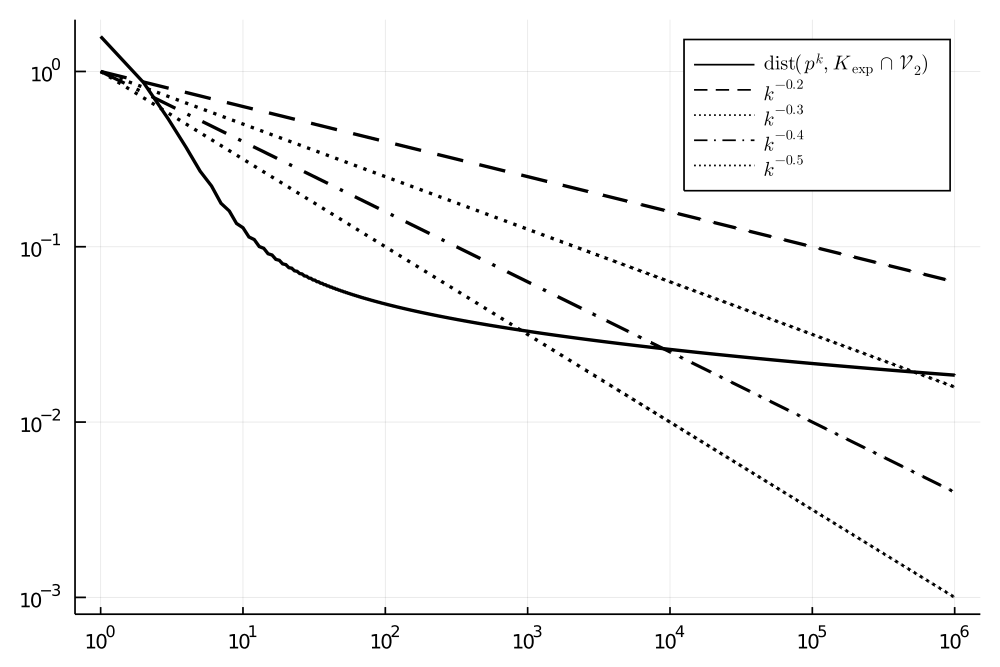
Next, we move on to (6.7). By item $(iv)$ of Proposition 6.9, we have that the convergence rate is at least logarithmic. In principle, this does not exclude the possibility that the true convergence rate of ${\rm dist}(p^{k},K_{\exp}\cap\mathcal{V}_{2})$ is faster. However, Figure 2 suggests that ${\rm dist}(p^{k},K_{\exp}\cap\mathcal{V}_{2})$ goes to $0$ slower than $k^{-r}$ for any $r>0$ , which again suggests that $({(\Phi_{\ln})}_{\kappa}^{\spadesuit})^{-1}(-s)$ is reflective of the true convergence rate.

Refer to caption — Figure 2: Log-log plot of ${\rm dist}(p^{k},K_{\exp}\cap\mathcal{V}_{2})$ for the iterates generated by CPA. Starting point is $(1,1,1)$ . Dashed and dotted lines correspond to $k^{-r}$ for a few values of $r$ .

Remark 6.10 (On the exponential cone and beyond).

The exponential cone is a building block for modelling many important problems related to entropy optimization, geometric programming and others, see [19, 18, 47]. For example, the Kullback-Leibler divergence between two nonnegative vectors $x,y\in{\rm I\!R}^{n}$ is defined as $D(x,y)\coloneqq\sum_{i}x_{i}\ln(x_{i}/y_{i})$ and its epigraph is often modelled using $n$ exponential cones as follows:

t\geq t_{1}+\cdots+t_{n},\quad(-t_{i},x_{i},y_{i})\in K_{\exp},i\in{1,\ldots,n},

as indicated, for example, in [18, Section 1.1] and [47, Chapter 5]. In particular, the problem of minimizing the Kullback-Leibler divergence subject to linear constraints on $x$ and $y$ can be expressed as a conic linear program (CLP) over a product of exponential cones. Notably, in [45], the authors found that nearly one third of a library of more than $300$ instances of mixed integer continuous optimization problems can be modelled using mixed integer conic formulations with exponential cone constraints, see Table 1 therein. Certain relaxations of these problems naturally lead to CLPs over a direct product of exponential cones. Although we have discussed only the case of a single exponential cone, our results are representative of what can happen in more general settings.

There is now a larger movement towards algorithms, software and theory for non-symmetric cones with quite a few solvers supporting exponential cones, e.g., [35, 52, 20, 47]. These references also discuss other convex sets involving logarithms and exponentials, such as the the log-determinant cone in [20]. On a more speculative note, it seems likely that some intersections involving those sets will have non-Hölderian error bounds due to the presence of exponentials and logarithms. Therefore, the techniques discussed in this section and in Section 5 will likely be applicable as well.

7 Concluding remarks

In this paper we proposed the notion of (strict) consistent error bounds. Under a strict consistent error bound, we established convergence rates for a family of algorithms for the convex feasibility problem (CFP). The key idea is to construct an inverse smoothing function based on the corresponding consistent error bound function. Our analysis recovers several old results and also gives several new ones. We also apply the convergence results to conic feasibility problems in order furnish further links between the singularity degree of the underlying problem and the convergence rate of several algorithms. Another novel aspect is the usage of regularly varying functions, which allows to draw conclusions about convergence rates while avoiding certain complicated computations. To conclude this paper, we first make some comparisons to approaches based on the KL-property.

7.1 On the Kurdyka-Łojasiewicz (KL) property and related concepts

The Kurdyka-Łojasiewicz (KL) property is an important and remarkable tool for convergence analysis used successfully in several works [3, 4, 39], so in this subsection we make a few comparisons in order to explain what could or what could (probably) not be done under the KL framework.

First, there is a close relation between error bounds and the KL property in the presence of convexity. As shown in [12, Theorem 30] and [13, Theorem 5], under certain conditions on $\varphi$ , an error bound of the form “ ${\rm dist}(x,\,\mathop{\rm arg\,min}\,f)\leq\varphi(f(x))$ ” implies that $f$ satisfies the KL property with a desingularization function involving $\varphi$ . Under our setting, there are several candidates for $f$ but they will, in all likelihood, be functions involving terms of the form $\max_{i}{\rm dist}(x,\,C_{i})$ or positive combinations of the ${\rm dist}(x,C_{i})^{2}$ , for example.

The choice of $f$ must be typically tailored to the target algorithm. Our understanding is that most of the algorithms in Section 4.3 would require different choices of $f$ in order for the analysis to be carried out under the KL framework. Finding the appropriate $f$ can be nontrivial, as illustrated by the merit function for the Douglas-Rachdford algorithm in [38]. It might also be impossible in some cases. For example, based on a result by Baillon, Combettes and Cominetti [5], it is claimed in a footnote in [13] that there is no potential function corresponding to the cyclic projection algorithm (CPA, see Example 4.10) for more than two sets.

Once the appropriate potential function is identified, it is necessary to show that certain conditions hold for the potential function along the sequence, e.g., the sufficient decrease condition and the relative error condition, see [3, 4, 50]. These properties and Assumption 4.5 have a similar motivation: ensuring that the sequence generated by the underlying algorithm satisfies some desirable properties.

If a convergence rate is desired, one usually has to show that the potential function satisfies the KL property with some KL exponent. The general KL property holds under relatively mild conditions, but identifying the exponent (if one exists) is a more challenging task, see [39]. Due to [13, Theorem 5], existence of a KL exponent is equivalent to the validity of a Hölderian error bound, so establishing the former or the latter are tasks of comparable difficulty. We note that the logarithmic error bound example in (6.7) can be used to construct a function which does not have a KL exponent, see [40, Example 4.22]. Similarly, $f_{\gamma}$ in Example 5.9 has no KL exponent. In particular, the convergence rate results based on the existence of a KL exponent do not seem applicable to (6.7) nor to Example 5.9.

That said, it is possible to analyze convergence rates without assuming that a KL exponent holds, see [12, Theorem 24] and [13, Theorem 14] for results which only rely on the desingularizing function $\varphi$ without assumptions on the format of $\varphi$ . And, interestingly, the existence of $\varphi$ can, sometimes, be characterized via certain integrals involving subgradient curves, see [12, Theorem 18]. However, we do not immediately see a connection between the integrals appearing in [12, Theorem 18] and in (4.3). We do note, however, that a certain optimal desingularizing function can be characterized via an integral, see [58, Section 3.2]. Similarly, if the best consistent error bound function in Proposition 3.3 is strict, it can be used to construct the inverse smoothing function $\Phi_{\kappa}^{\spadesuit}$ as in (4.3). So both integrals seem to be able to capture optimal phenomena, under certain conditions.

Another point is that the upper bounds in [12, Theorem 24] and [13, Theorem 14] include expressions of the format $\varphi(f(x^{k})-\kappa)$ (for some constant $\kappa$ ), so they are still dependent on the iterate $x^{k}$ and it might be fair to say they require some work in order to get an explicit convergence rate in terms of $k$ . In contrast, our upper bound on the convergence rate in (4.10) does not rely on the iterate $x^{k}$ and only uses the iteration number $k$ itself, which gives a more explicit expression. The drawback is that one must deal with the $(\Phi_{\widehat{\kappa}}^{\spadesuit})^{-1}$ term that appears in (4.10), which is indeed nontrival. Nevertheless, as shown in Section 5 and illustrated in Section 6.2, there are ways of bypassing this difficulty if the consistent error bound function is a function of regular variation.

Finally, we remark that the KL inequality is, of course, heavily connected to semialgebraic geometry [11], so one might wonder the extent to which our results could also be obtained by imposing semialgebraic assumptions on $\Phi$ or on the sets $C_{i}$ . Our assessment is that this seems unlikely, because the results in Section 5 are also applicable to sets and functions involving exponentials and logarithms (as in Example 5.9 and Section 6.2), which are not semialgebraic in general.

7.2 Future directions

At last, we mention some possible future directions. In the concluding remarks of [14], the authors mention the characterization of convergence rates in the absence of Hölderian regularity as an area of future research. We believe that the tools developed in this paper are a step forward towards this research goal, since Theorem 4.7 is quite general. And, indeed, we were able to reason about convergence rates in non-Hölderian settings as described in Sections 5.1 and 6.2.

In addition, it might be fair to say that regular variation has been rarely explored in the context of optimization algorithms and we believe there is significant room for further exploration. For example, we showed that consistent error bound functions always exist (Proposition 3.3). It could be interesting to try to prove whether a regularly varying consistent error bound function always exists as well. Since regular variation is connected to upper bounds for the convergence rate (Theorem 5.7), exploring this kind of question might lead to some insights on whether arbitrary slow convergence is possible in finite dimensions, which is another open problem mentioned in the conclusion of [14].

Finally, we believe it would be interesting to analyse convergence rates of other algorithms beyond projection methods. A natural candidate would be the Douglas-Rachford (DR) algorithm [25, 41], which was also extensively analyzed in [14]. However, the convergence rate results obtained in [14, Proposition 4.2] require not only an error bound condition on the underlying sets, but also a semialgebraic assumption. This suggests that it might be hard to obtain convergence rates for the DR algorithm purely based on consistent error bounds. On the other hand, damped versions of the DR algorithm (see [14, Section 5] or [23, Equation (25)]) might be more amenable to our techniques. In fact, sublinear rates were proved in [14, Theorem 5.2] when the underlying error bound is Hölderian without the need of imposing extra assumptions, see also [14, Remark 5.3]. In view of this, we believe it is likely that a result analogous to Theorem 4.7 and suitable for damped DR algorithms holds.

Acknowledgements

We thank the referees and the associate editor for their comments, which helped to improve the paper. The authors would like to thank Masaru Ito and Ting Kei Pong for the feedback and helpful comments during the writing of this paper. The first author is supported by ACT-X, Japan Science and Technology Agency (Grant No. JPMJAX210Q). The second author is partially supported by the JSPS Grant-in-Aid for Young Scientists 19K20217 and the Grant-in-Aid for Scientific Research (B)18H03206 and 21H03398.

Appendix A Proof of Lemma 4.2

Proof.

The fact that $f^{-}(0)=0$ follows from $f(0)=0$ and the definition (4.2). We also note that in (4.2), if we increase $s$ , the set after the ‘ ${\rm inf}$ ’ potentially shrinks, so $f^{-}$ is monotone nondecreasing. Next, we prove each item.

$(i)$

Fix any $s\in(0,\,\sup f)$ . Suppose that $f^{-}(s)=0$ . By the definition (4.2), given any $\epsilon_{k}>0$ , there exists $t_{k}\in[0,\,\epsilon_{k}]$ such that $f(t_{k})\geq s$ . Consequently, there exists a sequence $t_{k}\to 0_{+}$ with $f(t_{k})\geq s>0$ . This together with $f(0)=0$ contradicts the (right)-continuity of $f$ at $0$ , and thus proves $(i)$ .
$(ii)$

Let $s\geq 0,t\geq 0$ be such that $s\leq f(t)$ . Since $f$ is monotone increasing, $\sup f$ is never attained, which implies $0\leq s\leq f(t)<\sup f$ . Furthermore, by the definition (4.2), we have $f^{-}(s)\leq t$ .
$(iii)$

Let $s\geq 0,t\geq 0$ be such that $s<\sup f$ and $f(t)<s$ . By definition, $f^{-}(f(t)):={\rm inf}\left\{u\geq 0:f(u)\geq f(t)\right\}$ , therefore $f^{-}(f(t))\leq t$ . On the other hand, the strict monotonicity of $f$ implies that there is no $u<t$ with $f(u)\geq f(t)$ . This implies $f^{-}(f(t))\geq t$ and thus $f^{-}(f(t))=t$ . Together with the monotonicity of $f^{-}$ , we obtain $t=f^{-}(f(t))\leq f^{-}(s)$ .
$(iv)$

Suppose that there exists some $\widebar{s}\in(0,\,\sup f)$ such that $f^{-}$ is not continuous at $\widebar{s}$ . Since $f^{-}$ is monotone, both the left-sided limit $f^{-}(\widebar{s}-)$ and the right-sided limit $f^{-}(\widebar{s}+)$ exist and $f^{-}(\widebar{s}-)<f^{-}(\widebar{s}+)$ . Fix any $t\in(f^{-}(\widebar{s}-),\,f^{-}(\widebar{s}+))$ . From the monotonicity of $f^{-}$ , there exists $\epsilon>0$ such that whenever $s_{1},s_{2}$ satisfy $0<s_{1}<\widebar{s}<s_{2}<\sup f$ we have

$f^{-}(s_{1})<t-\epsilon<t+\epsilon<f^{-}(s_{2}).$

We now show that $f(t)=\widebar{s}$ . Suppose that $f(t)\neq\widebar{s}$ . Then either $f(t)<\widebar{s}$ or $f(t)>\widebar{s}$ . If $f(t)<\widebar{s}$ , let $s_{1}=(f(t)+\widebar{s})/2\in(f(t),\,\widebar{s})$ . Thus, we know from item $(iii)$ that $f^{-}(s_{1})\geq t$ , which contradicts $f^{-}(s_{1})<t-\epsilon$ .

If $f(t)>\widebar{s}$ , let $s_{2}=(f(t)+\widebar{s})/2\in(\widebar{s},\,f(t))$ . Then, from item $(ii)$ , we have $f^{-}(s_{2})\leq t$ , which contradicts $t+\epsilon<f^{-}(s_{2})$ . This proves $f(t)=\widebar{s}$ . The arbitrariness of $t\in(f^{-}(\widebar{s}-),\,f^{-}(\widebar{s}+))$ contradicts the strict monotonicity of $f$ . Consequently, $f^{-}$ is continuous on $(0,\,\sup f)$ .

∎∎

References

[1] S. Agmon. The relaxation method for linear inequalities. Canadian Journal of Mathematics, 6:382–392, 1954.
[2] R. Aharoni and Y. Censor. Block-iterative projection methods for parallel computation of solutions to convex feasibility problems. Linear Algebra and its Applications, 120:165 – 175, 1989.
[3] H. Attouch, J. Bolte, P. Redont, and A. Soubeyran. Proximal alternating minimization and projection methods for nonconvex problems: an approach based on the Kurdyka-Łojasiewicz inequality. Mathematics of Operations Research, 35(2):438–457, 2010.
[4] H. Attouch, J. Bolte, and B. F. Svaiter. Convergence of descent methods for semi-algebraic and tame problems: proximal algorithms, forward–backward splitting, and regularized Gauss–Seidel methods. Mathematical Programming, 137(1-2):91–129, 2013.
[5] J.-B. Baillon, P. Combettes, and R. Cominetti. There is no variational characterization of the cycles in the method of periodic projections. Journal of Functional Analysis, 262(1):400 – 408, 2012.
[6] H. H. Bauschke and J. M. Borwein. On projection algorithms for solving convex feasibility problems. SIAM Review, 38(3):367–426, 1996.
[7] H. H. Bauschke, J. M. Borwein, and W. Li. Strong conical hull intersection property, bounded linear regularity, Jameson’s property (G), and error bounds in convex optimization. Mathematical Programming, 86(1):135–160, 1999.
[8] A. Beck and M. Teboulle. Convergence rate analysis and error bounds for projection algorithms in convex feasibility problems. Optimization Methods and Software, 18(4):377–394, 2003.
[9] N. H. Bingham, C. M. Goldie, and E. Omey. Regularly varying probability densities. Publications de l’Institut Mathématique. Nouvelle Série, 80:47–57, 2006.
[10] N. H. Bingham, C. M. Goldie, and J. L. Teugels. Regular Variation. Encyclopedia of Mathematics and its Applications. Cambridge University Press, 1987.
[11] J. Bochnak, M. Coste, and M.-F. Roy. Real Algebraic Geometry. Springer Science, 1998.
[12] J. Bolte, A. Daniilidis, O. Ley, and L. Mazet. Characterizations of Łojasiewicz inequalities: subgradient flows, talweg, convexity. Transactions of the American Mathematical Society, 362(6):3319–3363, 2010.
[13] J. Bolte, T. P. Nguyen, J. Peypouquet, and B. W. Suter. From error bounds to the complexity of first-order descent methods for convex functions. Mathematical Programming, 165(2):471–507, 2017.
[14] J. M. Borwein, G. Li, and M. K. Tam. Convergence rate analysis for averaged fixed point iterations in common fixed point problems. SIAM Journal on Optimization, 27(1):1–33, 2017.
[15] J. M. Borwein, G. Li, and L. Yao. Analysis of the convergence rate for the cyclic projection algorithm applied to basic semialgebraic convex sets. SIAM Journal on Optimization, 24(1):498–527, 2014.
[16] J. M. Borwein and H. Wolkowicz. Regularizing the abstract convex program. Journal of Mathematical Analysis and Applications, 83(2):495 – 530, 1981.
[17] Y. Censor. Row-action methods for huge and sparse systems and their applications. SIAM Review, 23(4):444–466, 1981.
[18] V. Chandrasekaran and P. Shah. Relative entropy optimization and its applications. Mathematical Programming, 161(1):1–32, 2017.
[19] R. Chares. Cones and interior-point algorithms for structured convex optimization involving powers and exponentials. Phd thesis, Université catholique de Louvain, 2009.
[20] C. Coey, L. Kapelevich, and J. P. Vielma. Solving natural conic formulations with Hypatia.jl. ArXiv e-prints, 2021. arXiv:2005.01136.
[21] P. L. Combettes. The convex feasibility problem in image recovery, volume 95, pages 155–270. Elsevier, 1996.
[22] P. L. Combettes. Hilbertian convex feasibility problem: Convergence of projection methods. Applied Mathematics and Optimization, 35(3):311–330, 1997.
[23] D. Davis and W. Yin. Faster convergence rates of relaxed Peaceman-Rachford and ADMM under regularity assumptions. Mathematics of Operations Research, 42(3):783–805, 2017.
[24] D. Djurčić and A. Torgašev. Some asymptotic relations for the generalized inverse. Journal of Mathematical Analysis and Applications, 335(2):1397–1402, 2007.
[25] J. Douglas and H. H. Rachford. On the numerical solution of heat conduction problems in two and three space variables. Transactions of the American Mathematical Society, 82(2):421–439, 1956.
[26] D. Drusvyatskiy, G. Li, and H. Wolkowicz. A note on alternating projections for ill-posed semidefinite feasibility problems. Mathematical Programming, 162(1):537–548, 2017.
[27] P. Embrechts and M. Hofert. A note on generalized inverses. Mathematical Methods of Operations Research, 77(3):423–432, 2013.
[28] J. Faraut and A. Korányi. Analysis on Symmetric Cones. Oxford Mathematical Monographs. Clarendon Press, Oxford, 1994.
[29] L. Faybusovich. Several Jordan-algebraic aspects of optimization. Optimization, 57(3):379–393, 2008.
[30] H. A. Friberg. Projection onto the exponential cone: a univariate root-finding problem. Optimization Online, Jan. 2021.
[31] P. Gilbert. Iterative methods for the three-dimensional reconstruction of an object from projections. Journal of Theoretical Biology, 36(1):105–117, 1972.
[32] D. Henrion and J. Malick. Projection methods for conic feasibility problems: applications to polynomial sum-of-squares decompositions. Optimization Methods and Software, 26(1):23–46, 2011.
[33] G. T. Herman, A. Lent, and P. H. Lutz. Relaxation methods for image reconstruction. Communications of the ACM, 21(2):152–158, 1978.
[34] M. Ito and B. F. Lourenço. A bound on the Carathéodory number. Linear Algebra and its Applications, 532:347 – 363, 2017.
[35] M. Karimi and L. Tunçel. Domain-Driven Solver (DDS) Version 2.0: a MATLAB-based software package for convex optimization problems in domain-driven form. ArXiv e-prints, 2019. arXiv:1908.03075.
[36] M. Koecher. The Minnesota Notes on Jordan Algebras and Their Applications. Number 1710 in Lecture Notes in Mathematics. Springer, Berlin, 1999.
[37] A. S. Lewis and J.-S. Pang. Error bounds for convex inequality systems. In J.-P. Crouzeix, J.-E. Martinez-Legaz, and M. Volle, editors, Generalized Convexity, Generalized Monotonicity: Recent Results, pages 75–110. Springer US, 1998.
[38] G. Li and T. K. Pong. Douglas-Rachford splitting for nonconvex optimization with application to nonconvex feasibility problems. Mathematical Programming, 159(1):371–401, 2016.
[39] G. Li and T. K. Pong. Calculus of the exponent of Kurdyka–Łojasiewicz inequality and its applications to linear convergence of first-order methods. Foundations of Computational Mathematics, 18(5):1199–1232, 2018.
[40] S. B. Lindstrom, B. F. Lourenço, and T. K. Pong. Error bounds, facial residual functions and applications to the exponential cone. ArXiv e-prints, 2020. arXiv:2010.16391.
[41] P. L. Lions and B. Mercier. Splitting algorithms for the sum of two nonlinear operators. SIAM Journal on Numerical Analysis, 16(6):964–979, 1979.
[42] J. D. Loera, J. Haddock, and D. Needell. A sampling Kaczmarz-Motzkin algorithm for linear feasibility. SIAM Journal on Scientific Computing, 39(5):S66–S87, 2017.
[43] B. F. Lourenço. Amenable cones: error bounds without constraint qualifications. Mathematical Programming, 186:1–48, 2021.
[44] B. F. Lourenço, M. Muramatsu, and T. Tsuchiya. Facial reduction and partial polyhedrality. SIAM Journal on Optimization, 28(3):2304–2326, 2018.
[45] M. Lubin, E. Yamangil, R. Bent, and J. P. Vielma. Extended formulations in mixed-integer convex programming. In Q. Louveaux and M. Skutella, editors, Integer Programming and Combinatorial Optimization, pages 102–113, 2016.
[46] Z. Luo and P. Tseng. Error bounds and convergence analysis of feasible descent methods: a general approach. Annals of Operations Research, 46(1):157–178, 1993.
[47] MOSEK ApS. MOSEK Modeling Cookbook Release 3.2.3, 2021. URL: https://docs.mosek.com/modeling-cookbook/index.html.
[48] T. S. Motzkin and I. J. Schoenberg. The relaxation method for linear inequalities. Canadian Journal of Mathematics, 6:393–404, 1954.
[49] I. Necoara, P. Richtárik, and A. Patrascu. Randomized projection methods for convex feasibility: conditioning and convergence rates. SIAM Journal on Optimization, 29(4):2814–2852, 2019.
[50] P. Ochs. Unifying abstract inexact convergence theorems and block coordinate variable metric ipiano. SIAM Journal on Optimization, 29(1):541–570, 2019.
[51] J.-S. Pang. Error bounds in mathematical programming. Mathematical Programming, 79(1):299–332, 1997.
[52] D. Papp and S. Yıldız. alfonso: Matlab package for nonsymmetric conic optimization. ArXiv e-prints, 2021. arXiv:2101.04274.
[53] G. Pataki. Strong duality in conic linear programming: facial reduction and extended duals. In Computational and Analytical Mathematics, volume 50, pages 613–634. Springer New York, 2013.
[54] R. T. Rockafellar. Convex Analysis. Princeton University Press, 1997.
[55] E. Seneta. Regularly Varying Functions. Lecture Notes in Mathematics. Springer Berlin Heidelberg, 1976.
[56] J. F. Sturm. Error bounds for linear matrix inequalities. SIAM Journal on Optimization, 10(4):1228–1248, 2000.
[57] H. Waki and M. Muramatsu. Facial reduction algorithms for conic optimization problems. Journal of Optimization Theory and Applications, 158(1):188–215, 2013.
[58] X. Wang and Z. Wang. The exact modulus of the generalized concave Kurdyka-Łojasiewicz property. Mathematics of Operations Research, 2022.
[59] D. C. Youla and H. Webb. Image restoration by the method of convex projections: Part 1-theory. IEEE Transactions on Medical Imaging, 1(2):81–94, 1982.

	$\displaystyle{\rm dist}(x,\,C)$	$\displaystyle\leq\Phi(d(x),\,\\|x\\|)$
		$\displaystyle=\rho(\\|x\\|)\max(d(x)^{\gamma({\\|x\\|})},\,d(x))$
		$\displaystyle\leq\rho(r)\max(d(x)^{\gamma({\\|x\\|})},\,d(x)),$

Convergence analysis under consistent error bounds

Abstract

1 Introduction

1.1 Our contributions

2 Notation

3 Consistent error bound functions

Definition 3.1 (Consistent error bound functions).

Remark 3.2.

Proposition 3.3 (The best consistent error bound function).

Proof.

3.1 Hölderian and Lipschitzian error bounds

Definition 3.4 (Hölderian error bound).

Theorem 3.5 (Characterization of Hölderian error bounds).

Proof.

Example 3.6.

4 Convergence analysis under consistent error bounds

4.1 Inverse smoothing function from strict consistent error bound function

Lemma 4.1.

Lemma 4.2 (Properties of the generalized inverse).

Proposition 4.3 (The properties of Φκ♠\Phi_{\kappa}^{\spadesuit}).

Proof.

Proposition 4.4 (Asymptotical properties of Φκ♠\Phi_{\kappa}^{\spadesuit}).

Proof.

4.2 Convergence analysis of sequences

Assumption 4.5.

Proposition 4.6.

Proof.

Theorem 4.7.

Proof.

Remark 4.8 (No dependency on δ\delta in (4.10)).

Corollary 4.9.

Proof.

4.3 Projection algorithms

Example 4.10.

Lemma 4.11 (Checking Assumption 4.5).

Proof.

Corollary 4.12 (Hölderian error bounds and sublinear rates for projection algorithms).

Proof.

Theorem 4.13 (Convergence of a few common methods).

Proof.

Remark 4.14.

5 Regular variation and comparison of convergence rates

Definition 5.1 (Regularly varying functions).

Lemma 5.2.

Proof.

Theorem 5.3.

Proof.

Remark 5.4 (On assumption (ii) of Theorem 5.3).

Lemma 5.5 (Potter bounds).

Lemma 5.6.

Theorem 5.7 (Bounds on (Φκ♠)−1(\Phi_{\kappa}^{\spadesuit})^{-1}).

Proof.

5.1 Logarithmic error bounds

Definition 5.8 (Logarithmic error bound).

Example 5.9 (Example of logarithmic error bound in arbitrary dimension).

Lemma 5.10.

Proof.

Lemma 5.11.

Proof.

Theorem 5.12 (Tight bounds to (Φκ♠)−1(\Phi_{\kappa}^{\spadesuit})^{-1}).

Proof.

6 Convergence rate results for conic feasibility problems

Definition 6.1 (Facial residual functions).

Theorem 6.2 (Error bound for amenable cones, Theorem 23 in [43]).

Proposition 6.3.

Proof.

Proposition 6.4 (Existence of facial residual functions satisfying right-continuity at 00).

Proof.

6.1 The case of symmetric cones

Theorem 6.5 (Theorem 37 and Remark 39 of [43]).

Proposition 6.6.

Proof.

Theorem 6.7 (Convergence rate results for symmetric cones).

Proof.

Remark 6.8.

6.2 The exponential cone and non-Hölderian error bounds

Proposition 6.9.

Proof.

Remark 6.10 (On the exponential cone and beyond).

7 Concluding remarks

Proposition 4.3 (The properties of $\Phi_{\kappa}^{\spadesuit}$ ).

Proposition 4.4 (Asymptotical properties of $\Phi_{\kappa}^{\spadesuit}$ ).

Remark 4.8 (No dependency on $\delta$ in (4.10)).

Theorem 5.7 (Bounds on $(\Phi_{\kappa}^{\spadesuit})^{-1}$ ).

Theorem 5.12 (Tight bounds to $(\Phi_{\kappa}^{\spadesuit})^{-1}$ ).

Proposition 6.4 (Existence of facial residual functions satisfying right-continuity at $0$ ).