On the Robin spectrum for the hemisphereThanks: This research was supported by the European Research Council (ERC) under the European Union’s Horizon 2020 research and innovation programme (Grant agreement No. 786758) and by the Israel Science Foundation (grant No. 1881/20). We are grateful to Nadav Yesha for discussions on various aspects of this project.

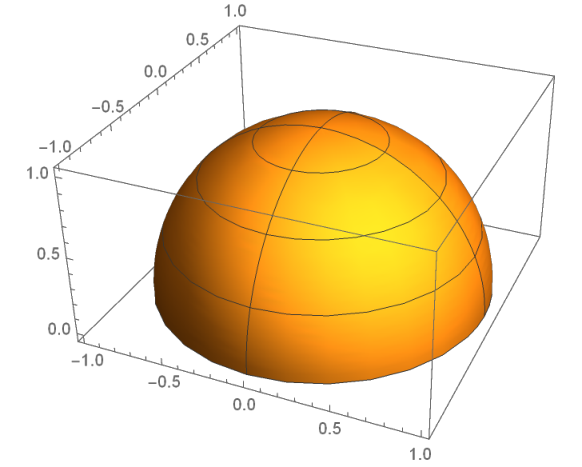
Let $\Omega$ be the upper unit hemisphere (Figure 1), with its boundary $\partial\Omega$ the equator. Our goal is to study the Robin boundary problem on the hemisphere $\Omega$:

where $\partial/\partial n$ is the derivative in the direction of the outward pointing normal to the equator, and $\sigma\geq 0$ is a constant.

The cases of Neumann and Dirichlet boundary conditions ($\sigma=0$ or $\sigma=\infty$) are classical [2, p. 243-244]: The eigenfunctions are restrictions to $\Omega$ of the eigenfunctions on the sphere (spherical harmonics), determined by the parity under reflection in the equator: The odd spherical harmonics give the Dirichlet eigenfunctions, the even ones give the Neumann eigenfunctions. The eigenvalues are thus of the form $\ell(\ell+1)$, where $\ell\geq 0$ is an integer, repeated with multiplicity $\ell+1$ for the Neumann case, and $\ell$ for the Dirichlet case.

The Robin spectrum is significantly less understood, and it is the main object of our interest. The problem admits separation of variables, and there is a basis of eigenfunctions in the form $f_{\nu,m}\linebreak=e^{im\phi}{\mathrm{P}}_{\nu}^{m}(\cos\theta)$, $m\in{\mathbb{Z}}$, where ${\mathrm{P}}_{\nu}^{m}(x)$ is an associated Legendre function. For each $m$, the admissible $\nu$’s are determined by the boundary condition.

Both $f_{\nu,m}$ and $f_{\nu,-m}$ share the same Laplace eigenvalue $\nu(\nu+1)$. Therefore the Robin spectrum admits a systematic double multiplicity, and we remove it beforehand by insisting that $m\geq 0$, resulting in a “desymmetrized spectrum”. Let $\lambda_{n}(0)$ denote the ordered desymmetrized Neumann eigenvalues (repeated with appropriate multiplicity), and for $\sigma>0$ we denote by $\lambda_{n}(\sigma)$ the ordered desymmetrized Robin eigenvalues, and define the Robin-Neumann (RN) gaps by

These were recently investigated in [9] in the case of planar domains, and will be the main object of study here.

We show that the desymmetrized Robin spectrum breaks up into small clusters $\mathcal{E}_{\ell}(\sigma)$ of size $\lfloor\ell/2\rfloor+1$, concentrated around the Neumann eigenvalues $\ell(\ell+1)$: For each eigenvalue $\nu(\nu+1)$, there is some $m\geq 0$, and a corresponding eigenfunction $e^{im\phi}{\mathrm{P}}_{\nu}^{m}(\cos\theta)$, so that the “degree” $\nu$ satisfies a secular equation $S_{m}(\nu)=\sigma$ , where

For any integer $\ell\geq m$ of the same parity ($\ell=m\bmod 2$), there is a unique solution $\nu_{\ell,m}(\sigma)$ in the open interval $(\ell,\ell+1)$. Denote by $\Lambda_{\ell,m}(\sigma)=\nu_{\ell,m}(\sigma)(\nu_{\ell,m}(\sigma)+1)$ the resulting Laplace eigenvalue. Then the desymmetrized spectrum consists of $\Lambda_{\ell,m}(\sigma)$, with $0\leq m\leq\ell$, and $m=\ell\bmod 2$, and is partitioned into disjoint clusters of size $\lfloor\ell/2\rfloor+1$:

We denote by $d_{\ell,m}(\sigma)$ the Robin-Neumann (RN) gaps in each cluster:

We have an asymptotic formula:

We display a plot of these RN gaps in Figure 2.

We show, using (1.1), that the RN gaps from each cluster have a limiting distribution, supported on the ray $[4\sigma/\pi,\infty)$:

Similarly, we can compute the mean value of the RN gaps within each cluster (§ 5.3):

Note that $2=2\operatorname{length}(\partial\Omega)/\operatorname{area}(\Omega)$, and the general theory¹¹ 1 Strictly speaking, the results of [9] are only for planar domains. developed in [9] leads to (1.2) if we average over the entire spectrum. Finer than that, (1.2) asserts that for the hemisphere the same mean result holds in each cluster.

The cluster structure that we find is similar in nature to that found for the spectrum of operator $-\Delta+V$ on the unit sphere²² 2 Similar results are available for the spectrum of the Laplace Beltrami operator on Zoll surfaces, which are spheres equipped with a Riemannian metric such that every geodesic is closed, and all geodesics have the same length. $S^{2}$, for a smooth potential $V$ [11, 12]. The eigenvalues of $-\Delta+V$ fall into clusters $C_{\ell}$ of diameter $O(1)$ around the eigenvalues $\ell(\ell+1)$ of the sphere (in our case, the clusters are bigger, of diameter $\approx\sqrt{\ell}$), and moreover the eigenvalues in each cluster $C_{\ell}$ become equidistributed with respect to a suitable measure.

We next examine the totality of the Robin-Neumann gaps $d_{n}(\sigma):=\lambda_{n}(\sigma)-\lambda_{n}(0)$.

In particular the Robin-Neumann gaps for the hemisphere are unbounded. We note that at this point, we do not know of any planar domain where the RN gaps are provably unbounded [9]. The upper bound is better than what is known for general smooth planar domains [9], which is $d_{n}(\sigma)\leq C\lambda_{n}(0)^{1/3}\cdot\sigma$.

As a corollary to Theorem 1.3 we establish the limit level spacing distribution for the Robin spectrum, which is the distribution $P(s)$ (assuming it exists) of the nearest-neighbour gaps $\lambda_{n+1}(\sigma)-\lambda_{n}(\sigma)$, normalized to have mean unity (cf § 7). In the case of the Neumann spectrum on the hemisphere, most of the nearest neighbour gaps $\lambda_{n+1}(0)-\lambda_{n}(0)$ are zero and $P(s)$ is the delta function at the origin. We show that the Robin spectrum has the same level spacing distribution;

However, unlike in the Neumann or Dirichlet case, the delta function is not a result of multiplicities, as there are none here:

We note that there are few deterministic simplicity results available, unlike generic simplicity which is more common, e.g. the Dirichlet spectrum of generic triangles is simple [5]. For instance, simplicity of the desymmetrized Dirichlet spectrum on the disk was proved by Siegel in 1929 (Bourget’s hypothesis) [10], and the same result holds for the Neumann spectrum [1]. However, there are arbitrarily small $\sigma>0$ for which the Robin spectrum on the disk has multiplicities [13]. For the square, we have a result analogous to Theorem 1.5 for $\sigma$ sufficiently small, but for rectangles with irrational squared aspect ratio, it fails for arbitrarily small $\sigma$ [8].

Finally, we note that the theory developed here for the hemisphere is quite singular when compared to what we expect to hold for all other spherical caps. In that case we do not expect a cluster structure and moreover, we believe that the level spacing distribution will be Poissonian ($P(s)=\exp(-s)$), as is expected for most integrable systems [3, 7], compare Figure 5.

Denote by $\Omega$ the upper hemisphere on the unit sphere, given in spherical coordinates as

so that the north pole is at $\theta=0$, and the equator, which is the boundary $\partial\Omega$, is at $\theta=\pi/2$.

We consider the Robin boundary problem on the hemisphere $\Omega$:

with $\nu>0$, where $\partial/\partial n$ is the derivative in the direction of the outward pointing normal to the equator, and $\sigma>0$. We will call $\nu$ the “degree”, in keeping with the case of Dirichlet or Neumann boundary conditions, when the eigenfunctions are spherical harmonics of degree $\ell$, with eigenvalue $\ell(\ell+1)$.

For $\sigma>0$, all eigenvalues $\lambda=\nu(\nu+1)$ are positive, hence $\nu$ is real and $\nu>0$ or $\nu<-1$. Since the two solutions of $\lambda=\nu(\nu+1)$ are $\nu$ and $-1-\nu$, we may assume that $\nu>0$.

The Laplacian commutes with rotations, hence the problem admits a separation of variables, according to symmetry under rotations $\{R_{\phi}\}$ around the north-south pole, which defines “sectors” consisting of functions transforming as $F(R_{\phi}x)=e^{im\phi}F(x)$ (here $m\in{\mathbb{Z}})$. We write such a Robin eigenfunction as

where $f(x)$ is a solution of ($x:=\cos\theta$)

The Robin boundary condition $\sigma F+\frac{\partial F}{\partial n}=0$ is then translated to

Indeed, the equator is $\theta=\pi/2$, or $x=0$; and the normal derivative (outward normal) is

Since the equation (2.1) is independent of the sign of $m$, we see that the Robin spectrum has a systematic double multiplicity. We will remove it (desymmetrization) by insisting that $m\geq 0$. Note that this is equivalent to taking only eigenfunctions which are symmetric with respect to the reflection $(x,y,z)\mapsto(x,-y,z)$. We order the desymmetrized Neumann eigenvalues (including multiplicities) by

The solutions of the differential equation (2.1) which are nonsingular in $0\leq x\leq 1$ form a one-dimensional space, all multiples of the associated Legendre functions (Ferrers functions) of the first kind ${\mathrm{P}}_{\nu}^{m}$ [6, 14.3.4]

Here ${\mathrm{F}}\left(a,b;c;z\right)$ is Olver’s hypergeometric series

with $(a)_{s}=\Gamma(a+s)/\Gamma(a)$, so that (2.3) converges absolutely if $x\in(-1,1]$, in particular in the range $x=\cos\theta\in[0,1]$ which is relevant for the hemisphere.

Denote the cluster (a multiset) of desymmetrized multiple Neumann eigenvalues sharing a common value of $\ell(\ell+1)$ by

This cluster has size $\#\mathcal{E}_{\ell}(0)=\lfloor\ell/2\rfloor+1$. We label the eigenvalues there by

where $L=L_{\ell}$ is given by

The distance of the Neumann eigenvalue cluster $\mathcal{E}_{\ell}(0)$ to the closest other Neumann eigenvalue cluster, which for $\ell\geq 1$ is $\mathcal{E}_{\ell-1}(0)$ (in other words, the distance between distinct nearby Neumann eigenvalues), is

We saw that the Robin eigenvalues are $\nu(\nu+1)$ where $\nu=\nu_{\ell,m}(\sigma)\in(\ell,\ell+1)$, $\ell=m\bmod 2$, is a solution of the secular equation $S_{m}(\nu)=\sigma$. Denote by

which is the evolution of the Neumann eigenvalue cluster $\mathcal{E}_{\ell}(0)$. Since $\ell<\nu_{\ell,m}(\sigma)<\ell+1$, the spectral cluster $\mathcal{E}_{\ell}(\sigma)$ is contained in the open interval $\Big(\ell(\ell+1),(\ell+1)(\ell+2)\Big)$, and in particular the evolved eigenvalue clusters $\mathcal{E}_{\ell}(\sigma)$ do not mix with each other.

Recall that we write $\nu_{\ell,m}(\sigma)=\ell+\delta_{\ell,m}(\sigma)$.

References

• [1] M. Ashu, Some properties of Bessel functions with applications to Neumann eigenvalues in the unit disc, Bachelor’s thesis 2013:K1 (E. Wahlén advisor), Lund University. http://lup.lub.lu.se/student-papers/record/7370
• [2] P. Bérard and G. Besson. Spectres et groupes cristallographiques. II. Domaines sphériques. Ann. Inst. Fourier (Grenoble) 30 (1980), no. 3, 237–248.
• [3] M.V.Berry and M. Tabor. Level clustering in the regular spectrum. Proc. R. Soc. London A356, 375–394 (1977).
• [4] G. V. Haines. Spherical cap harmonic analysis. J. Geophys. Res. 90 (B3): 2583–2591.
• [5] L. Hillairet and C. Judge. Spectral simplicity and asymptotic separation of variables. Comm. Math. Phys. 302 (2011), no. 2, 291–344. Erratum: Comm. Math. Phys. 311 (2012), no. 3, 839–842.
• [6] NIST Digital Library of Mathematical Functions (DLMF). Available online at https://dlmf.nist.gov/
• [7] Z. Rudnick. What is… quantum chaos? Notices Amer. Math. Soc. 55 (2008), no. 1, 32–34.
• [8] Z. Rudnick and I. Wigman, in preparation.
• [9] Z. Rudnick, I. Wigman and N. Yesha. Differences between Robin and Neumann eigenvalues, available online https://arxiv.org/abs/2008.07400.
• [10] C. L. Siegel, Über einige Anwendungen diophantischer Approximationen, Abh. Preuss. Akad. Wiss., Phys.-math. Kl., (1929).
• [11] A. Weinstein. Asymptotics of eigenvalue clusters for the Laplacian plus a potential. Duke Math. J. 44 (1977), no. 4, 883–892.
• [12] H. Widom. Eigenvalue distribution theorems for certain homogeneous spaces. J. Functional Analysis 32 (1979), no. 2, 139–147.
• [13] N. Yesha, private communication.