Selecting Energy Efficient Inputs using Graph Structure

Graphs are denoted $\mathcal{G}=(\mathcal{V},\mathcal{E})$ which consist of $|\mathcal{V}|=n$ nodes and edges $(v_{j},v_{k})\in\mathcal{E}$ which may be read ‘from node $v_{j}$ to node $v_{k}$.’ Unless otherwise stated, all graphs considered here are assumed to be directed. The set of neighbors of a node $v_{j}$, denoted $\mathcal{N}_{j}$, is defined as the set of nodes $v_{k}$ such that $(v_{k},v_{j})\in\mathcal{E}$. We do not include any loops, that is an edge $(v_{j},v_{j})$, in the set of edges, as loops are treated separately. A graph may be represented as an adjacency matrix, $A\in\mathbb{R}^{n\times n}$, which has elements $A_{j,k}>0$ if $(v_{k},v_{j})\in\mathcal{E}$ and $A_{j,k}=0$ otherwise. The diagonal of the matrix $A$, $A_{j,j}<0$, $j=1,\ldots,n$, represent the loops present at each node. In this paper, we assume uniform edge weights and uniform loop weights, that is, edge weights are equal, $A_{j,k}=A_{j^{\prime},k^{\prime}}$ for all $(v_{j},v_{k}),(v_{j^{\prime}},v_{k^{\prime}})\in\mathcal{E}$ and $(v_{j^{\prime}},v_{k^{\prime}})\in\mathcal{E}$ and all loop weights are equal, $A_{j,j}=A_{k,k}$, for all $j,k=1,\ldots,n$. The edge weight is denoted $\gamma>0$ and the loop weight is denoted $-\nu<0$.

A permutation of a set of $n$ elements, $\pi$, can also be expressed as a matrix, $P\in\{0,1\}^{n\times n}$, with elements $P_{j,k}=1$ if $\pi(v_{j})=v_{k}$ and $P_{j,k}=0$ otherwise. Applying the permutation to the adjacency matrix yields the permuted adjacency matrix $A^{\pi}=PAP^{T}$. If $\pi$ is a symmetry then $A^{\pi}=A$ (assuming uniform edge weights and loop weights as specified above).
The orbit indicator matrix, $E\in\{0,1\}^{n\times q}$, has elements $E_{j,k}=1$ if node $v_{j}\in\mathcal{O}_{k}$ and $E_{j,k}=0$ otherwise. The adjacency matrix of the quotient graph, $A^{Q}\in\mathbb{R}^{q\times q}$, can be found by applying the orbit indicator matrix,

where the superscript $\dagger$ denotes the Moore-Penrose pseudoinverse, defined as $E^{\dagger}=(E^{T}E)^{-1}E^{T}$. The elements of the quotient graph adjacency matrix, $A_{j,k}^{Q}$, are equal to the number of neighbors of a node $v_{\ell}\in\mathcal{O}_{j}$ that are in $\mathcal{O}_{k}$ (multiplied by the uniform edge weight $\gamma$).

Each node is assigned a time-varying state, denoted $x_{j}(t)$, $j=1,2,\ldots,n$, whose behavior is governed by its neighbors. We are able to influence the dynamics through a subset of the nodes, $\mathcal{D}\subseteq\mathcal{V}$, defined as the $|\mathcal{D}|=m$ driver nodes. The driver node set can be represented as a matrix, $B\in\{0,1\}^{n\times m}$, where each column of $B$ has a single nonzero element corresponding to a driver node. An independent, external, control input, denoted $u_{\ell}(t)$, $\ell=1,\ldots,m$, is assigned to each driver node $v_{k}\in\mathcal{D}$. The states evolve in time according to a system of linear differential equations where the state matrix $A$ is the adjacency matrix of a graph.

An initial condition is assigned to each node at time $t=0$, $x_{j}(0)=x_{j,0}$. The set of $p$ target nodes, denoted $\mathcal{T}\subseteq\mathcal{V}$, are those whose states we would like to drive to a particular value at some final time $t=t_{f}$. The set of target nodes can also be represented as a matrix, $C\in\{0,1\}^{p\times n}$, where each row has a single nonzero element corresponding to a target node.

If the matrix $A$ is Hurwitz and $t_{f}$ is chosen large enough, then it may be appropriate to use $W$ instead of $W(t_{f})$.

The output controllability Gramian appears in the solution to the following optimal control problem.

Given matrices $A$, $B$, and $C$, from Lemma 2.5, the minimum energy optimal control problem can be solved for $\textbf{u}:[0,t_{f}]\mapsto\mathbb{R}^{m}$ with associated cost $J^{*}$. In this paper, we are interested instead in the scenario where $A$ and $C$ are provided but we may choose the set of driver nodes $\mathcal{D}\subseteq\mathcal{V}$ (equivalently the matrix $B$ with the restrictions described previously) such that we minimize the control energy subject to a cardinality constraint on the set of driver nodes. For a graph with $n$ nodes, there are $\binom{n}{m}$ potential sets of $m$ driver nodes so a brute force search for even a moderate sized network is impossible. In addition, the solution to the minimum energy output control problem depends on the choice of control maneuver. To be more general, instead of minimizing the optimal cost $J^{*}$ in Eq. (10) which depends on $\bm{\beta}$ directly, an energy metric that is independent of the particular control maneuver, $M(\mathcal{D})$, is defined such that our choice of driver nodes are good in some average over the possible choices of control maneuver.

It has previously been shown (Olshevsky (2014)) that minimizing energy metrics are at least NP-hard problems, so rather than attempting to derive an algorithm to find the optimal solution to Eq. (12), heuristics and approximation algorithms must be used to return ‘good’ solutions (better than could be expected to be found during an extensive random search). The two choices of energy metric, $M(\mathcal{D})$, investigated here are the control volume and the expectation of the control energy.
The set of all control maneuvers capable of being performed with $E$ units of energy forms a $p$-dimensional ellipsoid.

The volume of the ellipsoid in Eq. (13) is known to be related to the determinant of the matrix $\bar{W}(t_{f})$.

The logarithm is taken of the volume as the determinant of the controllability Gramian can fall below the accuracy of double precision floating points values (Sun & Motter (2013)). In (Summers et al. (2016)), the energy metric in Eq. (14) is shown to be a submodular set function. The submodular property of Eq. (14) has not been directly applied to the target control problem (only the subproblem when $p=n$). Nonetheless, when $p<n$, the submodularity of the log-volume holds (Summers et al. (2016)) so we may use a greedy algorithm which retains the same approximation guarantee. For the metric to be minimized, we use the following inverse volume function.

Decreasing $-\text{Vol}(\mathcal{D})$ means the set of reachable states, or control maneuvers, is larger.
The second energy metric, the expectation of the control energy over initial conditions, assumes that $\bm{y}_{f}=\bm{0}_{p}$ and $\bm{x}_{0}$ is a vector of $n$ independent random variables with mean zero and variance one so that $\mathbb{E}[\bm{x}_{0}\bm{x}_{0}^{T}]=I_{n}$. The covariance matrix of the control maneuver can be written (G. Li, Hu et al. (2016)),

The expectation of the control energy over the control maneuvers is the metric to be minimized.

The following sections describe heuristics to solve Eq. (12) when $M(\mathcal{D})=\text{Vol}(\mathcal{D})$ and when $M(\mathcal{D})=\bar{E}(\mathcal{D})$.

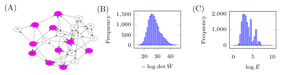
A directed graph is shown in Fig. 1(A) with $n=20$ nodes and $p=10$ target nodes highlighted in pink. The goal is to select $m=5$ driver nodes such that Eq. (12) is minimized for either of the two energy metrics considered. This problem is small enough so that a brute force search can be employed. In Figs. 1(B) and 1(C), all sets of five nodes are set as the driver node set successively and both energy metrics are computed. In both cases, the determinant of the output Gramian and the expectation of the control energy span multiple orders of magnitude so choosing an energy efficient set of driver nodes is important. In the following section, we present our heuristic method to find a set of driver nodes that is energy efficient which uses only structural properties of the graph.

A model that captures these two properties is the directed balloon graph that consists of two end nodes, labeled $0$ and $d$, and $b$ disjoint directed paths from node $0$ to node $d$ (I. Klickstein et al. (2018); I.S. Klickstein & Sorrentino (2018)). A single control input is attached to node $0$ while $d$ is the single target node. Each edge is assumed to have uniform weight $\gamma>0$ and each loop has uniform weight $-\nu<0$. The driver node $0$ and target node $d$ are separated by distance $d_{0,d}=d$ and, from the definition of redundancy in Eq. (18), $r_{0,d}=b$. The quotient graph of the balloon graph is a directed path graph with uniform edge weights $\gamma$ and loop weights $-\nu$ except for the last edge, $(d-1,d)$, which has edge weight $b\gamma$.
The output controllability Gramian when there is a single target node, say $\mathcal{T}=\{d\}$, is only the corresponding diagonal element $W_{d,d}(t)$. To determine the effect that distance and redundancy has on the control energy, this element of the controllability Gramian of the balloon graph’s quotient graph is derived analytically.

From Eq. (10), the minimum control energy for the balloon graph is $J^{*}\propto W_{d,d}^{-1}(t_{f})$, or if $t_{f}$ is large enough, then $J^{*}\propto W_{d,d}^{-1}$. Using Stirling’s approximation for the binomial coefficient, the control energy is approximately,

Our structure based metric that approximates the control energy uses this pair-wise energy cost. Given a set of $m$ driver nodes $\mathcal{D}$ and a set of $p$ target nodes $\mathcal{T}$, and pairwise distances $d_{j,k}$ and redundancies $r_{j,k}$ from each node to each target node, we can construct the pair-wise cost matrix $F\in\mathbb{R}^{n\times p}$ which has elements,

Each term, $F_{j,k}$ in Eq. (38) can be thought of as the cost of controlling the $k$’th target node with node $v_{j}$. The structure based metric then assigns target nodes to driver nodes by selecting which node $v_{j}\in\mathcal{D}$ can control the $k$’th target node the most cheaply (that is, $F_{j,k}$ is minimized over all other possible choices of driver node).

We propose that this structure based metric can be a surrogate function to replace Eq. (15) or Eq. (17) when trying to determine a set of driver nodes that minimizes one of the energy metrics. To test this proposal, we pick random sets of nodes from graphs using a hill climbing procedure to sample the full range of $\text{FLP}(\mathcal{D})$ and compute both $\text{FLP}(\mathcal{D})$ and $\text{Vol}(\mathcal{D})$ (or $\bar{E}(\mathcal{D})$).

The relationship between the ellipsoid volume cost in Eq. (15) and the FLP cost in Eq. (39) is shown for four example graphs in Fig. 3. Each graph has $n=300$ nodes, $p=100$ target nodes selected randomly, and a driver node set of $m=33$ nodes to be determined. The four graphs’ method of construction is described in the captions of Fig. 3. The log volume cost in Eq. (14) appears on the vertical axis of each plot while the FLP cost appears on the horizontal axis. From the trends in Fig. 3, it is clear that if we were to find a driver node set $\mathcal{D}$ that minimized $\text{FLP}(\mathcal{D})$, that set of driver nodes would also be a competitive solution for the original optimization problem minimizing $\text{Vol}(\mathcal{D})$.
The pair-wise cost in Eq. (39) is also shown to correlate with the expectation cost used by LPGM in Eq. (17). A demonstration of this relation is shown in Fig. 4 for four types of graphs described in the caption. The two costs, $\bar{E}(\mathcal{D})$ and $\text{FLP}(\mathcal{D})$ are positively correlated as shown by the linear fitted line in red. Again, any driver node set $\mathcal{D}$ that minimizes $\text{FLP}(\mathcal{D})$ would be a competitive solution for the $\bar{E}(\mathcal{D})$ minimization problem as well.
Next, we present a method based on the facility location problem (Mirchandani & Francis (1990)) to minimize $\text{FLP}(\mathcal{D})$ so that we may compare the obtained solutions with those generated by published heuristics to optimize Eq. (12) with either $M(\mathcal{D})=\text{Vol}(\mathcal{D})$ or $M(\mathcal{D})=\bar{E}(\mathcal{D})$.

Facility location problems (FLP) originally arose to address the problem of choosing distribution centers to accommodate demands while minimizing transportation costs (Mirchandani & Francis (1990)). Let there be $p$ locations that must be supplied from $m$ distribution centers selected from $n\geq m$ possible choices. The cost of supplying the $j$’th location from the $k$’th distribution center is denoted $c_{j,k}$. Each location is assumed to be supplied from a single distribution center. Let the binary variables $Y_{j}\in\{0,1\}$, $j=1,\ldots,n$, be the possible distribution centers where $Y_{j}=1$ if it is chosen to be a distribution center and $Y_{j}=0$ otherwise. Let the binary variables $Z_{j,k}\in\{0,1\}$, $j=1,\ldots,n$, $k=1,\ldots,p$, denote assignments so that if distribution center $j$ supplies location $k$ then $Z_{j,k}=1$ and $Z_{j,k}=0$ otherwise.
The FLP can be posed as an integer linear programming (ILP) with binary variables.

The first constraint ensures that precisely $m$ locations are chosen to be distribution centers. The second constraint ensures that each location to be supplied is assigned to a single distribution center. The third constraint ensures locations to be supplied are only assigned to distribution centers that are opened.
Even large instances ($n\approx 1000$) of the can be solved efficiently with ILP solvers such as the GNU Linear Programming Kit (Makhorin (2018)). For larger instances of Eq. (40), one can use recently developed specialized algorithms to approximately solve the FLP with an approximation guarantee (Jain et al. (2002)) efficiently.

A greedy algorithm that starts with an empty set and at each iteration adds the single node to the driver node set that improves the cost function the most has an approximation guarantee of $63\%$ when the cost function is submodular (Fisher et al. (1978)).
By the definition of the matrix $B$ we impose, the matrix product can be decomposed into the individual contributions of each driver node $BB^{T}=\sum_{k\in\mathcal{D}}\bm{e}_{k}\bm{e}_{k}^{T}$ where $\bm{e}_{k}$ is the unit vector with the single non-zero element corresponding to each driver node. This decomposition can be used to split the differential Lyapunov equation in Eq. (5) into the contribution of each driver node as well.

A greedy algorithm to minimize $\text{Vol}(\mathcal{D})$ over the powerset of the nodes could be applied directly assuming perfect arithmetic.
The difficulty of applying the greedy algorithm directly arises in two ways. The first difficulty is that storing all potential contributions of each driver node requires $np^{2}$ double precision variables which, if $p$ is large, could be prohibitive. The second difficulty is computing $\text{Vol}(\mathcal{D})$ for the first few driver node sets as the Gramian is known to have extremely small (below double precision accuracy) eigenvalues when the number of target nodes is large relative to the number of driver nodes (I. Klickstein et al. (2017)). A proposed method (Summers et al. (2016)) to handle the first few driver nodes replaces the evaluation of $\text{Vol}(\mathcal{D})$ with $-\text{rank}_{num}(\mathcal{D})$ where the function $\text{rank}_{num}(\cdot)$ computes the numerical rank of the output Gramian $\bar{W}_{\mathcal{D}}(t_{f})$ (Sun & Motter (2013)). This substitute is used until enough driver nodes have been added by the greedy algorithm to ensure the output controllability Gramian is of full numerical rank. Algorithm 1 in Appendix A.1 shows this modified version where a flag is used to perform the switch from computing the rank to the determinant.

To minimize the expected energy cost in Eq. (17), a continuous relaxation step is introduced so that the previous restrictions on $B$ are removed, that is, now $B\in\mathbb{R}^{n\times m}$. The main result in (L. Gao et al. (2018)) that allows a gradient descent method to be used is the derivative of Eq. (17) with respect to $B$.

With information about the gradient, a projected gradient method can be used such that at each iteration the next $B$ matrix moves in the steepest descent direction until a local minimum is found. A probabilistic projection is used, $\mathcal{P}:\mathbb{R}^{n\times m}\mapsto 2^{\mathcal{V}}$, that finds a set of nodes of cardinality $m$ from a dense matrix, which is the solution returned for the original optimization problem. Details of the algorithm can be found in Algorithm 2 in Appendix A.2.

A comparison of the performance of the FLP method and the LPGM heuristic for sets of four types of graphs is shown in Fig. 6. As in Fig. 5, bars in front of the gray background represent cases where the FLP algorithm returns more energy efficient driver node sets than the LPGM algorithm and vice versa for the bars with a white background. For the four types of graphs examined, we see that neither the FLP method nor the LPGM heuristic perform better than the other, with some slight bias towards one or the other depending on the graph. The benefit of the FLP method is that it scales to larger problems better than the LPGM heuristic and it does not suffer from the same overflow/underflow issues as discussed in Appendix B.

References

- Arianos et al. ((2009)) Arianos, S., Bompard, E., Carbone, A. & Xue, F. (2009). Power grid vulnerability: A complex network approach. Chaos: An Interdisciplinary Journal of Nonlinear Science 19 1 13119. https://aip.scitation.org/doi/abs/10.1063/1.3077229http://aip.scitation.org/doi/10.1063/1.3077229 doi:10.1063/1.3077229
- Barabási et al. ((2000)) Barabási, A-L., Albert, R. & Jeong, H. (2000). Scale-free characteristics of random networks: the topology of the world-wide web. Physica A: statistical mechanics and its applications 281 1-4 69–77. https://www.sciencedirect.com/science/article/pii/S0378437100000182 doi:10.1016/S0378-4371(00)00018-2
- Bartels & Stewart ((1972)) Bartels, R.H. & Stewart, G.W. (1972). Solution of the matrix equation AX + XB = C [F4]. Communications of the ACM 15 9 820–826. http://portal.acm.org/citation.cfm?doid=361573.361582 doi:10.1145/361573.361582
- Bateman ((1954)) Bateman, H. (1954). Tables of Integral Transforms Volume I (A. Erd{’e}lyi, Ed.). : McGraw-Hill Book Company, Inc.
- Bovet & Makse ((2019)) Bovet, A. & Makse, H.A. (2019). Influence of fake news in Twitter during the 2016 US presidential election. Nature Communications 10 1 7. http://www.nature.com/articles/s41467-018-07761-2 doi:10.1038/s41467-018-07761-2
- Commault et al. ((2017)) Commault, C., Van Der Woude, J. & Boukhobza, T. (2017). On the fixed controllable subspace in linear structured systems. Systems & Control Letters 102 42–47.
- Fisher et al. ((1978)) Fisher, M.L., Nemhauser, G.L., Wolsey, L.A., Fisher, M.L., Nemhauser, G.L. & Wolsey, L.A. (1978). An analysis of approximations for maximizing submodular set functions—II. In Polyhedral combinatorics ( 14, 265–294). : Springer. https://link.springer.com/chapter/10.1007{%}2FBFb0121195http://link.springer.com/10.1007/BF01588971https://link.springer.com/article/10.1007/BF01588971 doi:10.1007/BF01588971
- J. Gao et al. ((2014)) Gao, J., Liu, Y-Y., D’Souza, R.M. & Barabási, A-L. (2014). Target control of complex networks. Nature Communications 5 1 5415. http://www.nature.com/articles/ncomms6415 doi:10.1038/ncomms6415
- L. Gao et al. ((2018)) Gao, L., Zhao, G., Li, G., Deng, L. & Zeng, F. (2018). Towards the minimum-cost control of target nodes in directed networks with linear dynamics. Journal of the Franklin Institute 355 16 8141–8157. https://linkinghub.elsevier.com/retrieve/pii/S0016003218305441 doi:10.1016/j.jfranklin.2018.08.011
- Grinberg et al. ((2019)) Grinberg, N., Joseph, K., Friedland, L., Swire-Thompson, B. & Lazer, D. (2019). Fake news on Twitter during the 2016 U.S. presidential election. Science 363 6425 374–378. https://www.sciencemag.org/lookup/doi/10.1126/science.aau2706 doi:10.1126/science.aau2706
- Guo et al. ((2021)) Guo, J., Ji, Z. & Liu, Y. (2021). Sufficient conditions and limitations of equivalent partition in multiagent controllability. SCIENCE CHINA Information Sciences .
- Iudice et al. ((2019)) Iudice, F.L., Sorrentino, F. & Garofalo, F. (2019). On node controllability and observability in complex dynamical networks. IEEE Control Systems Letters 3 4 847–852.
- Jain et al. ((2002)) Jain, K., Mahdian, M. & Saberi, A. (2002). A new greedy approach for facility location problems. In Proceedings of the thiry-fourth annual acm symposium on theory of computing - stoc ’02 (p. 731). New York, New York, USA: ACM Press. http://portal.acm.org/citation.cfm?doid=509907.510012 doi:10.1145/509907.510012
- Ji et al. ((2020)) Ji, Z., Lin, H., Cao, S., Qi, Q. & Ma, H. (2020). The complexity in complete graphic characterizations of multiagent controllability. IEEE Transactions on Cybernetics 51 1 64–76.
- Kailath ((1980)) Kailath, T. (1980). Linear systems. : Prentice hall Englewood Cliffs, NJ.
- I. Klickstein et al. ((2018)) Klickstein, I., Kafle, I., Bartaula, S. & Sorrentino, F. (2018). Energy Scaling with Control Distance in Complex Networks. In 2018 ieee international symposium on circuits and systems (iscas) ( 1–5). : IEEE. https://ieeexplore.ieee.org/document/8351828/ doi:10.1109/ISCAS.2018.8351828
- I. Klickstein et al. ((2017)) Klickstein, I., Shirin, A. & Sorrentino, F. (20171). Energy scaling of targeted optimal control of complex networks. Nature Communications 8 15145. https://www.nature.com/articles/ncomms15145http://www.nature.com/doifinder/10.1038/ncomms15145 doi:10.1038/ncomms15145
- I. Klickstein et al. ((2017)) Klickstein, I., Shirin, A. & Sorrentino, F. (20172). Locally Optimal Control of Complex Networks. Physical Review Letters 119 26 268301. https://link.aps.org/doi/10.1103/PhysRevLett.119.268301 doi:10.1103/PhysRevLett.119.268301
- I. Klickstein & Sorrentino ((2018)) Klickstein, I. & Sorrentino, F. (2018). Control Energy of Lattice Graphs. In 2018 ieee conference on decision and control (cdc) ( 6132–6138). : IEEE. https://ieeexplore.ieee.org/document/8619267/ doi:10.1109/CDC.2018.8619267
- I.S. Klickstein & Sorrentino ((2018)) Klickstein, I.S. & Sorrentino, F. (2018). Control Distance and Energy Scaling of Complex Networks. IEEE Transactions on Network Science and Engineering . https://ieeexplore.ieee.org/document/8576564/ doi:10.1109/TNSE.2018.2887042
- Lauri & Scapellato ((2016)) Lauri, J. & Scapellato, R. (2016). Topics in Graph Automorphisms and Reconstruction. : Cambridge University Press.
- G. Li, Deng et al. ((2018)) Li, G., Deng, L., Xiao, G., Tang, P., Wen, C., Hu, W.Stanley, H.E. (2018). Enabling Controlling Complex Networks with Local Topological Information. Scientific reports 8 1 4593. https://www.nature.com/articles/s41598-018-22655-5 doi:10.1038/s41598-018-22655-5
- G. Li, Ding et al. ((2018)) Li, G., Ding, J., Wen, C. & Huang, J. (2018). Minimum Cost Control of Directed Networks With Selectable Control Inputs. IEEE Transactions on Cybernetics 1–10. https://ieeexplore.ieee.org/document/8472257/ doi:10.1109/TCYB.2018.2868507
- G. Li, Ding et al. ((2016)) Li, G., Ding, J., Wen, C. & Pei, J. (2016). Optimal control of complex networks based on matrix differentiation. EPL (Europhysics Letters) 115 6 68005. http://stacks.iop.org/0295-5075/115/i=6/a=68005?key=crossref.f5c7966f46752ee3f06f968288acae99 doi:10.1209/0295-5075/115/68005
- G. Li, Hu et al. ((2016)) Li, G., Hu, W., Xiao, G., Deng, L., Tang, P., Pei, J. & Shi, L. (2016). Minimum-cost control of complex networks. New Journal of Physics 18 1 13012. http://iopscience.iop.org/article/10.1088/1367-2630/18/1/013012/meta doi:10.1088/1367-2630/18/1/013012
- Y.H. Li et al. ((2016)) Li, Y.H., Wang, P.P., Li, X.X., Yu, C.Y., Yang, H., Zhou, J.Zhu, F. (2016). The Human Kinome Targeted by FDA Approved Multi-Target Drugs and Combination Products: A Comparative Study from the Drug-Target Interaction Network Perspective. PLOS ONE 11 11 e0165737. https://dx.plos.org/10.1371/journal.pone.0165737 doi:10.1371/journal.pone.0165737
- Liu & Barabási ((2016)) Liu, Y-Y. & Barabási, A-L. (2016). Control principles of complex systems. Reviews of Modern Physics 88 3 35006. https://journals.aps.org/rmp/abstract/10.1103/RevModPhys.88.035006 doi:10.1103/RevModPhys.88.035006
- Liu et al. ((2011)) Liu, Y-Y., Slotine, J-J. & Barabási, A-L. (2011). Controllability of complex networks. Nature 473 7346 167–173. http://www.nature.com/doifinder/10.1038/nature10011 doi:10.1038/nature10011
- Lo Iudice et al. ((2015)) Lo Iudice, F., Garofalo, F. & Sorrentino, F. (2015). Structural permeability of complex networks to control signals. Nature Communications 6 1 8349. https://www.nature.com/articles/ncomms9349http://www.nature.com/articles/ncomms9349 doi:10.1038/ncomms9349
- Makhorin ((2018)) Makhorin, A. (2018). GNU Linear Programming Kit. Boston, MA: Free Software Foundation. https://www.gnu.org/software/glpk
- McKay & Piperno ((2014)) McKay, B.D. & Piperno, A. (2014). Practical graph isomorphism, II. Journal of Symbolic Computation 60 94–112. http://linkinghub.elsevier.com/retrieve/pii/S0747717113001193 doi:10.1016/j.jsc.2013.09.003
- Mirchandani & Francis ((1990)) Mirchandani, P.B. & Francis, R.L. (1990). Discrete location theory. : John Wiley & Sons, Inc.
- Olshevsky ((2014)) Olshevsky, A. (2014). Minimal controllability problems. IEEE Transactions on Control of Network Systems 1 3 249–258. https://ieeexplore.ieee.org/abstract/document/6851897/ doi:10.1109/TCNS.2014.2337974
- Pagani & Aiello ((2013)) Pagani, G.A. & Aiello, M. (2013). The power grid as a complex network: a survey. Physica A: Statistical Mechanics and its Applications 392 11 2688–2700. https://www.sciencedirect.com/science/article/pii/S0378437113000575 doi:10.1016/j.physa.2013.01.023
- Qu et al. ((2020)) Qu, J., Ji, Z. & Shi, Y. (2020). The graphical conditions for controllability of multiagent systems under equitable partition. IEEE Transactions on Cybernetics .
- Sporns ((2013)) Sporns, O. (2013). Structure and function of complex brain networks. Dialogues in clinical neuroscience 15 3 247.
- Summers et al. ((2016)) Summers, T.H., Cortesi, F.L. & Lygeros, J. (2016). On submodularity and controllability in complex dynamical networks. IEEE Transactions on Control of Network Systems 3 1 91–101. https://ieeexplore.ieee.org/abstract/document/7151797/ doi:10.1109/TCNS.2015.2453711
- Summers & Lygeros ((2014)) Summers, T.H. & Lygeros, J. (2014). Optimal sensor and actuator placement in complex dynamical networks. IFAC Proceedings Volumes 47 3 3784–3789. https://www.sciencedirect.com/science/article/pii/S1474667016421932 doi:10.3182/20140824-6-ZA-1003.00226
- Sun & Motter ((2013)) Sun, J. & Motter, A.E. (2013). Controllability Transition and Nonlocality in Network Control. Physical Review Letters 110 20 208701. https://link.aps.org/doi/10.1103/PhysRevLett.110.208701 doi:10.1103/PhysRevLett.110.208701
- Tzoumas et al. ((2015)) Tzoumas, V., Rahimian, M.A., Pappas, G.J. & Jadbabaie, A. (2015). Minimal actuator placement with optimal control constraints. In 2015 american control conference (acc) ( 2081–2086). : IEEE. https://ieeexplore.ieee.org/abstract/document/7171040/http://ieeexplore.ieee.org/document/7171040/ doi:10.1109/ACC.2015.7171040
- Tzoumas et al. ((2016)) Tzoumas, V., Rahimian, M.A., Pappas, G.J. & Jadbabaie, A. (2016). Minimal actuator placement with bounds on control effort. IEEE Transactions on Control of Network Systems 3 1 67–78. https://ieeexplore.ieee.org/abstract/document/7122316/ doi:10.1109/TCNS.2015.2444031
- Watts & Strogatz ((1998)) Watts, D.J. & Strogatz, S.H. (1998). Collective dynamics of ’small-world’ networks. nature 393 6684 440. https://www.nature.com/articles/30918 doi:10.1038/30918
- Yan et al. ((2012)) Yan, G., Ren, J., Lai, Y-C., Lai, C-H. & Li, B. (2012). Controlling complex networks: How much energy is needed? Physical review letters 108 21 218703. https://journals.aps.org/prl/abstract/10.1103/PhysRevLett.108.218703 doi:10.1103/PhysRevLett.108.218703
- Yan et al. ((2015)) Yan, G., Tsekenis, G., Barzel, B., Slotine, J-J., Liu, Y-Y. & Barabási, A-L. (2015). Spectrum of controlling and observing complex networks. Nature Physics 11 9 779–786. https://www.nature.com/articles/nphys3422http://www.nature.com/articles/nphys3422 doi:10.1038/nphys3422
- Yuan et al. ((2013)) Yuan, Z., Zhao, C., Di, Z., Wang, W-X. & Lai, Y-C. (2013). Exact controllability of complex networks. Nature Communications 4 1 2447. http://www.nature.com/articles/ncomms3447 doi:10.1038/ncomms3447
- Zhang et al. ((2017)) Zhang, X., Wang, H. & Lv, T. (2017). Efficient target control of complex networks based on preferential matching. PloS one 12 4 e0175375. http://journals.plos.org/plosone/article?id=10.1371/journal.pone.0175375 doi:10.1371/journal.pone.0175375
- Zhao & Pasqualetti ((2018)) Zhao, S. & Pasqualetti, F. (2018). Controllability Degree of Directed Line Networks: Nodal Energy and Asymptotic Bounds. In 2018 european control conference (ecc) ( 1857–1862). : IEEE. https://ieeexplore.ieee.org/document/8550266/ doi:10.23919/ECC.2018.8550266
7 Appendices
Appendix A Alternative Methods
Here we discuss some of the implementation details of the two alternative methods discussed in the text, namely, the greedy algorithm and the -constrained projected gradient method. In both methods, to compute the controllability Gramian, we use the SLICOT routine SB03TD which is an implementation of the Bartels-Stewart algorithm.
A.1 Greedy Algorithm
Let be the set of driver nodes after the ’th greedy step.
The first few greedy steps correspond to the situation when only a few driver nodes have been selected so far.
If is even of moderate size, the controllability Gramian for these first few steps will be numerically singular (Summers et al. (2016)), or actually singular.
To handle this situation, the first few steps make the greedy decision based on which node increases the rank of the most until at some step the new controllability Gramian is of full numerical rank.
Then the algorithm switches to choosing driver nodes corresponding to which node increases the most.
To compute the rank of the matrix, a rank revealing QR factorization is performed using the SLICOT routine MB03OD.
The determinant of a symmetric positive definite matrix is found from its Cholesky factor, .
Then, the determinant of is,