Locally induced Gaussian processes for
large-scale simulation experiments
Abstract
Gaussian processes (GPs) serve as flexible surrogates for complex surfaces, but buckle under the cubic cost of matrix decompositions with big training data sizes. Geospatial and machine learning communities suggest pseudo-inputs, or inducing points, as one strategy to obtain an approximation easing that computational burden. However, we show how placement of inducing points and their multitude can be thwarted by pathologies, especially in large-scale dynamic response surface modeling tasks. As remedy, we suggest porting the inducing point idea, which is usually applied globally, over to a more local context where selection is both easier and faster. In this way, our proposed methodology hybridizes global inducing point and data subset-based local GP approximation. A cascade of strategies for planning the selection of local inducing points is provided, and comparisons are drawn to related methodology with emphasis on computer surrogate modeling applications. We show that local inducing points extend their global and data-subset component parts on the accuracy–computational efficiency frontier. Illustrative examples are provided on benchmark data and a large-scale real-simulation satellite drag interpolation problem.
1 Introduction
Advancements and expansion of access to supercomputing, algorithms for finite element analysis, particle transport and agent-based modeling, combine in modern times to produce simulation data of an unprecedented magnitude. Yet as modeling fidelity and configuration spaces continue to grow, coverage of representative cases is still sparse. Gaussian process (GP) regression is a common choice to fill in those gaps, emulating or serving as a surrogate for the data-generating mechanism. GP surrogates excel at downstream tasks from optimization to sensitivity analysis due to their out-of-sample predictive accuracy and uncertainty quantification (UQ) capability, and ability to interpolate the response when simulations are deterministic. For a review of computer experiments and surrogate modeling see Santner et al., 2018 or Gramacy, 2020.
However, GP inference and prediction calculations scale poorly for large data sets. GPs involve working with a multivariate normal (MVN) distribution whose dimension matches the training data size, . Matrix decomposition for covariance determinant and inverses is cubic in . In practice, this means limiting to the thousands – small by modern standards.
Work from across disciplines where GPs play a fundamental role (machine learning, geostatistics, computer experiments) targets remedies through various approximations. Some methods induce sparsity in the covariance (Titsias, 2009a; Aune et al., 2014; Wilson and Nickisch, 2015; Gardner et al., 2018b; Pleiss et al., 2018; Solin and Särkkä, 2020) or precision matrix (Datta et al., 2016; Katzfuss and Guinness, 2021). Others propose divvying up the design space (Kim et al., 2005; Gramacy and Lee, 2008) and constructing multiple GPs by divide-and-conquer. Partitioning offers the potential for parallelized multicore computation, productively engaging untapped resources. It also induces statistical independence which can enhance flexibility when response surfaces have regime changes or exhibit other nonstationary behavior.
One framework, developed separately as pseudo-inputs in machine learning (Snelson and Ghahramani, 2006, e.g.,) and predictive processes in geostatistics (Banerjee et al., 2008, e.g.,), offers a low-rank approximation. Together, these two ideas are more recently referred to as inducing point methods. Rather than measuring covariances between all pairs of training data points directly, a smaller reference set of inducing points or “knots” is used. Woodbury matrix identities make decompositions cubic in , a potentially dramatic savings. While space-filling work well, optimizing the multitude and location of knots is fraught with challenges (Garton et al., 2020, e.g.,).
One thing that sets surrogate modeling of computer simulations apart from machine learning and geostats applications of GPs – beside time being of the essence – is an all-but-total emphasis on prediction and UQ above other inferential tasks. This opens up new opportunities for computational and statistical economies by taking a transductive approach to learning (Vapnik, 2013): let the testing data dictate how training is done. Accurate, approximate GP prediction at an input can be based on a subset of data nearby , leading to the so-called local approximate GP (Gramacy and Apley, 2015, LAGP;). Small data subsets mean faster matrix decomposition, and potential for embarrassingly parallel implementation (Gramacy et al., 2014), through an infinite divide-and-conquer/partition scheme.
The best sub-designs for predicting at depend on the training data nearby . Those which are the very closest – a nearest neighbor (NN) subset – may not be ideal for all predictive goals, such as minimizing mean-squared error (Vecchia, 1988; Stein et al., 2004, MSE;). Best results require sequentially optimizing a criterion for each to greedily build . Although speedy and vastly parallelizable, handling in the millions in a matter of minutes, it can still represent a substantial computational effort, growing cubically with and combinatorially in choices. Authors have long opined that novel searches for each could be short-cut by learning some kind of re-locatable template of local sub-design characteristics (Gramacy and Haaland, 2016; Sung et al., 2018). However, a truly thrifty scheme has so far remained elusive.
We believe a potential answer may lie in hybridizing inducing point and local GP schemes – a variation on a recently popular theme of combining sparse GP methods with local models (Tan et al., 2016; Liu et al., 2019). The basic idea is as follows: search locally for inducing points in order to predict nearby , specifically on a NN set . Having leads to a manageable cascade of calculations. We show how greedy optimization of , via a closed form weighted integrated MSE (wIMSE) criterion and gradients, avoids combinatorial sub-design search. Moreover, can be used as a template, relocated anywhere for any without re-optimization. In fact, we show that even locally space-filling schemes make for adequate templates in this setting. The result is a local inducing point GP (LIGP) approximation which is nearly as accurate as LAGP, sometimes even more accurate, and is faster. Whereas LAGP was limited by small- neighborhoods regardless of what the data prefer, we show that LIGP is not. We explore neighborhoods more than double the size of LAGP and demonstrate accuracy improvements for commensurate computational effort. This allows the user, for the first time, to fully explore the statistical–computational efficiency Pareto frontier in the context of local GP approximation.
The remainder of the paper is organized as follows. Section 2 provides an overview of GP regression and various scalable models, including local and inducing points methods by way of motivating our hybrid approach. Section 3 describes the joining of local and inducing points methods comprising LIGP. We detail some refinements to LIGP, including local inducing point templates, in Section 4. Illustrative examples are provided throughout, however Section 5 offers a systematic comparison of LIGP and LAGP variations to using both synthetic and real benchmark examples. Section 6 concludes with a discussion.
2 Foundations in GP approximation
Here we highlight relevant surrogate modeling and scalable GP methods and provide motivation for a new criterion for placement of global and local inducing points.
2.1 Gaussian process regression
Consider an unknown function for a set of -dimensional design locations and corresponding observations . GPs are common surrogates for such data (Sacks et al., 1989), especially as arising from deterministic computer simulations , and boil down to placing an MVN prior on the observations . Gaussians are uniquely defined by a mean vector, which we take as zero for simplicity, and an covariance matrix . The joint model for all responses is where is a scale hyperparameter and is comprised of entries based on a kernel . Jitter parameter is set as small as possible (for interpolating deterministic simulations) while maintaining well-conditioned positive-definite covariances (Neal, 1998), and denotes an identity matrix. Our presentation is agnostic to the choice of except that it be based on inverse distances in the input space. Our empirical work favors a squared exponential kernel with lengthscale hyperparameter .
| (1) |
Other common kernels include the Matérn family (Stein, 2012; Gramacy, 2020, Section 5.3.3).
Inference for unknown hyperparameters can proceed by maximum likelihood estimation through the log MVN pdf and its closed-form derivatives. Some hyperparameters, like , have tidy expressions conditional on others, like , which must be optimized numerically. Since MVN pdfs involve and , computation is on the order of , limiting training data sizes to the small thousands on most desktop machines. In custom setups with highly distributed architectures, stochastic approximations based on linear conjugate gradients and Lanczos quadrature can push those boundaries (Ubaru et al., 2017; Gardner et al., 2018a; Wang et al., 2019).
For fixed hyperparameters a predictive distribution for arises as standard MVN conditioning via an -dimensional MVN for . The moments of that Gaussian distribution are:
| (2) | ||||
where . These calculations are also in , although again linear algebra tricks can mitigate that to an extent.
2.2 Inducing points
A more direct approach to speedy GP approximation in the face of big is to impose a low-rank structure on covariance. The idea originated with local data subsets for splines (Wahba, 1990; Poggio and Girosi, 1990), and later was applied to GPs (Smola and Bartlett, 2001; Csató and Opper, 2002; Seeger et al., 2003). Snelson and Ghahramani, 2006 proposed that these reference locations not be restricted to a subset of the data. First attempts at a unifying perspective for sparse approximate GPs were made by Quiñonero and Rasmussen, 2005 and Rasmussen and Williams, 2006, with the former referring to these latent reference variables as inducing inputs. Outside of the machine learning community, Banerjee et al., 2008 applied similar techniques to develop predictive processes. Here we adopt a big-tent inducing points nomenclature.
Let be inducing points in the same space as , but they need not coincide with any elements of . Notate as a kernel matrix built from and , e.g., in (1); similarly, write as cross evaluations of the kernel between and . Most variations on inducing point methods base GP approximations on the so-called Nyström approximation (Williams and Seeger, 2001): . Rather than calculate covariance between all pairs in , instead use references to induce a similar structure .
Snelson and Ghahramani, 2006 introduced a diagonal correction on the Nyström approximation
| (3) |
where . This ensures that and contain the same diagonal elements so that when , in (3) reduces to the standard GP covariance . Both approximations allow for decomposition of through Woodbury matrix identities (Harville, 2011):
| (4) | ||||
where and is a vector of ones. Above, and . Since is an diagonal matrix and can be stored and manipulated as a vector, we elect to not embolden its notation like that of other matrices. Hyperparameter inference is achieved by maximizing the logarithm of the MVN likelihood :
| (5) | ||||
Differentiating Eq. (5) with respect to and solving yields the closed-form estimate
| (6) |
There is not a similar closed-form solution for the lengthscale. Numerical solvers like in can work with negative concentrated log-likelihood
| (7) | ||||
and closed form derivatives (not shown) to obtain . In practice this works well because the surfaces are either convex in hyperparameters, or are nearly so.
2.3 Optimal induction
Suppose, for now, that the number of inducing points is fixed by computational limitations. Snelson and Ghahramani, 2006 suggested selecting locations through the marginal log-likelihood. Such a strategy is prone to overfitting (Bauer et al., 2016), while the Variational Free Energy (VFE) approximation—a lower bound on the marginal likelihood—is not (Titsias, 2009a; Titsias, 2009b; Hoffman et al., 2013). Yet even with VFE’s variational construction of the likelihood, its optimization still requires a cubic cost on a highly-multimodal surface (Bauer et al., 2016), which we explore in Appendix A. This begs the question if likelihood optimization is worth it over relatively convenient space-filling options.
Methods for “choosing inputs”, known more widely as statistical design or active learning, have potential to reduce the cost of selecting inducing points. A slew of acquisition functions for greedy design point selection are available for such diverse goals as integral estimation (Fernández et al., 2020; Kanagawa and Hennig, 2019), space-fillingness (Busby, 2009; Svendsen et al., 2020), and posterior density approximation (Wang and Li, 2018). Other variance-based (2) criteria may be appropriated for the selection of inducing points by routing through Eq. (8) instead. Such criteria require quadratic computational cost and more squarely target predictive goals in surrogate modeling. In particular, we consider integrated mean-squared error (IMSE) and its discretized analog Active Learning Cohn (Cohn, 1993, ALC) to select inducing points , a design strategy not yet explored in the literature. See Appendix A for an overview of these variance-based criteria.
For a simple experiment, we sought to compare the predictive accuracy of sparse GP models with inducing points selected sequentially with VFE, IMSE, and ALC to a full GP. We generate data using for . Figure 1 compares the three methods to themselves and to a full GP over tracking root MSE (RMSE) via Monte Carlo (MC) averaging over training and testing locations. To manage the computational cost of evaluating criteria on a dense grid, training data sizes were limited to .11 1 Ordinary IMSE was used, substituting inducing points in for design points, as described in Binois et al., 2019. Progress is blocky because individual inducing point additions do not substantial alter space-filling properties until most of a “new row” of sites are added in this 2d example. Observe that all three methods offer a decent approximation to the full GP with close to 85 inducing points. Zoomed boxplots (upper-right panel) show that ALC is consistently best. If you know where you are going to be tested, you should “design” your to focus there. If you do not, then you are (eventually) next-best by integrating over the input domain with IMSE. VFE performs worst because likelihood is imperfectly aligned to the RMSE criteria.
2.4 Local approximate GPs
Rather than massage the GP framework to cope with the entire data set at once, e.g., by working with a single global data subset, a local approximate GP (Gramacy and Apley, 2015, LAGP;) considers disparate local data subsets depending on each of the predictive location(s) of interest. Such subsets can be much smaller because, under typical inverse-distance based correlation (1), training data inputs far from each provide little added value to the underlying predictor. Specifically, suppose that represents an -sized subset, or neighborhood of the training data nearby , e.g., comprised of nearest neighbors (NNs). Then, given a suitable hyperparameterization, prediction could follow Eq. (2) using rather than the full . This can potentially provide drastic computational savings when , even though the calculations would still be cubic in .
In this framework, the subset size and neighborhood must be determined. Because flops grow quickly with , this value is usually fixed by computational limitations, just like the number of inducing points, . A default in the laGP software (Gramacy, 2016) is , see Appendix B for further discussion. Fixing , it turns out that NN subdesign, originally suggested by Emery, 2009 in a 2d geostatistics setting, is sub-optimal by several criteria (Vecchia, 1988; Stein, 2012). However, exhaustively searching among all alternatives for each is combinatorially infeasible. Gramacy and Apley, 2015 showed that greedy neighborhood selection via ALC approximately minimizes a MSE criteria common in surrogate modeling settings. Specifically, choose a singleton reference set , with derived from and select among candidates.22 2 Here we are abusing notation a little to describe an inductive process and referring to as the final local design size as opposed to introducing a new iterator.
Care is taken to ensure computational demands in each update and ALC optimization do not exceed so that the entire scheme’s flops are not worse in order than using NNs (i.e., cubic in ). For example, if represents the kernel portion of , then the change
| (9) | ||||
can be updated in via partition inverse equations (Barnett, 1979) using , .
Despite being massively parallelizable (Gramacy et al., 2014) for many and over candidates , further approximations are made in order to shortcut subroutines in an scanning over that set (Gramacy and Haaland, 2016; Sung et al., 2018; Sun et al., 2019). Several groups of authors have suggested that it might be possible to design a “template” sub-design that could be applied automatically, after simple shifting/scaling for each , without exhaustive search of . Non-uniform global designs render this a non-starter. Sparse design coverage in some regions, and dense in others, demands bespoke calculation in each instance. Even with highly regular (e.g., gridded) global designs , local coverage can be irregular at the boundaries.
Local design topology is twinned with subset size, . Accommodating wiggly test problems benefit with reactive dynamics offered by smaller is easy, because that means faster execution. But much larger than the default of can be a deal-breaker on speed grounds regardless of accuracy boosts in less wiggly settings.
3 Inducing point neighborhoods
Inducing points offer computational savings, but several drawbacks remain. Predictive accuracy suffers when they are placed far from testing locations. Optimization by likelihood can perform worse than simple space-filling (Section 2.3). Computational costs are still cubic in a big number, despite because you need enough to fill the input volume. Multi-processing parallel schemes via likelihood (Chen et al., 2013) and stochastic variational inference (Hensman et al., 2013; Hoang et al., 2015; Schürch et al., 2020) offer limited respite because they operate on the full data.
We thus propose a locally induced GP (LIGP) by hybridizing ordinary, “global” inducing point schemes with LAGP. This brings knock-on benefits to the local data-subsetting world: speed-ups, selection of neighborhood size (larger for smoother processes), long-elusive template schemes (Section 4). LIGP operates similarly to LAGP via neighborhoods . If a greedy scheme like ALC is used to fill , it would include an exhaustive search on the order of . Instead we choose simple NN approach, incurring an amortized one-off cost. Effort is reallocated into choosing local inducing points for , which are free to take on any values, at cubic in cost. Our multiplicity notation is intended to convey , although that hierarchy need not be strict. Small allows wider local scope with bigger without a substantial computational hit.
Algorithm 1 outlines the LIGP prediction algorithm, which can be run independently for each . For each , a local neighborhood is built from a NN subset of followed by a set of inducing points . Various methods to select are explored in the following sections.
3.1 Sequential selection of local inducing points
Changing focus to local neighborhoods warrants a second look at selection criteria for inducing points . Likelihoods here are a mismatch to surrogate modeling and machine learning predictive goals. Instead, we follow the LAGP format of greedy optimization via MSE. Given the connection between inducing and actual training locations , emphasis on prediction at singleton has deleterious effects. We tried this: “pile up” around leading to poor estimates of local lengthscale and curvature. Instead, we suggest a locally weighted IMSE criterion.
Suppose we have already and wish to choose the next inducing point . Dependence on is implicit below, although we shall drop it from the expressions and simply write , and , etc., in order to streamline the notation. We presume that the study region is a hyperrectangle . Rather than integrate uniformly over that domain, reproducing an ordinary global IMSE whose closed form slightly generalizes Binois et al., 2019, we weight the calculation by proximity to the predictive location . Although this weighting scheme could be treated as a tuning parameter, we choose a Gaussian measure proportional to the Gaussian kernel to facilitate a similar closed-form solution:
| wIMSE | (10) | |||
where erf is the error Gaussian function and . The entry of is
| (11) | ||||
notating as the entry of the vector and . Derivations for (10–11) are included in Appendix A.1. Extensions to other kernel structures, such as Matérn (Stein, 2012), yield similar closed forms (Binois et al., 2019, i.e., further extending).
The best new local inducing point can be found by solving the following program:
The surface realized over choices , which we shall visualize momentarily in Section 3.2, may be multi-modal. However, it is not pathologically so like a global IMSE. Library-based numerical schemes (details in Section 5.1) work well when suitably initialized but perform even better when aided by derivative information. The component of the gradient is given by
| (12) | ||||
The form of , given in Eq. (11), reveals that the only non-zero entries in are the row/column. Those entries are
Derivation of based on a squared exponential kernel is in Appendix A.1.
3.2 Illustrations of Greedy Inducing Point Search
Greedily optimizing wIMSE to place local inducing points around neighborhood results in with (approximately) minimal predictive variance nearby , so naturally they concentrate in that locale. To explore inducing point optimization with wIMSE, we use a toy 2d test problem known as Herbie’s tooth (Lee et al., 2011). This function is attractive due to its low dimensionality but complex nonstationary surface littered with local minima. The function is defined by where and . Figure 2 shows the evolution of wIMSE-based acquisition for placed at the origin for Herbie’s tooth (K, ). Panels (a–c) show existing in blue overlayed on the wIMSE surface used to select . Optimal , i.e., the wIMSE global minimum, are represented by white-filled circles. Unlike global VFE likelihood, ALC, and IMSE surfaces (explored in Appendix, A, Figure 9), the local wIMSE surface does not appear to be as affected by placement of the training points , or local neighborhood , shown as dots in panel (d). Local minima still exist as more inducing points are introduced. Yet the wIMSE surface is much smoother and well-behaved, making optimization easier.
The first selection, , often lies very close to . When is near the boundary of the input space, where wIMSE would be asymmetric, the first inducing point selection may “pull away” somewhat from towards to middle of the space. But when symmetry is high, as it is at the origin for the illustration in Figure 2, it is hard to distinguish between and up to numerical error. We find it convenient to simply begin optimizing at iteration two, with .
For concreteness, steps for this greedy wIMSE inducing point search are outlined in Algorithm 2. After building the local neighborhood , initialization is completed by choosing and local lengthscale . Here we set based on quantiles of squared distances in , though other settings are considered later. After greedy selection over , intermixed with updates to the locally induced GP structure as outlined in Section 3.1, the procedure returns an matrix comprised of the selected inducing points alongside an matrix defining the local neighborhood .
The left panel of Figure 3 shows the predictions for a grid of settings arranged over a 1d slice of Herbie’s tooth where , including LAGP (via ALC with , defaults in laGP) and LIGP , with local subset and inducing point designs re-optimized at each predictive location. We allow LIGP a bigger neighborhood (), with explanation in Appendix B, but remind that this involves thriftier -sized cubic decompositions. Observe that both LAGP (red-dashed) and LIGP (green-dotted) capture the bumpiness of the surface, completely overlaying the true out-of-sample response (black-solid).
Zooming in, the right panel of Figure 3 shows errors along the slice under these comparators and two new variations: LAGP via NN with and LIGP with via template (Section 4.1). Along most of the slice, LIGP’s error follows a similar trend as LAGP (NN, ), albeit with a bumpier line. This is not surprising given that both GP fits use the same neighborhood . LAGP (ALC) copes well with smaller by filling with a mix of NNs and satellites.33 3 For identical , ALC bests NN (Gramacy and Apley, 2015), motivating increased for NN here. Averaging along that slice, out-of-sample RMSE for LAGP (ALC) was , versus and for LAGP (NN) and LIGP, respectively. Here, LIGP predicts slightly better than LAGP (NN), its most direct competitor, and noticeably better than LAGP (ALC). By reducing the computational burden of the optimization criteria (NN v. ALC) and matrix inversions (LIGP v. LAGP), we free up resources to increase and thus accuracy.
Encouraging as these early LIGP results are, selecting novel for each is a substantial undertaking. LIGP required 3.32 seconds, on average, to greedily build using about 9 derivative-based iterates at each . Once in hand, optimizing via likelihood using a local analog of Eq. (3) and predicting (8) based on and is almost instantaneous, requiring 0.0062 seconds per prediction. LAGP (NN or ALC), which search discretely over subsets, lag a little behind at 0.0437 and 0.073 seconds, respectively.
4 Refinements to neighborhood composition
LIGP can be accelerated with little impact on predictive accuracy by applying a single inducing point design almost identically over all predictive locations of interest. Here we explore the benefits of inducing point design templates built with wIMSE and thriftier space-filling strategies.
4.1 Inducing points template
Creating based on wIMSE for each is a chore that can cannibalize any benefit that might come with adopting an inducing point approximation in the first place. The highly structured nature of optimal wIMSE-based inducing points (Figure 2d) suggests such effort might be overkill. Perhaps the cost of a single, representative optimization could be amortized over the expense of its application on a vast predictive grid. When re-purposed, through shifting or other transformation for new , we refer to the original wIMSE design – which might be calculated at the middle of the input space – as a template.
Figure 4 depicts the essence of the idea, comparing bespoke to re-shifted ones from a template in two variations. The setup is again Herbie’s tooth in and the two predictive sites are and whose neighborhoods and , shown as gray dots, reside completely in the interior and on the boundary, respectively. Blue points in the plot represent a wIMSE-based inducing point design – as optimized (Section 3) at the center of the design space and then – shifted to be centered at the s. Compare these template-based local inducing points to corresponding optimal analogues in green. At both predictive locations, the pair of inducing point designs differ, yet both still space-fill the inner-neighborhood around . A mild exception may be template-based with its two points outside of the design region, which would not happen under an exhaustive re-optimization. Other differences between alternatives would otherwise appear to be cosmetic up to rotation/small perturbations as may stem from a myriad of benign causes: relationship of to its local neighborhood , convergence and global scope in greedy optimization, etc.
Looking back at the right panel of Figure 3, observe how prediction errors based on templates (blue dashed line) compare with locally wIMSE-optimized inducing points (green dotted line) along the slice. Both LIGP variations seem to underestimate the response compared to LAGP (NN), but the template methods give nearly as accurate predictions as LIGP with locally wIMSE-optimized inducing points. Transferring a template captures most of the variability between local wIMSE designs, even at the boundaries. The template is also much faster. It took a total of 328.82 seconds to fit separate and predict at the 99 locations depicted in the slice. Using a template instead takes 3.82 seconds, a near two orders of magnitude improvement.
Algorithm 3 provides pseudo-code for this template scheme, clarifying how a single wIMSE-based local inducing point design is displaced for each . It is worth remarking that the scheme makes a tacit presumption that the full design structure, , is somewhat homogeneous: similar near the middle of the input space, , as near where it will be applied, i.e., for many disparate . We do not doubt it would be possible to engineer test problems, and/or non-space-filling designs , that would thwart this scheme, yet we find it works well in most cases.
4.2 Space-filling templates
Our template-scheme leverages the neighborhood-focused space-filling nature of inducing points, beyond say . Space-fillingness is a cornerstone of (global) computer experiment design. Numerous schemes exist, such as Latin hypercube samples (Mckay et al., 1979, LHSs) or maximin designs (Johnson et al., 1990), etc., and hybrids thereof (Morris and Mitchell, 1995). These work well and often require less computation than model-based alternatives such as IMSE. If such space-filling designs (SFDs) could be re-tooled to “focus” on particular parts of the input space – say in the neighborhood of – we might be able to avoid an expensive greedy wIMSE optimization all together. SFDs might be able to mimic the behavior of a wIMSE template scheme at almost no cost at all.
SFDs are usually constructed in a unit hypercube. Re-centering such a template to is trivial, but re-scaling so that it lies within and resembles is more challenging. One way is to derive a second, local rectangle as a means of defining a linear mapping between scales. A thrifty strategy is to use the bounds of the neighborhood . But the shape of is roughly spherical, being comprised of Euclidean distance-based NNs. Thus the rectangular SFD will cover regions outside of the hypersphere, potentially placing some inducing points outside the neighborhood. In low input dimension, say , this is no big deal, because the circumscription is relatively tight. But when , say, circumscription is poor.
Figure 5a shows a 2d projection of an 8d local neighborhood for the borehole problem, described in Section 5.2. Here, the volume of the convex hull of the neighborhood is less than one sixtieth of the size of the rectangle circumscribing its bounds in the coordinate axis directions. Consequently many of the template re-scaled local inducing points , indicated as triangles, lie outside the neighborhood (red) in at least one of the eight coordinates. Of the local inducing points calculated for that figure, one of which is automatically at , only five rectangular re-scaled LHS template points lie within the neighborhood.
As remedy, we propose a nonlinear mapping that warps the SFD to lie inside the neighborhood with high probability. In particular, we scale the SFD based on an inverse Gaussian CDF (), applied separately to each of the input coordinates. Algorithm 4 outlines steps towards generating an inducing point design based on a SFD of size , i.e., beyond choosing . calculations for each dimension involve and variance . This is the same as in Algorithm 2 for greedy wIMSE optimization, except here we demonstrate a more absolute default choice. This transformation yields higher density near and much lower density outside of the neighborhood’s hypersphere. Observe in Figure 5b how this warping drastically reduces the number of template points outside of the neighborhood.
Pseudocode in Algorithm 4 conveys bespoke SFD within each application of the subroutine, yielding new in each call. As with the wIMSE template in Algorithm 3, this can be moved outside the subroutine to fix a single SFD, which might be important if the SFD is expensive to compute. We prefer LHSs for our SFDs because they are easy/instantaneous via libraries such as lhs (Carnell, 2019) on CRAN. Hybrids such as maximin–LHS are also straightforward (also with lhs), which can avoid some pathologies inherent in random LHS design. Ordinary maximin can be problematic under because that criteria places points on the bounding hypercube, which would warp to without intervention, and because evaluating and optimizing that criteria is slow. Uniformly random design may be preferred when local lengthscales are difficult to estimate (Zhang et al., 2021).
Section 3.2 offered comparison between run time and predictive accuracy for LIGP, using wIMSE to build unique inducing point designs, to that of LAGP on a slice of Herbie’s tooth. Now consider new template comparators: hyperrectangular SFD, LIGP (cHR), and -scaled SFD, LIGP (qNorm). While it took 3.32 seconds on average to build wIMSE-based designs, scaling an SFD to circumscribe the neighborhood (cHR) or applying (qNorm) only takes 0.01 seconds on average. Both of these SFD template schemes produce an RMSE that is essentially the same () as applying the wIMSE template scheme.
The borehole problem uses larger settings due to the higher input dimension (see Appendix B for a discussion). It takes 141 seconds to build a wIMSE-based inducing point template of size , while it only takes 0.034 seconds to build a SFD-scaled template. SFD and wIMSE templates produce LIGPs with similar RMSEs, discussed in Section 5.2.
5 Computation and benchmarking
Here we provide implementation details followed by in-depth comparison of LIGP and various template schemes, to LAGP on a swath of synthetic and real computer simulation experiments. Our metrics for benchmarking are out-of-sample RMSE and computation time. All analysis was performed on an eight-core hyperthreaded Intel i9-9900K CPU at 3.60GHz.
5.1 Implementation details
R code (R Core Team, 2020) supporting our methodological contribution, and all examples, may be found on our Git repository.
https://bitbucket.org/gramacylab/lagp/src/master/R/inducing/
Some noteworthy aspects of that implementation include the following. Unlike laGP, which is coded in C with OpenMP for symmetric multiprocessing parallelization (R serving only as wrapper), our LIGP implementation is pure R. Nevertheless, our template schemes are competitive, time-wise, and sometimes notably faster.
We privilege an isotropic Gaussian kernel formulation with scalar lengthscale for local modeling, although there is no reason other forms, such as Matérn (Stein, 2012), could not be entertained so long as the structure is differentiable with respect to inducing points . To improve numerical conditioning of matrices and for stable inversion, we augment their diagonals with and jitter (Neal, 1998), respectively. While both are theoretically decomposible, we find that is more sensitive to conditioning issues, thus requiring larger . In the context of LAGP, it has been shown that separable local formulations do not much improve predictive performance, especially after first applying a global pre-scaling of inputs (Sun et al., 2019). Such stretching and compressing of inputs,44 4 A characterization attributed to Derek Bingham predating any published account, to our knowledge. has recently become popular as a means of boosting predictive performance of approximate GP methods (Katzfuss et al., 2020, e.g.,). When pre-scaling in our exercises to ensure apples-with-apples comparisons to benchmarks we divide by square-root separable global lengthscales obtained from a GP’s fit to random size-1000 data subsets. See Gramacy, 2020, Section 9.3.4, for details. The time required is not included in our summaries.
Building of wIMSE inducing point designs and templates , generically below, follows Algorithm 3 with and appropriate to the input dimension (Appendix B), provided momentarily with our particular exercises. For initial local lengthscale , we have had success with a number of heuristics which often lead to similar values/performance for LIGP methods in our exercises. Gramacy, 2016 suggests the 10% quantile of squared pairwise distances between the neighborhood points .55 5 In laGP, the function providing in this way is darg. See Algorithm 2. A downside is that this is quadratic in . A more absolute/direct approach matches , where approximates the 99% quantile of a Gaussian fit, to the margins of . Algorithm 4 exemplifies this choice for contrast, although we see these as interchangeable. Each augmenting optimizing wIMSE is found via a 20-point multi-start L-BFGS-B (Byrd et al., 1995) scheme (using optim in R) peppered within the bounding box surrounding the neighborhood to a tolerance of 0.01. Templates derived from space-filling designs (Section 4.2) originate from point LHSs through the hyperrectangle enclosing , and then augmented with as the inducing point.
Regardless of inducing point/template construction, machinery behind LIGP-based prediction is identical. Algorithm 1 outlines the steps to construct local neighborhoods and predict at each of a set of prediction locations given training data , neighborhood size , and number of inducing points . Each location , for could proceed in parallel. In our implementation we use 16 threads.66 6 I.e., two per hyperthreaded core. The pseudocode attempts to be agnostic about the inducing point scheme by simply writing . Any of Algorithms 2–4 can be used here. To estimate scale and lengthscale we used Eqs. (6–7) through simple substitutions of for the local neighborhoods of . We rely on optim in R to minimize the negative log-likelihood to estimate local ’s. Finally, the predictive mean and variance for are extracted via Eq. (8).
5.2 Borehole
Previewed in Section 4.2, the borehole function (Worley, 1987) is a classic example in computer experiments literature. Outputs may be derived in closed form as
via inputs in the eight-dimensional rectangle:
For training we use LHSs of size , recoding natural inputs to the unit 8-cube followed by pre-scaling via a global separable as explained in Section 5.1. We use for all LIGP fits (see Appendix B). For a fair comparison, we entertain for LAGP (NN) as well as the default of for NN and ALC-based LAGP comparators. Figure 6 summarizes RMSEs obtained over thirty MC instances with novel training and sized LHS testing sets.
| Method | LAGP | LAGP | LAGP | LIGP | LIGP | LIGP |
| Variation | ALC | NN | NN | wIMSE | cHR | qNorm |
| 50 | 50 | 150 | 150 | 150 | 150 | |
| Time | 0.97 | 0.08 | 1.27 | 3.06 | 0.73 | 0.73 |
Mirroring other studies (Sun et al., 2019, e.g.,), local approximation is key to using a vast training data set to get good predictions. LAGP performs better with a neighborhood of selected using ALC versus even larger neighborhoods () using NN. Given the smoothness of the borehole surface, the addition of “satellite” points provided by ALC gives an accuracy boost over pure NN of similar size. We believe the same to be true of LIGP (cHR). Any inducing points lying outside the neighborhood act as “satellites” in this context. This is backed up by comparable RMSE results. The added flexibility of inducing points (LIGP) over discrete subsets (LAGP) may be limited by the highly smooth borehole dynamics.
Timings are provided at the bottom of Figure 6, with LIGP LHS templates being fastest among the most competitive alternatives, accuracy-wise. Interestingly, the cHR template is even better at prediction than the optimized wIMSE one, obtained at great computational expense (3.06 minutes). Compared to LAGP (NN) with , accuracy is only slightly diminished, but predictions are furnished in half the time on aggregate. Again, we remind the reader that this is a little unfair to LIGP, comparing an R-only implementation to laGP’s C library. Another reason this timing comparison is not more impressive is that optimizing the inducing point likelihood to obtain local , despite being cubic in rather than , tends to take more BFGS iterations than the LAGP analog.
Although LIGP methods do not best LAGP (except NN with ) on accuracy, it is important to place these RMSEs in context. Horizontal dashed lines in the left panel of Figure 6 offer wider historical perspective. Kaufman et al., 2011’s reported an RMSE of 1.4 (green line; 99% sparse) with in 17 minutes via compactly supported kernels. Gramacy and Apley, 2015’s initial LAGP (ALC) implementation improved that to 0.88 (purple line) in 3 minutes, utilizing eight cores. Subsequent improvements in handling larger (less well-conditioned) matrices, and wider OpenMP parallelization bring us to the orders of magnitude more accurate and fast results in Figure 6.
More recently a method called SVecchia (Katzfuss et al., 2020), adapted from geostatistcs to computer surrogate modeling, has yielded impressive RMSEs of 0.016 (orange line) in similar exercises () in about five minutes – combining training (4.4 minutes) and testing (0.4 minutes) phases – in a single-core setting. We see this new vanguard of methods as equivalent on the borehole problem, with nuance depending on the application. For example, if you need a one-off prediction, LAGP methods (e.g., ALC) are best, furnishing accurate predictions in fractions of a second without an explicit training phase. With modest testing sizes, LIGP methods are faster when amortizing the cost of template calculation. For larger testing sets, SVecchia methods seem attractive.
Lastly, consider comparing to a more traditional global form of inducing point prediction (Section 2.3). Using an LHS for with in requires only 0.56 minutes to produce predictions (8) with fixed lengthscale , less than even the space-filling template variations of LIGP. Accuracy is tightly coupled to , but MLEs render the method uncompetitive as a single evaluation of the log-likelihood (7) takes nine minutes.
5.3 Robot arm
The SARCOS data is a popular computer simulation benchmark from the machine learning literature (Vijayakumar and Schaal, 2000; Rasmussen and Williams, 2006). The data/simulations77 7 Original MATLAB: http://www.gaussianprocess.org/gpml/data/; plain text in our Git repo. model seven torque outputs as a function of 21 input variables consisting of position, velocity, and acceleration of a robot arm. It comes pre-partitioned into a training set of size and a testing set of size . Here we consider only the first torque output. High input dimensionality and non-uniform design – inputs lie on a low-dimensional manifold in the input space – present surrogates with unique challenges.
One implication of the non-uniform design for LIGP is that a hyperrectangle surrounding , for median input , does not place in its center. Consequently a cHR template would yield an un-centered . Space-fillingness is preserved, albeit with many points outside of the hypersphere enclosing . A qNorm template, by contrast, can preserve centering through . However, in both cases the low-dimensional input manifold may result in a fair number of inducing points without many nearby.
As with previous examples, we perform an input pre-scaling based on separable lengthscales estimated via MLE from a size random data subset. After pre-scaling we find that local likelihoods, for both LAGP and LIGP, are flat for many , yielding exceedingly long local lengthscales and “washed out” local surrogates. Apparently, in 21 input dimensions, small neighborhoods ( and ) provide insufficient information about local lengthscales, i.e., beyond the global one. Although we show results with LAGP in both variations, with and without local MLE calculations (with both isotropic and separable local kernels), all variations entertained perform much better with a fixed for all local calculations.
Figure 7 summarizes those results, plotting log RMSE against log computation time. Working from the top of the figure (lowest predictive accuracy) downwards, observe that default LAGP (blue), i.e., with local MLE lenthscales, performs worst. Larger local neighborhoods ( vs. ) do not help accuracy much, and hurt speed. Separable lengthscales improve accuracy by an order of magnitude, but you do even better by sticking with a fixed after pre-scaling, which brings us to the second (red) group. Foregoing local MLE calculation conveys a several orders-of-magnitude speed-up. These RMSEs are on par with the best methods in recent studies. For example, Jankowiak and Gardner, 2019 report on a bakeoff of ten deep and shallow GP and neural network comparators, with best RMSE of 0.107, which in log space is (dashed horizontal line).88 8 No timings provided; the worst method had RMSE 0.25. Keeping it simple in high dimension, especially when the training data lie on a lower-dimensional manifold, helps control estimation risk and enhances stability. Larger neighborhoods give a small accuracy fillip, but substantial increase in computation time.
Finally, LIGP methods fall into the last/lowest (purple) group with the highest accuracy. These are 4-5 orders of magnitude more accurate than the default LAGP setup, 2-3 orders better than nomle-LAGP. Compute times are commensurate with the red/middle group, excepting two cases. An wIMSE template pays accuracy dividends for increased computational cost. Simple LAGP (NN) is faster but substantially less accurate. We again remind that these timings are unfair to LIGP’s R-only implementation.
5.4 Satellite Drag
Finally, consider large data sets of simulated drag coefficients for satellites in low-Earth orbit. For a description of these data see Sun et al., 2019, Mehta et al., 2014, Gramacy, 2020 and the Git repo https://bitbucket.org/gramacylab/tpm/src. We seek accurate surrogates for drag for the Hubble Space Telescope (HST). Simulations, via so-called called test particle MC (TPMC), treat atmospheric elements of atomic oxygen (O), molecular oxygen (), atomic nitrogen (N), molecular nitrogen (), helium (He), or hydrogen (H) separately. Following previous studies, we consider surrogates for these “species” separately. Data for each species is comprised of a two million-sized () LHS over eight configuration inputs. The goal is to predict drag to a 1% relative RMSE (RMSPE) accuracy. Big training data are essential to meeting that benchmark, and needless to say ordinary large- GP surrogates are not a viable alternative.

Figure 8 summarizes the results of 10-fold cross-validation for each species. The 1% benchmark is shown horizontally at zero in log space. Again mimicking previous experiments, we pre-scale (Section 5.1) after coding inputs and before fitting local approximations. Observe in the left panel that LAGP (NN) with is the only method able to produce log RMSPEs below the 1% benchmark for all folds. However, LIGP (wIMSE) and LIGP (qNorm) come in at a close second and third and have medians (over all folds) below the 1% benchmark. Factoring in computation time (right panel), LIGP methods predict roughly 50% faster than LAGP (NN) with . Given the scale of the test and training sets, even LIGP (wIMSE) emerges as a viable, cheap alternative.
In contrast to the previous two examples, LIGP (cHR) accuracy suffers relative to the other space-filling template scheme LIGP (qNorm). This may be due to nonstationarity. Inducing points that lie within the neighborhood – thus motivating LIGP (qNorm) – transfer more of the flexible structure of the GP and provide more accurate predictions. Finally, results recently released using SVecchia (brown) offer further improvement, although only when substantial training time is amortized over a large predictive set. In cases when a single or a relatively small number of predictions are needed, LIGP/LAGP can furnish accurate predictions in seconds, whereas SVecchia requires (tens of) minutes.
6 Discussion
Exponential growth of diversity and size of computer simulation campaigns places a heavy burden on GP surrogates. Remaining fast enough to be useful – they cannot be slower than the simulator they are replacing – but without cutting too many corners in approximation, in order to keep fidelity high to capture nonstationary relationships, requires a nimble approach. Many interesting new methods have come online of late, including inducing points and local approximation. Inducing points address computation time and space head on, but sacrifice on fidelity. Existing likelihood based tools for choosing their multiplicity and location are difficult to wield due to an abundance of local minima. Local approximations (LAGP) perform better in prediction exercises because their criteria more squarely target predictive accuracy. However, they rely on cumbersome discrete search to supplant intractably large conditioning sets.
Here we proposed a hybrid approach: locally induced Gaussian processes (LIGPs). Toward that end, we developed a novel weighted integrated mean-squared error (wIMSE) criterion for selecting inducing points nearby predictive locations of interest. Closed forms for the criteria and derivatives were provided. The key insight here is one of replacing discrete data subset selection (LAGP) with continuous, library-based search via wIMSE through inducing points. Our empirical work revealed that such conditioning sets had a highly consistent structure from one predictive location to the next, suggesting that one-off calculations could be reused as a template for other locations of interest.
The result is a new transductive GP learner that is faster than the original, with comparable or improved accuracy in out-of-sample exercises. When LIGP results are less accurate than LAGP, the gaps are narrow and LAGP requires substantially more computation. In some cases, LIGP is orders of magnitude more accurate without demanding more computation. Our examples spanned illustrative (2d and 8d with tens and hundreds thousands of points) to high-dimensional benchmarks (21d with non-space-filling design) and real-world simulation (8d and millions of runs).
We see these promising results as providing a solid foundation from which to explore improvements: from accurate and even faster predictions; to broader application such as in low-signal and even heteroskedastic (Binois et al., 2019) stochastic simulation experiments. We have some specific ideas. Rather than NN neighborhoods for each predictive location, thrifty ALC alternatives (Gramacy and Haaland, 2016, e.g., alcray in laGP,) may enhance the hybrid. Kernel support could be expanded to include other families, such as Matérn, or to include locally separable lengthscales. In addition, automating the choice of local sizes through a Bayesian optimization of out-of-sample RMSE could help make the methodology more plug-n-play.
References
- Anagnostopoulos and Gramacy, (2013) Anagnostopoulos, C. and Gramacy, R. B. (2013). “Information-theoretic data discarding for dynamic trees on data streams.” Entropy, 15, 12, 5510–5535.
- Ankenman et al., (2010) Ankenman, B., Nelson, B. L., and Staum, J. (2010). “Stochastic kriging for simulation metamodeling.” Operations research, 58, 2, 371–382.
- Aune et al., (2014) Aune, E., Simpson, D. P., and Eidsvik, J. (2014). “Parameter estimation in high dimensional Gaussian distributions.” Statistics and Computing, 24, 2, 247–263.
- Azzimonti et al., (2016) Azzimonti, D., Bect, J., Chevalier, C., and Ginsbourger, D. (2016). “Quantifying Uncertainties on Excursion Sets Under a Gaussian Random Field Prior.” SIAM/ASA Journal on Uncertainty Quantification, 4, 1, 850–874.
- Banerjee et al., (2008) Banerjee, S., Gelfand, A. E., Finley, A. O., and Sang, H. (2008). “Gaussian predictive process models for large spatial data sets.” Journal of the Royal Statistical Society. Series B: Statistical Methodology, 70, 4, 825–848.
- Barnett, (1979) Barnett, S. (1979). Matrix Methods for Engineers and Scientists. McGraw-Hill.
- Bauer et al., (2016) Bauer, M., van der Wilk, M., and Rasmussen, C. E. (2016). “Understanding Probabilistic Sparse Gaussian Process Approximations.” Advances in Neural Information Processing Systems, 29, 1533–1541.
- Bect et al., (2019) Bect, J., Bachoc, F., Ginsbourger, D., et al. (2019). “A supermartingale approach to Gaussian process based sequential design of experiments.” Bernoulli, 25, 4A, 2883–2919.
- Binois et al., (2019) Binois, M., Huang, J., Gramacy, R. B., and Ludkovski, M. (2019). “Replication or exploration? Sequential design for stochastic simulation experiments.” Technometrics, 61, 1, 7–23.
- Burnaev and Panov, (2015) Burnaev, E. and Panov, M. (2015). “Adaptive design of experiments based on gaussian processes.” In International Symposium on Statistical Learning and Data Sciences, 116–125. Springer.
- Busby, (2009) Busby, D. (2009). “Hierarchical adaptive experimental design for Gaussian process emulators.” Reliability Engineering & System Safety, 94, 7, 1183–1193.
- Byrd et al., (1995) Byrd, R. H., Lu, P., Nocedal, J., and Zhu, C. (1995). “A Limited Memory Algorithm for Bound Constrained Optimization.” SIAM Journal on Scientific Computing, 16, 5, 1190–1208.
- Carnell, (2019) Carnell, R. (2019). lhs: Latin Hypercube Samples. R package version 1.0.1.
- Chen et al., (2013) Chen, J., Cao, N., Low, K. H., Ouyang, R., Tan, C. K.-Y., and Jaillet, P. (2013). “Parallel Gaussian Process Regression with Low-Rank Covariance Matrix Approximations.” In Proceedings of the Twenty-Ninth Conference on Uncertainty in Artificial Intelligence, UAI’13, 152–161. Arlington, Virginia, USA: AUAI Press.
- Cohn, (1993) Cohn, D. A. (1993). “Neural Network Exploration Using Optimal Experiment Design.” In Proceedings of the 6th International Conference on Neural Information Processing Systems, NIPS’93, 679–686. San Francisco, CA, USA: Morgan Kaufmann Publishers Inc.
- Csató and Opper, (2002) Csató, L. and Opper, M. (2002). “Sparse on-line Gaussian processes.” Neural computation, 14, 3, 641–668.
- Datta et al., (2016) Datta, A., Banerjee, S., Finley, A. O., and Gelfand, A. E. (2016). “Hierarchical Nearest-Neighbor Gaussian Process Models for Large Geostatistical Datasets.” Journal of the American Statistical Association, 111, 514, 800–812.
- Emery, (2009) Emery, X. (2009). “The kriging update equations and their application to the selection of neighboring data.” Computational Geosciences, 13, 3, 269–280.
- Fernández et al., (2020) Fernández, F. L., Martino, L., Elvira, V., Delgado, D., and López-Santiago, J. (2020). “Adaptive Quadrature Schemes for Bayesian Inference via Active Learning.” IEEE Access, 8, 208462–208483.
- Gardner et al., (2018a) Gardner, J., Pleiss, G., Weinberger, K. Q., Bindel, D., and Wilson, A. G. (2018a). “Gpytorch: Blackbox matrix-matrix gaussian process inference with gpu acceleration.” In Advances in Neural Information Processing Systems, 7576–7586.
- Gardner et al., (2018b) Gardner, J., Pleiss, G., Wu, R., Weinberger, K., and Wilson, A. (2018b). “Product Kernel Interpolation for Scalable Gaussian Processes.” In Proceedings of the Twenty-First International Conference on Artificial Intelligence and Statistics, eds. A. Storkey and F. Perez-Cruz, vol. 84 of Proceedings of Machine Learning Research, 1407–1416. PMLR.
- Garton et al., (2020) Garton, N., Niemi, J., and Carriquiry, A. (2020). “Knot selection in sparse Gaussian processes with a variational objective function.” Statistical Analysis and Data Mining: The ASA Data Science Journal, 324–336.
- Gauthier and Pronzato, (2014) Gauthier, B. and Pronzato, L. (2014). “Spectral approximation of the IMSE criterion for optimal designs in kernel-based interpolation models.” SIAM/ASA Journal on Uncertainty Quantification, 2, 1, 805–825.
- Gorodetsky and Marzouk, (2016) Gorodetsky, A. and Marzouk, Y. (2016). “Mercer kernels and integrated variance experimental design: connections between Gaussian process regression and polynomial approximation.” SIAM/ASA Journal on Uncertainty Quantification, 4, 1, 796–828.
- Gramacy and Haaland, (2016) Gramacy, R. and Haaland, B. (2016). “Speeding up neighborhood search in local Gaussian process prediction.” Technometrics, 58, 3, 294–303.
- Gramacy et al., (2014) Gramacy, R., Niemi, J., and Weiss, R. (2014). “Massively parallel approximate Gaussian process regression.” SIAM/ASA Journal on Uncertainty Quantification, 2, 1, 564–584.
- Gramacy, (2016) Gramacy, R. B. (2016). “laGP: Large-Scale Spatial Modeling via Local Approximate Gaussian Processes in R.” Journal of Statistical Software, 72, 1, 1–46.
- Gramacy, (2020) — (2020). Surrogates: Gaussian Process Modeling, Design and Optimization for the Applied Sciences. Boca Raton, Florida: Chapman Hall/CRC. http://bobby.gramacy.com/surrogates/.
- Gramacy and Apley, (2015) Gramacy, R. B. and Apley, D. W. (2015). “Local Gaussian Process Approximation for Large Computer Experiments.” Journal of Computational and Graphical Statistics, 24, 2, 561–578.
- Gramacy and Lee, (2008) Gramacy, R. B. and Lee, H. K. (2008). “Bayesian treed Gaussian process models with an application to computer modeling.” Journal of the American Statistical Association, 103, 483, 1119–1130.
- Gramacy and Lee, (2009) — (2009). “Adaptive design and analysis of supercomputer experiments.” Technometrics, 51, 2, 130–145.
- Harville, (2011) Harville, D. A. (2011). Matrix Algebra From a Statistician’s Perspective. Springer New York.
- Hensman et al., (2013) Hensman, J., Fusi, N., and Lawrence, N. D. (2013). “Gaussian Processes for Big Data.” UAI’13, 282–290. Arlington, Virginia, USA: AUAI Press.
- Hoang et al., (2015) Hoang, T. N., Hoang, Q. M., and Low, B. K. H. (2015). “A Unifying Framework of Anytime Sparse Gaussian Process Regression Models with Stochastic Variational Inference for Big Data.” In ICML, 569–578.
- Hoffman et al., (2013) Hoffman, M. D., Blei, D. M., Wang, C., and Paisley, J. (2013). “Stochastic variational inference.” The Journal of Machine Learning Research, 14, 1, 1303–1347.
- Jankowiak and Gardner, (2019) Jankowiak, M. and Gardner, J. (2019). “Neural Likelihoods for Multi-Output Gaussian Processes.” arXiv preprint arXiv:1905.13697.
- Johnson et al., (1990) Johnson, M. E., Moore, L., and Ylvisaker, D. (1990). “Minimax and Maximin Distance Designs.” Journal of Statistical Planning and Inference, 26, 131–148.
- Kanagawa and Hennig, (2019) Kanagawa, M. and Hennig, P. (2019). “Convergence guarantees for adaptive Bayesian quadrature methods.” In Advances in Neural Information Processing Systems, 6237–6248.
- Katzfuss and Guinness, (2021) Katzfuss, M. and Guinness, J. (2021). “A General Framework for Vecchia Approximations of Gaussian Processes.” Statist. Sci., 36, 1, 124–141.
- Katzfuss et al., (2020) Katzfuss, M., Guinness, J., and Lawrence, E. (2020). “Scaled Vecchia approximation for fast computer-model emulation.” arXiv preprint arXiv:2005.00386.
- Kaufman et al., (2011) Kaufman, C., Bingham, D., Habib, S., Heitmann, K., and Frieman, J. (2011). “Efficient emulators of computer experiments using compactly supported correlation functions, with an application to cosmology.” The Annals of Applied Statistics, 5, 4, 2470–2492.
- Kim et al., (2005) Kim, H. M., Mallick, B. K., and Holmes, C. C. (2005). “Analyzing nonstationary spatial data using piecewise Gaussian processes.” Journal of the American Statistical Association, 100, 470, 653–668.
- Leatherman et al., (2018) Leatherman, E. R., Santner, T. J., and Dean, A. M. (2018). “Computer experiment designs for accurate prediction.” Statistics and Computing, 28, 4, 739–751.
- Lee et al., (2011) Lee, H., Gramacy, R., Linkletter, C., and Gray, G. (2011). “Optimization subject to hidden constraints via statistical emulation.” Pacific Journal of Optimization, 7, 3, 467–478.
- Liu et al., (2019) Liu, H., Cai, J., Ong, Y.-S., and Wang, Y. (2019). “Understanding and comparing scalable Gaussian process regression for big data.” Knowledge-Based Systems, 164, 324–335.
- Mckay et al., (1979) Mckay, D., Beckman, R., and Conover, W. (1979). “A Comparison of Three Methods for Selecting Vales of Input Variables in the Analysis of Output From a Computer Code.” Technometrics, 21, 239–245.
- Mehta et al., (2014) Mehta, P., Walker, A., Lawrence, E., Linares, R., Higdon, D., and Koller, J. (2014). “Modeling satellite drag coefficients with response surfaces.” Advances in Space Research, 54, 8, 1590–1607.
- Morris and Mitchell, (1995) Morris, M. D. and Mitchell, T. J. (1995). “Exploratory Designs for Computational Experiments.” Journal of Statistical Planning and Inference, 43, 381–402.
- Neal, (1998) Neal, R. M. (1998). “Regression and Classification Using Gaussian Process Priors.” Bayesian Statistics, 6, 475–501.
- Pleiss et al., (2018) Pleiss, G., Gardner, J., Weinberger, K., and Wilson, A. G. (2018). “Constant-Time Predictive Distributions for Gaussian Processes.” In Proceedings of the 35th International Conference on Machine Learning, eds. J. Dy and A. Krause, vol. 80, 4114–4123. Stockholmsmässan, Stockholm Sweden: PMLR.
- Poggio and Girosi, (1990) Poggio, T. and Girosi, F. (1990). “Networks for approximation and learning.” Proceedings of the IEEE, 78, 1481 – 1497. Eq. 25.
- Pratola et al., (2017) Pratola, M. T., Harari, O., Bingham, D., and Flowers, G. E. (2017). “Design and analysis of experiments on nonconvex regions.” Technometrics, 59, 1, 36–47.
- Quiñonero and Rasmussen, (2005) Quiñonero, J. and Rasmussen, C. (2005). “A Unifying View of Sparse Approximate Gaussian Process Regression.” Journal of Machine Learning Research, 6, 1939–1959.
- R Core Team, (2020) R Core Team (2020). R: A Language and Environment for Statistical Computing. R Foundation for Statistical Computing, Vienna, Austria.
- Rasmussen and Williams, (2006) Rasmussen, C. E. and Williams, C. K. I. (2006). Gaussian Processes for Machine Learning. Adaptive Computation and Machine Learning. Cambridge, MA, USA: MIT Press.
- Sacks et al., (1989) Sacks, J., Welch, W. J., Mitchell, T. J., and Wynn, H. P. (1989). “Design and analysis of computer experiments.” Statistical science, 409–423.
- Santner et al., (2018) Santner, T., Williams, B., and Notz, W. (2018). The Design and Analysis Computer Experiments. Springer; 2nd edition.
- Schürch et al., (2020) Schürch, M., Azzimonti, D., Benavoli, A., and Zaffalon, M. (2020). “Recursive estimation for sparse Gaussian process regression.” Automatica, 120, 109127.
- Seeger et al., (2003) Seeger, M., Williams, C., and Lawrence, N. (2003). “Fast forward selection to speed up sparse Gaussian process regression.” Proceedings - 9th International Conference on Artificial Intelligence and Statistics (AISTATS 2003), 9.
- Seo et al., (2000) Seo, S., Wallat, M., Graepel, T., and Obermayer, K. (2000). “Gaussian process regression: Active data selection and test point rejection.” In Mustererkennung 2000, 27–34. Springer.
- Smola and Bartlett, (2001) Smola, A. J. and Bartlett, P. L. (2001). “Sparse Greedy Gaussian Process Regression.” In Advances in Neural Information Processing Systems 13, eds. T. K. Leen, T. G. Dietterich, and V. Tresp, 619–625. MIT Press.
- Snelson and Ghahramani, (2006) Snelson, E. and Ghahramani, Z. (2006). “Sparse Gaussian Processes using Pseudo-inputs.” Advances in Neural Information Processing Systems 18, 1257–1264.
- Solin and Särkkä, (2020) Solin, A. and Särkkä, S. (2020). “Hilbert space methods for reduced-rank Gaussian process regression.” Statistics and Computing, 30, 2, 419–446.
- Stein et al., (2004) Stein, M., Chi, Z., and Welty, L. (2004). “Approximating likelihoods for large spatial data sets.” Journal of the Royal Statistical Society: Series B (Statistical Methodology), 66, 2, 275–296.
- Stein, (2012) Stein, M. L. (2012). Interpolation of Spatial Data: Some Theory for Kriging. Springer Series in Statistics. Springer New York.
- Sun et al., (2019) Sun, F., Gramacy, R., Haaland, B., Lawrence, E., and Walker, A. (2019). “Emulating satellite drag from large simulation experiments.” IAM/ASA Journal on Uncertainty Quantification, 7, 2, 720–759.
- Sung et al., (2018) Sung, C., Gramacy, R., and Haaland, B. (2018). “Exploiting variance reduction potential in local Gaussian process search.” Statistica Sinica, 28, 577–600.
- Svendsen et al., (2020) Svendsen, D. H., Martino, L., and Camps-Valls, G. (2020). “Active emulation of computer codes with Gaussian processes–Application to remote sensing.” Pattern Recognition, 100, 107103.
- Tan et al., (2016) Tan, L. S., Ong, V. M., Nott, D. J., and Jasra, A. (2016). “Variational inference for sparse spectrum Gaussian process regression.” Statistics and Computing, 26, 6, 1243–1261.
- Titsias, (2009a) Titsias, M. (2009a). “Variational learning of inducing variables in sparse Gaussian processes.” In Artificial Intelligence and Statistics, 567–574.
- Titsias, (2009b) — (2009b). “Variational Learning of Inducing Variables in Sparse Gaussian Processes.” In Proceedings of the Twelth International Conference on Artificial Intelligence and Statistics, eds. D. van Dyk and M. Welling, vol. 5 of Proceedings of Machine Learning Research, 567–574. PMLR.
- Ubaru et al., (2017) Ubaru, S., Chen, J., and Saad, Y. (2017). “Fast Estimation of tr(f(A)) via Stochastic Lanczos Quadrature.” SIAM Journal on Matrix Analysis and Applications, 38, 4, 1075–1099.
- Vapnik, (2013) Vapnik, V. (2013). The Nature of Statistical Learning Theory. New York, NY: Springer Science & Business Media.
- Vecchia, (1988) Vecchia, A. (1988). “Estimation and model identification for continuous spatial processes.” Journal of the Royal Statistical Society: Series B (Methodological), 50, 2, 297–312.
- Vijayakumar and Schaal, (2000) Vijayakumar, S. and Schaal, S. (2000). “Locally weighted projection regression: An o (n) algorithm for incremental real time learning in high dimensional space.” In Proceedings of the Seventeenth International Conference on Machine Learning (ICML 2000), vol. 1, 288–293.
- Wahba, (1990) Wahba, G. (1990). Spline Models for Observational Data. Philadelphia: Society for Industrial and Applied Mathematics. Ch. 7.
- Wang and Li, (2018) Wang, H. and Li, J. (2018). “Adaptive Gaussian process approximation for Bayesian inference with expensive likelihood functions.” Neural computation, 30, 11, 3072–3094.
- Wang et al., (2019) Wang, K., Pleiss, G., Gardner, J., Tyree, S., Weinberger, K. Q., and Wilson, A. G. (2019). “Exact Gaussian processes on a million data points.” In Advances in Neural Information Processing Systems, 14622–14632.
- Williams and Seeger, (2001) Williams, C. K. I. and Seeger, M. (2001). “Using the Nyström Method to Speed Up Kernel Machines.” In Advances in Neural Information Processing Systems 13, eds. T. K. Leen, T. G. Dietterich, and V. Tresp, 682–688. MIT Press.
- Wilson and Nickisch, (2015) Wilson, A. and Nickisch, H. (2015). “Kernel interpolation for scalable structured Gaussian processes (KISS-GP).” In International Conference on Machine Learning, 1775–1784.
- Worley, (1987) Worley, B. A. (1987). “Deterministic uncertainty analysis.” Tech. rep., Oak Ridge National Lab., TN (USA).
- Zhang et al., (2021) Zhang, B., Cole, D. A., and Gramacy, R. B. (2021). “Distance-Distributed Design for Gaussian Process Surrogates.” Technometrics, 63, 1, 40–52.
Appendix A IMSE and ALC overview
As mentioned in Section 2.3, variance-based sequential design criteria are better aligned with the goal of generating accurate GP predictions than using the likelihood. We consider variations on integrated mean-squared error (IMSE) over a domain , with smaller being better:
Choose from Eq. (2), and may be used to optimize the coordinates of , or to choose the next () one ( in a sequential setting.99 9 Dividing out removes dependence on -values through . Greedy build-up of over is near optimal due to a supermartingale property (Bect et al., 2019). Closed form expressions are available for rectangular and common kernels (Ankenman et al., 2010; Anagnostopoulos and Gramacy, 2013; Burnaev and Panov, 2015; Leatherman et al., 2018, e.g.,). Analytic derivatives facilitate numerical optimization (Binois et al., 2019; Gramacy, 2020, Chapters 4 & 10). Approximations are common otherwise (Gramacy and Lee, 2009; Gauthier and Pronzato, 2014; Gorodetsky and Marzouk, 2016; Pratola et al., 2017).
An analogue active learning heuristic from Cohn, 1993, dubbed ALC, instead targets variance aggregated over a discrete reference set , originally for neural network surrogates:
Seo et al., 2000 ported ALC to GPs taking and . If discrete and volume-based are similar, then , where is constant on . Discrete via ALC is advantageous in transductive learning settings (Vapnik, 2013), where can be matched with a testing set. Otherwise, analytic via IMSE may be preferred.
Against that backdrop, we propose employing ALC and IMSE to select inducing points . To our knowledge, using such variance-based criteria is novel in the literature on the selection of inducing points. The criteria below are framed sequentially, for an point given collected already. Although we prefer this greedy approach – optimizing coordinates one-at-a-time rather than all at once in a surface with many equivalent locally optimal configurations due to label-switching – either criteria is easily re-purposed for an all-at-once application. Under the diagonal-corrected Nyström approximation (3) and assuming coded ,
| (13) | ||||
where and is via for . This derivation is similar to the wIMSE calculations (10) and (11) following Binois et al., 2019.


To explore inducing point optimization, consider Herbie’s tooth (Lee et al., 2011) described in Section 2.3. Figure 9 shows variational lower-bound of the log-likelihood (left) and ALC/IMSE surfaces (right) for given a modestly sized training dataset of size . Similarities in the two surfaces are apparent. Many low/red areas coincide, but the optimizing locations (green dots), found via multi-start local optimization with identically fixed kernel hyperparameters, do not. Even after taking great care to humbly restrict searchers, e.g., from crossing locations, sometimes upwards of 1000 evaluations were required to achieve convergence. Consequently, quadratic ALC/IMSE is faster.
A.1 Derivations of wIMSE and its gradient
For the predictive location , assign weight and consider squared exponential kernel with isotropic lengthscale (1). The following is based on predictive variance (8) and expectation of the quadratic form of a random vector (Binois et al., 2019, Section 3.1).
where in dimensions. The entry in the row and column of is
where . are entries from the and rows and column of () and is the coordinate of .
The gradient of weighted integrated mean-squared error with respect to the dimension of is:
In the matrix , all entries are zero except the row/column that corresponds to the row of that contains , which we place in the last row. For the nonzero entries in , we re-express them as
where
Working with and is cubic in , yet even that is overkill. Thrifty evaluation of Eqs. (10–12) lies in construction of which is equivalent to . Evaluating requires products for each of entries, incurring costs in flops. Assuming , this dominates the cost of decomposition.
More time can be saved through partitioned inverse (Barnett, 1979) sequential updates to after the new is chosen, porting LAGPs frugal updates to the LIGP context. Writing as an -submatrix with new column gives
| (14) |
using and -length column vector . Updating requires calculation of , , and , each of which is in . Thus we reduce the computational complexity of from to . Similar partitioning provides sequential updates to , a diagonal matrix:
| (15) |
where . Updates of without partitioning, driven by matrix–vector product(s) involve flops. Using (15) reduces that to .
Unlike in Eq. (14), cannot be trivially augmented to construct due to the presence of which is also embedded in . Yet there are some time savings to be found in the partitioned inverse
| (16) |
with built via updated values of , , , and . Similar to , calculating requires in flops in . Consequently the entire scheme can be managed in .
Appendix B Determining neighborhood size
Little attention is paid in the literature to the choosing the number of (global) inducing points (Seeger et al., 2003; Titsias, 2009b; Azzimonti et al., 2016) relative to problem size , except on computational grounds – smaller is better. The same is true for local neighborhood size in LAGP. Although there is evidence that the laGP default of is too small (Gramacy, 2016), especially with larger input dimension , cubically growing expense in limits the efficacy of larger in practice. With local inducing points this is mitigated through cubic-in- proxies, allowing larger local neighborhoods, thus implying more latitude to explore/choose good combinations.
Toward that end, we considered a coarse grid of and predictive RMSEs on Herbie’s tooth () and borehole toy problems. Setup details are identical to descriptions in Sections 3.2 and 5.2, respectively, and we used the qNorm () template throughout. An LHS testing set of size was used to generate the response surfaces of RMSEs reported in Figure 10. These are shown in log space for a more visually appealing color scheme, and were obtained after GP smoothing to remove any artifacts from random testing. Grid elements where were omitted from the simulation on the grounds that there are no run-time benefits to those choices.
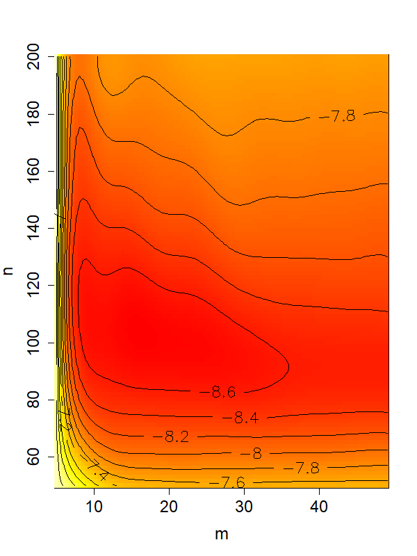

Observe that both surfaces are fairly flat across a wide swath of , excepting quick ascent (decrease in accuracy) for smaller numbers of inducing points in the left panel. The situation is similar for . Best settings are apparently input-dimension dependent. Numbers of inducing points as low as seems sufficient in 2d (top panel), whereas is needed in 8d. For borehole, it appears that larger neighborhoods are better, perhaps because the response surface is very smooth and the likelihood prefers long lengthscales (Gramacy, 2016). A setting like seems to offer good results without being too large. The situation is different for Herbie’s tooth. Here larger has deleterious effects. Its non-stationary nature demands reactivity which is proffered by smaller local neighborhood. A setting of looks good.
These are just two problems, and it is clearly not reasonable to grid-out space for all future applications. But nevertheless we have found that these rules of thumb port well to our empirical work in Section 5. Our satdrag example () and classic benchmark work well with the settings found for borehole, for example. Some ideas for automating the choice of are discussed in Section 6.