Deep Historical Borrowing Framework to Prospectively and Simultaneously Synthesize Control Information in Confirmatory Clinical Trials with Multiple Endpoints

In current clinical trial development, historical information is receiving more attention as it provides utility beyond sample size calculation. Meta-analytic-predictive (MAP) priors and robust MAP priors have been proposed for prospectively borrowing historical data on a single endpoint. To simultaneously synthesize control information from multiple endpoints in confirmatory clinical trials, we propose to approximate posterior probabilities from a Bayesian hierarchical model and estimate critical values by deep learning to construct pre-specified strategies for hypothesis testing. This feature is important to ensure study integrity by establishing prospective decision functions before the trial conduct. Simulations are performed to show that our method properly controls family-wise error rate (FWER) and preserves power as compared with a typical practice of choosing constant critical values given a subset of null space. Satisfactory performance under prior-data conflict is also demonstrated. We further illustrate our method using a case study in Immunology.

Keywords: Bayesian hierarchical model; Deep learning; Family-wise error rate control; Power preservation; Prospective algorithm

Historical control data are usually summarized as estimates of parameters needed to calculate the sample size when designing a traditional Phase III randomized clinical trial (Chow et al., 2007). This relevant information can be properly borrowed for the current trial to make it more efficient and ethical by allowing fewer patients randomized to the control group or decreasing the total sample size (Berry et al., 2010; Viele et al., 2014). Some challenges exist in applying this framework to clinical trials, especially confirmatory studies. While it is always possible to retrospectively use historical information once the new evidence is available, it is appealing to ensure study integrity by designing a prospective algorithm for leveraging historical data (Neuenschwander et al., 2010). Moving beyond the “sweet spot” where the borrowed information and the current data are similar, one needs to properly discount historical information to control the bias and the type I error rates (Viele et al., 2014).

In the context of a single endpoint, Neuenschwander et al., 2010 proposed a novel meta-analytic-predictive (MAP) approach to prospectively borrow historical information for the current trial. Schmidli et al., 2014 further developed an innovative method to approximate the MAP prior by a mixture of conjugate priors, and therefore the posterior distribution is available in a closed form. A robust MAP prior is then formulated by adding a weakly informative component to discount historical data under prior-data conflict (Schmidli et al., 2014). Moving further to confirmatory clinical trials, most use multiple endpoints to assess the effects of the study drug (Food and Drug Administration, 2017). A Bayesian hierarchical model is a natural approach to simultaneously synthesize information from multiple endpoints (Berry et al., 2010). However, taking a trial with binary endpoints as an example, additional non-trivial work is needed to generalize the MAP framework to approximate the joint prior of response rates and to investigate whether the resulting multivariate posterior distribution is available analytically.

As an alternative, we propose a two-stage Deep Neural Networks (DNN) guided algorithm to build pre-specified decision functions before initiation of the current trial. It takes advantage of the strong functional representation of DNN (Goodfellow et al., 2016; Bach, 2017; Yarotsky, 2017) to directly approximate posterior probabilities in Section 3.2, and critical values in Section 3.3. Our proposed method has several appealing features. First, it is a prospective approach in the sense that pre-trained DNN models can be locked in files before initiation of the current trial to ensure study integrity. Moreover, our method provides an accurate type I error rate control by modeling corresponding critical values. As an alternative, simulation-based type I error control by using constant critical values within a subset of the null space can be viewed as a “worst case scenario” adjustment, which leads to power loss when the type I error rate is conservative (Proschan and Hunsberger, 1995; Graf et al., 2014; Zhan et al., 2020b). More demonstration is provided in Section 4. Additionally, simulations and the case study show that our method has relatively small bias and mean squared error (MSE) under prior-data conflict by properly discounting prior information.

The remainder of this article is organized as follows. In Section 2, we introduce a Bayesian hierarchical model on control data from several historical studies. Next we propose DNN-based algorithms to approximate the posterior probabilities and critical values to build pre-specified decision functions for hypothesis testing in Section 3. Simulations in Section 4 and a case study in Section 5 are conducted to evaluate the performance of our method. Concluding remarks are provided in Section 6.

Consider a two-group randomized controlled clinical trial with $I$ ($I\geq 2$) endpoints to study the efficacy of a treatment versus placebo. We consider a setup of $I=2$ binary endpoints for illustration, but our method can be readily generalized to $I>2$ endpoints and other types of endpoints. Denote $R^{(t)}_{i,0}$ as the number of responders in the current treatment group for endpoint $i$, where $i\in\{1,\cdots,I\}$, and $n^{(t)}_{0}$ as the total number of subjects from the treatment arm in the current trial. The superscript “(t)” denotes the treatment group. For each endpoint $i$, a Beta conjugate prior is assumed on the Binomial sampling distribution with rate $\psi^{(t)}_{i,0}$,

The control data are available in the current trial and $J$ historical studies. The corresponding notations are denoted as $R^{(c)}_{i,j}$ and $n^{(c)}_{j}$, where $j=0$ indicates the current trial, $j\in\left\{1,\cdots,J\right\}$ is the index of historical study $j$, and $i\in\left\{1,\cdots,I\right\}$ refers to endpoint $i$. We consider the following Bayesian hierarchical model on the control data (Neuenschwander et al., 2010; Schmidli et al., 2014),

where $\boldsymbol{\mu}_{j}=(\mu_{1,j},\cdots,\mu_{I,j})$, for $i\in\left\{1,\cdots,I\right\}$, $j\in\left\{0,1,\cdots,J\right\}$, and $MVN(\boldsymbol{\theta},\Sigma)$ denotes a multivariate Normal distribution with mean vector $\boldsymbol{\theta}$ and variance-covariance matrix $\Sigma$. A vague prior is assumed on $\boldsymbol{\theta}$, and an $InverseWishart(\Sigma_{0},k)$ prior is assigned to the variance-covariance matrix $\Sigma$ with positive definite $I\times I$ matrix $\Sigma_{0}$ and degrees of freedom $k\geq I$. The expectation of a $Wishart(\Sigma_{0},k)$ is $k\left(\Sigma_{0}\right)^{-1}$, and therefore $\Sigma_{0}/k$ is a prior guess for $\Sigma$. We use $\boldsymbol{D}_{H}=\left[R^{(c)}_{i,j},n^{(c)}_{j},i\in\left\{1,\cdots,I\right\},j\in\left\{1,\cdots,J\right\}\right]$ to denote control information in $J$ historical studies, and $\boldsymbol{D}_{N}=\left[R^{(c)}_{i,0},n^{(c)}_{0},R^{(t)}_{i,0},n^{(t)}_{0},i\in\left\{1,\cdots,I\right\}\right]$ as data in the current new trial.

Our quantity of interest is the posterior probability of observing a promising treatment effect in the current trial,

where $\theta_{i}$ is a pre-specified constant for endpoint $i$. The decision function of rejecting the null hypothesis pertaining to endpoint $i$ is if $S_{i}>\widetilde{c}_{i}$. The critical value $\widetilde{c}_{i}$ can interpreted as a threshold to claim a significant treatment effect in the $i$th endpoint with controlled type I error rates. The computation of $\widetilde{c}_{i}$ is studied in the next section to control the family-wise error rate (FWER) at a nominal level $\alpha$. We denote $\boldsymbol{S}=(S_{1},\cdots,S_{I})$ as a vector of those posterior probabilities.

Since the posterior probabilities $\boldsymbol{S}$ in (3) usually do not have closed forms, we estimate them empirically by a large number of Monte Carlo samples. Specifically, posterior samples $\psi_{i,0}^{(t)}$ are simulated from the conjugate prior model in (1), and posterior samples $\psi_{i,0}^{(c)}$ in the Bayesian hierarchical model (2) are obtained by the Markov chain Monte Carlo (MCMC) method based on current trial data (Berry et al., 2010). However, it is appealing to build a prospective algorithm before conducting the current new trial to ensure the study integrity. In studies with a single binary endpoint ($I=1$), Schmidli et al., 2014 proposed a novel approach by approximating the Meta Analytic Predictive (MAP) prior $p\left\{\psi^{(c)}_{i,0}|\boldsymbol{D}_{H}\right\}$ with a mixture of Beta distributions, and hence the posterior distribution $p\left\{\psi^{(c)}_{i,0}|\boldsymbol{D}_{H},\boldsymbol{D}_{N}\right\}$ becomes a weighted average of Beta distributions. In the context of multiple endpoints ($I\geq 2$), a Bayesian hierarchical model in (2) is a natural approach to simultaneously synthesize control information (Berry et al., 2010). Even if one can utilize several base distributions to approximate the multivariate prior $p\left\{\boldsymbol{\psi}_{0}^{(c)}|\boldsymbol{D}_{H}\right\}$, where $\boldsymbol{\psi}_{0}^{(c)}=\left\{\psi^{(c)}_{1,0},\cdots,\psi^{(c)}_{I,0}\right\}$, the joint posterior probability $\boldsymbol{S}$ does not necessarily have an analytic closed form.

As an alternative, we propose to directly approximate $\boldsymbol{S}$ based on observed historical data $\boldsymbol{D}_{H}$ and varying simulated new trial data $\boldsymbol{D}_{N}$ by deep neural networks (DNN) in the study design stage. After collecting results from the current trial, one can instantly compute $\boldsymbol{S}$ and conduct downstream hypothesis testing based on pre-specified approximation functions.

In this section, we first provide a short review on DNN in Section 3.1, and then introduce our DNN guided historical borrowing framework by directly approximating the posterior probabilities and posterior means in Section 3.2. In Section 3.3, we further estimate corresponding critical values by DNNs to control FWER in the strong sense. The hypothesis testing based on observed current trial data is discussed in Section 3.4.

In this section, we conduct simulation studies to evaluate the performance of our proposed method, and compare it with the Meta-Analytic-Prior (MAP) approach (Neuenschwander et al., 2010; Schmidli et al., 2014). Suppose that there are two endpoints ($I=2$) to be evaluated in a randomized clinical trial comparing a treatment versus placebo with equal sample size $n_{0}^{(c)}=n_{0}^{(t)}=150$. The control information is also available in $J=6$ historical studies with sample sizes $100,100,200,200,300$, and $300$, with the response rates $0.4$ and $0.3$ for the two endpoints. We consider FWER to be controlled at $\alpha=0.05$.

We consider historical control data as in Table 1. The number of responders $R^{(c)}_{i,j}$ for endpoint $i$, $i=1,2$, study $j$, $j=1,\cdots,6$ is simulated from a Binomial distribution with rate $0.4$ for endpoint $i=1$ and $0.3$ for endpoint $i=2$. The empirical correlation of estimated response rate $R^{(c)}_{i,j}/n^{(c)}_{j}$ between two endpoints is $0.01$. Additional simulation studies with an empirical correlation around $0.5$ are conducted in the Supplemental Materials and demonstrate consistent findings.

To implement our DNN-based method, we first approximate the posterior probability $\boldsymbol{S}$ in (3) based on Algorithm 1 with training data size $B=8,000$. Its training input data $\boldsymbol{M}=\left\{{R}^{(c)}_{1,0},{R}^{(c)}_{2,0},{R}^{(t)}_{1,0},{R}^{(t)}_{2,0}\right\}$ are drawn from Binomial distributions with rates $\left\{{\psi}^{(c)}_{1,0},{\psi}^{(c)}_{2,0},{\psi}^{(t)}_{1,0},{\psi}^{(t)}_{2,0}\right\}$, which are further simulated from the following $4$ patterns with equal size $B/4=2,000$,

1. 1.

   ${\psi}^{(c)}_{1,0}\sim\mathrm{Unif}(0.2,0.7);\>\>\>{\psi}^{(c)}_{2,0}\sim\mathrm{Unif}(0.1,0.6);\>\>\>{\Delta}_{1,0}=0;\>\>\>{\Delta}_{2,0}=0$,

2. 2.

   ${\psi}^{(c)}_{1,0}\sim\mathrm{Unif}(0.2,0.7);\>\>\>{\psi}^{(c)}_{2,0}\sim\mathrm{Unif}(0.1,0.6);\>\>\>{\Delta}_{1,0}\sim\mathrm{Unif}(-0.1,0.2);\>\>\>{\Delta}_{2,0}=0$,

3. 3.

   ${\psi}^{(c)}_{1,0}\sim\mathrm{Unif}(0.2,0.7);\>\>\>{\psi}^{(c)}_{2,0}\sim\mathrm{Unif}(0.1,0.6);\>\>\>{\Delta}_{1,0}=0;\>\>\>{\Delta}_{2,0}\sim\mathrm{Unif}(-0.1,0.2)$,

4. 4.

   ${\psi}^{(c)}_{1,0}\sim\mathrm{Unif}(0.2,0.7);\>\>\>{\psi}^{(c)}_{2,0}\sim\mathrm{Unif}(0.1,0.6);\>\>\>{\Delta}_{1,0}\sim\mathrm{Unif}(-0.1,0.2);\>\>\>{\Delta}_{2,0}\sim\mathrm{Unif}(-0.1,0.2)$,

where $\mathrm{Unif}$ denotes the Uniform distribution, and the treatment response rates are calculated at ${\psi}^{(t)}_{i,0}={\psi}^{(c)}_{i,0}+{\Delta}_{i,0}$ for $i=1,2$. The ranges of above Uniform distributions are determined based on previous knowledge that ${\psi}^{(c)}_{1,0}$ is between $0.2$ and $0.7$, while ${\psi}^{(c)}_{2,0}$ is within $0.1$ and $0.6$. The Uniform distribution can be substituted by other sampling distributions, e.g., flat normal distribution. For this simulation study, the training data size $B=8,000$ is sufficient to give DNN satisfactory performance, for example training MSE less than $10^{-3}$. It can be increased to accommodate more distinct training features, as in the next section of case study.

Next we obtain posterior samples of ${\psi}_{i,0}^{(c)}$ from model (2) based on the Markov chain Monte Carlo (MCMC) method implemented by the R package R2jags (Su and Yajima, 2015). We put a vague prior on $\boldsymbol{\theta}$ following a Normal distribution with mean zero and precision $0.01$, and an $\mathrm{InverseWishart}(\Sigma_{0},k)$ prior for $\Sigma$ with $\Sigma_{0}$ as a unit diagonal matrix and $k=I+1$. The convergence of the MCMC algorithm is checked by the criteria of $\widehat{R}<1.01$ among $3$ chains, where $\widehat{R}$ is the ratio of between-chain versus within-chain variability (Gelman et al., 1992; Berry et al., 2010). The posterior distribution of ${\psi}_{i,0}^{(t)}$ is a Beta distribution with a non-informative Beta prior $a_{i}=b_{i}=1$ based on the Beta-Binomial conjugate model in (1). Our posterior probability $S_{i}$ in (3) is evaluated by $30,000$ posterior samples with $\theta_{i}=0$. In Step 2 of selecting a proper DNN structure, we consider a pool of four candidate structures: $H_{l}=2$ hidden layers with $H_{n}=40$ nodes per layer, $H_{l}=2$ and $H_{n}=60$, $H_{l}=3$ and $H_{n}=40$, $H_{l}=3$ and $H_{n}=60$. The batch size $H_{b}$ is $100$, and the number of training epochs $H_{e}$ is $1,000$ with dropout rate $H_{d}=0.1$. The above parameters are used throughout this article unless specified otherwise. In this simulation study, we choose a DNN structure with $H_{l}=2$ hidden layers, $H_{n}=60$ nodes per layer with the smallest validation MSE among four candidates. This DNN structure is utilized in Algorithm 2 as well. From the final fitting at Step 3, we obtain DNN $\widehat{\boldsymbol{S}}=F_{S}(\boldsymbol{M};\widehat{\boldsymbol{\phi}})$ to estimate $\boldsymbol{S}$ in (3).

In Algorithm 2 of approximating the critical values, we simulate $B_{1}=B_{2}=B_{12}=2,000$ datasets to reflect patterns of $H_{1}$ in (4), $H_{2}$ in (5) and $H_{12}$ in (6),

1. 1.

   ${\psi}^{(c,t)}_{1,0}\sim\mathrm{Unif}(0.2,0.7);\>\>\>{\psi}^{(c)}_{2,0}\sim\mathrm{Unif}(0.1,0.6);\>\>\>{\Delta}_{2,0}\sim\mathrm{Unif}(-0.1,0.2);\>\>\>{\psi}^{(t)}_{2,0}={\psi}^{(c)}_{2,0}+{\Delta}_{2,0}$,

2. 2.

   ${\psi}^{(c)}_{1,0}\sim Unif(0.2,0.7);\>\>\>{\Delta}_{1,0}\sim\mathrm{Unif}(-0.1,0.2);\>\>\>{\psi}^{(t)}_{1,0}={\psi}^{(c)}_{1,0}+{\Delta}_{1,0};\>\>\>{\psi}^{(c,t)}_{2,0}\sim\mathrm{Unif}(0.1,0.6)$,

3. 3.

   ${\psi}^{(c,t)}_{1,0}\sim\mathrm{Unif}(0.2,0.7);\>\>\>{\psi}^{(c,t)}_{2,0}\sim\mathrm{Unif}(0.1,0.6)$.

The number of iterations of calculating critical values are $B^{\prime}_{1}=B^{\prime}_{2}=B^{\prime}_{12}=100,000$.

We implement the Meta-Analytic-Predictive (MAP) priors (Neuenschwander et al., 2010) and two robust MAP priors with a weight of $w=50\%$ and $w=80\%$ non-informative component (Schmidli et al., 2014) by the R package RBesT (Weber, 2020). These methods handle data from each endpoint separately, instead of modeling them jointly as in our model (2). The setup follows their default settings with a weakly informative Half-Normal $(0,1)$ prior on the standard deviation of the logit of the response rate (Weber et al., 2019). Hypothesis testing is also based on posterior probabilities $S_{i}$, but the constant critical values $\widetilde{c}$ are chosen by a grid search method to control testing type I error rates not exceeding $\alpha=0.05$ within a certain range of null response rates in the following Table 2.

In Table 2, we first evaluate the error rates of falsely rejecting $H_{12}$, $H_{1}$ or $H_{2}$ under the global null hypothesis where $\Delta_{1,0}=\Delta_{2,0}=0$. The number of iterations in testing is $100,000$. Our proposed method has relatively accurate control on three error rates at $\alpha=0.05$ across three scenarios with varying $\psi_{1,0}^{(c)}$ and $\psi_{2,0}^{(c)}$. For MAP and two robust MAPs, we choose their constant critical values $\tilde{c}$’s (introduced in Section 2) at $0.9977$, $0.9927$, and $0.9867$, respectively, by the grid search method such that the probability of rejecting $H_{12}$ reaches the nominal level of $0.05$ under the “worst case scenario” with $\psi_{1,0}^{(c)}=0.5$ and $\psi_{2,0}^{(c)}=0.4$. This scenario has the largest type I error rate given the same critical value under the null space evaluated in Table 2. This simulation-based type I error rate control ensures that FWER does not exceed $\alpha$ under all three null cases, but leads to conservative error rates and potential power loss in some cases as evaluated later. The critical value $\tilde{c}=0.9977$ of MAP is interpreted as a cutoff to claim a significant treatment effect based on endpoint $i$, because we reject the null hypothesis pertaining to endpoint $i$ if its posterior probability $S_{i}$ in (3) is larger than $\tilde{c}$ based on Section 2.

Under a single null hypothesis where only a single $\Delta_{i}$ is equal to zero, the error rate happens when this particular true null hypothesis is erroneously rejected. All methods control this error rate well below $\alpha$. When it comes to alternative hypotheses, our method has a much higher power of rejecting each elementary null hypothesis, and a higher power of rejecting at least one of them than MAP and two RMAPs under $\psi_{1,0}^{(c)}=0.3,\psi_{2,0}^{(c)}=0.2$ and $\psi_{1,0}^{(c)}=0.4,\psi_{2,0}^{(c)}=0.3$. This is mainly due to the conservative type I error of using a constant critical value for MAP and RMAPs. When response rates are higher at $\psi_{1,0}^{(c)}=0.5,\psi_{2,0}^{(c)}=0.4$, MAP usually has the best power performance, followed by our DNN method, and then two RMAPs. Note that there are two scenarios with prior-data conflict given that historical control rates are $0.4$, $0.3$ for the first and the second endpoint, respectively.

Table 3 presents the bias and Table 4 shows the root of mean squared error (RMSE) of posterior means of $\psi_{1,0}^{(c)}$ and $\psi_{2,0}^{(c)}$. In scenarios where the current control rates and historical rates are consistent at $0.4$ for the first endpoint and $0.3$ for the second endpoint, all methods have small biases, and MAP has the smallest RMSE. Under cases with prior-data conflict, DNN and two RMAPs have better bias than MAP, and moreover DNN has the smallest RMSE. The overall conclusion is that our DNN-based method enjoys the robustness of RMAP under prior-data conflict, and preserves power by modeling critical values as compared with MAP and RMAP by using constant critical values.

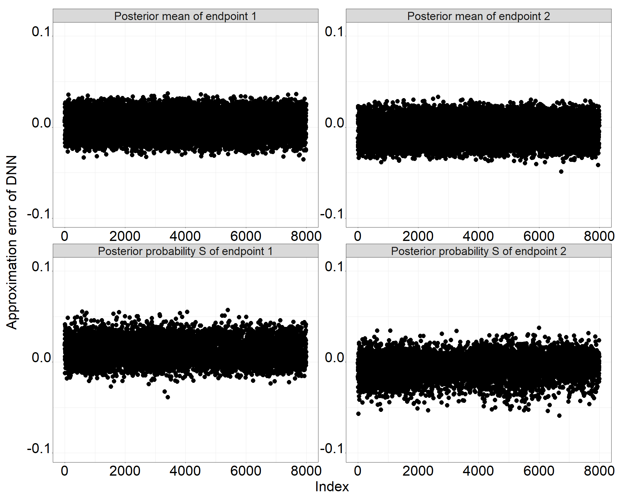
Figure 3 shows the approximation errors of DNN in estimating posterior means of $\psi_{1,0}^{(c)}$ and $\psi_{2,0}^{(c)}$, and posterior probabilities $S_{1}$ and $S_{2}$ in (3) from $B=8,000$ training data. The MSE from DNN training is approximately $0.001$. Errors are relatively larger in approximating $S_{1}$ and $S_{2}$ from (3), because their training labels have more randomness in the Monte Carlo estimates as compared with the empirical posterior means of $\psi^{(c)}_{1,0}$ and $\psi^{(c)}_{2,0}$.

References

- Bach, (2017) Bach, F. (2017). Breaking the curse of dimensionality with convex neural networks. The Journal of Machine Learning Research, 18(1):629–681.
- Berry et al., (2010) Berry, S. M., Carlin, B. P., Lee, J. J., and Muller, P. (2010). Bayesian adaptive methods for clinical trials. CRC press.
- Bretz et al., (2016) Bretz, F., Hothorn, T., and Westfall, P. (2016). Multiple comparisons using R. CRC Press.
- Chollet and Allaire, (2018) Chollet, F. and Allaire, J. J. (2018). Deep Learning with R. Manning Publications Co., Greenwich, CT, USA.
- Chow et al., (2007) Chow, S.-C., Wang, H., and Shao, J. (2007). Sample size calculations in clinical research. CRC press.
- Food and Drug Administration, (2017) Food and Drug Administration (2017). Multiple endpoints in clinical trials guidance for industry. https://www.fda.gov/downloads/drugs/guidancecomplianceregulatoryinformation/ guidances/ucm536750.pdf.
- Gelman et al., (1992) Gelman, A., Rubin, D. B., et al. (1992). Inference from iterative simulation using multiple sequences. Statistical Science, 7(4):457–472.
- Goodfellow et al., (2016) Goodfellow, I., Bengio, Y., and Courville, A. (2016). Deep learning. MIT press.
- Graf et al., (2014) Graf, A. C., Bauer, P., Glimm, E., and Koenig, F. (2014). Maximum type 1 error rate inflation in multiarmed clinical trials with adaptive interim sample size modifications. Biometrical Journal, 56(4):614–630.
- Hinton et al., (2012) Hinton, G., Srivastava, N., and Swersky, K. (2012). Neural networks for machine learning. Coursera, video lectures, 307.
- Langley et al., (2014) Langley, R. G., Elewski, B. E., Lebwohl, M., Reich, K., Griffiths, C. E., Papp, K., Puig, L., Nakagawa, H., Spelman, L., Sigurgeirsson, B., et al. (2014). Secukinumab in plaque psoriasis—results of two phase 3 trials. New England Journal of Medicine, 371(4):326–338.
- Neuenschwander et al., (2010) Neuenschwander, B., Capkun-Niggli, G., Branson, M., and Spiegelhalter, D. J. (2010). Summarizing historical information on controls in clinical trials. Clinical Trials, 7(1):5–18.
- Paul et al., (2015) Paul, C., Lacour, J.-P., Tedremets, L., Kreutzer, K., Jazayeri, S., Adams, S., Guindon, C., You, R., Papavassilis, C., and Group, J. S. (2015). Efficacy, safety and usability of secukinumab administration by autoinjector/pen in psoriasis: a randomized, controlled trial (juncture). Journal of the European Academy of Dermatology and Venereology, 29(6):1082–1090.
- Proschan and Hunsberger, (1995) Proschan, M. A. and Hunsberger, S. A. (1995). Designed extension of studies based on conditional power. Biometrics, pages 1315–1324.
- Schmidli et al., (2014) Schmidli, H., Gsteiger, S., Roychoudhury, S., O’Hagan, A., Spiegelhalter, D., and Neuenschwander, B. (2014). Robust meta-analytic-predictive priors in clinical trials with historical control information. Biometrics, 70(4):1023–1032.
- Su and Yajima, (2015) Su, Y.-S. and Yajima, M. (2015). R2jags: Using R to Run ’JAGS’. R package version 0.5-7.
- Tamhane and Gou, (2018) Tamhane, A. C. and Gou, J. (2018). Advances in p-value based multiple test procedures. Journal of Biopharmaceutical Statistics, 28(1):10–27.
- Viele et al., (2014) Viele, K., Berry, S., Neuenschwander, B., Amzal, B., Chen, F., Enas, N., Hobbs, B., Ibrahim, J. G., Kinnersley, N., Lindborg, S., et al. (2014). Use of historical control data for assessing treatment effects in clinical trials. Pharmaceutical Statistics, 13(1):41–54.
- Weber, (2020) Weber, S. (2020). RBesT: R Bayesian Evidence Synthesis Tools. R package version 1.6-0.
- Weber et al., (2019) Weber, S., Li, Y., Seaman, J., Kakizume, T., and Schmidli, H. (2019). Applying meta-analytic predictive priors with the R Bayesian evidence synthesis tools. arXiv preprint arXiv:1907.00603.
- Yarotsky, (2017) Yarotsky, D. (2017). Error bounds for approximations with deep ReLU networks. Neural Networks, 94:103–114.
- (22) Zhan, T., Hartford, A., Kang, J., and Offen, W. (2020a). Optimizing graphical procedures for multiplicity control in a confirmatory clinical trial via deep learning. Statistics in Biopharmaceutical Research, pages 1–11.
- (23) Zhan, T., Zhang, H., Hartford, A., and Mukhopadhyay, S. (2020b). Modified goldilocks design with strict type I error control in confirmatory clinical trials. Journal of Biopharmaceutical Statistics, 30(5):821–833.