跳到论文正文
W Papers独立论文阅读器 arXiv:2008.12758 论文正文 计算阅读时间 · 0%
引用这篇论文根据当前论文元数据生成,正式投稿前建议核对。


License: arXiv.org perpetual non-exclusive license
arXiv:2008.12758v1 [gr-qc] 28 Aug 2020

Stealth spontaneous spinorization of relativistic stars

Masato Minamitsuji Affiliation: Center for Astrophysics and Gravitation (CENTRA), Instituto Superior Técnico, University of Lisbon, Lisbon 1049-001, Portugal.
Abstract

We investigate the behavior of the Dirac spinor fields in general relativistic high density stellar backgrounds and the possibility of spontaneous spinorization which is analogous to spontaneous scalarization. We consider the model with the modified kinetic term of the Dirac field by the insertion of the fifth gamma matrix γ^5{\hat{\gamma}}^{5} and the conformal coupling of the Dirac spinor field to the matter sector, which would lead to the tachyonic growth of the Dirac spinor field in the high density compact stellar backgrounds. In order to obtain the static and spherically symmetric solutions, we have to consider the two Dirac fields at the same time. We show that in the constant density stellar backgrounds our model gives rise to the nontrivial solutions of the Dirac spinor fields with any number of nodes, where one mode has one more node than the other. We also show that at the leading order all the components of the effective energy-momentum tensor of the Dirac spinor fields, after the summation over the two fields, vanish for any separable time-dependent ansatz of the Dirac spinor fields in any static and spherically symmetric spacetime backgrounds, indicating that spontaneous spinorization takes place as a stealth process in the static and spherically symmetric spacetime with any number of nodes, which would be quenched by nonlinear effects and leave no observable effects.

Keywords: 
Higher-dimensional Gravity, Modified Theories of Gravity, Cosmology
pacs
04.50.-h, 04.50.Kd, 98.80.-k

I Introduction

Einstein’s general relativity has been tested by various experiments and observations on the scales from the Solar System to binary pulsars Will 2014, with the dawn of gravitational wave observations, and the frontier for testing genetal relativity will expand to strong gravity regimes Berti et al. 2015; Berti et al. 2018a; Berti et al. 2018b. A potentially interesting phenomenon which could be tested in strong gravity regimes is spontaneous scalarization which allows for large deviations from general relativity via the tachyonic growth of the scalar field inside relativistic stars Damour and Esposito-Farèse 1993. In scalar-tensor systems with the conformal coupling to matter, a stellar solution in general relativity with the vanishing scalar field ϕ=0\phi=0 suffers from a tachyonic instability, leading to a relativistic star solution with a nontrivial profile of the scalar field  Damour and Esposito-Farèse 1996; Harada 1997; Harada 1998; Novak 1998; Palenzuela et al. 2014; Sampson et al. 2014; Pani and Berti 2014; Silva et al. 2015.

The idea of spontaneous scalarization may be extended to other field species such as vector and spinor fields. The possibility of spontaneous vectorization triggered by the tachyonic instability of the vector field has been studied recently in Refs. Ramazanoğlu 2017; Ramazanoğlu 2019; Annulli et al. 2019; Ramazanoğlu and Ünlütürk 2019; Kase et al. 2020; Minamitsuji 2020. Refs. Annulli et al. 2019; Kase et al. 2020 have studied the model with nonminimal couplings of the vector field to the spacetime curvature, and constructed static and spherically symmetric relativistic star solutions with nontrivial vector field profiles, which would be formed via the selected choice of the initial conditions rather via the instability of the general relativistic solutions. On the other hand, the analyses from the Jordan frame viewpoint have been presented in Refs. Ramazanoğlu 2017; Minamitsuji 2020, and showed that spontaneous vectorization could happen as in the same manner as spontaneous scalarization via the vector conformal coupling to matter.

In this paper, we will explore the similar phenomena in the fermionic sectors, namely, spontaneous spinorization. This possibility was discussed Ramazano˘glu 2018 at the first time. For clarification, we start with the theory of the standard massive Dirac spinor field ψ\psi in the Minkowski spacetime given by

S(ψ)=∫d4​X​[12​(ψ¯​γ^a​∂aψ−(∂aψ¯)​γ^a​ψ)−m​ψ¯​ψ],\displaystyle S_{(\psi)}=\int d^{4}X\left[\frac{1}{2}\left({\bar{\psi}}{\hat{\gamma}}^{a}\partial_{a}\psi-\left(\partial_{a}{\bar{\psi}}\right){\hat{\gamma}}^{a}\psi\right)-m{\bar{\psi}}\psi\right], (1)

where the indices a,b,c,⋯=0,1,2,3a,b,c,\cdots=0,1,2,3 run the four-dimensional Minkowski spacetime with the metric ηa​b\eta_{ab},

d​s^2:=ηa​b​d​Xa​d​Xb=−d​(X0)2+d​(X1)2+d​(X2)2+d​(X3)2,\displaystyle d{\hat{s}}^{2}:=\eta_{ab}dX^{a}dX^{b}=-d(X^{0})^{2}+d(X^{1})^{2}+d(X^{2})^{2}+d(X^{3})^{2}, (2)

∂a:=∂/∂Xa\partial_{a}:=\partial/\partial X^{a} is the partial derivative with respect to the coordinate XaX^{a}, mm is the constant mass parameter, the Dirac gamma matrices in the Minkowski spacetime γ^a{\hat{\gamma}}^{a} satisfy the anticommutation relations

{γ^a,γ^b}=2​ηa​b​I4×4,\displaystyle\{{\hat{\gamma}}^{a},{\hat{\gamma}}^{b}\}=2\eta^{ab}I_{4\times 4}, (3)

with I4×4I_{4\times 4} being the 4×44\times 4 unit matrix, and ψ¯:=−i​ψ†​γ^0\bar{\psi}:=-i\psi^{\dagger}{\hat{\gamma}}^{0} is the Dirac adjoint of ψ\psi. Varying the action (1) with respect to ψ¯\bar{\psi} yields the usual Dirac equation (γ^a∂a−m)ψ=0\left({\hat{\gamma}}^{a}\partial_{a}-m\right)\psi=0. Assuming that the solution is given by the Fourier form ψ=∫d​p^​u​(p^)​ei​p^a​Xa\psi=\int d{\hat{p}}\,u({\hat{p}})e^{i{\hat{p}}_{a}X^{a}}, where p^a=(−E^,p^→){\hat{p}}_{a}=(-{\hat{E}},\vec{\hat{p}}) denotes the four-momentum with E^{\hat{E}} and p^→\vec{\hat{p}} being the energy and linear momentum, respectively, each partial mode function u⁡(p)u(p) satisfies (i​γ^a​p^a−m)​u​(p)=0\left(i{\hat{\gamma}}^{a}{\hat{p}}_{a}-m\right)u(p)=0. Acting γ^a∂a+m{\hat{\gamma}}^{a}\partial_{a}+m from the left side leads to 0=[−12​{γ^a,γ^b}​p^a​p^b−m2]​u​(p^)=[−ηa​b​p^a​p^b−m2]​u​(p^)=[E^2−|p^→|2−m2]​u​(p^)0=\left[-\frac{1}{2}\left\{{\hat{\gamma}}^{a},{\hat{\gamma}}^{b}\right\}{\hat{p}}_{a}{\hat{p}}_{b}-m^{2}\right]u({\hat{p}})=\left[-\eta^{ab}{\hat{p}}_{a}{\hat{p}}_{b}-m^{2}\right]u({\hat{p}})=\left[{\hat{E}}^{2}-|\vec{\hat{p}}|^{2}-m^{2}\right]u({\hat{p}}), and hence we obtain the standard dispersion relation E^2=|p^→|2+m2{\hat{E}}^{2}=|\vec{\hat{p}}|^{2}+m^{2}.

We then consider the theory of the Dirac spinor field in the four-dimensional Minkowski spacetime given by

S(ψ)=∫d4​X​[12​(ψ¯​γ^5​γ^a​∂aψ−∂aψ¯​γ^5​γ^a​ψ)−M​ψ¯​ψ],\displaystyle S_{(\psi)}=\int d^{4}X\left[\frac{1}{2}\left({\bar{\psi}}{\hat{\gamma}}^{5}{\hat{\gamma}}^{a}\partial_{a}\psi-\partial_{a}{\bar{\psi}}{\hat{\gamma}}^{5}{\hat{\gamma}}^{a}\psi\right)-M{\bar{\psi}}\psi\right], (4)

where we have defined

γ^5:=i​γ^0​γ^1​γ^2​γ^3,{γ^a,γ^5}=0,γ^5⋅γ^5=I4×4,\displaystyle{\hat{\gamma}}^{5}:=i{\hat{\gamma}}^{0}{\hat{\gamma}}^{1}{\hat{\gamma}}^{2}{\hat{\gamma}}^{3},\qquad\left\{{\hat{\gamma}}^{a},{\hat{\gamma}}^{5}\right\}=0,\qquad{\hat{\gamma}}^{5}\cdot{\hat{\gamma}}^{5}=I_{4\times 4}, (5)

and MM is a constant. *1*1 *1 The alternative theory which gives the same equation of motion for ψ\psi is given by S(ψ)=∫d4​X​[12​(ψ¯​γ^a​∂aψ−∂aψ¯​γ^a​ψ)−M​ψ¯​γ^5​ψ].\displaystyle S_{(\psi)}=\int d^{4}X\left[\frac{1}{2}\left({\bar{\psi}}{\hat{\gamma}}^{a}\partial_{a}\psi-\partial_{a}{\bar{\psi}}{\hat{\gamma}}^{a}\psi\right)-M{\bar{\psi}}{\hat{\gamma}}^{5}\psi\right]. (6) As argued in Refs. Jentschura and Wundt 2012; Ramazano˘glu 2018, however, the variation of Eq. (6) leads to the inconsistent equation for ψ¯{\bar{\psi}} (see Appendix A). Variation of Eq. (4) yields the modified Dirac equation

(γ^5γ^a∂a−M)ψ=0.\displaystyle\left({\hat{\gamma}}^{5}{\hat{\gamma}}^{a}\partial_{a}-M\right)\psi=0. (7)

Assuming the form of the solution ψ=∫d​p^​v​(p^)​ei​p^a​Xa\psi=\int d{\hat{p}}\,v({\hat{p}})e^{i{\hat{p}}_{a}X^{a}}, each mode satisfies (i​γ^a​p^a−M​γ^5)​v​(p^)=0.\left(i{\hat{\gamma}}^{a}{\hat{p}}_{a}-M{\hat{\gamma}}^{5}\right)v({\hat{p}})=0. Acting γ^a∂a−Mγ^5{\hat{\gamma}}^{a}\partial_{a}-M{\hat{\gamma}}^{5} from the left side results in 0=[−γ^a​γ^b​p^a​p^b+i​M​{γ^a,γ^5}​p^a+M2]​v​(p^)=[−12​{γ^a,γ^b}​p^a​p^b+M2]​v​(p^)=[−ηa​b​p^a​p^b+M2]​v​(p^)=[E^2−|p^→|2+M2]​v​(p^)0=\left[-{\hat{\gamma}}^{a}{\hat{\gamma}}^{b}{\hat{p}}_{a}{\hat{p}}_{b}+iM\left\{{\hat{\gamma}}^{a},{\hat{\gamma}}^{5}\right\}{\hat{p}}_{a}+M^{2}\right]v({\hat{p}})=\left[-\frac{1}{2}\left\{{\hat{\gamma}}^{a},{\hat{\gamma}}^{b}\right\}{\hat{p}}_{a}{\hat{p}}_{b}+M^{2}\right]v({\hat{p}})=\left[-\eta^{ab}{\hat{p}}_{a}{\hat{p}}_{b}+M^{2}\right]v(\hat{p})=\left[{\hat{E}}^{2}-|\vec{\hat{p}}|^{2}+M^{2}\right]v({\hat{p}}), and hence the dispersion relation is modified as E^2=|p^→|2−M2{\hat{E}}^{2}=|\vec{\hat{p}}|^{2}-M^{2}. Thus, the modes of |p^→|<M|\vec{\hat{p}}|<M suffer from the tachyonic instability. If the constant MM is promoted to a position-dependent function M⁡(xμ)M(x^{\mu}), one may be able to make the modes tachyonic only locally, for instance, in the vicinity of black holes and compact stars. This is the basic idea behind spontaneous spinorization Ramazano˘glu 2018.

We will consider the model with the conformal coupling of the Dirac spinor field to matter (see Eqs. (8)-(10)), and study the behavior of the Dirac spinor field inside the high density compact stars. We will show that the modified kinetic term by the insertion of γ^5{\hat{\gamma}}^{5} (9) and the conformal coupling (10) would lead to the tachyonic growth of the Dirac spinor field inside the high density compact stellar backgrounds, where the parameter MM is replaced by the trace of the energy-momentum tensor of the matter T(m)​μμ{T}^{(m)\mu}{}_{\mu}. By the analysis in the constant density stellar backgrounds, we will show that this coupling gives rise to the nontrivial profiles of the Dirac spinor field with any number of nodes. We will also show that up to the quadratic order of the Dirac spinor fields and their adjoints all the components of the effective energy-momentum tensor of the Dirac field vanish in any static and spherically symmetric stellar backgrounds. Thus, even if the amplitude of the Dirac spinor field grows with time, it will not affect the spacetime geometry, indicating that spontaneous spinorization happens as a stealth process. *2*2 *2 The term “stealth” has been used to describe the Schwarzschild/ Kerr black hole solutions in the scalar-tensor or vector-tensor theories where the scalar or vector field with the nontrivial profile does not backreact on the spacetime geometry (see e.g., Refs. Babichev and Charmousis 2014; Chagoya et al. 2016; Minamitsuji and Motohashi 2018; Takahashi and Motohashi 2020). This happens in the case that all the components of the effective energy-momentum tensor of the scalar or vector field automatically vanish in the right-hand side of the gravitational equations of motion. We will dub this stealth spontaneous spinorization. Since the vanishing effective energy-momentum tensor holds in any static and spherically background, stealth spontaneous spinorization would happen for any equation of state of matter. The tachyonic growth of the Dirac spinor field may be quenched by nonlinear effects, and would not affect the spacetime geometry around relativistic stars, and not leave any observable consequences.

This paper is organized as follows: in Sec. II, we will introduce the model for spontaneous spinorization with the coupling of the Dirac spinor field to the matter. In Sec. III, we will review the general properties of the Dirac spinor field in the static and spherically symmetric spacetimes. In Sec. IV, we will analyze the Dirac spinor field s in the constant density stellar backgrounds. In Sec. V, we will show that the effective energy-momentum tensor of the Dirac fields vanish, and discuss the implications for spontaneous spinorization. The last Sec. VI will be devoted to giving a brief summary and conclusion.

II Model

We consider the theory composed of the metric tensor gμ​νg_{\mu\nu} and the Dirac spinor field ψ\psi,

S\displaystyle S =\displaystyle= ∫d4​x​[−g​(R2​κ2+L(ψ))+−g~​L(m)​[g~μ​ν,Ψ]],\displaystyle\int d^{4}x\left[\sqrt{-g}\left(\frac{R}{2\kappa^{2}}+L_{(\psi)}\right)+\sqrt{-{\tilde{g}}}L_{(m)}\left[{\tilde{g}}_{\mu\nu},\Psi\right]\right], (8)

with the modified kinetic term

L(ψ):=12​[ψ¯​γ^5​γμ​Dμ​ψ−(Dμ​ψ¯)​γ^5​γμ​ψ],\displaystyle{L}_{(\psi)}:=\frac{1}{2}\left[{\bar{\psi}}{\hat{\gamma}}^{5}{\gamma}^{\mu}D_{\mu}\psi-\left(D_{\mu}{\bar{\psi}}\right){\hat{\gamma}}^{5}{\gamma}^{\mu}\psi\right], (9)

where the induces μ,ν,⋯\mu,\nu,\cdots run the physical spacetime with the metric gμ​νg_{\mu\nu}, κ2=8​π​G/c4\kappa^{2}=8\pi G/c^{4} with the gravitational constant GG and the speed of light cc (we will set c=1c=1 unless necessary), RR is the scalar curvature associated with gμ​νg_{\mu\nu}, ψ¯:=−i​ψ†​γ^0\bar{\psi}:=-i\psi^{\dagger}{\hat{\gamma}}^{0} is the Dirac adjoint of ψ\psi, γ^a{\hat{\gamma}}^{a} denotes the Dirac gamma matrices satisfying the anticommutation relations Eq. (3), γμ:=eaμ​γ^a\gamma^{\mu}:=e^{\mu}_{a}{\hat{\gamma}}^{a} with eaμe^{\mu}_{a} being the tetrad field satisfying gμ​ν​eaμ​ebν=ηa​bg_{\mu\nu}e^{\mu}_{a}e^{\nu}_{b}=\eta_{ab}, Dμ​ψ:=∂μψ+Γμ​ψD_{\mu}\psi:=\partial_{\mu}\psi+\Gamma_{\mu}\psi and Dμ​ψ¯:=∂μψ¯−ψ¯​ΓμD_{\mu}{\bar{\psi}}:=\partial_{\mu}{\bar{\psi}}-{\bar{\psi}}\Gamma_{\mu} denote the covariant derivatives with the spin connection Γμ:=(1/8)​[γ^a,γ^b]​eaν​∇μeb​ν\Gamma_{\mu}:=(1/8)\left[{\hat{\gamma}}^{a},{\hat{\gamma}}^{b}\right]e_{a}^{\nu}\nabla_{\mu}e_{b\nu}, g~μ​ν{\tilde{g}}_{\mu\nu} represents the Jordan frame metric related to the Einstein frame metric gμ​νg_{\mu\nu} by

g~μ​ν=eF⁡(Φ)​gμ​ν,\displaystyle{\tilde{g}}_{\mu\nu}=e^{F\left(\Phi\right)}g_{\mu\nu}, (10)

with Φ:=ψ¯​ψ\Phi:={\bar{\psi}}\psi, and Ψ\Psi is the matter field, respectively.

Varying the action (8) with respect to the metric gμ​νg_{\mu\nu} yields the gravitational equation of motion

Gμ​ν=κ2​(Tμ​ν(ψ)+eF​T~μ​ν(m)),\displaystyle G_{\mu\nu}=\kappa^{2}\left(T^{(\psi)}_{\mu\nu}+e^{F}{\tilde{T}}^{(m)}_{\mu\nu}\right), (11)

where we have defined the energy-momentum tensor for modified kinetic term (9)

Tμ​ν(ψ):=−2−g​δ⁡(−g​L(ψ))δ​gμ​ν=−12​[ψ¯​eb⁡(μCLOSE​γ^5​γ^b​DOPENν)​ψ−(D(μCLOSE​ψ¯)​γ^5​γ^b​eOPENb|ν)​ψ],\displaystyle T^{(\psi)}_{\mu\nu}:=-\frac{2}{\sqrt{-g}}\frac{\delta\left(\sqrt{-g}L_{(\psi)}\right)}{\delta g^{\mu\nu}}=-\frac{1}{2}\left[{\bar{\psi}}e_{b(\mu}{\hat{\gamma}}^{5}{\hat{\gamma}}^{b}D_{\nu)}\psi-\left(D_{(\mu}{\bar{\psi}}\right){\hat{\gamma}}^{5}{\hat{\gamma}}^{b}e_{b|\nu)}\psi\right], (12)

and the energy-momentum tensor of the matter defined in the Jordan frame

T~μ​ν(m):=−2−g~​δ⁡(−g~​L(m))δ​g~μ​ν.\displaystyle{\tilde{T}}^{(m)}_{\mu\nu}:=-\frac{2}{\sqrt{-{\tilde{g}}}}\frac{\delta\left(\sqrt{-{\tilde{g}}}{L}_{(m)}\right)}{\delta{\tilde{g}}^{\mu\nu}}. (13)

Here we employed δ⁡(−g~​L(m))/δ​gμ​ν=\delta\left(\sqrt{-{\tilde{g}}}L_{(m)}\right)/\delta g^{\mu\nu}= (δ​g~α​β/δ​gμ​ν)​(δ⁡(−g~​L(m))/δ​g~α​β)=\left(\delta{\tilde{g}}^{\alpha\beta}/\delta{g}^{\mu\nu}\right)\left(\delta\left(\sqrt{-{\tilde{g}}}L_{(m)}\right)/\delta{\tilde{g}}^{\alpha\beta}\right)= −(e−F​−g~/2)-\left(e^{-F}\sqrt{-\tilde{g}}/2\right)
×\times [−(2/−g~)δ(−g~L(m))/δg~μ​ν]\left[-\left(2/\sqrt{-\tilde{g}}\right)\delta\left(\sqrt{-{\tilde{g}}}L_{(m)}\right)/\delta{\tilde{g}}^{\mu\nu}\right] =−(eF​−g/2)​T~μ​ν(m)=-\left(e^{F}\sqrt{-g}/2\right){\tilde{T}}^{(m)}_{\mu\nu}.

On the other hand, varying the action with respect to ψ¯{\bar{\psi}} and multiplying γ^5{\hat{\gamma}}^{5} from the left side yields the Dirac equation

(γμDμ+e2​F​FΦ2γ^5T~(m)​μ)μψ=0,\displaystyle\left({\gamma}^{\mu}D_{\mu}+\frac{e^{2F}F_{\Phi}}{2}{\hat{\gamma}}^{5}{\tilde{T}}^{(m)\mu}{}_{\mu}\right)\psi=0, (14)

where FΦ:=∂F/∂ΦF_{\Phi}:=\partial F/\partial\Phi.

We further assume that F⁡(Φ)F(\Phi) is the regular function of Φ\Phi which can be expanded as

F⁡(Φ):=1+β1​Φ+𝒪⁡(Φ2),\displaystyle F(\Phi):=1+\beta_{1}\Phi+{\cal O}(\Phi^{2}), (15)

where β1\beta_{1} denotes the dimensionful coupling constant. In the limit of the small amplitude, the leading contributions to Eqs. (11) and (14) are given by

Gμ​ν−κ2​Tμ​ν(m)+𝒪⁡(ψ2)=0,\displaystyle G_{\mu\nu}-\kappa^{2}{T}^{(m)}_{\mu\nu}+{\cal O}(\psi^{2})=0, (16)
(γμDμ+β12γ^5T(m)​μ)μψ+𝒪(ψ3)=0,\displaystyle\left({\gamma}^{\mu}D_{\mu}+\frac{\beta_{1}}{2}{\hat{\gamma}}^{5}{T}^{(m)\mu}{}_{\mu}\right)\psi+{\cal O}(\psi^{3})=0, (17)

respectively, where we have defined the matter energy-momentum tensor in the Einstein frame Tμ​ν(m):=−(2/−g){T}^{(m)}_{\mu\nu}:=-\left(2/\sqrt{-g}\right)
×δ⁡(−g~​L(m))/δ​gμ​ν\times\delta\left(\sqrt{-{\tilde{g}}}{L}_{(m)}\right)/\delta{g}^{\mu\nu}, and 𝒪⁡(ψ2){\cal O}(\psi^{2}) and 𝒪⁡(ψ3){\cal O}(\psi^{3}) represent the quadratic and cubic order combinations of ψ\psi and ψ¯{\bar{\psi}} and their first order derivatives, respectively. We note that at ψ=0\psi=0 the matter energy-momentum tensor in the Jordan frame T~μ​ν(m){\tilde{T}}^{(m)}_{\mu\nu} coincides with that in the Einstein frame Tμ​ν(m)T^{(m)}_{\mu\nu}. Thus, at the leading order Eq. (16) provides the metric solution gμ​νg_{\mu\nu} in general relativity and Eq. (17) describes the propagation of ψ\psi on top of the general relativistic backgrounds. We also observe that in the linearized theory the term (β1/2)T(m)​μμ(\beta_{1}/2){T}^{(m)\mu}{}_{\mu} in Eq. (17) plays the same role as the tachyonic mass term MM in Eq. (7) only in the regions where |T(m)​μμ||{T}^{(m)\mu}{}_{\mu}| is large.

III Dirac spinor fields in static and spherically symmetric spacetimes

III.1 Static and spherically symmetric spacetimes

We consider the static and spherically symmetric spacetime, where the Einstein frame metric is given by

d​s2:=gμ​ν​d​xμ​d​xν=−eν​d​t2+eλ​d​r2+r2​(d​θ2+sin2⁡θ​d​ϕ2),\displaystyle ds^{2}:=g_{\mu\nu}dx^{\mu}dx^{\nu}=-e^{\nu}dt^{2}+e^{\lambda}dr^{2}+r^{2}\left(d\theta^{2}+\sin^{2}\theta\,d\phi^{2}\right), (18)

where tt, rr, (θ,ϕ)(\theta,\phi) are the temporal, radial, and spherical angular coordinates, respectively, ν⁡(r)\nu(r) and λ⁡(r)\lambda(r) are the functions of rr. The nonzero components of the tetrad field are given by et0=e−ν/2e^{t}_{0}=e^{-\nu/2}, er1=e−λ/2e^{r}_{1}=e^{-\lambda/2}, e2θ=1/re^{\theta}_{2}=1/r, and e3ϕ=1/(r​sin⁡θ)e^{\phi}_{3}=1/(r\sin\theta). We adopt the Weyl representation of the Dirac gamma matrices in the Minkowski spacetime satisfying γ^1=i​γ~3{\hat{\gamma}}^{1}=i{\tilde{\gamma}}^{3}, γ^2=i​γ~1{\hat{\gamma}}^{2}=i{\tilde{\gamma}}^{1}, γ^3=i​γ~2{\hat{\gamma}}^{3}=i{\tilde{\gamma}}^{2}, and γ^0=i​γ~0{\hat{\gamma}}^{0}=i{\tilde{\gamma}}^{0}, with γ~0=(0I2×2I2×20),{\tilde{\gamma}}^{0}=\begin{pmatrix}0&I_{2\times 2}\\ I_{2\times 2}&0\\ \end{pmatrix}, γ~1=(0σ1−σ10){\tilde{\gamma}}^{1}=\begin{pmatrix}0&\sigma_{1}\\ -\sigma_{1}&0\\ \end{pmatrix}, γ~2=(0σ2−σ20),{\tilde{\gamma}}^{2}=\begin{pmatrix}0&\sigma_{2}\\ -\sigma_{2}&0\\ \end{pmatrix}, and γ~3=(0σ3−σ30){\tilde{\gamma}}^{3}=\begin{pmatrix}0&\sigma_{3}\\ -\sigma_{3}&0\\ \end{pmatrix}, where the Pauli matrices are given by σ1=(0110),{\sigma}_{1}=\begin{pmatrix}0&1\\ 1&0\\ \end{pmatrix}, σ2=(0−ii0){\sigma}_{2}=\begin{pmatrix}0&-i\\ i&0\\ \end{pmatrix}, σ3=(100−1){\sigma}_{3}=\begin{pmatrix}1&0\\ 0&-1\\ \end{pmatrix}. The fifth gamma matrix γ5\gamma^{5} in the curved spacetime is defined by γ5:=i​−g​γt​γr​γθ​γϕ=(−I2×200I2×2)=γ^5\gamma^{5}:=i\sqrt{-g}\gamma^{t}\gamma^{r}\gamma^{\theta}\gamma^{\phi}=\begin{pmatrix}-I_{2\times 2}&0\\ 0&I_{2\times 2}\\ \end{pmatrix}={\hat{\gamma}}^{5}. The components of the spin connection are given by Γt=−(eν−λ2/4)​ν′​γ^0​γ^1\Gamma_{t}=-(e^{\frac{\nu-\lambda}{2}}/4)\nu^{\prime}{\hat{\gamma}}^{0}{\hat{\gamma}}^{1}, Γr=0\Gamma_{r}=0, Γθ=−(1/2)​e−λ2​γ^1​γ^2\Gamma_{\theta}=-(1/2)e^{-\frac{\lambda}{2}}{\hat{\gamma}}^{1}{\hat{\gamma}}^{2}, and Γϕ=−(1/2)​(γ^2​γ^3​cos⁡θ+γ^1​γ^3​e−λ2​sin⁡θ)\Gamma_{\phi}=-(1/2)\left({\hat{\gamma}}^{2}{\hat{\gamma}}^{3}\cos\theta+{\hat{\gamma}}^{1}{\hat{\gamma}}^{3}e^{-\frac{\lambda}{2}}\sin\theta\right).

Before analyzing our theory, we briefly review the static and spherically symmetric configuration of the Dirac spinor field ψ\psi in the spacetime Eq. (18).

III.2 Massive Dirac spinor fields

First, we consider the massive Dirac spinor field theory given by

S(ψ)\displaystyle S_{(\psi)} =\displaystyle= ∫d4​x​−g​L(ψ):=∫d4​x​−g​[12​(ψ¯​γμ​Dμ​ψ−(Dμ​ψ¯)​γμ​ψ)−m​ψ¯​ψ],\displaystyle\int d^{4}x\sqrt{-g}L_{(\psi)}:=\int d^{4}x\sqrt{-g}\left[\frac{1}{2}\left({\bar{\psi}}{\gamma}^{\mu}D_{\mu}\psi-\left(D_{\mu}{\bar{\psi}}\right){\gamma}^{\mu}\psi\right)-m{\bar{\psi}}\psi\right], (19)

whose variation with respect to ψ¯{\bar{\psi}} gives the Dirac equation

(γμ​Dμ−m)​ψ=0.\displaystyle\left({\gamma}^{\mu}D_{\mu}-m\right)\psi=0. (20)

Using the properties γ^0​Γμ+(Γμ)†​γ^0=0{\hat{\gamma}}^{0}\Gamma_{\mu}+\left(\Gamma_{\mu}\right)^{\dagger}{\hat{\gamma}}^{0}=0 and γ^0​γμ+(γμ)†​γ^0=0{\hat{\gamma}}^{0}\gamma^{\mu}+\left(\gamma^{\mu}\right)^{\dagger}{\hat{\gamma}}^{0}=0, the adjoint to the Dirac equation (20) is given by ψ¯​[(∂←μ−Γμ)​γμ+m]=0{\bar{\psi}}\left[\left(\overleftarrow{\partial}_{\mu}-\Gamma_{\mu}\right){\gamma}^{\mu}+m\right]=0.

In order to obtain the spherically symmetric solutions, we have to take the following two Dirac spinor fields into consideration at the same time Herdeiro et al. 2017

ψ1\displaystyle\psi_{1} =\displaystyle= e−i​ω​t+i​ϕ2r​eν/4​(cos⁡(θ2)​[(1+i)​f​(r)+(1−i)​g​(r)]i​sin⁡(θ2)​[(1−i)​f​(r)+(1+i)​g​(r)]−i​cos⁡(θ2)​[(1−i)​f​(r)+(1+i)​g​(r)]−sin⁡(θ2)​[(1+i)​f​(r)+(1−i)​g​(r)]),\displaystyle\frac{e^{-i\omega t+i\frac{\phi}{2}}}{re^{\nu/4}}\begin{pmatrix}\cos\left(\frac{\theta}{2}\right)\left[(1+i)f(r)+(1-i)g(r)\right]\\ i\sin\left(\frac{\theta}{2}\right)\left[(1-i)f(r)+(1+i)g(r)\right]\\ -i\cos\left(\frac{\theta}{2}\right)\left[(1-i)f(r)+(1+i)g(r)\right]\\ -\sin\left(\frac{\theta}{2}\right)\left[(1+i)f(r)+(1-i)g(r)\right]\end{pmatrix}, (21)
ψ2\displaystyle\psi_{2} =\displaystyle= e−i​ω​t−i​ϕ2r​eν/4​(i​sin⁡(θ2)​[(1+i)​f​(r)+(1−i)​g​(r)]cos⁡(θ2)​[(1−i)​f​(r)+(1+i)​g​(r)]sin⁡(θ2)​[(1−i)​f​(r)+(1+i)​g​(r)]i​cos⁡(θ2)​[(1+i)​f​(r)+(1−i)​g​(r)]).\displaystyle\frac{e^{-i\omega t-i\frac{\phi}{2}}}{re^{\nu/4}}\begin{pmatrix}i\sin\left(\frac{\theta}{2}\right)\left[(1+i)f(r)+(1-i)g(r)\right]\\ \cos\left(\frac{\theta}{2}\right)\left[(1-i)f(r)+(1+i)g(r)\right]\\ \sin\left(\frac{\theta}{2}\right)\left[(1-i)f(r)+(1+i)g(r)\right]\\ i\cos\left(\frac{\theta}{2}\right)\left[(1+i)f(r)+(1-i)g(r)\right]\end{pmatrix}. (22)

Substituting Eqs. (21) and (22) into Eq. (20), the complex radial mode functions f⁡(r)f(r) and g⁡(r)g(r) satisfy

(dd​r+eλ2r)​f​(r)=−eλ2−ν2​(ω−m​eν2)​g​(r),(dd​r−eλ2r)​g​(r)=eλ2−ν2​(ω+m​eν2)​f​(r).\displaystyle\left(\frac{d}{dr}+\frac{e^{\frac{\lambda}{2}}}{r}\right)f(r)=-e^{\frac{\lambda}{2}-\frac{\nu}{2}}\left(\omega-me^{\frac{\nu}{2}}\right)g(r),\qquad\left(\frac{d}{dr}-\frac{e^{\frac{\lambda}{2}}}{r}\right)g(r)=e^{\frac{\lambda}{2}-\frac{\nu}{2}}\left(\omega+me^{\frac{\nu}{2}}\right)f(r). (23)

Introducing the new variables by

Re⁡(f)=12​(Q1+Q2),Re⁡(g)=12​(Q4−Q3),Im⁡(f)=12​(Q3+Q4),Im⁡(g)=12​(Q1−Q2),\displaystyle{\rm Re}(f)=\frac{1}{2}\left(Q_{1}+Q_{2}\right),\qquad{\rm Re}(g)=\frac{1}{2}\left(Q_{4}-Q_{3}\right),\qquad{\rm Im}(f)=\frac{1}{2}\left(Q_{3}+Q_{4}\right),\qquad{\rm Im}(g)=\frac{1}{2}\left(Q_{1}-Q_{2}\right), (24)

Eqs. (21) and (22) reduce to

ψ1\displaystyle\psi_{1} =\displaystyle= (1+i)​e−i​ω​t+i​ϕ2r​eν/4​(cos⁡(θ2)​[Q1+i​Q3]sin⁡(θ2)​[Q2+i​Q4]−cos⁡(θ2)​[Q2+i​Q4]−sin⁡(θ2)​[Q1+i​Q3]),ψ2=(1−i)​e−i​ω​t−i​ϕ2r​eν/4​(−sin⁡(θ2)​[Q1+i​Q3]cos⁡(θ2)​[Q2+i​Q4]sin⁡(θ2)​[Q2+i​Q4]−cos⁡(θ2)​[Q1+i​Q3]),\displaystyle\frac{(1+i)e^{-i\omega t+i\frac{\phi}{2}}}{re^{\nu/4}}\begin{pmatrix}\cos\left(\frac{\theta}{2}\right)\left[Q_{1}+iQ_{3}\right]\\ \sin\left(\frac{\theta}{2}\right)\left[Q_{2}+iQ_{4}\right]\\ -\cos\left(\frac{\theta}{2}\right)\left[Q_{2}+iQ_{4}\right]\\ -\sin\left(\frac{\theta}{2}\right)\left[Q_{1}+iQ_{3}\right]\end{pmatrix},\quad\psi_{2}=\frac{(1-i)e^{-i\omega t-i\frac{\phi}{2}}}{re^{\nu/4}}\begin{pmatrix}-\sin\left(\frac{\theta}{2}\right)\left[Q_{1}+iQ_{3}\right]\\ \cos\left(\frac{\theta}{2}\right)\left[Q_{2}+iQ_{4}\right]\\ \sin\left(\frac{\theta}{2}\right)\left[Q_{2}+iQ_{4}\right]\\ -\cos\left(\frac{\theta}{2}\right)\left[Q_{1}+iQ_{3}\right]\end{pmatrix}, (25)

and from Eq. (23) we find that Q1Q_{1}-Q4Q_{4} satisfy

d​Q1d​r+eλ2r​Q2−m​eλ2​Q4−eλ−ν2​Re​(ω)​Q3−eλ−ν2​Im​(ω)​Q1=0,\displaystyle\frac{dQ_{1}}{dr}+\frac{e^{\frac{\lambda}{2}}}{r}Q_{2}-me^{\frac{\lambda}{2}}Q_{4}-e^{\frac{\lambda-\nu}{2}}{\rm Re}(\omega)Q_{3}-e^{\frac{\lambda-\nu}{2}}{\rm Im}(\omega)Q_{1}=0,
d​Q2d​r+eλ2r​Q1+m​eλ2​Q3+eλ−ν2​Re​(ω)​Q4+eλ−ν2​Im​(ω)​Q2=0,\displaystyle\frac{dQ_{2}}{dr}+\frac{e^{\frac{\lambda}{2}}}{r}Q_{1}+me^{\frac{\lambda}{2}}Q_{3}+e^{\frac{\lambda-\nu}{2}}{\rm Re}(\omega)Q_{4}+e^{\frac{\lambda-\nu}{2}}{\rm Im}(\omega)Q_{2}=0,
d​Q3d​r+eλ2r​Q4+m​eλ2​Q2+eλ−ν2​Re​(ω)​Q1−eλ−ν2​Im​(ω)​Q3=0,\displaystyle\frac{dQ_{3}}{dr}+\frac{e^{\frac{\lambda}{2}}}{r}Q_{4}+me^{\frac{\lambda}{2}}Q_{2}+e^{\frac{\lambda-\nu}{2}}{\rm Re}(\omega)Q_{1}-e^{\frac{\lambda-\nu}{2}}{\rm Im}(\omega)Q_{3}=0,
d​Q4d​r+eλ2r​Q3−m​eλ2​Q1−eλ−ν2​Re​(ω)​Q2+eλ−ν2​Im​(ω)​Q4=0.\displaystyle\frac{dQ_{4}}{dr}+\frac{e^{\frac{\lambda}{2}}}{r}Q_{3}-me^{\frac{\lambda}{2}}Q_{1}-e^{\frac{\lambda-\nu}{2}}{\rm Re}(\omega)Q_{2}+e^{\frac{\lambda-\nu}{2}}{\rm Im}(\omega)Q_{4}=0. (26)

The energy-momentum tensor is given by the combination of the above two Dirac spinor fields

Tμ​ν(ψ)\displaystyle T^{(\psi)}_{\mu\nu} =\displaystyle= ∑I=1,2T(ψI)μ​ν:=−∑I=1,22−gδ⁡(−g​LψI)δ​gμ​ν\displaystyle\sum_{I=1,2}T^{(\psi_{I})}_{\mu\nu}:=-\sum_{I=1,2}\frac{2}{\sqrt{-g}}\frac{\delta\left(\sqrt{-g}L_{\psi_{I}}\right)}{\delta g^{\mu\nu}} (27)
=\displaystyle= −12∑I=1,2[ψ¯Ieb⁡(μCLOSEγ^bDOPENν)ψI−(D(μCLOSEψ¯I)γ^beOPENb|ν)ψI]−mgμ​ν∑I=1,2ψ¯IψI,\displaystyle-\frac{1}{2}\sum_{I=1,2}\left[{\bar{\psi}}_{I}e_{b(\mu}{\hat{\gamma}}^{b}D_{\nu)}\psi_{I}-\left(D_{(\mu}{\bar{\psi}}_{I}\right){\hat{\gamma}}^{b}e_{b|\nu)}\psi_{I}\right]-mg_{\mu\nu}\sum_{I=1,2}{\bar{\psi}}_{I}\psi_{I},

where L(ψI)L_{(\psi_{I})} is given by Eq. (19) with the substitution of ψ\psi and ψ¯\bar{\psi} to ψI\psi_{I} and ψ¯I{\bar{\psi}}_{I} (I=1,2I=1,2). After the summation of the two contributions, the energy density and pressure are given by

ρ(ψ)​c2\displaystyle\rho_{(\psi)}c^{2} :⁣=\displaystyle:= −T(ψ)=tte2​I​m​(ω)​t[4​e−ν​Re​(ω)r2(Q12+Q22+Q32+Q42)+8​m​e−ν2r2(Q1Q2+Q3Q4)],\displaystyle-T^{(\psi)}{}^{t}{}_{t}=e^{2{\rm Im}(\omega)t}\left[\frac{4e^{-\nu}{\rm Re}(\omega)}{r^{2}}\left(Q_{1}^{2}+Q_{2}^{2}+Q_{3}^{2}+Q_{4}^{2}\right)+\frac{8me^{-\frac{\nu}{2}}}{r^{2}}\left(Q_{1}Q_{2}+Q_{3}Q_{4}\right)\right],
p(ψ),r\displaystyle p_{(\psi),r} :⁣=\displaystyle:= T(ψ)=rre2​I​m​(ω)​t[4​e−ν2−λ2r2(Q3Q1′−Q4Q2′−Q1Q3′+Q2Q4′)−8​m​e−ν2r2(Q1Q2+Q3Q4)],\displaystyle T^{(\psi)}{}^{r}{}_{r}=e^{2{\rm Im}(\omega)t}\left[\frac{4e^{-\frac{\nu}{2}-\frac{\lambda}{2}}}{r^{2}}\left(Q_{3}Q_{1}^{\prime}-Q_{4}Q_{2}^{\prime}-Q_{1}Q_{3}^{\prime}+Q_{2}Q_{4}^{\prime}\right)-\frac{8me^{-\frac{\nu}{2}}}{r^{2}}\left(Q_{1}Q_{2}+Q_{3}Q_{4}\right)\right],
p(ψ),θ\displaystyle p_{(\psi),\theta} :⁣=\displaystyle:= T(ψ)=θθe2​I​m​(ω)​t[4​e−ν2r3(Q2Q3−Q1Q4)−8​m​e−ν2r2(Q1Q2+Q3Q4)],\displaystyle T^{(\psi)}{}^{\theta}{}_{\theta}=e^{2{\rm Im}(\omega)t}\left[\frac{4e^{-\frac{\nu}{2}}}{r^{3}}\left(Q_{2}Q_{3}-Q_{1}Q_{4}\right)-\frac{8me^{-\frac{\nu}{2}}}{r^{2}}\left(Q_{1}Q_{2}+Q_{3}Q_{4}\right)\right],
p(ψ),ϕ\displaystyle p_{(\psi),\phi} :⁣=\displaystyle:= T(ψ)ϕϕ=p(ψ),θ,\displaystyle T^{(\psi)}{}^{\phi}{}_{\phi}=p_{(\psi),\theta}, (28)

and all the off-diagonal components vanish, if

−eλ−ν2​Re​(ω)​(Q12−Q22+Q32−Q42)−Q3​Q1′−Q4​Q2′+Q1​Q3′+Q2​Q4′=0.\displaystyle-e^{\frac{\lambda-\nu}{2}}{\rm Re}(\omega)\left(Q_{1}^{2}-Q_{2}^{2}+Q_{3}^{2}-Q_{4}^{2}\right)-Q_{3}Q_{1}^{\prime}-Q_{4}Q_{2}^{\prime}+Q_{1}Q_{3}^{\prime}+Q_{2}Q_{4}^{\prime}=0. (29)

We note that the energy-momentum tensor for each individual field Tμ​ν(ψI)T^{(\psi_{I})}_{\mu\nu} is not diagonal and depends on θ\theta as well as rr. In other words, the two fields (21) and (22) are necessary to be compatible with the spherical symmetry. The static and spherically symmetric solutions can be obtained for Im⁡(ω)=0{\rm Im}(\omega)=0.

In the flat Minkowski spacetime with ν=λ=0\nu=\lambda=0, one solution is obtained for ω=m\omega=m with f⁡(r)=C1/rf(r)=C_{1}/r and g⁡(r)=−2​m​C1+r​C2g(r)=-2mC_{1}+rC_{2}, where C1C_{1} and C2C_{2} are real integration constants. Thus, the solution behaves as an oscillatory one ψ∼e−i​m​t\psi\sim e^{-imt}. The other solution is obtained for ω=−m\omega=-m with f⁡(r)=2​m​D1​r2/3+D2/rf(r)=2mD_{1}r^{2}/3+D_{2}/r and g⁡(r)=r​D1g(r)=rD_{1}, where D1D_{1} and D2D_{2} are real integration constants, which also behave as an oscillatory one ψ∼ei​m​t\psi\sim e^{imt}.

III.3 Tachyonic Dirac spinor fields

Second, we consider a tachyonic massive Dirac spinor field theory in the curved spacetime

S(ψ)\displaystyle S_{(\psi)} =\displaystyle= ∫d4​x​−g​L(ψ)=∫d4​x​−g​(12​(ψ¯​γ^5​γμ​Dμ​ψ−(Dμ​ψ¯)​γ^5​γμ​ψ)−M​ψ¯​ψ),\displaystyle\int d^{4}x\sqrt{-g}L_{(\psi)}=\int d^{4}x\sqrt{-g}\left(\frac{1}{2}\left({\bar{\psi}}{\hat{\gamma}}^{5}{\gamma}^{\mu}D_{\mu}\psi-\left(D_{\mu}{\bar{\psi}}\right){\hat{\gamma}}^{5}{\gamma}^{\mu}\psi\right)-M{\bar{\psi}}\psi\right), (30)

whose variation with respect to ψ¯{\bar{\psi}} gives the Dirac equation

(γμ​Dμ−M​γ^5)​ψ=0.\displaystyle\left({\gamma}^{\mu}D_{\mu}-M{\hat{\gamma}}^{5}\right)\psi=0. (31)

Using the properties γ^0​Γμ+(Γμ)†​γ^0=0{\hat{\gamma}}^{0}\Gamma_{\mu}+\left(\Gamma_{\mu}\right)^{\dagger}{\hat{\gamma}}^{0}=0, γ^0​γ^5+γ^5​γ^0=0{\hat{\gamma}}^{0}{\hat{\gamma}}^{5}+{\hat{\gamma}}^{5}{\hat{\gamma}}^{0}=0, and γ^0​γμ+(γμ)†​γ^0=0{\hat{\gamma}}^{0}\gamma^{\mu}+\left(\gamma^{\mu}\right)^{\dagger}{\hat{\gamma}}^{0}=0, the adjoint to the Dirac equation (31) is given by ψ¯​[(∂←μ−Γμ)​γμ−M​γ^5]=0{\bar{\psi}}\left[\left(\overleftarrow{\partial}_{\mu}-\Gamma_{\mu}\right){\gamma}^{\mu}-M{\hat{\gamma}}^{5}\right]=0, or equivalently by multiplying γ^5{\hat{\gamma}}^{5} from the left side ψ¯​[(∂←μ−Γμ)​γ^5​γμ+M]=0{\bar{\psi}}\left[\left(\overleftarrow{\partial}_{\mu}-\Gamma_{\mu}\right){\hat{\gamma}}^{5}{\gamma}^{\mu}+M\right]=0.

Similarly to the case (19), to obtain the spherically symmetric solutions, we have to consider the following two Dirac fields Herdeiro et al. 2017:

ψ1\displaystyle\psi_{1} =\displaystyle= e−i​ω​t+i​ϕ2r​eν/4​(cos⁡(θ2)​[(1+i)​f​(r)+(1−i)​g​(r)]i​sin⁡(θ2)​[(1−i)​f​(r)+(1+i)​g​(r)]cos⁡(θ2)​[(1−i)​f​(r)+(1+i)​g​(r)]−i​sin⁡(θ2)​[(1+i)​f​(r)+(1−i)​g​(r)]),\displaystyle\frac{e^{-i\omega t+i\frac{\phi}{2}}}{re^{\nu/4}}\begin{pmatrix}\cos\left(\frac{\theta}{2}\right)\left[(1+i)f(r)+(1-i)g(r)\right]\\ i\sin\left(\frac{\theta}{2}\right)\left[(1-i)f(r)+(1+i)g(r)\right]\\ \cos\left(\frac{\theta}{2}\right)\left[(1-i)f(r)+(1+i)g(r)\right]\\ -i\sin\left(\frac{\theta}{2}\right)\left[(1+i)f(r)+(1-i)g(r)\right]\end{pmatrix}, (32)
ψ2\displaystyle\psi_{2} =\displaystyle= e−i​ω​t−i​ϕ2r​eν/4​(i​sin⁡(θ2)​[(1+i)​f​(r)+(1−i)​g​(r)]cos⁡(θ2)​[(1−i)​f​(r)+(1+i)​g​(r)]i​sin⁡(θ2)​[(1−i)​f​(r)+(1+i)​g​(r)]−cos⁡(θ2)​[(1+i)​f​(r)+(1−i)​g​(r)]).\displaystyle\frac{e^{-i\omega t-i\frac{\phi}{2}}}{re^{\nu/4}}\begin{pmatrix}i\sin\left(\frac{\theta}{2}\right)\left[(1+i)f(r)+(1-i)g(r)\right]\\ \cos\left(\frac{\theta}{2}\right)\left[(1-i)f(r)+(1+i)g(r)\right]\\ i\sin\left(\frac{\theta}{2}\right)\left[(1-i)f(r)+(1+i)g(r)\right]\\ -\cos\left(\frac{\theta}{2}\right)\left[(1+i)f(r)+(1-i)g(r)\right]\end{pmatrix}. (33)

Compared to Eqs. (21) and (22), the third and fourth components are different by the multiplication of the factor (−i)(-i). Substituting Eqs. (32) and (33) into Eq. (31), we find that the complex radial mode functions f⁡(r)f(r) and g⁡(r)g(r) satisfy

(dd​r+eλ2r)​f​(r)=−eλ2−ν2​(ω−i​M​eν2)​g​(r),(dd​r−eλ2r)​g​(r)=eλ2−ν2​(ω+i​M​eν2)​f​(r).\displaystyle\left(\frac{d}{dr}+\frac{e^{\frac{\lambda}{2}}}{r}\right)f(r)=-e^{\frac{\lambda}{2}-\frac{\nu}{2}}\left(\omega-iMe^{\frac{\nu}{2}}\right)g(r),\qquad\left(\frac{d}{dr}-\frac{e^{\frac{\lambda}{2}}}{r}\right)g(r)=e^{\frac{\lambda}{2}-\frac{\nu}{2}}\left(\omega+iMe^{\frac{\nu}{2}}\right)f(r). (34)

Introducing the new variables Q1Q_{1}-Q4Q_{4} as Eq. (24), the two fields (32) and (33) reduce to

ψ1\displaystyle\psi_{1} =\displaystyle= (1+i)​e−i​ω​t+i​ϕ2r​eν/4​(cos⁡(θ2)​[Q1+i​Q3]sin⁡(θ2)​[Q2+i​Q4]cos⁡(θ2)​[−i​Q2+Q4]sin⁡(θ2)​[−i​Q1+Q3]),ψ2=(1−i)​e−i​ω​t−i​ϕ2r​eν/4​(−sin⁡(θ2)​[Q1+i​Q3]cos⁡(θ2)​[Q2+i​Q4]−sin⁡(θ2)​[−i​Q2+Q4]cos⁡(θ2)​[−i​Q1+Q3]),\displaystyle\frac{(1+i)e^{-i\omega t+i\frac{\phi}{2}}}{re^{\nu/4}}\begin{pmatrix}\cos\left(\frac{\theta}{2}\right)\left[Q_{1}+iQ_{3}\right]\\ \sin\left(\frac{\theta}{2}\right)\left[Q_{2}+iQ_{4}\right]\\ \cos\left(\frac{\theta}{2}\right)\left[-iQ_{2}+Q_{4}\right]\\ \sin\left(\frac{\theta}{2}\right)\left[-iQ_{1}+Q_{3}\right]\end{pmatrix},\quad\psi_{2}=\frac{(1-i)e^{-i\omega t-i\frac{\phi}{2}}}{re^{\nu/4}}\begin{pmatrix}-\sin\left(\frac{\theta}{2}\right)\left[Q_{1}+iQ_{3}\right]\\ \cos\left(\frac{\theta}{2}\right)\left[Q_{2}+iQ_{4}\right]\\ -\sin\left(\frac{\theta}{2}\right)\left[-iQ_{2}+Q_{4}\right]\\ \cos\left(\frac{\theta}{2}\right)\left[-iQ_{1}+Q_{3}\right]\end{pmatrix}, (35)

and from Eq. (34) we find that Q1Q_{1}-Q4Q_{4} satisfy

d​Q1d​r+eλ2r​(1−M​r)​Q2−eλ−ν2​Re​(ω)​Q3−eλ−ν2​Im​(ω)​Q1=0,\displaystyle\frac{dQ_{1}}{dr}+\frac{e^{\frac{\lambda}{2}}}{r}\left(1-Mr\right)Q_{2}-e^{\frac{\lambda-\nu}{2}}{\rm Re}(\omega)Q_{3}-e^{\frac{\lambda-\nu}{2}}{\rm Im}(\omega)Q_{1}=0,
d​Q2d​r+eλ2r​(1+M​r)​Q1+eλ−ν2​Re​(ω)​Q4+eλ−ν2​Im​(ω)​Q2=0,\displaystyle\frac{dQ_{2}}{dr}+\frac{e^{\frac{\lambda}{2}}}{r}\left(1+Mr\right)Q_{1}+e^{\frac{\lambda-\nu}{2}}{\rm Re}(\omega)Q_{4}+e^{\frac{\lambda-\nu}{2}}{\rm Im}(\omega)Q_{2}=0,
d​Q3d​r+eλ2r​(1−M​r)​Q4+eλ−ν2​Re​(ω)​Q1−eλ−ν2​Im​(ω)​Q3=0,\displaystyle\frac{dQ_{3}}{dr}+\frac{e^{\frac{\lambda}{2}}}{r}\left(1-Mr\right)Q_{4}+e^{\frac{\lambda-\nu}{2}}{\rm Re}(\omega)Q_{1}-e^{\frac{\lambda-\nu}{2}}{\rm Im}(\omega)Q_{3}=0,
d​Q4d​r+eλ2r​(1+M​r)​Q3−eλ−ν2​Re​(ω)​Q2+eλ−ν2​Im​(ω)​Q4=0.\displaystyle\frac{dQ_{4}}{dr}+\frac{e^{\frac{\lambda}{2}}}{r}\left(1+Mr\right)Q_{3}-e^{\frac{\lambda-\nu}{2}}{\rm Re}(\omega)Q_{2}+e^{\frac{\lambda-\nu}{2}}{\rm Im}(\omega)Q_{4}=0. (36)

Similarly, the energy-momentum tensor is given by the summation of the contributions of the above two fields

Tμ​ν(ψ)=∑I=1,2Tμ​ν(ψI)\displaystyle T^{(\psi)}_{\mu\nu}=\sum_{I=1,2}T^{(\psi_{I})}_{\mu\nu} =\displaystyle= −12∑I=1,2[ψ¯Iγ^5eb⁡(μCLOSEγ^bDOPENν)ψI−(D(μCLOSEψ¯I)γ^5γ^beOPENb|ν)ψI]−Mgμ​ν∑I=1,2ψ¯IψI.\displaystyle-\frac{1}{2}\sum_{I=1,2}\left[{\bar{\psi}}_{I}{\hat{\gamma}}^{5}e_{b(\mu}{\hat{\gamma}}^{b}D_{\nu)}\psi_{I}-\left(D_{(\mu}{\bar{\psi}}_{I}\right){\hat{\gamma}}^{5}{\hat{\gamma}}^{b}e_{b|\nu)}\psi_{I}\right]-Mg_{\mu\nu}\sum_{I=1,2}{\bar{\psi}}_{I}\psi_{I}. (37)

The contribution from each individual Dirac field is, respectively, given by

ρ(ψ1)​c2\displaystyle\rho_{(\psi_{1})}c^{2} =\displaystyle= e2​I​m​(ω)​t​[2​e−ν​Re​(ω)r2​cos⁡θ⁡(Q12−Q22+Q32−Q42)−4​M​e−ν2r2​(Q2​Q3−Q1​Q4)​cos⁡θ],\displaystyle e^{2{\rm Im}(\omega)t}\left[\frac{2e^{-\nu}{\rm Re}(\omega)}{r^{2}}\cos\theta\left(Q_{1}^{2}-Q_{2}^{2}+Q_{3}^{2}-Q_{4}^{2}\right)-\frac{4Me^{-\frac{\nu}{2}}}{r^{2}}\left(Q_{2}Q_{3}-Q_{1}Q_{4}\right)\cos\theta\right],
p(ψ1),r\displaystyle p_{(\psi_{1}),r} =\displaystyle= e2​I​m​(ω)​t​[2​e−λ+ν2r2​cos⁡θ⁡(Q3​Q1′+Q4​Q2′−Q1​Q3′−Q2​Q4′)+4​M​e−ν2r2​(Q2​Q3−Q1​Q4)​cos⁡θ],\displaystyle e^{2{\rm Im}(\omega)t}\left[\frac{2e^{-\frac{\lambda+\nu}{2}}}{r^{2}}\cos\theta\left(Q_{3}Q_{1}^{\prime}+Q_{4}Q_{2}^{\prime}-Q_{1}Q_{3}^{\prime}-Q_{2}Q_{4}^{\prime}\right)+\frac{4Me^{-\frac{\nu}{2}}}{r^{2}}\left(Q_{2}Q_{3}-Q_{1}Q_{4}\right)\cos\theta\right],
p(ψ1),θ\displaystyle p_{(\psi_{1}),\theta} =\displaystyle= p(ψ1),ϕ=0,\displaystyle p_{(\psi_{1}),\phi}=0, (38)

and ρ(ψ2)=−ρ(ψ1)\rho_{(\psi_{2})}=-\rho_{(\psi_{1})}, p(ψ2),r=−p(ψ1),rp_{(\psi_{2}),r}=-p_{(\psi_{1}),r}, p(ψ2),θ=p(ψ2),ϕ=0p_{(\psi_{2}),\theta}=p_{(\psi_{2}),\phi}=0. We note that each of Tμ​ν(ψI)T^{(\psi_{I})}_{\mu\nu} (I=1,2I=1,2) is not diagonal and the diagonal components depend on θ\theta as well as rr. However, after their summation, we confirm that all the off-diagonal components vanish and the diagonal components become

ρ(ψ)​c2=p(ψ),r=p(ψ),θ=p(ψ),ϕ=0.\displaystyle\rho_{(\psi)}c^{2}=p_{(\psi),r}=p_{(\psi),\theta}=p_{(\psi),\phi}=0. (39)

Thus, the tachyonic Dirac spinor field possesses the vanishing energy-momentum tensor in the entire spacetime. We note that this property of the vanishing energy-momentum tensor holds for any complex number of ω\omega, and even for the case that the time-dependent factor e−i​ω​te^{-i\omega t} in Eqs. (32) and (33) is replaced by any complex function of time h⁡(t)h(t). We also note that since ρ(ψ2)=−ρ(ψ1)\rho_{(\psi_{2})}=-\rho_{(\psi_{1})} as shown below Eq. (III.3), one of the two Dirac fields has the positive energy density, while the other has the negative one. However, the negative energy density of one field does not imply any pathology, as only the combination of the two Dirac fields has the physical meaning to maintain the static and spherically symmetric spacetime. In the model (8) with Eq. (9), where the constant parameter MM is promoted to a position-dependent function M⁡(r)M(r), the argument here holds at the quadratic order of ψ\psi and ψ¯{\bar{\psi}}.

In the Minkowski spacetime ν=λ=0\nu=\lambda=0, one solution is obtained for ω=i​M\omega=iM with f⁡(r)=C1/rf(r)=C_{1}/r and g⁡(r)=−2​i​M​C1+r​C2g(r)=-2iMC_{1}+rC_{2}, where C1C_{1} and C2C_{2} are complex integration constants, which behaves as an exponentially growing one ψ∼eM​t\psi\sim e^{Mt}. The other solution is obtained for ω=−i​M\omega=-iM with f⁡(r)=2​i​M​D1​r2/3+D2/rf(r)=2iMD_{1}r^{2}/3+D_{2}/r and g⁡(r)=r​D1g(r)=rD_{1}, where D1D_{1} and D2D_{2} are complex integration constants, which also behave as the decaying solution with time ψ∼e−M​t\psi\sim e^{-Mt}.

IV Dirac spinor fields in the constant density stellar backgrounds

IV.1 The constant density star solution in general relativity

We then consider a star composed of an incompressible fluid, ρ~=ρ0=const{\tilde{\rho}}=\rho_{0}={\rm const} in general relativity. The interior metric and pressure (r<ℛr<\mathcal{R}) are then given by

eλ⁡(r)\displaystyle e^{\lambda(r)} =\displaystyle= (1−2​G​M0​r2c2​ℛ3)−1,eν⁡(r)=c2​[32​(1−2​G​M0c2​ℛ)1/2−12​(1−2​G​M0​r2c2​ℛ3)1/2]2,\displaystyle\left(1-\frac{2GM_{0}r^{2}}{c^{2}\mathcal{R}^{3}}\right)^{-1},\qquad e^{\nu(r)}=c^{2}\left[\frac{3}{2}\left(1-\frac{2GM_{0}}{c^{2}\mathcal{R}}\right)^{1/2}-\frac{1}{2}\left(1-\frac{2GM_{0}r^{2}}{c^{2}\mathcal{R}^{3}}\right)^{1/2}\right]^{2},
p~​(r)\displaystyle{\tilde{p}}(r) =\displaystyle= ρ0​c2​(1−2​G​M0​r2c2​ℛ3)1/2−(1−2​G​M0c2​ℛ)1/23​(1−2​G​M0c2​ℛ)1/2−(1−2​G​M0​r2c2​ℛ3)1/2,\displaystyle\rho_{0}c^{2}\frac{\left(1-\frac{2GM_{0}r^{2}}{c^{2}\mathcal{R}^{3}}\right)^{1/2}-\left(1-\frac{2GM_{0}}{c^{2}\mathcal{R}}\right)^{1/2}}{3\left(1-\frac{2GM_{0}}{c^{2}\mathcal{R}}\right)^{1/2}-\left(1-\frac{2GM_{0}r^{2}}{c^{2}\mathcal{R}^{3}}\right)^{1/2}}, (40)

where at the surface of the star r=ℛr=\mathcal{R}, p~​(ℛ)=0{\tilde{p}}(\mathcal{R})=0 and M0M_{0} and 𝒞{\cal C} are the total mass and compactness, M0:=4​π​ℛ3​ρ0/3M_{0}:=4\pi\mathcal{R}^{3}\rho_{0}/3 and 𝒞:=G​M0/(c2​ℛ){\cal C}:=GM_{0}/(c^{2}\mathcal{R}), respectively. On the other hand, the spacetime exterior to the constant density star (r>ℛr>\mathcal{R}) is given by the Schwarzschild metric

eλ⁡(r)\displaystyle e^{\lambda(r)} =\displaystyle= e−ν⁡(r)​c2=(1−2​G​M0c2​r)−1.\displaystyle e^{-\nu(r)}c^{2}=\left(1-\frac{2GM_{0}}{c^{2}r}\right)^{-1}. (41)

For the coupling function (15), the Dirac equation (17) inside the star reduces to

(γμ​Dμ+β12​γ^5​(−ρ0​c2+3​p~​(r)))​ψ+𝒪⁡(ψ3)=0,\displaystyle\left({\gamma}^{\mu}D_{\mu}+\frac{\beta_{1}}{2}{\hat{\gamma}}^{5}\left(-\rho_{0}c^{2}+3{\tilde{p}}(r)\right)\right)\psi+{\cal O}(\psi^{3})=0, (42)

while outside the star γμ​Dμ​ψ+𝒪⁡(ψ3)=0\gamma^{\mu}D_{\mu}\psi+{\cal O}(\psi^{3})=0. Since the energy density has a discontinuity from ρ0​c2\rho_{0}c^{2} to 00 across the surface of the star from the inside to the outside, the second term in Eq. (42) has a discontinuity across it, and consequently the first order derivative ∂rψ\partial_{r}\psi should also have a discontinuity. We note that such a sudden discontinuity of ∂rψ\partial_{r}\psi is somewhat an artifact of the idealization of the background solutions, and since in realistic relativistic stellar backgrounds the matter energy density would quickly but smoothly go to zero, the discontinuity of ∂rψ\partial_{r}\psi would also be smoothened.

The simplest solution to Eq. (42) is the trivial solution ψ=0\psi=0, which corresponds to the general relativistic solution. As in the case of spontaneous scalarization, in the mechanism of spontaneous spinorization the tachyonic instability of the trivial solution ψ=0\psi=0 should lead to the nontrivial profile of the Dirac field ψ=ψ⁡(xμ)\psi=\psi(x^{\mu}). In the next section, we will discuss the configuration of the nontrivial solutions which are expected to be the end point of the tachyonic instability.

IV.2 The interior solution of the Dirac spinor fields

As in Sec. IV.2 following Ref. Herdeiro et al. 2017, we have to take the two Dirac spinors into consideration

ψ1=ψ1,in\displaystyle\psi_{1}=\psi_{1,{\rm in}} =\displaystyle= e−i​ω​t+i​ϕ2r​eν/4​(cos⁡(θ2)​[(1+i)​fin​(r)+(1−i)​gin​(r)]i​sin⁡(θ2)​[(1−i)​fin​(r)+(1+i)​gin​(r)]cos⁡(θ2)​[(1−i)​fin​(r)+(1+i)​gin​(r)]−i​sin⁡(θ2)​[(1+i)​fin​(r)+(1−i)​gin​(r)]),\displaystyle\frac{e^{-i\omega t+i\frac{\phi}{2}}}{re^{\nu/4}}\begin{pmatrix}\cos\left(\frac{\theta}{2}\right)\left[(1+i)f_{\rm in}(r)+(1-i)g_{\rm in}(r)\right]\\ i\sin\left(\frac{\theta}{2}\right)\left[(1-i)f_{\rm in}(r)+(1+i)g_{\rm in}(r)\right]\\ \cos\left(\frac{\theta}{2}\right)\left[(1-i)f_{\rm in}(r)+(1+i)g_{\rm in}(r)\right]\\ -i\sin\left(\frac{\theta}{2}\right)\left[(1+i)f_{\rm in}(r)+(1-i)g_{\rm in}(r)\right]\end{pmatrix}, (43)
ψ2=ψ2,in\displaystyle\psi_{2}=\psi_{2,{\rm in}} =\displaystyle= e−i​ω​t−i​ϕ2r​eν/4​(i​sin⁡(θ2)​[(1+i)​fin​(r)+(1−i)​gin​(r)]cos⁡(θ2)​[(1−i)​fin​(r)+(1+i)​gin​(r)]i​sin⁡(θ2)​[(1−i)​fin​(r)+(1+i)​gin​(r)]−cos⁡(θ2)​[(1+i)​fin​(r)+(1−i)​gin​(r)]),\displaystyle\frac{e^{-i\omega t-i\frac{\phi}{2}}}{re^{\nu/4}}\begin{pmatrix}i\sin\left(\frac{\theta}{2}\right)\left[(1+i)f_{\rm in}(r)+(1-i)g_{\rm in}(r)\right]\\ \cos\left(\frac{\theta}{2}\right)\left[(1-i)f_{\rm in}(r)+(1+i)g_{\rm in}(r)\right]\\ i\sin\left(\frac{\theta}{2}\right)\left[(1-i)f_{\rm in}(r)+(1+i)g_{\rm in}(r)\right]\\ -\cos\left(\frac{\theta}{2}\right)\left[(1+i)f_{\rm in}(r)+(1-i)g_{\rm in}(r)\right]\end{pmatrix}, (44)

where ω\omega is the real frequency. Substituting Eqs. (43) and (44) into Eq. (42), we find the radial mode functions satisfy

d​Q1,ind​r+eλ22​r(2+β1rT(m)​μ)μQ2,in−eλ−ν2ωQ3,in=0,d​Q2,ind​r+eλ22​r(2−β1rT(m)​μ)μQ1,in+eλ−ν2ωQ4,in=0,\displaystyle\frac{dQ_{1,{\rm in}}}{dr}+\frac{e^{\frac{\lambda}{2}}}{2r}\left(2+\beta_{1}r{T}^{(m)\mu}{}_{\mu}\right)Q_{2,{\rm in}}-e^{\frac{\lambda-\nu}{2}}\omega Q_{3,{\rm in}}=0,\,\,\frac{dQ_{2,{\rm in}}}{dr}+\frac{e^{\frac{\lambda}{2}}}{2r}\left(2-\beta_{1}r{T}^{(m)\mu}{}_{\mu}\right)Q_{1,{\rm in}}+e^{\frac{\lambda-\nu}{2}}\omega Q_{4,{\rm in}}=0,
d​Q3,ind​r+eλ22​r(2+β1rT(m)​μ)μQ4,in+eλ−ν2ωQ1,in=0,d​Q4,ind​r+eλ22​r(2−β1rT(m)​μ)μQ3,in−eλ−ν2ωQ2,in=0,\displaystyle\frac{dQ_{3,{\rm in}}}{dr}+\frac{e^{\frac{\lambda}{2}}}{2r}\left(2+\beta_{1}r{T}^{(m)\mu}{}_{\mu}\right)Q_{4,{\rm in}}+e^{\frac{\lambda-\nu}{2}}\omega Q_{1,{\rm in}}=0,\,\,\frac{dQ_{4,{\rm in}}}{dr}+\frac{e^{\frac{\lambda}{2}}}{2r}\left(2-\beta_{1}r{T}^{(m)\mu}{}_{\mu}\right)Q_{3,{\rm in}}-e^{\frac{\lambda-\nu}{2}}\omega Q_{2,{\rm in}}=0, (45)

where

Re⁡(fin)=12​(Q1,in+Q2,in),Re⁡(gin)=12​(Q4,in−Q3,in),\displaystyle{\rm Re}(f_{\rm in})=\frac{1}{2}\left(Q_{1,{\rm in}}+Q_{2,{\rm in}}\right),\,\,{\rm Re}(g_{\rm in})=\frac{1}{2}\left(Q_{4,{\rm in}}-Q_{3,{\rm in}}\right),
Im⁡(fin)=12​(Q3,in+Q4,in),Im⁡(gin)=12​(Q1,in−Q2,in).\displaystyle{\rm Im}(f_{\rm in})=\frac{1}{2}\left(Q_{3,{\rm in}}+Q_{4,{\rm in}}\right),\,\,{\rm Im}(g_{\rm in})=\frac{1}{2}\left(Q_{1,{\rm in}}-Q_{2,{\rm in}}\right). (46)

In the vicinity of the center of the star, r=0r=0, the interior solutions satisfying the regularity boundary conditions are given by

Q1,in=C1,in​r+𝒪⁡(r2),Q2,in=−C1,in​r+𝒪⁡(r2),Q3,in=C3,in​r+𝒪⁡(r2),Q4,in=−C3,in​r+𝒪⁡(r2),\displaystyle Q_{1,{\rm in}}=C_{1,{\rm in}}r+{\cal O}(r^{2}),\quad Q_{2,{\rm in}}=-C_{1,{\rm in}}r+{\cal O}(r^{2}),\quad Q_{3,{\rm in}}=C_{3,{\rm in}}r+{\cal O}(r^{2}),\quad Q_{4,{\rm in}}=-C_{3,{\rm in}}r+{\cal O}(r^{2}), (47)

where C1,inC_{1,{\rm in}} and C3,inC_{3,{\rm in}} are constants, which represent the two physically independent modes in the static and spherically symmetric spacetime.

We note that if Qk,in​(r)Q_{k,{\rm in}}(r) (k=1,2,3,4k=1,2,3,4) is a solution, then c′​Qk,in​(r)c^{\prime}Q_{k,{\rm in}}(r) with constant c′c^{\prime} is also a solution. For ω=0\omega=0, according to the structure of Eq. (IV.2), once the coupled equations for Q1,inQ_{1,{\rm in}} and Q2,inQ_{2,{\rm in}} can be solved under the regularity boundary conditions at the center of the star, those for Q3,inQ_{3,{\rm in}} and Q4,inQ_{4,{\rm in}} can also be automatically solved under the same boundary conditions with the following properties Q3,in/Q1,in=Q4,in/Q2,inQ_{3,{\rm in}}/Q_{1,{\rm in}}=Q_{4,{\rm in}}/Q_{2,{\rm in}}. Due to the properties of the external solutions (see Sec. IV.3), for the numerical analysis we have to focus on ω=0\omega=0, and hence the subsystem of Q1,inQ_{1,{\rm in}} and Q2,inQ_{2,{\rm in}}.

IV.3 The exterior solution of the Dirac spinor fields

The two fields inside the star (43) and (44) can be matched to those outside the star, ψ1,out\psi_{1,{\rm out}} and ψ2,out\psi_{2,{\rm out}}, given by (43) with the replacement of the subscripts “in{\rm in}” with “out{\rm out}.” The radial mode functions Q1,outQ_{1,{\rm out}}, Q2,outQ_{2,{\rm out}}, Q3,outQ_{3,{\rm out}}, and Q4,outQ_{4,{\rm out}}, given by Eq. (IV.2) with in{\rm in} →\to out{\rm out}, obey

d​Q1,outd​r+eλ2r​Q2,out−eλ−ν2​ω​Q3,out=0,d​Q2,outd​r+eλ2r​Q1,out+eλ−ν2​ω​Q4,out=0,\displaystyle\frac{dQ_{1,{\rm out}}}{dr}+\frac{e^{\frac{\lambda}{2}}}{r}Q_{2,{\rm out}}-e^{\frac{\lambda-\nu}{2}}\omega Q_{3,{\rm out}}=0,\quad\frac{dQ_{2,{\rm out}}}{dr}+\frac{e^{\frac{\lambda}{2}}}{r}Q_{1,{\rm out}}+e^{\frac{\lambda-\nu}{2}}\omega Q_{4,{\rm out}}=0,
d​Q3,outd​r+eλ2r​Q4,out+eλ−ν2​ω​Q1,out=0,d​Q4,outd​r+eλ2r​Q3,out−eλ−ν2​ω​Q2,out=0.\displaystyle\frac{dQ_{3,{\rm out}}}{dr}+\frac{e^{\frac{\lambda}{2}}}{r}Q_{4,{\rm out}}+e^{\frac{\lambda-\nu}{2}}\omega Q_{1,{\rm out}}=0,\quad\frac{dQ_{4,{\rm out}}}{dr}+\frac{e^{\frac{\lambda}{2}}}{r}Q_{3,{\rm out}}-e^{\frac{\lambda-\nu}{2}}\omega Q_{2,{\rm out}}=0. (48)

For ω≠0\omega\neq 0, we have numerically confirmed that in the Minkowski spacetime the solutions are oscillatory in the entire spacetime. Even under the presence of the star we expect the similar oscillatory behaviors toward the spatial infinity. Thus, it is hard to imagine that such oscillatory solutions arise from the tachyonic instability of the trivial solution ψ=0\psi=0, and only the solution obeying the boundary conditions ψ→0\psi\to 0 toward r→∞r\to\infty is the trivial solution Q1,out=0Q_{1,{\rm out}}=0, Q2,out=0Q_{2,{\rm out}}=0, Q3,out=0Q_{3,{\rm out}}=0, and Q4,out=0Q_{4,{\rm out}}=0. In the rest, to obtain the localized solutions, we exclude the case of ω≠0\omega\neq 0.

For ω=0\omega=0, the exact solution can be obtained as

Q1,out\displaystyle Q_{1,{\rm out}} =\displaystyle= exp⁡[−2​a​r​c​c​o​s​h​(c​r2​G​M0)]​(−C1,out​exp​[4​a​r​c​c​o​s​h​(c​r2​G​M0)]−C2,out),\displaystyle{\rm exp}\left[-2{\rm arccosh}\left(\frac{c\sqrt{r}}{\sqrt{2GM_{0}}}\right)\right]\left(-C_{1,{\rm out}}{\rm exp}\left[4{\rm arccosh}\left(\frac{c\sqrt{r}}{\sqrt{2GM_{0}}}\right)\right]-C_{2,{\rm out}}\right),
Q2,out\displaystyle Q_{2,{\rm out}} =\displaystyle= exp⁡[−2​a​r​c​c​o​s​h​(c​r2​G​M0)]​(C1,out​exp​[4​a​r​c​c​o​s​h​(c​r2​G​M0)]−C2,out),\displaystyle{\rm exp}\left[-2{\rm arccosh}\left(\frac{c\sqrt{r}}{\sqrt{2GM_{0}}}\right)\right]\left(C_{1,{\rm out}}{\rm exp}\left[4{\rm arccosh}\left(\frac{c\sqrt{r}}{\sqrt{2GM_{0}}}\right)\right]-C_{2,{\rm out}}\right),
Q3,out\displaystyle Q_{3,{\rm out}} =\displaystyle= exp⁡[−2​a​r​c​c​o​s​h​(c​r2​G​M0)]​(−C3,out​exp​[4​a​r​c​c​o​s​h​(c​r2​G​M0)]−C4,out),\displaystyle{\rm exp}\left[-2{\rm arccosh}\left(\frac{c\sqrt{r}}{\sqrt{2GM_{0}}}\right)\right]\left(-C_{3,{\rm out}}{\rm exp}\left[4{\rm arccosh}\left(\frac{c\sqrt{r}}{\sqrt{2GM_{0}}}\right)\right]-C_{4,{\rm out}}\right),
Q4,out\displaystyle Q_{4,{\rm out}} =\displaystyle= exp⁡[−2​a​r​c​c​o​s​h​(c​r2​G​M0)]​(C3,out​exp​[4​a​r​c​c​o​s​h​(c​r2​G​M0)]−C4,out),\displaystyle{\rm exp}\left[-2{\rm arccosh}\left(\frac{c\sqrt{r}}{\sqrt{2GM_{0}}}\right)\right]\left(C_{3,{\rm out}}{\rm exp}\left[4{\rm arccosh}\left(\frac{c\sqrt{r}}{\sqrt{2GM_{0}}}\right)\right]-C_{4,{\rm out}}\right), (49)

where C1,outC_{1,{\rm out}}, C2,outC_{2,{\rm out}}, C3,outC_{3,{\rm out}}, and C4,outC_{4,{\rm out}} are integration constants, whose asymptotic structure at the spatial infinity is then given by

Q1,out\displaystyle Q_{1,{\rm out}} =\displaystyle= −2​c2​C1,outG​M0​r+2​C1,out+(C1,out−C2,out)​G​M02​c2​r+𝒪⁡(1r2),\displaystyle-\frac{2c^{2}C_{1,{\rm out}}}{GM_{0}}r+2C_{1,{\rm out}}+\frac{\left(C_{1,{\rm out}}-C_{2,{\rm out}}\right)GM_{0}}{2c^{2}r}+{\cal O}\left(\frac{1}{r^{2}}\right),
Q2,out\displaystyle Q_{2,{\rm out}} =\displaystyle= 2​c2​C1,outG​M0​r−2​C1,out−(C1,out+C2,out)​G​M02​c2​r+𝒪⁡(1r2),\displaystyle\frac{2c^{2}C_{1,{\rm out}}}{GM_{0}}r-2C_{1,{\rm out}}-\frac{\left(C_{1,{\rm out}}+C_{2,{\rm out}}\right)GM_{0}}{2c^{2}r}+{\cal O}\left(\frac{1}{r^{2}}\right),
Q3,out\displaystyle Q_{3,{\rm out}} =\displaystyle= −2​c2​C3,outG​M0​r+2​C3,out+(C3,out−C4,out)​G​M02​c2​r+𝒪⁡(1r2),\displaystyle-\frac{2c^{2}C_{3,{\rm out}}}{GM_{0}}r+2C_{3,{\rm out}}+\frac{\left(C_{3,{\rm out}}-C_{4,{\rm out}}\right)GM_{0}}{2c^{2}r}+{\cal O}\left(\frac{1}{r^{2}}\right),
Q4,out\displaystyle Q_{4,{\rm out}} =\displaystyle= 2​c2​C3,outG​M0​r−2​C3,out−(C3,out+C4,out)​G​M02​c2​r+𝒪⁡(1r2).\displaystyle\frac{2c^{2}C_{3,{\rm out}}}{GM_{0}}r-2C_{3,{\rm out}}-\frac{\left(C_{3,{\rm out}}+C_{4,{\rm out}}\right)GM_{0}}{2c^{2}r}+{\cal O}\left(\frac{1}{r^{2}}\right). (50)

The boundary conditions ψ1,out→0\psi_{1,{\rm out}}\to 0 and ψ2,out→0\psi_{2,{\rm out}}\to 0 as r→∞r\to\infty impose C1,out=C3,out=0C_{1,{\rm out}}=C_{3,{\rm out}}=0, and then the solutions of Qk,outQ_{k,{\rm out}} (k=1,2,3,4k=1,2,3,4) reduce to

ψ1,out\displaystyle\psi_{1,{\rm out}} =\displaystyle= −(C2,out+i​C4,out)​ei​ϕ2​exp​[−2​arccosh​(c​r2​G​M0)]r​eν/4​(cos⁡(θ2)​(1+i)sin⁡(θ2)​(1+i)cos⁡(θ2)​(1−i)sin⁡(θ2)​(1−i)),\displaystyle-\frac{\left(C_{2,{\rm out}}+iC_{4,{\rm out}}\right)e^{i\frac{\phi}{2}}{\rm exp}\left[-2{\rm arccosh}\left(\frac{c\sqrt{r}}{\sqrt{2GM_{0}}}\right)\right]}{re^{\nu/4}}\begin{pmatrix}\cos\left(\frac{\theta}{2}\right)(1+i)\\ \sin\left(\frac{\theta}{2}\right)(1+i)\\ \cos\left(\frac{\theta}{2}\right)(1-i)\\ \sin\left(\frac{\theta}{2}\right)(1-i)\end{pmatrix}, (51)
ψ2,out\displaystyle\psi_{2,{\rm out}} =\displaystyle= −(C2,out+i​C4,out)​e−i​ϕ2​exp​[−2​arccosh​(c​r2​G​M0)]r​eν/4​(−sin⁡(θ2)​(1−i)cos⁡(θ2)​(1−i)sin⁡(θ2)​(1+i)−cos⁡(θ2)​(1+i)).\displaystyle-\frac{\left(C_{2,{\rm out}}+iC_{4,{\rm out}}\right)e^{-i\frac{\phi}{2}}{\rm exp}\left[-2{\rm arccosh}\left(\frac{c\sqrt{r}}{\sqrt{2GM_{0}}}\right)\right]}{re^{\nu/4}}\begin{pmatrix}-\sin\left(\frac{\theta}{2}\right)(1-i)\\ \cos\left(\frac{\theta}{2}\right)(1-i)\\ \sin\left(\frac{\theta}{2}\right)(1+i)\\ -\cos\left(\frac{\theta}{2}\right)(1+i)\end{pmatrix}. (52)

The interior and exterior solutions, Eqs. (43) and (44) (with ω=0\omega=0) and Eqs. (51) and (52), respectively, are matched at the surface of the star r=ℛr=\mathcal{R}, which gives the relations

C2,out\displaystyle{C}_{2,{\rm out}} =\displaystyle= −Q1,in​(ℛ)​exp​(2​a​r​c​c​o​s​h​(c​ℛ2​G​M0))=−Q2,in​(ℛ)​exp​(2​a​r​c​c​o​s​h​(c​ℛ2​G​M0)),\displaystyle-Q_{1,{\rm in}}(\mathcal{R}){\rm exp}\left(2{\rm arccosh}\left(\frac{c\sqrt{\mathcal{R}}}{\sqrt{2GM_{0}}}\right)\right)=-Q_{2,{\rm in}}(\mathcal{R}){\rm exp}\left(2{\rm arccosh}\left(\frac{c\sqrt{\mathcal{R}}}{\sqrt{2GM_{0}}}\right)\right),
C4,out\displaystyle{C}_{4,{\rm out}} =\displaystyle= −Q3,in​(ℛ)​exp​(2​a​r​c​c​o​s​h​(c​ℛ2​G​M0))=−Q4,in​(ℛ)​exp​(2​a​r​c​c​o​s​h​(c​ℛ2​G​M0)),\displaystyle-Q_{3,{\rm in}}(\mathcal{R}){\rm exp}\left(2{\rm arccosh}\left(\frac{c\sqrt{\mathcal{R}}}{\sqrt{2GM_{0}}}\right)\right)=-Q_{4,{\rm in}}(\mathcal{R}){\rm exp}\left(2{\rm arccosh}\left(\frac{c\sqrt{\mathcal{R}}}{\sqrt{2GM_{0}}}\right)\right), (53)

which lead to the conditions at the surface of the star r=ℛr=\mathcal{R} Q1,in​(ℛ)=Q2,in​(ℛ)Q_{1,{\rm in}}(\mathcal{R})=Q_{2,{\rm in}}(\mathcal{R}), and Q3,in​(ℛ)=Q4,in​(ℛ)Q_{3,{\rm in}}(\mathcal{R})=Q_{4,{\rm in}}(\mathcal{R}). The problem is now to find the coupling constant β1\beta_{1} that satisfies these conditions, and then C2,outC_{2,{\rm out}} and C4,outC_{4,{\rm out}} can be evaluated via Eq. (IV.3). The full solutions Qk​(r)Q_{k}(r) (k=1,2,3,4k=1,2,3,4) in the entire spacetime can be constructed as

Qk​(r)={Qk,in​(r)(0<r<ℛ)Qk,out​(r)(r>ℛ),\displaystyle Q_{k}(r)=\left\{\begin{array}[]{ll}Q_{k,{\rm in}}(r)&(0<r<\mathcal{R})\\ Q_{k,{\rm out}}(r)&(r>\mathcal{R})\end{array}\right.,

with the above matching conditions.

IV.4 Numerical solutions

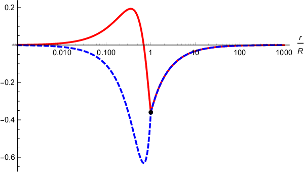
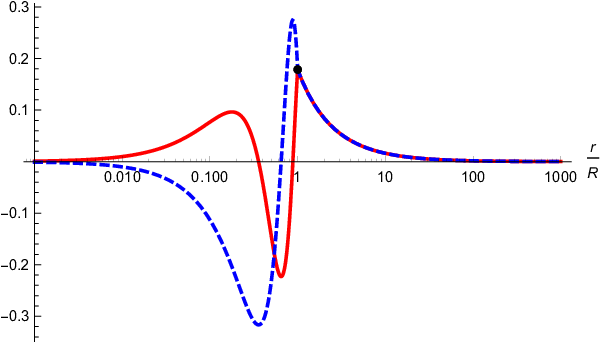
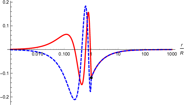
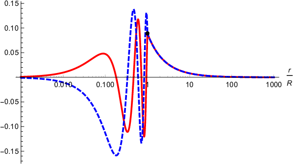
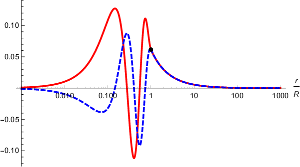
We then investigate numerical solutions satisfying the conditions Q1,in​(ℛ)=Q2,in​(ℛ)Q_{1,{\rm in}}(\mathcal{R})=Q_{2,{\rm in}}(\mathcal{R}) and Q3,in​(ℛ)=Q4,in​(ℛ)Q_{3,{\rm in}}(\mathcal{R})=Q_{4,{\rm in}}(\mathcal{R}). For this purpose, we introduce the dimensionless quantities β¯1:=c4​β1/(8​π​G​ℛ)\bar{\beta}_{1}:=c^{4}\beta_{1}/(8\pi G{\cal R}) and x:=r/ℛx:=r/\mathcal{R}, where x=1x=1 corresponds to the surface of the star. In Fig. 1, Q1Q_{1} and Q2Q_{2} are shown as the functions of xx for 𝒞=0.1{\cal C}=0.1. The top-left, top-right, bottom-left, and bottom-right panels correspond to the 0-, 1-, 2-, and 3-node solutions of Q2Q_{2} which are obtained for β¯1=11.32,22.95,34.50,46.04\bar{\beta}_{1}=11.32,22.95,34.50,46.04, respectively. The red and blue dashed curves correspond to Q1Q_{1} and Q2Q_{2}, respectively. The black points correspond to the surface of the star at x=1x=1.

Refer to caption
Refer to caption
Refer to caption
Refer to caption
Figure 1: Q1Q_{1} and Q2Q_{2} are shown as the functions of xx for 𝒞=0.1{\cal C}=0.1. The top-left, top-right, bottom-left, and bottom-right panels correspond to the 0-node, 1-node, 2-node, and 3-node solutions of Q2Q_{2} obtained for β¯1=11.32,22.95,34.50,46.04\bar{\beta}_{1}=11.32,22.95,34.50,46.04, respectively. The red and blue dashed curves correspond to Q1Q_{1} and Q2Q_{2}, respectively. The black points correspond to the surface of the star at x=1x=1. Q1Q_{1} always has one more node than Q2Q_{2}.

As β¯1\bar{\beta}_{1} increases, the solutions with more nodes are obtained. We note that Q1Q_{1} always has one more node than Q2Q_{2}. As expected, the first order derivatives Q1′​(x)Q_{1}^{\prime}(x) and Q2′​(x)Q_{2}^{\prime}(x) are discontinuous at the surface of the star x=1x=1 for any number of nodes. We note that since the equations are linear, if Q1Q_{1} and Q2Q_{2} are solutions, c′​Q1c^{\prime}Q_{1} and c′​Q2c^{\prime}Q_{2} with c′c^{\prime} being constant are also the solutions, and the solutions for Q3Q_{3} and Q4Q_{4} can be obtained by the relations Q3/Q1=Q4/Q2Q_{3}/Q_{1}=Q_{4}/Q_{2}, respectively.

We expect that the above lowest 00-node solution arises as the consequence of the tachyonic instability of the trivial solution ψ=0\psi=0. When we consider the small perturbations about the trivial solution ψ=0\psi=0, the zero frequency eigenstate of the perturbations cannot be the ground state for β¯1≥11.32{\bar{\beta}}_{1}\geq 11.32 and the end point of the tachyonic instability would be the nontrivial solutions constructed in this section.

IV.5 Coupling to the pressure

The problem of the discontinuity of the first order derivatives may be solved, for instance, if we consider the coupling only to the pressure

(γμ​Dμ+3​β22​γ^5​p~​(r))​ψ=0,\displaystyle\left({\gamma}^{\mu}D_{\mu}+\frac{3\beta_{2}}{2}{\hat{\gamma}}^{5}{\tilde{p}}(r)\right)\psi=0, (57)

where β2\beta_{2} is the coupling constant. Since the pressure p~​(r){\tilde{p}}(r) vanishes at the surface of the star r=ℛr=\mathcal{R}, the first order derivative of ψ\psi with respect to rr as well as ψ\psi itself is continuous there. Introducing the dimensionless quantity β¯2:=c4​β2/(8​π​G​ℛ)\bar{\beta}_{2}:=c^{4}\beta_{2}/(8\pi G{\cal R}), in Fig. 2, we show an example of Q1Q_{1} and Q2Q_{2} as the functions of x=r/ℛx=r/\mathcal{R} for 𝒞=0.1{\cal C}=0.1. The top-left, top-right, bottom-left, and bottom-right panels correspond to the 0-, 1-, 2-, and 3-node solutions of Q1Q_{1} obtained for β¯2=89.05,168.82,249.66,330.88\bar{\beta}_{2}=89.05,168.82,249.66,330.88, respectively. The red and blue dashed curves correspond to Q1Q_{1} and Q2Q_{2}, respectively. The black points correspond to the surface of the star.

Refer to caption
Refer to caption
Refer to caption
Refer to caption
Figure 2: Q1Q_{1} and Q2Q_{2} are shown as the functions of x=r/ℛx=r/\mathcal{R} for 𝒞=0.1{\cal C}=0.1. The top-left, top-right, bottom-left, and bottom-right panels correspond to the 0-, 1-, 2-, and 3-node solutions of Q1Q_{1} obtained for β¯2=89.05,168.82,249.66,330.88\bar{\beta}_{2}=89.05,168.82,249.66,330.88, respectively. The red and blue dashed curves correspond to Q1Q_{1} and Q2Q_{2}, respectively. The black points correspond to the surface of the star. Q2Q_{2} always has one more node than Q1Q_{1}.

Q2Q_{2} always has one more node than Q1Q_{1}. We note that as in the previous case the solution for Q3Q_{3} and Q4Q_{4} can be obtained with the relation Q3/Q1=Q4/Q2Q_{3}/Q_{1}=Q_{4}/Q_{2}, respectively.

We confirmed that the solutions for the Dirac spinor field and their first order derivatives for any number of nodes are continuous across the surface of the star x=1x=1, i.e., r=ℛr=\mathcal{R}. Thus, any component of the effective energy-momentum tensor is continuous across the surface of the star, even if it takes a nonzero value. However, since Eq. (57) is not derived from the variation of the action and is more specific to the observer who is at rest at the spatial infinity, the above argument seems to depend on the choice of the coordinates. Further studies on the possible improved couplings would be left for future work.

V Stealth spontaneous spinorization

One might imagine that the discontinuity of the first order derivative of Q1Q_{1}, Q2Q_{2}, Q3Q_{3}, and Q4Q_{4} at the surface of the star x=1x=1, r=ℛr=\mathcal{R} would result in the discontinuity in the effective energy density and pressure of the Dirac spinor field. If it is the case, there should be the localized source of the Dirac spinor field at the surface of the star, whose existence seems to be unphysical. We again emphasize that the discontinuity is somewhat an artifact of the idealization of the background solutions, and since in realistic relativistic stellar backgrounds the matter energy density would quickly but smoothly go to zero, the discontinuity of ∂rψ\partial_{r}\psi would also be smoothened. In addition, in this section, we argue that even in the original model the existence of the discontinuity does not matter, as all the components of the effective energy-momentum tensor of the Dirac field trivially vanish in any spherically symmetric backgrounds.

We now define the effective energy-momentum tensor for the Dirac field from Eqs. (11) and (15), which up to the quadratic order of ψ\psi and ψ¯{\bar{\psi}} is given by

Tμ​ν(ψ,eff)\displaystyle T^{(\psi,{\rm eff})}_{\mu\nu} :⁣=\displaystyle:= −12∑I=1,2[ψ¯Iγ^5eb⁡(μCLOSEγ^bDOPENν)ψI−(D(μCLOSEψ¯I)γ^5γ^beOPENb|ν)ψI]+β1Tμ​ν(m)∑I=1,2ψ¯IψI+𝒪(ψ4),\displaystyle-\frac{1}{2}\sum_{I=1,2}\left[{\bar{\psi}}_{I}{\hat{\gamma}}^{5}e_{b(\mu}{\hat{\gamma}}^{b}D_{\nu)}\psi_{I}-\left(D_{(\mu}{\bar{\psi}}_{I}\right){\hat{\gamma}}^{5}{\hat{\gamma}}^{b}e_{b|\nu)}\psi_{I}\right]+\beta_{1}{T}^{(m)}_{\mu\nu}\sum_{I=1,2}{\bar{\psi}}_{I}\psi_{I}+{\cal O}(\psi^{4}), (58)

where 𝒪⁡(ψ4){\cal O}(\psi^{4}) denotes all the quartic order combinations of ψI\psi_{I}, ψ¯I{\bar{\psi}}_{I} and their first order derivatives. Following the arguments in Sec. III.2, it is straightforward to confirm that for any two Dirac spinor fields that maintain the spherical symmetry of the spacetime

ψ1=h⁡(t)​ei​ϕ2r​eν/4​(cos⁡(θ2)​[(1+i)​f​(r)+(1−i)​g​(r)]i​sin⁡(θ2)​[(1−i)​f​(r)+(1+i)​g​(r)]cos⁡(θ2)​[(1−i)​f​(r)+(1+i)​g​(r)]−i​sin⁡(θ2)​[(1+i)​f​(r)+(1−i)​g​(r)]),\displaystyle\psi_{1}=\frac{h(t)e^{i\frac{\phi}{2}}}{re^{\nu/4}}\begin{pmatrix}\cos\left(\frac{\theta}{2}\right)\left[(1+i)f(r)+(1-i)g(r)\right]\\ i\sin\left(\frac{\theta}{2}\right)\left[(1-i)f(r)+(1+i)g(r)\right]\\ \cos\left(\frac{\theta}{2}\right)\left[(1-i)f(r)+(1+i)g(r)\right]\\ -i\sin\left(\frac{\theta}{2}\right)\left[(1+i)f(r)+(1-i)g(r)\right]\end{pmatrix}, (59)

and

ψ2=h⁡(t)​e−i​ϕ2r​eν/4​(i​sin⁡(θ2)​[(1+i)​f​(r)+(1−i)​g​(r)]cos⁡(θ2)​[(1−i)​f​(r)+(1+i)​g​(r)]i​sin⁡(θ2)​[(1−i)​f​(r)+(1+i)​g​(r)]−cos⁡(θ2)​[(1+i)​f​(r)+(1−i)​g​(r)]),\displaystyle\psi_{2}=\frac{h(t)e^{-i\frac{\phi}{2}}}{re^{\nu/4}}\begin{pmatrix}i\sin\left(\frac{\theta}{2}\right)\left[(1+i)f(r)+(1-i)g(r)\right]\\ \cos\left(\frac{\theta}{2}\right)\left[(1-i)f(r)+(1+i)g(r)\right]\\ i\sin\left(\frac{\theta}{2}\right)\left[(1-i)f(r)+(1+i)g(r)\right]\\ -\cos\left(\frac{\theta}{2}\right)\left[(1+i)f(r)+(1-i)g(r)\right]\end{pmatrix}, (60)

where h⁡(t)h(t) is any complex function of time tt, all the components of Tμ​ν(ψ,eff)T^{(\psi,{\rm eff})}_{\mu\nu} vanish both inside and outside the star at least at 𝒪⁡(ψ2){\cal O}(\psi^{2}). The limits to the surface of the star from the inside (r→ℛ−0r\to{\cal R}_{-0}) and that from the outside (r→ℛ+0r\to{\cal R}_{+0}) converge to the unique value 00. Thus, all components of the effective energy-momentum tensor for the Dirac spinor vanish in the entire spacetime at least at 𝒪⁡(ψ2){\cal O}(\psi^{2}). This indicates that the tachyonic growth of the Dirac spinor field does not backreact on the spacetime geometry, and the metric solution remains the same as in general relativity. The tachyonic growth would be quenched by the nonlinear effects in the effective Dirac field equation (17) as in the case of spontaneous scalarization Minamitsuji and Ikeda 2019; Silva et al. 2019. As argued in Sec. III.3, since ρ(ψ2)=−ρ(ψ1)\rho_{(\psi_{2})}=-\rho_{(\psi_{1})}, one of the two Dirac fields has the positive energy density, while the other has the negative one. However, the negative energy density of one field does not imply any pathology, as only the combination of the two Dirac fields has the physical meaning to maintain the static and spherically symmetric spacetime. Since Φ=∑Iψ¯I​ψI=0\Phi=\sum_{I}{\bar{\psi}}_{I}\psi_{I}=0, F=1F=1 in Eq. (15) and hence there is no distinction between the Jordan and Einstein frames. After all, we expect that spontaneous spinorization proceeds as a stealth process and does not leave any observable effects. Thus, we call this stealth spinorization.

Since the property of the vanishing effective energy-momentum tensor holds in any static and spherically symmetric spacetime, we conclude that the above stealth spinorization will happen in any static and spherically symmetric general relativistic stellar backgrounds with more realistic equations of state. As the next step, it is of interest whether the conclusion remains the same in less symmetric general relativistic stellar backgrounds, such as stationary and axisymmetric spacetimes around rotating stars. Moreover, since our model introduced in Sec. II corresponds to the simplest model for spontaneous spinorization, it is also of interest to explore more general models Ramazano˘glu 2018.

VI Conclusions

We have investigated the possibility of the tachyonic growth of the Dirac spinor field ψ\psi on general relativistic stellar backgrounds and spontaneous spinorization of compact objects, which is analogous to spontaneous scalarization studied in many previous works. We have focused on the theory (8) and (9), which is composed of the modified kinetic term by the insertion of the fifth gamma matrix γ^5{\hat{\gamma}}^{5} and the conformal coupling of the Dirac spinor field to matter and would lead to the tachyonic growth of the Dirac spinor field only in the high density backgrounds. At the linearized level, the Dirac equation (7) is very similar to the tachyonic Dirac spinor field theory (4), where the mass parameter MM is replaced by the trace of the matter energy-momentum tensor T(m)​μμT^{(m)\mu}{}_{\mu}.

As in the case of spontaneous scalarization, we naively expect that the tachyonic growth of the Dirac spinor field would significantly modify the structure of relativistic stars from general relativistic ones. In order to obtain the spherically symmetric solutions, we have to consider the two Dirac fields at the same time such as Eqs. (43) and (44). We have confirmed that at the linearized equation for ψ\psi our theory gives rise to the nontrivial profiles of the Dirac spinor field with any number of nodes and the vanishing field values at the spatial infinity. However, we have also confirmed that all the components of the effective energy-momentum tensor of the Dirac spinor fields vanish up to the quadratic order of ψ\psi and ψ¯{\bar{\psi}} in the entire spacetime including the surface of the star, when the contributions of both the two Dirac spinor fields are taken into consideration. Thus, we have expected that spontaneous spinorization proceeds as a stealth process unlike spontaneous scalarization, and hence does not leave any observable effects.

The status of the study of spontaneous spinorization is still immature, and several issues should be clarified in future work. Although we have focused on the static and spherically symmetric stars, it would be important to clarify whether this stealth property holds in less symmetric backgrounds such as rotating and binary stars. It would also be necessary to follow the time evolution from general relativistic stellar solutions to those with nontrivial profile of the Dirac spinor fields. Another direction of the study is to generalize the model considered in this paper and explore novel features of spontaneous spinorization. We hope to come back to these issues in our future work.

Acknowledgements.
M.M. was supported by the Portuguese national fund through the Fundação para a Ciência e a Tecnologia within the framework of the Decree-Law 57/2016 of August 29 (changed by Law 57/2017 of July 19), and the CENTRA through the Project No. UIDB/00099/2020.

Appendix A Consistent action for the Dirac spinor field in the flat and curved spacetimes

A.1 In the Minkowski spacetime

In this appendix, we review the consistency of the equation of motion for the Dirac adjoint ψ¯\bar{\psi} in the tachyonic Dirac field theory. Varying the actions (4) and (6) with respect to ψ¯\bar{\psi} and ψ\psi, we obtain the following equations, respectively:

(γ^5γ^a∂a−M)ψ=0,ψ¯(∂←aγ^5γ^a+M)=0,\displaystyle\left({\hat{\gamma}}^{5}{\hat{\gamma}}^{a}\partial_{a}-M\right)\psi=0,\qquad{\bar{\psi}}\left(\overleftarrow{\partial}_{a}{\hat{\gamma}}^{5}{\hat{\gamma}}^{a}+M\right)=0, (61)

and

(γ^5γ^a∂a−M)ψ=0,ψ¯(∂←aγ^aγ^5+M)=0.\displaystyle\left({\hat{\gamma}}^{5}{\hat{\gamma}}^{a}\partial_{a}-M\right)\psi=0,\qquad{\bar{\psi}}\left(\overleftarrow{\partial}_{a}{\hat{\gamma}}^{a}{\hat{\gamma}}^{5}+M\right)=0. (62)

Since {γ^5,γ^a}=0\{{\hat{\gamma}}^{5},{\hat{\gamma}}^{a}\}=0, we obtain the different results in the equations for ψ¯\bar{\psi}, and see which one is consistent. Taking the conjugate transpose of the equation for ψ\psi,

0\displaystyle 0 =\displaystyle= ψ†​(∂←a​(γ^a)†​γ^5−M)=ψ†​(−∂←a​γ^5​(γ^a)†−M)\displaystyle{\psi}^{\dagger}\left(\overleftarrow{\partial}_{a}\left({\hat{\gamma}}^{a}\right)^{\dagger}{\hat{\gamma}}^{5}-M\right)={\psi}^{\dagger}\left(-\overleftarrow{\partial}_{a}{\hat{\gamma}}^{5}\left({\hat{\gamma}}^{a}\right)^{\dagger}-M\right) (63)
=\displaystyle= ψ†​(−∂←0​γ^5​(γ^0)†−∂←i​γ^5​(γ^i)†−M)=ψ†​(−∂←0​γ^0​γ^5+∂←i​γ^i​γ^5−M),\displaystyle{\psi}^{\dagger}\left(-\overleftarrow{\partial}_{0}{\hat{\gamma}}^{5}\left({\hat{\gamma}}^{0}\right)^{\dagger}-\overleftarrow{\partial}_{i}{\hat{\gamma}}^{5}\left({\hat{\gamma}}^{i}\right)^{\dagger}-M\right)={\psi}^{\dagger}\left(-\overleftarrow{\partial}_{0}{\hat{\gamma}}^{0}{\hat{\gamma}}^{5}+\overleftarrow{\partial}_{i}{\hat{\gamma}}^{i}{\hat{\gamma}}^{5}-M\right),

where the index i=1,2,3i=1,2,3 represent the spatial directions and we have employed (γ^5)†=γ^5({\hat{\gamma}}^{5})^{\dagger}={\hat{\gamma}}^{5}, γ^5​(γ^0)†−γ^0​γ^5=0{\hat{\gamma}}^{5}({\hat{\gamma}}^{0})^{\dagger}-{\hat{\gamma}}^{0}{\hat{\gamma}}^{5}=0, and γ^5​(γ^i)†+γ^i​γ^5=0{\hat{\gamma}}^{5}({\hat{\gamma}}^{i})^{\dagger}+{\hat{\gamma}}^{i}{\hat{\gamma}}^{5}=0. Multiplying −i​γ^0-i{\hat{\gamma}}^{0} from the right side,

0\displaystyle 0 =\displaystyle= −i​ψ†​(−∂←0​γ^0​γ^5+∂←i​γ^i​γ^5−M)​γ^0=−i​ψ†​(−∂←0​γ^0​γ^5+∂←i​γ^i​γ^5)​γ^0−M​ψ¯\displaystyle-i{\psi}^{\dagger}\left(-\overleftarrow{\partial}_{0}{\hat{\gamma}}^{0}{\hat{\gamma}}^{5}+\overleftarrow{\partial}_{i}{\hat{\gamma}}^{i}{\hat{\gamma}}^{5}-M\right){\hat{\gamma}}^{0}=-i{\psi}^{\dagger}\left(-\overleftarrow{\partial}_{0}{\hat{\gamma}}^{0}{\hat{\gamma}}^{5}+\overleftarrow{\partial}_{i}{\hat{\gamma}}^{i}{\hat{\gamma}}^{5}\right){\hat{\gamma}}^{0}-M{\bar{\psi}} (64)
=\displaystyle= −i​ψ†​(∂←0​γ^0​γ^0​γ^5+∂←i​γ^0​γ^i​γ^5)−M​ψ¯=ψ¯​(∂←0​γ^0​γ^5+∂←i​γ^i​γ^5)−M​ψ¯\displaystyle-i{\psi}^{\dagger}\left(\overleftarrow{\partial}_{0}{\hat{\gamma}}^{0}{\hat{\gamma}}^{0}{\hat{\gamma}}^{5}+\overleftarrow{\partial}_{i}{\hat{\gamma}}^{0}{\hat{\gamma}}^{i}{\hat{\gamma}}^{5}\right)-M{\bar{\psi}}={\bar{\psi}}\left(\overleftarrow{\partial}_{0}{\hat{\gamma}}^{0}{\hat{\gamma}}^{5}+\overleftarrow{\partial}_{i}{\hat{\gamma}}^{i}{\hat{\gamma}}^{5}\right)-M{\bar{\psi}}
=\displaystyle= ψ¯​(∂←a​γ^a​γ^5−M)=−ψ¯​(∂←a​γ^5​γ^a+M),\displaystyle{\bar{\psi}}\left(\overleftarrow{\partial}_{a}{\hat{\gamma}}^{a}{\hat{\gamma}}^{5}-M\right)=-{\bar{\psi}}\left(\overleftarrow{\partial}_{a}{\hat{\gamma}}^{5}{\hat{\gamma}}^{a}+M\right),

which reproduces the equation for ψ¯{\bar{\psi}} in Eq. (61). Thus, the action (4) provides the consistent equation of motion for ψ¯\bar{\psi} Jentschura and Wundt 2012; Ramazano˘glu 2018.

A.2 In the curved spacetimes

The extension to the case of the curved spacetime is also straightforward. Varying the action of the tachyonic Dirac field (30) in the curved spacetime with respect to ψ¯\bar{\psi} and ψ\psi, respectively we obtain the following equations:

(γ^5γμ(∂μ+Γμ)−M)ψ=0,ψ¯((∂←μ−Γμ)γ^5γμ+M)=0.\displaystyle\left({\hat{\gamma}}^{5}{\gamma}^{\mu}\left(\partial_{\mu}+\Gamma_{\mu}\right)-M\right)\psi=0,\qquad{\bar{\psi}}\left(\left(\overleftarrow{\partial}_{\mu}-\Gamma_{\mu}\right){\hat{\gamma}}^{5}{\gamma}^{\mu}+M\right)=0. (65)

Taking the conjugate transpose to the equation for ψ\psi,

0\displaystyle 0 =\displaystyle= ψ†​((∂←μ+(Γμ)†)​(γμ)†​γ^5−M)=ψ†​((∂←t+(Γt)†)​(γt)†​γ^5+(∂←k+(Γk)†)​(γk)†​γ^5−M)\displaystyle{\psi}^{\dagger}\left(\left(\overleftarrow{\partial}_{\mu}+(\Gamma_{\mu})^{\dagger}\right)\left({\gamma}^{\mu}\right)^{\dagger}{\hat{\gamma}}^{5}-M\right)={\psi}^{\dagger}\left(\left(\overleftarrow{\partial}_{t}+(\Gamma_{t})^{\dagger}\right)\left({\gamma}^{t}\right)^{\dagger}{\hat{\gamma}}^{5}+\left(\overleftarrow{\partial}_{k}+(\Gamma_{k})^{\dagger}\right)\left({\gamma}^{k}\right)^{\dagger}{\hat{\gamma}}^{5}-M\right) (66)
=\displaystyle= ψ†​(−(∂←t+(Γt)†)​γt​γ^5+(∂←k+(Γk)†)​γk​γ^5−M),\displaystyle{\psi}^{\dagger}\left(-\left(\overleftarrow{\partial}_{t}+(\Gamma_{t})^{\dagger}\right){\gamma}^{t}{\hat{\gamma}}^{5}+\left(\overleftarrow{\partial}_{k}+(\Gamma_{k})^{\dagger}\right){\gamma}^{k}{\hat{\gamma}}^{5}-M\right),

where kk denotes the spatial indices and we have employed the relations of the gamma matrices (γ^5)†=γ^5({\hat{\gamma}}^{5})^{\dagger}={\hat{\gamma}}^{5}, γt+(γt)†=0\gamma^{t}+\left(\gamma^{t}\right)^{\dagger}=0, and γk−(γk)†=0\gamma^{k}-\left(\gamma^{k}\right)^{\dagger}=0. Multiplying −i​γ^0-i{\hat{\gamma}}^{0} from the right side,

0\displaystyle 0 =\displaystyle= −i​ψ†​(−(∂←t+(Γt)†)​γt​γ^5+(∂←k+(Γk)†)​γk​γ^5−M)​γ^0\displaystyle-i{\psi}^{\dagger}\left(-\left(\overleftarrow{\partial}_{t}+(\Gamma_{t})^{\dagger}\right){\gamma}^{t}{\hat{\gamma}}^{5}+\left(\overleftarrow{\partial}_{k}+(\Gamma_{k})^{\dagger}\right){\gamma}^{k}{\hat{\gamma}}^{5}-M\right){\hat{\gamma}}^{0} (67)
=\displaystyle= −i​ψ†​((∂←t+(Γt)†)​γ^0​γt​γ^5+(∂←k+(Γk)†)​γ^0​γk​γ^5−M​γ^0)\displaystyle-i{\psi}^{\dagger}\left(\left(\overleftarrow{\partial}_{t}+(\Gamma_{t})^{\dagger}\right){\hat{\gamma}}^{0}{\gamma}^{t}{\hat{\gamma}}^{5}+\left(\overleftarrow{\partial}_{k}+(\Gamma_{k})^{\dagger}\right){\hat{\gamma}}^{0}{\gamma}^{k}{\hat{\gamma}}^{5}-M{\hat{\gamma}}^{0}\right)
=\displaystyle= ψ¯​((∂←t−Γt)​γt​γ^5+(∂←k−Γk)​γk​γ^5−M)=ψ¯​((∂←μ−Γμ)​γμ​γ^5−M)\displaystyle{\bar{\psi}}\left(\left(\overleftarrow{\partial}_{t}-\Gamma_{t}\right){\gamma}^{t}{\hat{\gamma}}^{5}+\left(\overleftarrow{\partial}_{k}-\Gamma_{k}\right){\gamma}^{k}{\hat{\gamma}}^{5}-M\right)={\bar{\psi}}\left(\left(\overleftarrow{\partial}_{\mu}-\Gamma_{\mu}\right){\gamma}^{\mu}{\hat{\gamma}}^{5}-M\right)
=\displaystyle= −ψ¯​((∂←μ−Γμ)​γ^5​γμ+M),\displaystyle-{\bar{\psi}}\left(\left(\overleftarrow{\partial}_{\mu}-\Gamma_{\mu}\right){\hat{\gamma}}^{5}{\gamma}^{\mu}+M\right),

where we have used γ^0​Γμ+(Γμ)†​γ^0=0{\hat{\gamma}}^{0}\Gamma_{\mu}+\left(\Gamma_{\mu}\right)^{\dagger}{\hat{\gamma}}^{0}=0, which reproduces the equation for ψ¯{\bar{\psi}} in Eq. (65). Thus, the action (30) provides the consistent equation of motion for ψ¯\bar{\psi}.

References