Keywords: Localization, Disordered systems, Non-equilibrium dynamics, Entanglement
Loschmidt echo singularities as dynamical signatures of strongly localized phasesJournal: New J. Phys.
Abstract
Quantum localization (single-body or many-body) comes with the emergence of local conserved quantities — whose conservation is precisely at the heart of the absence of transport through the system. In the case of fermionic systems and spin models, such conserved quantities take the form of effective two-level systems, called -bits. While their existence is the defining feature of localized phases, their direct experimental observation remains elusive. Here we show that strongly localized -bits bear a dramatic universal signature, accessible to state-of-the-art quantum simulators, in the form of periodic cusp singularities in the Loschmidt echo following a quantum quench from a Néel/charge-density-wave state. Such singularities are perfectly captured by a simple model of Rabi oscillations of an ensemble of independent two-level systems, which also reproduces the short-time behavior of the entanglement entropy and the imbalance dynamics. In the case of interacting localized phases, the dynamics at longer times shows a sharp crossover to a faster decay of the Loschmidt echo singularities, offering an experimentally accessible signature of the interactions between -bits.
1 Introduction
Constructive interference of paths bringing a particle back to its initial location in real space is at the heart of single-particle (or Anderson) localization (AL)[1, 2]; more recently a similar phenomenon occurring in Hilbert space (MBL) [3, 4, 5, 6] has been shown to prevent many-body quantum systems from relaxing to thermal equilibrium, undermining the ergodic hypothesis in a large class of models of interacting quantum particles. Localized phases are generally characterized in the negative (absence of transport, of long-range order, of spectral gaps, etc.), while positive characterizations are typically elusive. A crucial aspect of localization is the persistence of initial conditions, which, in the case of AL of non-interacting particles, is related to the conservation of populations in the localized single-particle eigenstates of the Hamiltonian. In the case of MBL, the analog phenomenon would be the appearance of local conserved quantities (called local integrals of motion or -bits [7, 8, 9, 10]) which are obtained by unitary transformations of local operators; and which, if extensive in number, constrain the dynamics of the system to the point of preventing relaxation.
The existence of -bits in disordered spin chains can be mathematically proven under the assumption of limited level attraction [9], and approximate -bits for many-body systems can be constructed with a variety of analytical as well as numerical methods [11, 12, 13, 14, 15, 16, 17, 18, 19, 20]. Much of the phenomenology of MBL dynamics (persistence of traits of the initial state, logarithmic growth of entanglement entropies, etc.) – observed in numerical studies as well as in experiments [4, 5] – can be directly explained in terms of the existence of -bits and interactions between them. Yet observing -bits directly is an arduous task, given that their expression is highly disorder-dependent (and generally unknown even in theory), and it would require high-precision measurements of local observables in different local bases. An even more ambitious task for experiments is the one of probing directly the existence of interactions among -bits, which is a defining feature distinguishing MBL from AL. Measuring the consequences of such interactions on correlation and entanglement dynamics is currently the focus of a considerable experimental effort based on state-of-the-art quantum simulation platforms [21, 22, 23].
The purpose of this work is to show that, in the case of strongly localized phases, the existence of -bits can offer striking signatures in the dynamics of the Loschmidt echo, namely in the logarithm of the return probability to the initial state
| (1) |
Here is the system’s Hamiltonian and the lattice size; indicates the disorder average. Please note that we employ the “Loschmidt echo” terminology similar to other recent works in which singular behavior has been observed in the quench dynamics of many-body quantum systems [24, 25, 26, 27, 28, 29, 30, 31]. Nonetheless, In the quantum-chaos literature the Loschmidt echo is more generally defined as the scalar product between the evolution of the same state with two different Hamiltonians, and [32, 33]. Starting from , our definition is retrieved in the case of and . When has a simple factorized form, and in the case of strong disorder, we find that the Loschmidt echo displays periodic singularities, decaying very slowly in amplitude – as illustrated using a model of disordered spinless fermions in 1d (corresponding to the XXZ model in a fully random or quasi-periodic field) initialized in a charge density-wave (CDW) state. The singularities in the Loschmidt echo are fully explained quantitatively by a simple model of a collection of localized 2-level systems (2LS) undergoing independent Rabi oscillations, and approximating strongly localized -bits. The same minimal model captures quantitatively the dynamics of the entanglement entropy at short times as well as of the number entropy at longer times; and the dynamics of the density imbalance characterizing the initial state.
At longer times the deviation of the exact results for the MBL dynamics from the predictions of the 2LS ensemble offers direct evidence of the interactions among the -bits in the form of a faster decay of the Loschmidt-echo singularities and imbalance oscillations. As the Loschmidt echo and the imbalance are generally accessible to quantum simulators, either measuring individual degrees of freedom [34, 26] or even global ones [35, 36, 37], our results show that strong direct signatures of -bits dynamics and interactions are within the immediate reach of state-of-the-art experiments on disordered quantum systems.
The structure of the paper is as follows: section 2 introduces the XXZ model in a random/quasi-periodic field; section 3 discusses the observation of Loschmidt echo singularities in the exact dynamics, as well as their quantitative understanding via a model of 2LS as well as three-level systems (3LS); section 5 discusses the dynamics of imbalance, and the comparison with the prediction of the 2LS and 3LS model; section 6 discusses the departure of the exact data (for the Loschmidt echo and imbalance dynamics) from the 2LS/3LS predictions as a signature of -bit interactions; section 7 shows that the 2LS/3LS models capture quantitatively the entanglement dynamics at short time, and of number entropy at longer times; conclusions are drawn in section 8.
2 Model
Our platform for the investigation of Loschmidt-echo dynamics is given by a paradigmatic model, namely the XXZ chain in an inhomogeneous magnetic field [38, 39], corresponding to a model of spinless fermions with nearest-neighbor interactions in an inhomogeneous local chemical potential [40]
where () are spin operators and and are fermionic operators; the equality between the two Hamiltonians is true up to an additive constant via Jordan-Wigner mapping. In the following the external field/potential is taken to be either quasi-periodic (QP) [41, 42], namely with (inspired by experiments on bichromatic optical lattices [35, 43]) and a random phase; or to be fully random (FR) and uniformly distributed in the interval . We consider chains of length (up to ) with open boundaries, and we average our results over realizations of the random phase (QP) or of the full random potential (FR). All the unitary evolutions considered in this study are obtained using exact diagonalization (ED), and they start from the charge-density wave state , corresponding to a Néel state for the spins. We shall focus on the case of interacting fermions (corresponding to an SU(2) invariant spin-spin interaction) and contrast it with the limit of free fermions . In the latter case, the QP potential leads to a transition to fully localized single-particle eigenstates for , with an energy independent localization length ; while the FR potential leads to AL of the whole spectrum at any infinitesimal value of disorder. In the interacting case, instead, a QP potential of strength [44] and a FR potential of strength [45, 46, 47, 48, 49, 50, 51, 52] are numerically found to lead to MBL. In the following sections we shall generally start our discussion from the case of the QP potential, which has a simpler spatial structure devoid of rare regions, leading to stronger localization effects; and we shall later discuss how to enrich the picture in the case of the FR potential, in order to account for the existence of rare regions.
3 Loschmidt echo singularities and imbalance oscillations
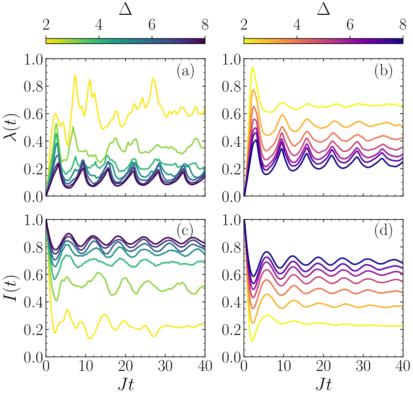
Figure 1 shows the dynamics of the Loschmidt echo , (1), along with that of the imbalance
| (2) |
The latter saturates to its maximum value of 1 in the initial state and probes the persistence of the initial density/spin pattern [35, 36, 37]. We observe that for both the QP and FR potentials, and for disorder strengths compatible with the onset of the MBL regime, the Loschmidt echo displays a sequence of periodic cusp-like peaks at times . These times correspond to minima in the imbalance, as the system reaches instantaneous configurations which are the farthest from the initial spin/density pattern.
A closer inspection shows that, for sufficiently strong disorder, all the peaks become sharp cusps, namely they represent genuine non-analyticities of the Loschmidt echo. They are rather remarkable given that they survive disorder averaging, and they seemingly appear in a finite fraction of disorder realizations (see C for further details); and in particular they decay very slowly in time, as we shall discuss in detail later on. The rest of this work will be devoted to developing a quantitative understanding of the dynamics of Loschmidt-echo singularities and imbalance oscillations as signatures of the existence of -bits and of their interacting nature.
4 Quantitative modeling of the Loschmidt echo singularities
4.1 Modeling with an ensemble of two-level systems
All the essential details of the short-time evolution of the Loschmidt echo can be captured with a surprisingly simple, yet rather insightful model. This model is best understood (and justified) in the case of the QP potential, as illustrated in figure 2.

In the case of strong disorder, the fastest dynamics in the system starting from a Fock state will be offered by those particles that sit on a site which is nearly resonant with its unoccupied neighbor (say ), because the hopping is either larger than the energy offset (in the non-interacting case) or larger than the screened offset (in the presence of nearest-neighbor repulsion). These 2-site clusters, representing nearly resonant two-level systems (2LS), have the property of being spatially isolated in the QP potential, because of the strong anticorrelation among two consecutive energy offsets ( and – see B). As a consequence, a nearly resonant 2-site system will be generally surrounded by highly non-resonant pairs of sites, which can be considered as nearly frozen to the initial state. This invites us to write for the evolved state a 2LS Ansatz
| (3) |
where the first tensor product runs over the nearly resonant 2LS, while the second tensor product runs over the leftover sites (we have taken the freedom of reordering the sites arbitrarily in the tensor product; see [53, 54, 55] for a similar Ansatz to study the long-time dynamics). is the evolved state of the -th (isolated) 2LS system, corresponding to two states split by an energy difference and connected by a Rabi coupling ; while is the (persistent) initial state of the site belonging to the remainder of the system. The Loschmidt echo for such a system is readily calculated as
| (4) |
with (and ) the well-known probability of finding the 2LS in the state orthogonal to the initial one while performing Rabi oscillations [56] – see also A. When averaging Eq. (4) over disorder, it is immediate to obtain the following simple expression
| (5) |
where is the probability that the energy offset between two neighboring sites takes the value . Going from Eq. (4) to Eq. (5) implies that we in fact count all of the pairs of sites in a chain as nearly resonant 2LS, thereby counting twice every site. The mistake that one makes in doing this is minor, though, because the non-resonant pairs of sites give a very small contribution to the Loschmidt echo; and, if neighboring pairs of sites are not simultaneously resonant, a site will not be counted twice in practice. Eq. (5) is an analytical integral formula which depends uniquely on the (known) statistics of the disorder potential via the distribution. In the case of the QP potential
| (6) |
with [57]; while for the FR potential is the normalized triangular distribution defined on the interval.
The cusp singularities in at times , , descend from the fact that the integrand function , seen as a function of , develops a logarithmic singularity at , as shown in figure 3, while it is fully regular at any other time. The singular peak centered at has a support shrinking with as – as seen in figure 3 when plotting the function vs , which leads to a collapse of the peak widths at different times (when ). The integral of the function outside the peak contributes to the regular part of the Loschmidt echo, while the integral of the peak dictates fundamentally the height of the cusps above the regular background (estimated as the long-time average ), namely the quantity . The decay of the height of these cusps as will be verified numerically in section 6. Figure 4(a-b) shows that, for the case of the QP potential, Eq. (5) is able to predict with high accuracy the ED results deep in the MBL phase without any adjustable parameter. In particular the cusp singularities of the ED results are easily explained as descending from the divergent singularity of the Loschmidt echo for a fully resonant 2LS with , reaching a state orthogonal to the initial one after odd multiples of half a Rabi oscillation . These divergences are smoothened into cusp singularities due to the fact that such resonant 2LSs are a set of zero measure in the disorder statistics. This result has important consequences. Indeed the nearly resonant 2LSs captured by the model are clearly an ensemble of approximate -bits with Hamiltonian
| (7) |
where is a Pauli matrix expressed as a rotation of the Pauli operators (when projected onto the subspace with ) and , built from the original spin operators for the pair ; and is the -bit splitting. Hence the Loschmidt-echo singularities are a striking manifestation of the existence of such (nearly free) -bits, to be found in the short-time dynamics of the system.
4.2 Relationship to dynamical quantum phase transitions
It is worthwhile to mention at this point that the existence of singularities in the quench dynamics of the Loschmidt echo is currently the subject of several theoretical and experimental investigations, as they represent the main signature of so-called dynamical quantum phase transitions, studied both in non-random systems [24, 25, 26, 30, 31] as well as in disordered quantum systems [27, 28, 58]. Nonetheless our observation of Loschmidt-echo singularities is fully explained by a model of individual 2LS, without the need of any many-body effect. Therefore we shall refrain from associating them to any form of time-dependent transition.
4.3 From two-level systems to three-level ones
Figure 4(d-f) shows that, in the case of the FR potential, the 2LS model of (5) still predicts the correct frequency of the Loschmidt echo singularities, but not the correct height; and it also misses a global offset. This is not surprising, as in the case of the FR potential the assumption of anti-correlation between the energy offset of contiguous pairs is no longer valid, namely the potential can host “rare” regions in which contiguous pairs of sites – and – are nearly resonant at the same time. To take those regions into account (at least partially) one can easily promote the 2LS model to a model of 3-site systems (amounting to effective three-level systems – 3LS), and approximate the evolved state as that of a collection of independent 3LS. The Hamiltonian of a three-site system containing two interacting fermions in an initial state is explicitly given by
| (8) |
Here all single-site energies are referred to the energy of site , and . The above Hamiltonian assumes that the sites and remain empty during the time evolution. The Hilbert space of the 3-site system is restricted to the three states , and , making of it a three-level system (3LS), with a generic time-dependent wavefunction
| (9) |
Its explicit form can be easily calculated numerically for any specific choice of the energy differences .
A similar calculation can be done for a three-site system hosting a single particle, and starting from the configuration, with Hamiltonian
| (10) |
which assumes that the sites and host two pinned particles. The Hilbert space , , defines a 3LS, whose instantaneous state takes the generic form
| (11) |
For the two types of clusters the Loschmidt echo can be readily evaluated as and .
We can then model a chain in a QP or FR potential as an ensemble of independent 3LSs by generating sequences of energy offsets between adjacent site pairs according to the distribution . The 3LS prediction for the Loschmidt echo of the ensemble is
| (12) |
In practice, the above integral can be sampled numerically by simply averaging over a large number of different realizations of the potential on 3-site systems, such as those offered by a very long chain, namely
| (13) |
where if is odd and if is even, and .
Eq. (13) for the Loschmidt echo has the apparent drawback of triple-counting each site. Nonetheless, similarly to what was argued for the 2LS case, it is fair to assume (and it can be numerically tested) that, out of the three clusters containing each site, only one at most will contribute significantly to the Loschmidt echo. As a consequence the triple counting has only a mild effect on the final result. One could avoid triple counting by thoughtfully decomposing a chain into non-overlapping clusters of up to 3 sites, in such a way as to maximize the Loschmidt echo; yet this procedure introduces significant complications which are not justified a posteriori, given the quality of the results offered already by the naive ensemble average. As shown by figure 4(c-d), the improvement offered by the 3LS model for the FR potential is substantial; these results can further be improved by moving to 4-site clusters etc., albeit at an exponential cost.
5 Imbalance dynamics
The 2LS model prediction for the imbalance is very similar to that of the Loschmidt echo, as the imbalance is simply related to the persistence probability of the initial state ( or ) on the 2-site cluster – given that the orthogonal state contributes zero to the imbalance. Therefore the 2LS expression for the imbalance simply reads
| (14) |
The times giving cusp singularities in the Loschmidt echo correspond to dips in the imbalance, and these dips come from local dips in the function centered around and touching zero for . The width of these dips is also shrinking in time as . Therefore one expects the depth of the minima in the fluctuations of the imbalance to decay to the long-time average as as well – this prediction will be verified in section 6.
Extending the 2LS model to 3LS, the imbalance can be calculated as
| (15) |
with or depending on whether is odd or even. Figure 5 shows the comparison between the ED results for the imbalance dynamics of interacting fermions immersed in a QP and fully random potentials of variable strength, compared with the predictions of the 2LS and the 3LS models. For sufficiently strong disorder () the 2LS predictions are already rather accurate in the case of the QP potential, and the 3LS model offers further improvement. On the other hand in the case of the FR potential the 3LS model offers a more substantial improvement, fixing an overall offset (for sufficiently strong disorder) which is seen in the 2LS predictions.
6 Dephasing in the Loschmidt echo and imbalance oscillations: evidence of -bits interactions
A significant feature of the Loschmidt echo singularities is their slow decay in time – which is remarkable given that they result from the Rabi oscillations of a collection of 2LS with a distribution of frequencies that can be a priori expected to lead to fast dephasing. The reason behind the slow decay is also captured by the 2LS model, Eq. (5) – namely by the fact that the integral expressing the Loschmidt echo takes contributions from a small window of detunings around zero, the smaller the longer the time, as mentioned in section 4.1. When looking at the singularity times , a direct inspection of the function seen as a function of shows that it has a large peak centered on with a width depending on time as . The singularity in the average Loschmidt echo comes from the integral of this peak, while the rest of the integral contributes essentially to the regular part of the Loschmidt echo; hence it is immediate to predict that the height of the cusp singularity should decay as the peak width, (namely as ).
Figure 6(a) shows the time evolution of singularity peaks in the Loschmidt echo for free as well as interacting fermions in the QP potential, compared to the prediction of the 2LS model (for the interacting case): we observe that the decay is indeed confirmed by the ED data for free fermions, as well as by the ED data for interacting fermions at sufficiently short times ( for ). On the other hand, at longer times the interacting data are found to display a strong deviation from the 2LS model prediction, exhibiting a much faster decay. This crossover to an interaction-induced dephasing (IID) regime clearly shows the limits of the 2LS model as a model of free -bits, and it marks a fundamental difference between AL and MBL in the QP system. Indeed the faster decay of the Loschmidt echo must be related to the effect of -bit interactions, which are a defining feature of MBL, and which add terms of the kind
| (16) |
to the effective -bit Hamiltonian (7). Such terms are responsible for the persistent growth of entanglement entropy in the system [7] as the logarithm of time, and indeed the onset of the growth of entanglement occurs at a time compatible with (see section 7 - figure 7). A similar crossover from a slow power-law decay of the Loschmidt-echo peak height to a faster decay, dictated by the presence of interactions, is also exhibited by the comparison between the ED data for interacting fermions in the FR potential with the same data for non-interacting fermions and for the 3LS model – as shown in figure 6(b).
Remarkably, the same crossover between the dynamics of effectively independent -bits to a regime of interacting ones is observed in the decay of imbalance oscillations. Figure 6(c) shows the evolution of the depth of the minima of the imbalance at times , taken with respect to the long-time average, namely the quantity . We observe that the predictions of the 2LS system for the fermionic chain immersed in the QP potential shows a clear, slow power-law decay at long times, compatible with , which is indeed reproduced in the case of non-interacting fermions. In the case of interacting fermions, on the other hand, a crossover is observed at long times () to a faster decay, marking the IID regime. A similar picture is offered by the case of the FR potential. There the ED results are compared with the predictions from the 3LS model; the latter model predicts correctly the decay of the minima depth in the non-interacting case at all times, while the exact results for the interacting system show a clear crossover towards a faster decay for times . For both kinds of disorder, the crossover time is compatible both with what is observed in the decay of the Loschmidt echo as well as with the evolution of the entanglement entropy (see again figure 7 in the next section). Therefore we conclude that the crossover to the IID regime is a robust feature of MBL dynamics, clearly exposing the interactions among -bits.
7 Entanglement dynamics
7.1 Entanglement entropy from the 2LS and 3LS model
The 2LS and 3LS models allow for a simple calculation of the entanglement entropy of a / bipartition of the system into two adjacent chains, defined as the von Neumann entropy of the reduced density matrix
| (17) |
where is the partial trace (over the degrees of freedom in ) of the instantaneous pure-state density matrix associated with the evolved state .
The entanglement associated with such a bipartition simply comes from the entanglement inside the 2-site or 3-site cluster which contains the cut defining the bipartition. In the case of the 2LS model the disorder-averaged entanglement entropy of a bipartition is simply predicted as the entropy of the reduced state of one site in the 2-site cluster, namely
| (18) |
and . Notice that, unlike for the formulas of the Loschmidt echo and of the imbalance, no-double counting is implied in the above formula, since the entanglement is referred to a cut of the chain, and there is one unique cut per 2-site cluster.
On the other hand a 3-site cluster can be cut in two different ways, that we will indicate as and in the following (where stands for a site and stands for the cut). The reduced density matrices for the two cuts are readily obtained from the cluster wavefunctions described in section 4.3; e.g. for a 101 cluster the reduced density matrix associated with the cut reads
| (19) |
with associated entanglement entropy
| (20) |
the one associated with the cut reads
| (21) |
The density matrices and and related entropies associated with a 010 cluster can be calculated similarly. The disorder-averaged entanglement entropy of the whole system within the 3LS model is then given by
| (22) |
where
| (23) |
The factor in (22) comes from the double counting of each cut (which is contained both in a 101 cluster as well as in a 010 cluster).
Figure 7 shows a comparison between the entanglement entropy of interacting fermions in a QP potential and the 2LS prediction. We observe that at moderate disorder in the MBL phase () the 2LS and 3LS models only capture the initial rise of the entanglement entropy and (partly) the first maximum; in particular the very existence of a maximum is explained by the models as the result of nearly resonant small clusters returning close to the initially factorized state – albeit at different times due to the inhomogeneously broadened local frequencies, which explains why the entanglement entropy does not come back to (nearly) zero. The 2LS and 3LS models on the other hand completely miss the long-time logarithmic growth of the entanglement entropy – something which is fully expected, given that such a growth is the consequence of interactions between -bits, not included in the 2LS and 3LS models by construction. On the other hand, at stronger disorder () the interactions between -bits are parametrically suppressed, and the 2LS and 3LS description of entanglement becomes accurate up to very long times.
7.2 Entanglement entropy vs. number entropy
The 2LS and 3LS models picture the entanglement between two adjacent subsystems as arising uniquely from the coherent motion of particles within the restricted size of the clusters they describe. When starting from a factorized state, this picture is certainly valid at short times. At long times it remains valid only if particles remain localized within the size of the clusters (namely if the localization length is smaller than the cluster size), and if this is a sufficient condition for entanglement not to spread any further. The latter aspect is true in the case of non-interacting fermions, for which the only mechanism behind entanglement of different spatial partitions is particle motion between them. On the other hand, in the case of interacting fermions in the MBL regime, entanglement keeps growing due to the interactions between -bits, and distant degrees of freedom can become entangled even without any net particle exchange. In this context it is useful to decompose the entanglement entropy of a subsystem into a number entropy contribution, and a remainder part (called the configurational entropy), [22, 59]. The number entropy is given by
| (24) |
where is the probability of having particles in subsystem . Eq. (24) accounts for the particle number uncertainty appearing in subsystem because of the coherent exchange of particles with its complement . On the other hand the configurational entropy accounts for correlations establishing between the particle arrangements in and once the partitioning of the particles between and has been fixed. The 2LS and 3LS models, completely lacking any form of correlations among the clusters, can only capture the number entropy contribution in systems with a localization length smaller than the cluster size. Nonetheless, this limited picture still offers a faithful description of entanglement in the MBL regime for short times (the longer the stronger disorder is), while it can describe entanglement at all times for strongly localized non-interacting particles. Thus, as suggested above, a more appropriate comparison with the entanglement entropies of the 2LS and 3LS models would involve the number entropy from the ED data – shown in figure 8. For non-interacting fermions in a QP potential of strength , is found to nearly coincide with the full entanglement entropy, and to be very well described by the 2LS prediction – see figure 8(a). When adding the interactions, the agreement between the number entropy and the 2LS entropy deteriorates mostly at long times, seemingly due to the growth of the number entropy observed in the MBL phase [59]. Similar considerations can be made in the case of the FR potential, i.e. the 3LS models describe well the entropies in the non-interacting case, and they miss the slow long-time growth of the number entropy in the interacting case.
8 Conclusions
In this work we have shown that sharp cusp-like singularities in the Loschmidt echo are a generic feature of the localized dynamics of an extended quantum system initialized in a factorized state. These features can be fully explained by the dynamics of a simple model, describing an ensemble of effective independent two-level (or even three-level) systems, offering an explicit approximation to the conserved -bits in the AL and MBL regime. Such a model predicts very accurately the Loschmidt echo singularities for strongly disordered systems as well as their decay, along with the imbalance oscillations. A faster decay in the Loschmidt echo and imbalance dynamics compared to that predicted by the model is a direct manifestation of the dephasing effect of interactions between the -bits, and it intervenes at a time consistent with the onset of the logarithmic growth of entanglement entropy: hence it represents a defining feature of many-body localization (MBL) with respect to Anderson localization (AL). Based on our results, we can conclude that experimental evidence of -bit dynamics and of their interactions is readily accessible to state-of-the-art quantum simulators which have direct access to the Loschmidt echo and imbalance dynamics, such as e.g. trapped ions [34, 26], cold-atom simulators [35, 37, 22] or superconducting circuits [60, 23].
References
References
- [1] Akkermans E and Montambaux G 2007 Mesoscopic Physics of Electrons and Photons (Cambridge University Press)
- [2] Brandes T and Ketteman S (eds) 2003 Anderson Localization and its Ramifications (Springer, Berlin)
- [3] Nandkishore R and Huse D A 2015 Annual Review of Condensed Matter Physics 6 15–38 (Preprint https://doi.org/10.1146/annurev-conmatphys-031214-014726) URL https://doi.org/10.1146/annurev-conmatphys-031214-014726
- [4] Alet F and Laflorencie N 2018 Comptes Rendus Physique 19 498–525 ISSN 16310705 URL https://www.sciencedirect.com/science/article/pii/S163107051830032X?via%3Dihub
- [5] Abanin D A, Altman E, Bloch I and Serbyn M 2019 Rev. Mod. Phys. 91(2) 021001 URL https://link.aps.org/doi/10.1103/RevModPhys.91.021001
- [6] Gopalakrishnan S and Parameswaran S 2020 Physics Reports 862 1 – 62 ISSN 0370-1573 dynamics and transport at the threshold of many-body localization URL http://www.sciencedirect.com/science/article/pii/S0370157320301083
- [7] Serbyn M, Papić Z and Abanin D A 2013 Phys. Rev. Lett. 111(12) 127201 URL https://link.aps.org/doi/10.1103/PhysRevLett.111.127201
- [8] Huse D A, Nandkishore R and Oganesyan V 2014 Phys. Rev. B 90(17) 174202 URL https://link.aps.org/doi/10.1103/PhysRevB.90.174202
- [9] Imbrie J Z 2016 Phys. Rev. Lett. 117(2) 027201 URL https://link.aps.org/doi/10.1103/PhysRevLett.117.027201
- [10] Imbrie J Z, Ros V and Scardicchio A 2017 Annalen der Physik 529 1600278
- [11] Ros V, Müller M and Scardicchio A 2015 Nuclear Physics B 891 420 – 465 ISSN 0550-3213 URL http://www.sciencedirect.com/science/article/pii/S0550321314003836
- [12] Rademaker L and Ortuño M 2016 Phys. Rev. Lett. 116(1) 010404 URL https://link.aps.org/doi/10.1103/PhysRevLett.116.010404
- [13] You Y Z, Qi X L and Xu C 2016 Phys. Rev. B 93(10) 104205 URL https://link.aps.org/doi/10.1103/PhysRevB.93.104205
- [14] Inglis S and Pollet L 2016 Phys. Rev. Lett. 117(12) 120402 URL https://link.aps.org/doi/10.1103/PhysRevLett.117.120402
- [15] O’Brien T E, Abanin D A, Vidal G and Papić Z 2016 Phys. Rev. B 94(14) 144208 URL https://link.aps.org/doi/10.1103/PhysRevB.94.144208
- [16] Pekker D, Clark B K, Oganesyan V and Refael G 2017 Phys. Rev. Lett. 119(7) 075701 URL https://link.aps.org/doi/10.1103/PhysRevLett.119.075701
- [17] Goihl M, Gluza M, Krumnow C and Eisert J 2018 Phys. Rev. B 97(13) 134202 URL https://link.aps.org/doi/10.1103/PhysRevB.97.134202
- [18] Kulshreshtha A K, Pal A, Wahl T B and Simon S H 2018 Phys. Rev. B 98(18) 184201 URL https://link.aps.org/doi/10.1103/PhysRevB.98.184201
- [19] Mierzejewski M, Kozarzewski M and Prelovšek P 2018 Phys. Rev. B 97(6) 064204 URL https://link.aps.org/doi/10.1103/PhysRevB.97.064204
- [20] Peng P, Li Z, Yan H, Wei K X and Cappellaro P 2019 Phys. Rev. B 100(21) 214203 URL https://link.aps.org/doi/10.1103/PhysRevB.100.214203
- [21] Rispoli M, Lukin A, Schittko R, Kim S, Tai M E, Léonard J and Greiner M 2019 Nature 573 385–389 ISSN 1476-4687 URL https://doi.org/10.1038/s41586-019-1527-2
- [22] Lukin A, Rispoli M, Schittko R, Tai M E, Kaufman A M, Choi S, Khemani V, Léonard J and Greiner M 2019 Science 364 256–260 ISSN 1095-9203 URL http://www.ncbi.nlm.nih.gov/pubmed/31000657
- [23] Chiaro B, Neill C, Bohrdt A, Filippone M, Arute F, Arya K, Babbush R, Bacon D, Bardin J, Barends R, Boixo S, Buell D, Burkett B, Chen Y, Chen Z, Collins R, Dunsworth A, Farhi E, Fowler A, Foxen B, Gidney C, Giustina M, Harrigan M, Huang T, Isakov S, Jeffrey E, Jiang Z, Kafri D, Kechedzhi K, Kelly J, Klimov P, Korotkov A, Kostritsa F, Landhuis D, Lucero E, McClean J, Mi X, Megrant A, Mohseni M, Mutus J, McEwen M, Naaman O, Neeley M, Niu M, Petukhov A, Quintana C, Rubin N, Sank D, Satzinger K, Vainsencher A, White T, Yao Z, Yeh P, Zalcman A, Smelyanskiy V, Neven H, Gopalakrishnan S, Abanin D, Knap M, Martinis J and Roushan P 2020 Direct measurement of non-local interactions in the many-body localized phase (Preprint 1910.06024)
- [24] Heyl M, Polkovnikov A and Kehrein S 2013 Physical Review Letters 110 135704 ISSN 0031-9007 URL https://0-journals-aps-org.pugwash.lib.warwick.ac.uk/prl/pdf/10.1103/PhysRevLett.110.135704https://link.aps.org/doi/10.1103/PhysRevLett.110.135704
- [25] Heyl M 2014 Physical Review Letters 113 205701 ISSN 10797114 URL http://arxiv.org/abs/1403.4570http://dx.doi.org/10.1103/PhysRevLett.113.205701https://link.aps.org/doi/10.1103/PhysRevLett.113.205701
- [26] Jurcevic P, Shen H, Hauke P, Maier C, Brydges T, Hempel C, Lanyon B P, Heyl M, Blatt R and Roos C F 2017 Phys. Rev. Lett. 119(8) 080501 URL https://link.aps.org/doi/10.1103/PhysRevLett.119.080501
- [27] Yang C, Wang Y, Wang P, Gao X and Chen S 2017 Physical Review B 95 ISSN 24699969
- [28] Yin H, Chen S, Gao X and Wang P 2018 Physical Review A 97 033624 ISSN 2469-9926 URL https://link.aps.org/doi/10.1103/PhysRevA.97.033624
- [29] Halimeh J C, Van Damme M, Zauner-Stauber V and Vanderstraeten L 2018 Communications 17 167–179 ISSN 0588-8018 URL http://arxiv.org/abs/1810.07187https://www.persee.fr/doc/comm_0588-8018_1971_num_17_1_1251
- [30] Heyl M 2018 Reports on Progress in Physics 81 054001 URL https://doi.org/10.1088%2F1361-6633%2Faaaf9a
- [31] Guo X Y, Yang C, Zeng Y, Peng Y, Li H K, Deng H, Jin Y R, Chen S, Zheng D and Fan H 2019 Phys. Rev. Applied 11(4) 044080 URL https://link.aps.org/doi/10.1103/PhysRevApplied.11.044080
- [32] Peres A 1984 Physical Review A 30 1610–1615 ISSN 10502947 URL https://link.aps.org/doi/10.1103/PhysRevA.30.1610
- [33] Jalabert R A and Pastawski H M 2001 Physical Review Letters 86 2490–2493 ISSN 00319007 URL https://link.aps.org/doi/10.1103/PhysRevLett.86.2490
- [34] Gärttner M, Bohnet J G, Safavi-Naini A, Wall M L, Bollinger J J and Rey A M 2017 Nature Physics 13 781–786 ISSN 1745-2481 URL https://doi.org/10.1038/nphys4119
- [35] M Schreiber, S S Hodgman, P Bordia, H P Lüschen, M H Fischer, R Vosk, Altman E, U Schneider and Bloch I 2015 Science 349 842–845 URL http://www.sciencemag.org/content/349/6250/842.abstract
- [36] Bordia P, Lüschen H P, Hodgman S S, Schreiber M, Bloch I and Schneider U 2016 Physical Review Letters 116 140401 ISSN 0031-9007 URL http://arxiv.org/abs/1509.00478%0Ahttp://dx.doi.org/10.1103/PhysRevLett.116.140401
- [37] Lüschen H P, Bordia P, Hodgman S S, Schreiber M, Sarkar S, Daley A J, Fischer M H, Altman E, Bloch I and Schneider U 2017 Physical Review X 7 011034 ISSN 21603308 URL https://link.aps.org/doi/10.1103/PhysRevX.7.011034
- [38] Žnidarič M, Prosen T and Prelovšek P 2008 Physical Review B 77 ISSN 10980121 URL https://0-journals-aps-org.pugwash.lib.warwick.ac.uk/prb/pdf/10.1103/PhysRevB.77.064426
- [39] Pal A and Huse D A 2010 Physical Review B 82 ISSN 10980121 URL https://0-journals-aps-org.pugwash.lib.warwick.ac.uk/prb/pdf/10.1103/PhysRevB.82.174411
- [40] Oganesyan V and Huse D A 2007 Physical Review B 75 ISSN 10980121 URL https://0-journals-aps-org.pugwash.lib.warwick.ac.uk/prb/pdf/10.1103/PhysRevB.75.155111
- [41] Schuster C, Römer R A and Schreiber M 2002 Phys. Rev. B 65(11) 115114 URL https://link.aps.org/doi/10.1103/PhysRevB.65.115114
- [42] Iyer S, Oganesyan V, Refael G and Huse D A 2013 Physical Review B 87 134202 ISSN 10980121 URL https://0-journals-aps-org.pugwash.lib.warwick.ac.uk/prb/pdf/10.1103/PhysRevB.87.134202
- [43] Kohlert T, Scherg S, Li X, Lüschen H P, Das Sarma S, Bloch I and Aidelsburger M 2019 Physical Review Letters 122 ISSN 10797114 URL https://0-journals-aps-org.pugwash.lib.warwick.ac.uk/prl/pdf/10.1103/PhysRevLett.122.170403
- [44] Naldesi P, Ercolessi E and Roscilde T 2016 SciPost Phys 1 10 ISSN 2542-4653 URL http://arxiv.org/abs/1607.01285%0Ahttp://dx.doi.org/10.21468/SciPostPhys.1.1.010
- [45] Luitz D J, Laflorencie N and Alet F 2015 Physical Review B 91 81103 ISSN 1550235X URL https://0-journals-aps-org.pugwash.lib.warwick.ac.uk/prb/pdf/10.1103/PhysRevB.91.081103(R)
- [46] Devakul T and Singh R R P 2015 Phys. Rev. Lett. 115(18) 187201 URL https://link.aps.org/doi/10.1103/PhysRevLett.115.187201
- [47] Khemani V, Sheng D and Huse D A 2017 Physical Review Letters 119 075702 ISSN 0031-9007 URL https://link.aps.org/doi/10.1103/PhysRevLett.119.075702
- [48] Doggen E V H, Schindler F, Tikhonov K S, Mirlin A D, Neupert T, Polyakov D G and Gornyi I V 2018 Phys. Rev. B 98(17) 174202 URL https://link.aps.org/doi/10.1103/PhysRevB.98.174202
- [49] Doggen E V H and Mirlin A D 2019 Phys. Rev. B 100(10) 104203 URL https://link.aps.org/doi/10.1103/PhysRevB.100.104203
- [50] Weiner F, Evers F and Bera S 2019 Phys. Rev. B 100(10) 104204 URL https://link.aps.org/doi/10.1103/PhysRevB.100.104204
- [51] Sierant P, Lewenstein M and Zakrzewski J 2020 Phys. Rev. Lett. 125(15) 156601 URL https://link.aps.org/doi/10.1103/PhysRevLett.125.156601
- [52] Laflorencie N, Lemarié G and Macé N 2020 Phys. Rev. Research 2(4) 042033 URL https://link.aps.org/doi/10.1103/PhysRevResearch.2.042033
- [53] Sierant P, Delande D and Zakrzewski J 2017 Phys. Rev. A 95(2) 021601 URL https://link.aps.org/doi/10.1103/PhysRevA.95.021601
- [54] Sierant P, Delande D and Zakrzewski J 2017 Acta Physica Polonica A 132
- [55] Janarek J, Delande D and Zakrzewski J 2018 Phys. Rev. B 97(15) 155133 URL https://link.aps.org/doi/10.1103/PhysRevB.97.155133
- [56] Scully M O and Zubairy M 1997 Quantum Optics (Cambridge University Press)
- [57] Guarrera V, Fallani L, Lye J E, Fort C and Inguscio M 2007 New Journal of Physics 9 107–107 ISSN 13672630 URL http://stacks.iop.org/1367-2630/9/i=4/a=107?key=crossref.498f1ead89a32b29c85097f09710baa8
- [58] Halimeh J C, Yegovtsev N and Gurarie V 2019 arxiv:1903.03109 URL http://arxiv.org/abs/1903.03109
- [59] Kiefer-Emmanouilidis M, Unanyan R, Fleischhauer M and Sirker J 2020 Phys. Rev. Lett. 124(24) 243601 URL https://link.aps.org/doi/10.1103/PhysRevLett.124.243601
- [60] Roushan P, Neill C, Tangpanitanon J, Bastidas V M, Megrant A, Barends R, Chen Y, Chen Z, Chiaro B, Dunsworth A, Fowler A, Foxen B, Giustina M, Jeffrey E, Kelly J, Lucero E, Mutus J, Neeley M, Quintana C, Sank D, Vainsencher A, Wenner J, White T, Neven H, Angelakis D G and Martinis J 2017 Science 358 1175–1179 ISSN 0036-8075 URL http://science.sciencemag.org/content/358/6367/1175
- [61] Weinberg P and Bukov M 2017 SciPost Physics 2 3 ISSN 2542-4653
- [62] Weinberg P and Bukov M 2019 SciPost Phys. 7(2) 20 URL https://scipost.org/10.21468/SciPostPhys.7.2.020
- [63] Gray J 2018 Journal of Open Source Software 3 819
Appendix A Two-site cluster as a two-level system and its Rabi oscillations
Let us isolate a two-site system hosting one particle in the fermionic chain, with Hamiltonian
| (25) |
where we assume that the site is occupied by a (pinned) particle, while size is empty (or occupied by a pinned hole). Introducing the spin operators
| (26) |
the Hamiltonian becomes simply
| (27) |
namely, a two-level system (2LS) with splitting and Rabi frequency . If the system starts from the state, the return probability is given by the well-known formula for the probability of persistence in the initial state during Rabi oscillations [56], namely , where
| (28) |
Appendix B Spatial correlations in the quasi-periodic vs. fully random potential
A fundamental assumption of the 2LS model described in the main text is that quasi-resonant two-site systems are spatially isolated in a (quasi)-disordered chain – namely, if a pair of sites is quasi-resonant for the motion of a particle, the two adjacent pairs of sites and are not resonant. Defining as the energy difference of the two sites in question, and as that of the following pairs of sites, in the case of non-interacting fermions, the above condition requires that the two energy differences do not vanish simultaneously.
Such a form of correlation is indeed observed in the case of the quasiperiodic (QP) potential: figure 9(a) shows the joint probability for two adjacent energy differences, displaying a dip for – an aspect which prevents two successive pairs of sites from being resonant simultaneously. In the case of interacting fermions, on the other hand, the above condition requires that if, e.g. , then is non-zero, or vice versa – this prevents a state of the type on the sites from being simultaneously (quasi-)resonant with and , or, similarly, the state from being quasi-resonant with and . This is indeed guaranteed by the fact that is nearly vanishing for any finite , except for – but the latter situation does not lead to consecutive resonances when , which is always the case in our study.
On the other hand the uniform potential has no correlations between two consecutive energy differences, and the distribution is the product of two triangular distributions for and – shown in figure 9(b). This implies that a fundamental assumption behind the 2LS model description is not guaranteed to be satisfied – while it is more likely to have two adjacent pairs of sites with different energy offsets than with similar ones, one cannot exclude the existence of “rare” regions with consecutive nearly resonant pairs. This requires to improve the 2LS model to a three-site (three-level) one, as detailed in section 4.3.

Appendix C Loschmidt-echo dynamics for different disorder realizations
Figs. 10 and 11 show the disorder average of the Loschmidt echo for a chain of sites, along with all the disorder realizations () contributing the average, for various strengths () of the QP and FR potential, respectively. We observe that sharp cusp singularities are exhibited by a signification portion of the disorder realizations, and that for sufficiently strong disorder these realizations are a finite fraction of the disorder statistics (in the asymptotic limit), so that cusp singularities persist in the disorder-averaged results as well. These plots also suggest the fact that cusp singularities can be observed with a limited disorder statistics, under realistic experimental conditions.

