Factor Windows: Cost-based Query Rewriting for Optimizing Correlated Window Aggregates

†Wentao Wu, †Philip A. Bernstein, †Alex Raizman, ‡Christina Pavlopoulou^∗ Thanks: $ˆ*$This work was done when Christina Pavlopoulou was at Microsoft. Affiliation: †Microsoft Corporation, ‡University of California, Riverside
†{wentwu, philbe, alexr}@microsoft.com, ‡cpavl001@ucr.edu

Abstract

Window aggregates are ubiquitous in stream processing. In Azure Stream Analytics (ASA), a stream processing service hosted by Microsoft’s Azure cloud, we see many customer queries that contain aggregate functions (such as MIN and MAX) over multiple correlated windows (e.g., tumbling windows of length five minutes and ten minutes) defined on the same event stream. In this paper, we present a cost-based optimization framework for optimizing such queries by sharing computation among multiple windows. In particular, we introduce the notion of factor windows, which are auxiliary windows that are not in the input query but may nevertheless help reduce the overall computation cost, and our cost-based optimizer can produce rewritten query plans that have lower costs than the original query plan by utilizing factor windows. Since our optimization techniques are at the level of query (plan) rewriting, they can be implemented on any stream processing system that supports a declarative, SQL-like query language without changing the underlying query execution engine. We formalize the shared computation problem, present the optimization techniques in detail, and report evaluation results over both synthetic and real datasets. Our results show that, compared to the original query plans, the rewritten plans output by our cost-based optimizer can yield significantly higher (up to 16.8 $\times$ ) throughput.

I Introduction

Near-real-time querying of data streams is required by many applications, such as algorithmic stock trading, fraud detection, process monitoring, and RFID event processing. The importance of this technology has been growing due to the surge of demand for Internet of Things (IoT) and edge computing applications, leading to a variety of systems from both the open-source community (e.g., Apache Storm [47], Apache Spark Streaming [10, 54], Apache Flink [18]) and the commercial world (e.g., Amazon Kinesis [1], Microsoft Azure Stream Analytics [4], Google Cloud Dataflow [6]). Although imperative programming/query interfaces, such as the functional expressions used in Trill [23] (see Figure 1(b) for an example), remain available in these stream processing systems, declarative SQL-like query interfaces are becoming increasingly popular. For example, Apache Spark recently introduced structured streaming, a declarative streaming query API based on Spark SQL [10]. Azure Stream Analysics (ASA), Microsoft’s cloud-based stream processing service, also differentiates itself with a SQL interface.

Declarative query interfaces allow users of stream processing systems to focus on what task is to be completed, rather than the details of how to execute it. When it comes to the question of efficient query execution, they rely on powerful query optimizers. In the traditional world of database management systems, the success of declarative query languages heavily depends on cost-based query optimization, which has been an active area for research since 1970’s [44]. Unfortunately, in spite of the increasing popularity of declarative query interfaces in stream processing systems, cost-based query optimization of such systems remains underdeveloped — most systems, if not all, rely on rule-based query optimizers.

In this paper, we focus on cost-based optimization techniques for window aggregates, a ubiquitous category of streaming queries, in declarative stream processing systems. In our experience with ASA, users often want to perform the same aggregate function over the same data stream but with windows of different sizes. They do this for a variety of reasons, such as learning about or debugging a stream by exploring its behavior over different time periods, reporting near real-time behavior of a stream over small windows as well as much longer windows (e.g., an hour vs. a week), and simultaneously supporting different users whose dashboards display stream behavior over different window sizes. For example, Microsoft’s Azure IoT Central service [3] hosts thousands of concurrently running dashboard queries that are window aggregates over event streams generated by various IoT devices from multiple users. It is very common in this scenario to see multiple (e.g., 5 to 10) queries over the same event stream but with varying window sizes, issued by downstream user applications that collect various telemetries from the same device reading.

A straightforward implementation would evaluate the aggregate function over each window separately. Although this implementation is relatively simple, it potentially wastes CPU cycles. We start with an example to illustrate this inefficiency.

(a) ASA query

(b) Translated Trill [23] expression

Fig. 1: An ASA aggregation query over multiple windows.

Example 1 (Multi-window Aggregate Query).

Figure 1(a) presents a query with a single aggregate function, MIN, over multiple windows. It returns the minimum temperature reported by each device every 20, 30, and 40 minutes. Figure 1(b) presents its execution plan in ASA, which is a Trill [23] expression that runs the aggregate over each window separately and then takes a union of the results. The plan is shown graphically on the left side of Figure 2(a).

This execution plan is clearly inefficient. For example, the MIN function over the 40-minute tumbling window can be computed from two consecutive tuples output by the 20-minute tumbling window, instead of computing it directly from the input stream. Such overlapping windows present an opportunity for optimization.

Our cost-based optimization technique exploits this opportunity by finding the cheapest way of computing the window aggregates in terms of the overall CPU overhead. It produces the revised query plan shown graphically in the middle of Figure 2(a). Instead of computing the aggregate function over the three windows separately, the revised plan organizes the windows into a hierarchical structure. As a result, downstream windows use sub-aggregates from their upstream windows as inputs. For instance, aggregates of the 40-minute window are computed from sub-aggregates that are outputs of the 20-minute window. This revised plan’s graph is translated into a Trill [23] expression shown in Figure 2(b).

In addition to exploiting shared computation among the existing windows in the input query, we can further explore other auxiliary windows that are not in the input query but may nevertheless help reduce the overall computation cost. For this purpose, we introduce the notion of factor window. As an example, for the ASA query in Figure 1(a), we can insert a 10-minute tumbling window as a factor window, which leads to the revised query plan on the right side of Figure 2(a). The corresponding Trill expression is given in Figure 2(c). Based on our experimental evaluation, query plans with factor windows can yield significantly higher throughput [34] than both the original plans and plans without using factor windows, on both synthetic and real datasets.

Refer to caption — (a) Query plan rewriting

Comparison to Window Slicing

One prominent line of work on optimizing window aggregates is window slicing (e.g. [36, 37, 30, 31, 48, 49]), which chops the entire window into smaller chunks and then computes the aggregate over the whole window by aggregating sub-aggregates over the small chunks. Unlike window slicing, we do not proactively chop a window. Instead, we exploit the internal overlapping relationships between correlated windows, which are ignored by window slicing techniques. Recently, Traub et al. proposed Scotty, a “general stream slicing” framework that extends the scope of window types and aggregate functions where window slicing can be applied [48, 49]. Scotty offers a non-intrusive implementation approach by writing “connectors” to existing stream processing engines such as Apache Flink. Our approach shares the same non-intrusive aspiration, though it operates by query rewriting. One advantage of our approach is that it does not assume any extra support from the underlying stream processing engine, such as the “user-defined operator” feature required by Scotty. For example, Scotty currently does not support Trill, and it is unclear how to write a Scotty “connector” for Trill. Moreover, our approach does not require engine-specific implementation beyond the support of a SQL-like query interface. For example, Scotty needs to handle checkpoints and state backends for Apache Flink [5]. In our experimental evaluation, we compared our cost-based optimization approach with Scotty (Section V-F). For the types of windows and aggregate functions that are supported by both our approach and Scotty, we observe that our approach achieved similar and often much better throughput. On the other hand, Scotty supports more types of windows and aggregate functions. We leave the problem of extending our approach to these cases as future work.

Summary of contributions and Paper Organization

To summarize, this paper makes the following contributions:

•

We introduce the window coverage graph (WCG), a formal model and data structure that captures the overlapping relationships between windows (Section II).
•

We propose a cost-based optimization framework using the WCG model, to minimize the computation cost of multi-window aggregate queries, as well as related query rewritings on the optimal, min-cost WCG (Section III).
•

We extend the cost-based optimization framework by considering factor windows, which are auxiliary windows that are not present in the query but can further reduce the overall computation cost (Section IV).
•

We evaluate our proposed optimizations using both synthetic and real streaming datasets, with a focus on comparing the throughput of the original query plans and the optimized plans, without and with factor windows. Our results demonstrate that the optimized plans, especially the ones with factor windows, can outperform the original plans by having up to 16.8 $\times$ throughput (Section V).

II Overlaps Between Windows

We start with a formal study of the overlapping relationships between windows. We then propose window coverage graph, a formal model and data structure that captures overlapping relationships for a given set of windows.

II-A Preliminaries

We follow the convention in the literature to represent a window $W$ using two parameters [34]:

•

$r$ – the range of $W$ that represents its duration;
•

$s$ – the slide of $W$ that represents the gap between its two consecutive firings.

Throughout this paper, we assume that $s$ and $r$ are integers and use the same time unit (e.g., second, minute, hour). We assume $0<s\leq r$ and write $W\langle r,s\rangle$ . We call $W$ a hopping window if $s<r$ , or a tumbling window if $s=r$ .

A window set $\mathcal{W}=\{W_{1},...,W_{n}\}$ represents a set of windows with no duplicates. An aggregate function $f$ defined over a window set $\mathcal{W}$ computes a result for each $W\in\mathcal{W}$ and takes a union of the results, i.e., $f(\mathcal{W})=\cup_{W\in\mathcal{W}}f(W)$ .

II-A1 The Interval Representation of a Window

As an alternative to the “range-slide” based representation, we can use a sequence of intervals to represent the lifetime of a window [13]. Without loss of generality, we assume the intervals are left-closed and right-open and define the interval representation of a window $W\langle r,s\rangle$ as $W=\{[m\cdot s,m\cdot s+r)\},$ where $m\geq 0$ is an integer. For example, the interval representation of window $W(10,2)$ is $\{[0,10)$ , $[2,12)$ , … $\}$ .

II-B Window Coverage and Partitioning

Now consider two windows $W_{1}\langle r_{1},s_{1}\rangle$ and $W_{2}\langle r_{2},s_{2}\rangle$ . Using their interval representations, we also have $W_{1}=\{[m_{1}\cdot s_{1},m_{1}\cdot s_{1}+r_{1})\}$ and $W_{2}=\{[m_{2}\cdot s_{2},m_{2}\cdot s_{2}+r_{2})\},$ where $m_{1}\geq 0$ and $m_{2}\geq 0$ are integers.

Definition 1 (Window Coverage).

We say that $W_{1}$ is covered by $W_{2}$ , denoted $W_{1}\leq W_{2}$ , if $r_{1}>r_{2}$ and for any interval $I=[a,b)$ in $W_{1}$ there exist intervals $I_{a}=[a,x)$ and $I_{b}=[y,b)$ in $W_{2}$ such that $a<y$ and $x<b$ . (Note that, if $W_{1}$ is covered by $W_{2}$ , then these two intervals are unique.) As a special case, a window is covered by itself.

Example 2 (Window Coverage).

Consider $W_{1}\langle s_{1}=2,r_{1}=10\rangle$ and $W_{2}\langle s_{2}=2,r_{2}=8\rangle$ . Figure 3 plots the first two intervals of $W_{1}$ ( $\{[0,10)$ , $[2,12)\}$ ) and the first three intervals of $W_{2}$ ( $\{[0,8)$ , $[2,10)$ , $[4,12)\}$ ). The first interval of $W_{1}$ is covered by the 1st and 2nd intervals of $W_{2}$ , and the second interval of $W_{1}$ is covered by the 2nd and 3nd intervals of $W_{2}$ .

The following theorem provides sufficient and necessary conditions for the window coverage relation (proofs are available in the appendix of this paper):

Theorem 1.

$W_{1}$ is covered by $W_{2}$ if and only if (1) $s_{1}$ is a multiple of $s_{2}$ and (2) $\delta_{r}=r_{1}-r_{2}$ is a multiple of $s_{2}$ .

Example 3 (Window Coverage Theorem).

Consider again the windows of Example 2: $W_{1}\langle s_{1}=2,r_{1}=10\rangle$ and $W_{2}\langle s_{2}=2,r_{2}=8\rangle$ . We have $s_{1}/s_{2}=1$ , so $s_{1}$ is a multiple of $s_{2}$ , and $(r_{1}-r_{2})/s_{2}=1$ , so $r_{1}-r_{2}$ is a multiple of $s_{2}$ . By Theorem 1, $W_{1}$ is covered by $W_{2}$ .

Fig. 3: An example of window coverage.

II-B1 A Partial Order

The window coverage relation defines a partial order over windows, as characterized by:

Theorem 2.

The window coverage relation is reflexive, antisymmetric, and transitive.

II-B2 Interval Coverage

Suppose that $W_{1}\leq W_{2}$ . For any interval $I=[a,b)$ in $W_{1}$ , let $I_{a}=[a,x)$ and $I_{b}=[y,b)$ be the two intervals in $W_{2}$ specified by Definition 1.

Definition 2 (Covering Interval Set).

Let the set of intervals “between” $I_{a}$ and $I_{b}$ in $W_{2}$ be $\mathcal{I}_{a,b}=\{[u,v):a\leq u\textbf{ and }v\leq b\}.$ We call $\mathcal{I}_{a,b}$ the covering (interval) set of $I$ .

Clearly, $I_{a},I_{b}\in\mathcal{I}_{a,b}$ . The cardinality $|\mathcal{I}_{a,b}|$ is independent of the choice of $a$ and $b$ . We call it the covering multiplier of $W_{2}$ with respect to $W_{1}$ , denoted $M(W_{1},W_{2})$ . An analytic form for the covering multiplier is given by:

Theorem 3.

If the window $W_{1}\langle r_{1},s_{1}\rangle$ is covered by the window $W_{2}\langle r_{2},s_{2}\rangle$ , then $M(W_{1},W_{2})=1+(r_{1}-r_{2})/s_{2}.$

We now introduce the more general notion of “interval coverage” based on the above discussion.

Definition 3 (Interval Coverage).

We say that an interval $I$ is covered by a set of intervals $\mathcal{I}$ if $I=\cup_{J\in\mathcal{I}}J$ .

Example 4 (Interval Coverage).

In Figure 3, for the first interval in $W_{1}$ the covering set consists of the first and second intervals in $W_{2}$ , and for the second interval in $W_{1}$ consists of the second and third intervals in $W_{2}$ .

II-B3 Interval/Window Partitioning

A special case of interval coverage is when the intervals in the covering set are disjoint.

Definition 4 (Interval Partitioning).

If an interval $I$ is covered by a set of intervals $\mathcal{I}$ such that the intervals in $\mathcal{I}$ are mutually exclusive, then $I$ is partitioned by $\mathcal{I}$ .

We can further define “window partitioning” accordingly, which is a special case of window coverage:

Definition 5 (Window Partitioning).

We say that $W_{1}$ is partitioned by $W_{2}$ , if $W_{1}$ is covered by $W_{2}$ and each interval in $W_{1}$ is partitioned by its covering set in $W_{2}$ .

Figure 4 illustrates the difference between window partitioning and general window coverage. Here each interval of $W_{1}$ is covered by two intervals of $W_{2}$ , i.e., $M(W_{1},W_{2})=2$ . We now provide rigorous conditions for window partitioning:

(a) Window partitioning

(b) Window coverage

Fig. 4: A comparison of window partitioning with general window coverage.

Theorem 4.

$W_{1}$ is partitioned by $W_{2}$ if and only if (1) $s_{1}$ is a multiple of $s_{2}$ , (2) $r_{1}$ is a multiple of $s_{2}$ , and (3) $r_{2}=s_{2}$ (i.e., $W_{2}$ is a tumbling window).

Example 5 (Window Partitioning).

In Example 2 $s_{1}/s_{2}=1$ and $r_{1}/s_{2}=5$ . So conditions (1) and (2) in Theorem 4 hold. However, condition (3) is violated since $r_{2}\neq s_{2}$ (i.e., $W_{2}$ is not tumbling). As a result, $W_{1}$ cannot be partitioned by $W_{2}$ .

II-C Window Coverage Graph (WCG)

We define the window coverage graph $\mathcal{G}=(\mathcal{W},\mathcal{E})$ for a given window set $\mathcal{W}$ based on the partial order introduced by the window coverage relation. For every $W_{1},W_{2}\in\mathcal{W}$ such that $W_{1}\leq W_{2}$ , we add an edge $e=(W_{2},W_{1})$ to the edge set $\mathcal{E}$ . The time complexity of constructing the WCG is $O(|\mathcal{W}|^{2})$ , given that checking the window coverage relationship takes only constant time (Theorems 1 and 4).

III Aggregates over WCG

We now study the problem of evaluating aggregate functions over a window set that is modeled by its WCG. We first revisit a classic taxonomy of aggregate functions in the new context of window set and WCG. We then present a cost-based framework for the WCG, with the goal of minimizing the overall computation cost. We further present query rewriting techniques with respect to an optimal WCG.

III-A A Taxonomy of Aggregate Functions

Let $f$ be a given aggregate function, e.g., MIN, MAX, AVG, and so on. Gray et al. classified $f$ into three categories [27]:

•

Distributive – $f$ is distributive if there is some function $g$ s.t., for a table $T$ , $f(T)=g(\{f(T_{1}),...,f(T_{n})\})$ , where $\mathcal{T}=\{T_{1},...,T_{n}\}$ is a disjoint partition of $T$ . Typical examples include MIN, MAX, COUNT, and SUM. In fact, $f=g$ for MIN, MAX, and SUM but for COUNT $g$ should be SUM.
•

Algebraic – $f$ is algebraic if there are functions $g$ and $h$ s.t. $f(T)=h(\{g(T_{1}),g(T_{2}),...,g(T_{n})\})$ . Typical examples are AVG and STDEV. For AVG, $g$ records the sum and count for each subset $T_{i}$ ( $1\leq i\leq n$ ) and $h$ computes the average for $T_{i}$ by dividing the sum by the count.
•

Holistic – $f$ is holistic if there is no constant bound on the size of storage needed to describe a sub-aggregate. Typical examples include MEDIAN and RANK.

Only distributive or algebraic aggregate functions can be computed by aggregating sub-aggregates [14, 48]. Although recent work [14, 48] on window slicing “supports” holistic aggregate functions, the corresponding window slices contain all input events rather than sub-aggregates. Therefore, for holistic aggregate functions, we currently fall back to the default execution plan where each window is processed independently. We leave the exploration of better support for holistic aggregate functions as interesting future work.

One important prerequisite in this taxonomy is that $\mathcal{T}=\{T_{1},...,T_{n}\}$ is a partition of $T$ . In our scenario, it means that if we want to evaluate $f$ over a window $W_{1}$ by aggregating sub-aggregates that have been computed over another window $W_{2}$ , then $W_{1}$ has to be partitioned by $W_{2}$ .

Theorem 5.

Given that window $W_{1}$ is partitioned by window $W_{2}$ , if the aggregate function $f$ is either distributive or algebraic, then $f$ over $W_{1}$ can be computed by aggregating sub-aggregates over $W_{2}$ .

If $W_{1}$ is only covered (but not partitioned) by $W_{2}$ , then the type of aggregate function $f$ that can be computed using Theorem 5 must be further restricted, such that $f$ remains distributive or algebraic even if the $T_{i}$ ’s in $\mathcal{T}$ can overlap. The aggregate functions MIN and MAX retain such properties, as stated by the following theorem:

Theorem 6.

The aggregate functions MIN and MAX are distributive even if $\mathcal{T}$ is not disjoint.

III-B A Cost-based Optimization Framework

Given a streaming query $Q$ that contains an aggregate function $f$ over a window set $\mathcal{W}$ , our goal is to minimize the total computation overhead of evaluating $Q$ . A naive approach to evaluate $Q$ is to compute $f$ over each window of $\mathcal{W}$ one by one. Clearly, this will do redundant computation if the windows in $\mathcal{W}$ “overlap.” To minimize computation one needs to maximize the amount of computation that is shared among overlapping windows. We present a cost-based optimization framework that does this by exploiting the window coverage relationships captured by the WCG of $\mathcal{W}$ .

III-B1 Cost Modeling

Let $\mathcal{W}=\{W_{1},...,W_{n}\}$ be a window set. Given the WCG $\mathcal{G}=(\mathcal{W},\mathcal{E})$ , we assign a weight $c_{i}$ to each vertex (i.e., window) $W_{i}$ in $\mathcal{W}$ that represents its computation cost with respect to the (given) aggregate function $f$ . The total computation cost is simply the sum of these weights, i.e., $C=\sum\nolimits_{i=1}^{n}c_{i}.$ Our goal is to minimize $C$ .

We assume that the cost of computing $f$ is proportional to the number of events processed. We further assume a steady input event rate $\eta\geq 1$ . Let $R=\lcm(r_{1},...,r_{n})$ be the least common multiple of the ranges of the windows $W_{1}\langle r_{1},s_{1}\rangle$ , …, $W_{n}\langle r_{n},s_{n}\rangle$ in $\mathcal{W}$ . For each window $W_{i}$ , the cost $c_{i}$ of computing $f$ over $W_{i}$ for events in a period of length $R$ depends on two quantities:

•

Recurrence count $n_{i}$ – the number of intervals (i.e., instances) of $W_{i}$ occurring during the period of $R$ ;
•

Instance cost $\mu_{i}$ – the cost of evaluating an instance of $W_{i}$ .

Clearly, $c_{i}=n_{i}\cdot\mu_{i}$ . We next analyze the two quantities.

Fig. 5: Illustration of the recurrence count.

Recurrence count

For each window $W_{i}$ , let $m_{i}=R/r_{i}$ be its multiplicity. The recurrence count $n_{i}$ can be written as

n_{i}=1+(m_{i}-1)\frac{r_{i}}{s_{i}}.

(1)

Figure 5 illustrates how we obtained the above formula for $n_{i}$ . Essentially, we have $R=(n_{i}-1)\cdot s_{i}+r_{i},$ which yields

n_{i}=1+\frac{R-r_{i}}{s_{i}}=1+\Big(\frac{R}{r_{i}}-1\Big)\frac{r_{i}}{s_{i}}=1+(m_{i}-1)\frac{r_{i}}{s_{i}}.

If $W_{i}$ is a tumbling window, then $n_{i}=m_{i}$ . In this paper we assume that $r_{i}$ is a multiple of $s_{i}$ so that $n_{i}$ is an integer. ¹¹ 1 If we want $n_{i}$ to be an integer when $r_{i}$ is not a multiple of $s_{i}$ , $m_{i}-1$ must be a multiple of $s_{i}$ . Thus, $m_{i}-1=l_{i}\cdot s_{i}$ where $l_{i}$ is an integer, which yields $R=r_{i}(1+l_{i}\cdot s_{i})$ , for all $1\leq i\leq n$ . Therefore, all $n_{i}$ ’s are integers only if there exist integers $l_{1}$ , …, $l_{n}$ such that $r_{1}(1+l_{1}\cdot s_{1})=\cdots=r_{n}(1+l_{n}\cdot s_{n})$ . We leave the case when $n_{i}$ ’s may not be integers for future work.

Instance cost

Clearly, without any computation sharing, the instance cost of $W_{i}$ is $\mu_{i}=\eta\cdot r_{i}.$ Sharing computation, however can reduce the computation cost. Consider $W_{1}\langle r_{1},s_{1}\rangle$ and $W_{2}\langle r_{2},s_{2}\rangle$ . We have the following observation:

Observation 1.

If $W_{1}$ is covered by (perhaps multiple) $W_{2}$ ’s, then the instance cost of $W_{1}$ can be reduced to

{\color[rgb]{0,0,0}\mu_{1}=\min\limits_{W_{2}\text{ s.t. }W_{1}\leq W_{2}}\{M(W_{1},W_{2})\}.}

III-B2 Cost Minimization

Algorithm 1 presents our procedure for finding the minimum overall cost based on the WCG, cost model, and Observation 1. It starts by constructing the WCG $\mathcal{G}$ with respect to the given window set $\mathcal{W}$ and aggregate function $f$ (line 1) – we need $f$ to know whether to use ‘‘covered by’’ or ‘‘partitioned by’’ when constructing WCG.²² 2 In our current implementation, we use “covered by” semantics when $f$ is MIN or MAX, and “partitioned by” when $f$ is COUNT, SUM, and AVG, which are part of the SQL standard. Future work could expand these two lists with other aggregate functions. We then process the windows one by one (lines 1 to 1).

For each window $W_{i}$ , at line 1 we initialize its cost with $c_{i}=n_{i}\cdot(\eta\cdot r_{i})$ . (The initial cost is $c_{i}=m_{i}\cdot(\eta\cdot r_{i})=\eta\cdot R$ if $W_{i}$ is a tumbling window.) We then iterate over incoming edges $(W^{\prime},W_{i})$ , revising the cost $c_{i}$ w.r.t. Observation 1 (lines 1 to 1). Finally, we remove all edges that do not correspond to the one that led to the minimum cost (lines 1 to 1). The result is graph $\mathcal{G}_{\min}$ , called the min-cost WCG hereafter, which captures all minimum cost information. It is the input to the query rewriting algorithm we will discuss in Section III-C.

Input:

\mathcal{W}=\{W_{i}\}_{i=1}^{n}

, a window set;

f

, aggregate function.

Output:

\mathcal{G}_{\min}

, the min-cost WCG w.r.t.

\mathcal{W}

and

f

Construct the WCG

\mathcal{G}=(\mathcal{W},\mathcal{E})

w.r.t. “covered by” or “partitioned by” as determined by

f

; 1

foreach $W_{i}\in\mathcal{W}$ do 2

Initialize its cost

c_{i}\leftarrow n_{i}\cdot(\eta\cdot r_{i})

; 3

foreach $W^{\prime}\in\mathcal{W}$ s.t. $(W^{\prime},W_{i})\in\mathcal{E}$ do 4

Revise cost

c_{i}\leftarrow\min\{c_{i},n_{i}\cdot M(W_{i},W^{\prime})\}

; 5

foreach $W_{i}\in\mathcal{W}$ do 6

Remove all incoming edges that do not correspond to (the final value of)

c_{i}

; 7

return the result graph $\mathcal{G}_{\min}$ ; 8

Algorithm 1 Find the min-cost WCG.

Example 6.

Consider a query that contains four tumbling windows: $W_{1}\langle 10,10\rangle$ , $W_{2}\langle 20,20\rangle$ , $W_{3}\langle 30,30\rangle$ , and $W_{4}\langle 40,40\rangle$ . It does not matter which aggregate function $f$ we choose here, since “covered by” and “partitioned by” semantics coincide when all windows in a window set are tumbling windows.

Assuming an incoming event ingestion rate $\eta=1$ , the total cost of computing the four windows is $C=4\eta R=4R=480$ , where $R=\lcm\{10,20,30,40\}=120$ .

Figure 6 shows the initial WCG (Figure 6(a)) and the final min-cost WCG (Figure 6(b)) by running Algorithm 1, when exploiting the overlaps between the windows. The total cost is therefore reduced to $C^{\prime}=c^{\prime}_{1}+c^{\prime}_{2}+c^{\prime}_{3}+c^{\prime}_{4}=120+12+12+6=150$ , a 62.5% reduction from the initial cost $C=480$ .

Limitations

Since our cost-based optimization framework exploits the coverage relationships between windows, it cannot improve the execution plan if such opportunities are not present. For example, consider a set of tumbling windows where all ranges are “mutually prime,” e.g., $W_{1}(15,15)$ , $W_{2}(17,17)$ , and $W_{3}(19,19)$ . In such cases, our cost model cannot lead to plans that improve over the default plan where each window is evaluated independently.

(a) Initial WCG

(b) Min-cost WCG

Fig. 6: WCG and min-cost WCG for Example 6.

III-C Query Rewriting

To leverage the benefits of shared window computation, we rewrite the original ASA query plan with respect to the min-cost WCG $\mathcal{G}_{\min}$ based on the following observation:

Theorem 7.

$\mathcal{G}_{\min}$ is a forest, i.e., a collection of trees.

The proof follows directly from noticing that each window in $G_{\min}$ has at most one incoming edge (due to lines 6 to 7).

Figure 2 shows how we revise the query execution plan in Example 1. Figure 2(a) presents the original plan and the revised plan based on the min-cost WCG. Figure 2(b) presents the translated Trill expression [23]. The appendix includes a formal description of this query rewriting procedure. Translation to query plans expressed by other streaming API’s, such as the Apache Flink DataStream API [2], is similar.

IV Factor Windows

We have been confining our discussion to sharing computation over windows in the given window set. One can add auxiliary windows that are not in the window set but may nevertheless help reduce the overall computation cost. We call them factor windows.

Definition 6.

Given a window set $\mathcal{W}$ , a window $W$ is called a factor window with respect to $\mathcal{W}$ if $W\not\in\mathcal{W}$ and there exists some window $W^{\prime}\in\mathcal{W}$ such that $W^{\prime}\leq W$ .

Note that we do not expose the results of factor windows to users, as they are not part of the user query.

Example 7.

Suppose we modify the query in Example 6 by removing the tumbling window $W_{1}(10,10)$ . The resulting query $Q$ contains three tumbling windows $W_{2}(20,20)$ , $W_{3}(30,30)$ , and $W_{4}(40,40)$ . The cost of directly computing them is $C=3R=360,$ as here $R=\lcm\{20,30,40\}=120$ remains the same.

If we apply Algorithm 1 over $Q$ , we get the min-cost WCG presented in Figure 7(a). As a result, the overall cost is $C^{\prime}=c^{\prime}_{2}+c^{\prime}_{3}+c^{\prime}_{4}=120+120+6=246$ , a reduction of 31.7% from the baseline cost $C=360$ .

If we allow factor windows and apply Algorithm 3 over $Q$ , then we get the min-cost WCG in Figure 7(b). Window $W_{1}(10,10)$ is “added back” as a factor window, which participates in evaluating $Q$ but does not expose its result to users. As in Example 6, the overall cost now is $C^{\prime\prime}=150$ , which is 58.3% less than the baseline cost $C=360$ and 39% less than the cost $C^{\prime}=246$ without using factor windows.

(a) Initial WCG

(b) Min-cost WCG

Fig. 7: Min-cost WCGs for Example 1 with and without using factor windows.

IV-A Impact of Factor Window

One natural question to ask is: When does a factor window help? In the following, we provide a formal analysis.

Augmented WCG

For the WCG $\mathcal{G}=(\mathcal{W},\mathcal{E})$ induced by the given window set $\mathcal{W}$ and aggregate function $f$ , we add a virtual tumbling window $S\langle r=1,s=1\rangle$ into $\mathcal{W}$ , and add an edge $(S,W)$ into $\mathcal{E}$ for each $W\in\mathcal{W}$ that has no incoming edges (i.e., $W$ is not covered by any other window). However, if such an $S$ already exists in $\mathcal{W}$ , we do not add another one. Intuitively, $S$ represents a window consisting of atomic intervals that emit an aggregate for each time unit; therefore $S$ covers all windows in $\mathcal{W}$ . The computation cost of $S$ is always $\eta\cdot R$ , as it cannot be covered by any other window. This augmented graph is a directed acyclic graph (DAG) with a single “root” $S$ . From now on, when we refer to the WCG we mean its augmented version.

Two Basic Patterns

Figure 8 presents two basic patterns in (the augmented) WCG, for an arbitrary window $W\in\mathcal{W}$ . We are interested in the pattern in Figure 8(a) but not the one in Figure 8(b), as $W$ can only affect the costs of its downstream windows. This eliminates windows in WCG without outgoing edges from consideration.

Analysis of Impact

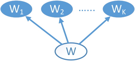
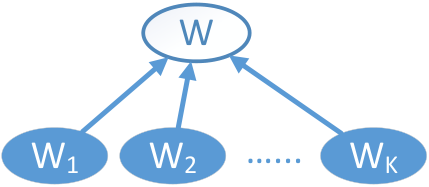
As shown in Figure 9, let $W_{f}$ be a factor window inserted “between” $W$ and its downstream windows $W_{1}$ , …, $W_{K}$ . We can do this for all “intermediate” vertices, i.e., windows with both incoming and outgoing edges, in (the augmented) WCG, thanks to the virtual “root” $S$ . Clearly, $W_{f}\leq W$ , and $W_{j}\leq W_{f}$ for $1\leq j\leq K$ . We now compare the overall computation costs with and without inserting $W_{f}$ . The cost with the factor window $W_{f}$ is $c=\sum\nolimits_{j=1}^{K}\cost(W_{j})+\cost(W_{f})+\cost(W).$ On the other hand, the cost without $W_{f}$ is $c^{\prime}=\sum\nolimits_{j=1}^{K}\cost^{\prime}(W_{j})+\cost(W).$ We define the benefit of $W_{f}$ as $\delta_{f}=c^{\prime}-c$ .

Since $\cost(W_{j})=n_{j}\cdot M(W_{j},W_{f})$ , $\cost(W_{f})=n_{f}\cdot M(W_{f},W)$ , and $\cost^{\prime}(W_{j})=n_{j}\cdot M(W_{j},W)$ , it follows that

${\color[rgb]{0,0,0}\delta_{f}=\sum\nolimits_{j=1}^{K}n_{j}\Big(M(W_{j},W)-M(W_{j},W_{f})\Big)-n_{f}M(W_{f},W).}$

By Theorem 3, $M(W_{j},W_{f})=1+(r_{j}-r_{f})/s_{f}$ , $M(W_{j},W)=1+(r_{j}-r_{W})/s_{W}$ , and $M(W_{f},W)=1+(r_{f}-r_{W})/s_{W}$ . Substituting into the above equation, we obtain

{\color[rgb]{0,0,0}\delta_{f}=\sum\nolimits_{j=1}^{K}n_{j}\Big(\frac{r_{j}-r_{W}}{s_{W}}-\frac{r_{j}-r_{f}}{s_{f}}\Big)-n_{f}\Big(1+\frac{r_{f}-r_{W}}{s_{W}}\Big).}

We now define the following quantities to simplify notation: (1) $\rho_{j}=r_{j}/r_{f}$ and $k_{j}=r_{j}/s_{j}$ , for $1\leq j\leq K$ ; (2) $k_{f}=r_{f}/s_{f}$ ; and (3) $k_{W}=r_{W}/s_{W}$ . With this notation, we have

${\color[rgb]{0,0,0}\delta_{f}=n_{f}\Big(\sum\nolimits_{j=1}^{K}\frac{n_{j}}{n_{f}}\Big(k_{f}-\frac{r_{j}}{s_{f}}+\frac{r_{j}}{s_{W}}-k_{W}\Big)-(1+\frac{r_{f}}{s_{W}}-k_{W})\Big).}$

(2)

Inserting $W_{f}$ improves if and only if $\delta_{f}\geq 0$ , i.e.,

{\color[rgb]{0,0,0}\sum\nolimits_{j=1}^{K}\frac{n_{j}}{n_{f}}\Big(k_{f}-\frac{r_{j}}{s_{f}}+\frac{r_{j}}{s_{W}}-k_{W}\Big)\geq 1+\frac{r_{f}}{s_{W}}-k_{W}.}

(3)

IV-B Candidate Generation and Selection

We can use Equation 3 to determine whether a factor window is beneficial. The next problem is to find candidate factor windows that are beneficial, from which we can select the best one. Algorithm 2 illustrates this candidate generation and selection procedure in detail.

Input:

W

, a window;

\{W_{1},...,W_{K}\}

W

’s downstream windows (ref. Figure 9).

Output: The best factor window

W_{f}

w.r.t.

W

and

\{W_{1},...,W_{K}\}

// Construct the set

\mathcal{W}_{f}

of candidate factor windows.

{\color[rgb]{0,0,0}\mathcal{W}_{f}\leftarrow\emptyset}

; 2

{\color[rgb]{0,0,0}s_{d}\leftarrow\gcd\{s_{1},...,s_{K}\}}

; 3

{\color[rgb]{0,0,0}\mathcal{S}_{f}\leftarrow\{s_{f}:s_{d}\text{ mod }s_{f}=0\text{ and }s_{f}\text{ mod }s_{W}=0\}}

; 4

{\color[rgb]{0,0,0}r_{\text{min}}\leftarrow\min\{r_{1},...,r_{K}\}}

; 5

foreach ${\color[rgb]{0,0,0}s_{f}\in\mathcal{S}_{f}}$ do 6

{\color[rgb]{0,0,0}\mathcal{R}_{f}\leftarrow\{r_{f}:r_{f}\text{ mod }s_{f}=0\text{ and }r_{f}\leq r_{\text{min}}\}}

; 7

foreach ${\color[rgb]{0,0,0}r_{f}\in\mathcal{R}_{f}}$ do 8

Construct a candidate factor window

W_{f}\langle r_{f},s_{f}\rangle

; 9

if ${\color[rgb]{0,0,0}W_{f}\leq W\text{ and }W_{j}\leq W_{f}\text{ for }1\leq j\leq K}$ then 10

{\color[rgb]{0,0,0}\mathcal{W}_{f}\leftarrow\mathcal{W}_{f}\cup\{W_{f}\}}

; 11

// Find the best factor window from

\mathcal{W}_{f}

{\color[rgb]{0,0,0}\delta_{f}^{\max}\leftarrow 0}

{\color[rgb]{0,0,0}W_{f}^{\max}\leftarrow\texttt{null}}

; 12

foreach ${\color[rgb]{0,0,0}W_{f}\in\mathcal{W}_{f}}$ do 13

Compute the benefit

\delta_{f}

W_{f}

using Equation 2; 14

if ${\color[rgb]{0,0,0}\delta_{f}\geq 0\text{ and }\delta_{f}>\delta_{f}^{\max}}$ then 15

{\color[rgb]{0,0,0}\delta_{f}^{\max}\leftarrow\delta_{f}}

{\color[rgb]{0,0,0}W_{f}^{\max}\leftarrow W_{f}}

; 16

return ${\color[rgb]{0,0,0}W_{f}^{\max}}$ ; 17

Algorithm 2 Find the best factor window under “covered by” semantics.

IV-B1 Candidate Generation

It looks for eligible slides $s_{f}$ and eligible ranges $r_{f}$ as follows (lines 2 to 2 of Algorithm 2):

•

Eligible slides: Let $s_{d}=\gcd\{s_{1},...,s_{K}\}$ . The set of eligible slides is $\mathcal{S}_{f}=\{s_{f}:s_{d}\text{ mod }s_{f}=0\text{ and }s_{f}\text{ mod }s_{W}=0\}.$ That is, $s_{f}$ must be a factor of $s_{d}$ and a multiple of $s_{W}$ .
•

Eligible ranges: Let $r_{\text{min}}=\min\{r_{1},...,r_{K}\}$ . For each $s_{f}\in\mathcal{S}_{f}$ , the set of eligible ranges is $\mathcal{R}_{f}=\{r_{f}:r_{f}\text{ mod }s_{f}=0\text{ and }r_{f}\leq r_{\text{min}}\}$ , i.e., $r_{f}\leq r_{\text{min}}$ must be a multiple of $s_{f}$ .

For each eligible pair $(s_{f},r_{f})$ , we construct a candidate factor window $W_{f}\langle r_{f},s_{f}\rangle$ and further check the window coverage constraints in Figure 9, i.e., $W_{f}\leq W$ and $W_{j}\leq W_{f}$ for $1\leq j\leq K$ (line 2), to only keep valid candidates.

IV-B2 Candidate Selection

Many candidate factor windows in $\mathcal{W}_{f}$ may be beneficial (i.e., Equation 3 holds). Only the one that leads to the maximum cost reduction (i.e., benefit) should be added. We thus compute the benefits of the candidates (by Equation 2) and select the one with the maximum benefit (lines 2 to 2 of Algorithm 2).

IV-B3 Time Complexity Analysis of Algorithm 2

Computing $s_{d}$ at line 2 takes $O(s_{\max}\log s_{\max})$ time using Euclid’s algorithm [24], where $s_{\max}=\max\{s_{1},...,s_{K}\}$ . Finding all eligible slides at line 2 takes $O(\lceil\frac{s_{d}}{s_{W}}\rceil)$ time. Computing $r_{\min}$ at line 2 takes $O(K)$ time. For each $s_{f}\in\mathcal{S}_{f}$ , finding its eligible ranges at line 2 takes $O(\lceil\frac{r_{\min}}{s_{f}}\rceil)$ time. For each $W_{f}\langle r_{f},s_{f}\rangle$ , it takes $O(K)$ time to check all related window coverage relationships at line 2. Hence, the candidate generation stage (lines 2 to 2) takes $O(s_{\max}\log s_{\max}+\lceil\frac{s_{d}}{s_{W}}\rceil+K+|\mathcal{S}_{f}|\cdot|\mathcal{R}_{f}|\cdot K)$ time. To simplify our analysis, we assume it is dominated by $O(|\mathcal{S}_{f}|\cdot|\mathcal{R}_{f}|\cdot K)$ . Now consider the candidate selection stage (lines 2 to 2). Since we check Equation 2 once for each $W_{f}$ , it takes $O(|\mathcal{S}_{f}|\cdot|\mathcal{R}_{f}|\cdot K)$ time in total. Since $|\mathcal{S}_{f}|=O(\lceil\frac{s_{d}}{s_{W}}\rceil)$ and $|\mathcal{R}_{f}|=O(\lceil\frac{r_{\min}}{s_{W}}\rceil)$ , it follows that the time complexity of Algorithm 2 is $O(\lceil\frac{s_{d}}{s_{W}}\rceil\cdot\lceil\frac{r_{\min}}{s_{W}}\rceil\cdot K)$ .

IV-C Putting Things Together

Algorithm 3 is the revised version of Algorithm 1 that returns the min-cost WCG when factor windows are allowed. It first extends the original WCG by adding the best factor windows, found by Algorithm 2, for existing windows (lines 3 to 3). It then simply invokes Algorithm 1 on the extended WCG (rather than the original one) to find the new min-cost WCG that contains factor windows (line 3).

Input:

\mathcal{W}=\{W_{i}\}_{i=1}^{n}

, a window set;

f

, aggregate function.

Output:

\mathcal{G}_{\min}

, the min-cost WCG w.r.t.

\mathcal{W}

and

f

, where factor windows are allowed.

Construct the WCG

\mathcal{G}=(\mathcal{W},\mathcal{E})

w.r.t. “covered by” or “partitioned by” determined by

f

; 1

foreach $W\in\mathcal{W}$ do 2

W_{f}\leftarrow

FindBestFactorWindow(

W

W

’s downstream windows

\{W_{1},...,W_{K}\}

) using Algorithm 2; 3

Expand

\mathcal{G}

by adding

W_{f}

and the corresponding edges (as shown in Figure 9); 4

\mathcal{G}_{\min}\leftarrow

Run lines 1-1 of Algorithm 1 over the expanded

\mathcal{G}

; 5

return the result graph $\mathcal{G}_{\min}$ ; 6

Algorithm 3 Find the min-cost WCG when factor windows are allowed.

Unlike Algorithm 1, Algorithm 3 is no longer optimal. In fact, the cost minimization problem when factor windows are allowed is an instance of the Steiner tree problem [35], which is NP-hard. Various approximate algorithms have been proposed for Steiner trees (e.g., [16, 43]), but we choose to stay with Algorithm 3 because it is simple and easy to implement. It would be interesting future work to characterize the gap between the factor windows found by Algorithm 3 and the ones that could be found by an optimal solution.³³ 3 Note that we restricted ourselves to consider only a subset of all possible factor windows. For example, for the WCG in Figure 7(a), our approach would not consider the factor window $W(15,15)$ , as $\text{gcd}\{20,30,40\}=10<15$ (ref. line 5 of Algorithm 5). An ideal, optimal solution would have also considered such candidates. In fact, it needs to generate all valid candidate factor windows, instead of finding a “locally optimal” factor window for each input window (as Algorithm 3 does), insert them into the WCG, and then solve the Steiner tree problem. Since the problem is NP-hard, the time complexity in the worst case would be exponential w.r.t. the size of the WCG. However, even though the factor windows found by Algorithm 3 may not be the optimal ones, the min-cost WCG with factor windows improves over the min-cost WCG without factor windows (returned by Algorithm 1), since Algorithm 3 only inserts a factor window if it is beneficial (lines 3 to 3).

Time Complexity Analysis of Algorithm 3

Construction of the WCG requires $O(|\mathcal{W}|^{2})$ time as it needs to check each pair of windows to test their coverage relationship. For a given window $W\in\mathcal{W}$ and its downstream windows $W_{1}$ , …, $W_{K}$ , it takes $O(\lceil\frac{s_{d}}{s_{W}}\rceil\cdot\lceil\frac{r_{\min}}{s_{W}}\rceil\cdot K)$ time to find its best factor window $W_{f}$ using Algorithm 2. Meanwhile, adding $W_{f}$ and the corresponding edges requires $O(K)$ time. Furthermore, running lines 1 to 1 of Algorithm 1 over the expanded graph takes $O((2\cdot|\mathcal{W}|)^{2})$ time. Thus, the time complexity of Algorithm 3 is $O(5|\mathcal{W}|^{2}+|\mathcal{W}|\cdot M_{\mathcal{W}})$ , where $M_{\mathcal{W}}=\max_{W\in\mathcal{W}}\{\lceil\frac{s_{d}}{s_{W}}\rceil\cdot\lceil\frac{r_{\min}}{s_{W}}\rceil\cdot K\}$ .

IV-D The Case of “Partitioned By”

We can improve the procedure FindBestFactorWindow in Algorithm 2 if we restrict the window coverage relationships to “partitioned by” semantics, which works for more types of aggregate functions. In this special case, the candidate factor windows are restricted to tumbling windows (by Theorem 4).

Input:

W_{f}

, a factor window;

W

, a target window with downstream windows

W_{1}

, …,

W_{K}

;

\lambda

, by Equation 4.

Output: Return true if adding

W_{f}

improves the overall cost, false otherwise.

if $K\geq 2$ then 1

return true; 2

// We have

K=1

hereafter.
if $k_{1}=1$ then 3

return false; 4

else 5

// We have

k_{1}>1

hereafter.
if $k_{1}\geq 3$ and $m_{1}\geq 3$ then 6

return true; 7

else 8

Compute

\frac{r_{f}}{r_{W}}

and

\frac{\lambda}{\lambda-1}=1+\frac{m_{1}}{(m_{1}-1)(k_{1}-1)}

; 9

return true if $\frac{r_{f}}{r_{W}}\geq\frac{\lambda}{\lambda-1}$ , false otherwise; 10

Algorithm 4 Determine whether a factor window would be beneficial under “partitioned by” semantics.

IV-D1 Revisit of Impact of Factor Windows

We first revisit the problem of determining whether a factor window is beneficial, under “partitioned by” semantics. Algorithm 4 summarizes the procedure that determines whether a factor window $W_{f}$ would help in the case of “partitioned by.” Here, $\lambda$ is defined as

\lambda=\sum\nolimits_{j=1}^{K}\frac{n_{j}}{m_{j}}.

(4)

The procedure in Algorithm 4 looks complicated. We offer some intuition below to help understand it:

(Case 1) If $W_{f}$ has two or more downstream windows (i.e., when $K\geq 2$ ), then it improves the overall cost (lines 4 to 4), since now at least one downstream window would benefit from reading sub-aggregates from $W_{f}$ (rather than from $W$ ). We provide more explanation using a special case (referring to Figure 9) when $K=2$ and all windows are tumbling. We can simplify Equation 2 by noticing $k_{f}=k_{W}=1$ , $r_{f}=s_{f}$ , and $r_{W}=s_{W}$ , since both $W_{f}$ and $W$ are tumbling windows: $\delta_{f}=\sum\nolimits_{j=1}^{2}n_{j}\cdot\Big(\frac{r_{j}}{r_{W}}-\frac{r_{j}}{r_{f}}\Big)-n_{f}\cdot\frac{r_{f}}{r_{W}}.$ Moreover, since all windows are tumbling, $n_{j}=m_{j}=R/r_{j}$ for $j\in\{1,2\}$ , and $n_{f}=m_{f}=R/r_{f}$ . As a result, $\delta_{f}=R\cdot\Big(\frac{1}{r_{W}}-\frac{2}{r_{f}}\Big)\geq 0,$ since $r_{f}\geq 2r_{W}$ by Theorem 4.

(Case 2) If $W_{f}$ only has one downstream window $W_{1}$ that is tumbling (i.e., the case when $K=1$ and $k_{1}=1$ ), then it cannot reduce the overall cost (lines 4 to 4) because one now needs to use all sub-aggregates from $W$ to compute $W_{f}$ itself. Without $W_{f}$ one can use the same sub-aggregates to compute $W_{1}$ directly. The case when $W_{f}$ has one unique downstream window $W_{1}$ that is not tumbling (i.e., when $K=1$ and $k_{1}>1$ ) can be understood in a similar way as “Case 1” above, since sub-aggregates from $W_{f}$ can reduce cost for intervals in $W_{1}$ that overlap (lines 4 to 4).

We formally prove the correctness of Algorithm 4 in the appendix, using Equations 2 and 4:

Theorem 8.

Algorithm 4 correctly determines whether $W_{f}$ would help when both $W_{f}$ and $W$ are tumbling windows.

IV-D2 Revisit of Candidate Generation and Selection

We now revisit the problems of candidate generation and selection under “partitioned by” semantics.

(Candidate Generation) By restricting to tumbling windows under “partitioned by” semantics, we can significantly reduce the search space for potential candidates. By Theorem 4, the range $r_{f}$ of a factor window $W_{f}$ must be a common factor of the ranges $r_{1}$ , …, $r_{K}$ of all downstream windows $W_{1}$ , …, $W_{K}$ for a given target window $W$ (ref. Figure 9). Moreover, $r_{f}$ must also be a multiple of the range $r_{W}$ of the target window $W$ . As a result, one can enumerate all candidates by starting from the greatest common divisor $r$ of $r_{1}$ , …, $r_{K}$ and look for all factors $r_{f}$ of $r$ that are also multiples of $r_{W}$ .

(Candidate Selection) To find the best factor window, we compare the benefits of two candidates $W_{f}$ and $W^{\prime}_{f}$ . There are two cases as shown in Figure 10:

•

$W_{f}$ and $W^{\prime}_{f}$ are dependent, meaning either $W_{f}\leq W^{\prime}_{f}$ or $W^{\prime}_{f}\leq W_{f}$ – see Figure 10(a);
•

$W_{f}$ and $W^{\prime}_{f}$ are independent – see Figure 10(b).

Dependent Candidates

Let $W_{f}$ and $W^{\prime}_{f}$ be two eligible factor windows such that $W^{\prime}_{f}\leq W_{f}$ . Then $W_{f}$ can be omitted as adding it cannot reduce the overall cost. This can be understood by running Algorithm 4 against $W_{f}$ , by viewing $W^{\prime}_{f}$ as $W_{f}$ ’s only (tumbling) downstream window. Algorithm 4 would return false as this is the case when $K=1$ and $k_{1}=1$ (line 4).

Independent Candidates

For the independent case, we have to compare the costs in more detail. Specifically, let $c_{f}=\sum\nolimits_{j=1}^{K}\cost(W_{j})+\cost(W_{f})+\cost(W)=\sum\nolimits_{j=1}^{K}n_{j}\cdot M(W_{j},W_{f})+n_{f}\cdot M(W_{f},W)+\cost(W),$ and $c^{\prime}_{f}=\sum\nolimits_{j=1}^{K}\cost(W_{j})+\cost(W^{\prime}_{f})+\cost(W)=\sum\nolimits_{j=1}^{K}n_{j}\cdot M(W_{j},W^{\prime}_{f})+n^{\prime}_{f}\cdot M(W^{\prime}_{f},W)+\cost(W).$

Theorem 9.

Let $W_{f}$ and $W^{\prime}_{f}$ be two independent eligible factor windows under “partitioned by” semantics. $c_{f}\leq c^{\prime}_{f}$ iff

\frac{r_{f}}{r^{\prime}_{f}}\geq\frac{\lambda-\frac{r_{f}}{r_{W}}}{\lambda-\frac{r^{\prime}_{f}}{r_{W}}}.

(5)

Here $\lambda$ has been defined in Equation 4.

Input:

W

, a window;

\{W_{1},...,W_{K}\}

W

’s downstream windows (ref. Figure 9).

Output: The best tumbling factor window

W_{f}

that led to the minimum overall cost.

Compute

\lambda

using Equation 4; 1

// Generate candidate tumbling factor windows.

r_{d}\leftarrow\gcd(\{r_{1},...,r_{K}\})

; 2

if $r_{d}=r_{W}$ then 3

return $W$ ; 4

\mathcal{F}\leftarrow\{r_{f}:r_{d}\text{ mod }r_{f}=0\text{ and }r_{f}\text{ mod }r_{W}=0\}

; 5

\mathcal{W}_{f}\leftarrow\emptyset

; 6

foreach $r_{f}\in\mathcal{F}$ do 7

Create a tumbling window

W_{f}\langle r_{f},r_{f}\rangle

; 8

b\leftarrow

Check(

W_{f}

W

\{W_{1},...,W_{K}\},\lambda

) by Algorithm 4; 9

if $b=$ true then 10

\mathcal{W}_{f}\leftarrow\mathcal{W}_{f}\cup\{W_{f}

}; 11

// Remove candidates that are not independent.
foreach $W_{f}\in\mathcal{W}_{f}$ do 12

if there exists $W^{\prime}_{f}$ s.t. $W^{\prime}_{f}\leq W_{f}$ then 13

\mathcal{W}_{f}\leftarrow\mathcal{W}_{f}-\{W_{f}\}

; 14

return the best $W_{f}\in\mathcal{W}_{f}$ by applying Theorem 9; 15

Algorithm 5 Find the best factor window under “partitioned by” semantics.

Algorithm 5 presents the details of picking the best factor window for a target window $W$ and its downstream windows $W_{1}$ , …, $W_{K}$ , under “partitioned by” semantics. It starts by enumerating all candidates for $W_{f}$ based on the constraint that $r_{f}$ must be a common factor of $\{r_{1},...,r_{K}\}$ and a multiple of $r_{W}$ (lines 5 to 5). It simply returns $W$ if no candidate can be found (line 5). It then looks for candidates of $W_{f}$ that are beneficial, using Algorithm 4 (lines 5 to 5). It further prunes dependent candidates that are dominated by others (lines 5 to 5). Finally, it finds the best $W_{f}$ by applying Theorem 9 to compare the remaining candidates.

Example 8.

Continuing with Example 7, Algorithm 5 would generate three candidate factor windows $W(10,10)$ , $W(5,5)$ , and $W(2,2)$ , since all of them are beneficial according to Algorithm 4 ( $K=2$ indeed). However, since both $W(5,5)$ and $W(2,2)$ cover $W(10,10)$ , these two candidates are removed and $W(10,10)$ is the remaining, best candidate.

Time Complexity Analysis of Algorithm 5

Computing $\lambda$ at line 5 takes $O(K)$ time. Computing $r_{d}$ at line 5 takes $O(r_{\max}\log r_{\max})$ time using Euclid’s algorithm [24], where $r_{\max}=\max\{r_{1},...,r_{K}\}$ . Computing $\mathcal{F}$ at line 5 takes $O(\lceil\frac{r_{d}}{r_{W}}\rceil)$ time. Generating candidate tumbling factor windows (lines 5 to 5) takes $O(|\mathcal{F}|)$ time, as each run of Algorithm 4 takes constant time. Pruning dependent candidates (lines 5 to 5) takes $O(|\mathcal{F}|^{2})$ time due to pairwise comparison. Finally, finding the best candidate by applying Theorem 9 takes $O(|\mathcal{F}|)$ time. Therefore, the time complexity of Algorithm 5 is $O(K+r_{\max}\log r_{\max}+\lceil\frac{r_{d}}{r_{W}}\rceil+|\mathcal{F}|^{2}+2\cdot|\mathcal{F}|).$ To simplify our analysis, we assume it is dominated by $O(|\mathcal{F}|^{2})$ . Since $O(|\mathcal{F}|)=O(\lceil\frac{r_{d}}{r_{W}}\rceil)$ , it follows that the time complexity of Algorithm 5 is $O(\lceil\frac{r_{d}}{r_{W}}\rceil^{2})$ . This is in contrast to the $O(\lceil\frac{s_{d}}{s_{W}}\rceil\cdot\lceil\frac{r_{\min}}{s_{W}}\rceil\cdot K)$ time complexity of Algorithm 2, which finds the best factor window following “covered by” semantics. In a real-world setting, we would expect $\lceil\frac{r_{\min}}{s_{W}}\rceil>\lceil\frac{r_{d}}{r_{W}}\rceil\approx\lceil\frac{s_{d}}{s_{W}}\rceil$ , in which case Algorithm 5 improves over Algorithm 2 significantly. On the other hand, Algorithm 5 may lose some optimization opportunities due to its reduced search space for candidate factor windows. We only use Algorithm 5 when “covered by” semantics cannot be used to optimize the input aggregate function.

(a) RandomGen, “partitioned by”

(b) RandomGen, “covered by”

(d) SequentialGen, “covered by”

Fig. 11: Throughput on window sets when processing 10 million input events from Synthetic-10M with

|\mathcal{W}|=5

V Evaluation

We report experimental evaluation results in this section. We observe that (1) the optimized query plan, even without factor windows, can significantly outperform the original query plan in terms of throughput [34] (up to 2.5 $\times$ ); (2) with factor windows, the throughput of the optimized query plan can be much higher (up to 16.8 $\times$ ). Moreover, our optimized plans can yield similar, and sometimes much higher, throughput compared to Scotty [49], one state-of-the-art window slicing technique. Meanwhile, our approach has negligible overhead and can scale up smoothly when increasing window-set size.

V-A Experiment Settings

V-A1 Setup

We implemented our cost-based query optimizer in C#. Given an input window-set aggregate query with its original query plan, it can produce the best query plans, with and without factor windows. All query plans are represented as Trill expressions. For each query plan, we measure its throughput, which is defined as the number of events processed per unit time [34]. We perform all experiments on a workstation equipped with 2.2 GHz Intel CPUs and 128 GB main memory. All results are based on single-core executions.

V-A2 Data Sets

We used both synthetic and real data. For synthetic data, we generated data streams with 1 million and 10 million events, denoted as Synthetic-1M and Synthetic-10M respectively, where the events arrive at a constant pace. For real data, we used the same dataset as used in [17], which was derived from the DEBS 2012 Grand Challenge [33] dataset that consists of monitoring data from manufacturing equipment. Specifically, we pair the given timestamps with the values of the column mf01, i.e., the “electrical power main-phase 1” sensor reading. This dataset contains roughly 32 million events and is denoted as Real-32M. We used “MIN” as the aggregate function, which can be supported by both “covered by” and “partitioned by” semantics.

Input:

S

, the “seed” slides;

R

, the “seed” ranges;

k_{s}

k_{r}

: the multipliers;

N

, the size of the window set; tumbling: whether each window is tumbling or not.

Output:

\mathcal{W}

, the window set generated.

\mathcal{W}\leftarrow\emptyset

; 1

for $1\leq i\leq N$ do 2

if tumbling then 3

r_{0}\leftarrow

Random(

R

); 4

r\leftarrow

Random(

\{2r_{0},...,k_{r}\cdot r_{0}\}

); 5

\mathcal{W}\leftarrow\mathcal{W}\cup\{W\langle r,r\rangle\}

; 6

else 7

s_{0}\leftarrow

Random(

S

); 8

s\leftarrow

Random(

\{2s_{0},...,k_{s}\cdot s_{0}\}

); 9

\mathcal{W}\leftarrow\mathcal{W}\cup\{W\langle 2s,s\rangle\}

; 10

return the window set $\mathcal{W}$ ; 11

Algorithm 6 The RandomGen window-set generator.

V-A3 Generation of Window Sets

We generated window sets using the following approaches.

•

(RandomGen) We generate each window $W\langle r,s\rangle$ randomly. Specifically, to generate a tumbling window where $s=r$ , we first pick a “seed” range $r_{0}$ uniformly randomly from a given list and then choose $r$ uniformly randomly from $\{2r_{0},...,k_{r}\cdot r_{0}\}$ . We purposely avoid choosing $r=r_{0}$ to test the effectiveness of our cost-based optimizer when exploring factor windows, as $W\langle r_{0},r_{0}\rangle$ is a valid factor window in this case that should be considered by the optimizer. To generate a hopping window, we operate in a similar manner by first picking a “seed” slide $s_{0}$ uniformly randomly from a given list and then choosing $s$ uniformly randomly among $\{2s_{0},...,k_{s}\cdot s_{0}\}$ ; we finally set $r=2s$ and return $W\langle r,s\rangle$ . Algorithm 6 summarizes this procedure.
•

(SequentialGen) In practice, the windows contained by a window set may be more correlated than those generated by RandomGen. Here, we focus on a common case that we observed in the real world, where the windows follow a “sequential” pattern in terms of either the range or the slide size. We presented such an example in Figure 1. This motivates us to implement the SequentialGen window-set generator that aims for capturing this sequential pattern. Specifically, unlike in RandomGen where $r$ is randomly selected from $\{2r_{0},...,k_{r}\cdot r_{0}\}$ when generating tumbling windows , we simply pick $r$ sequentially following the order $2r_{0}$ , …, $k_{r}\cdot r_{0}$ . Similarly, we pick $s$ sequentially following the order $2s_{0}$ , …, $k_{s}\cdot s_{0}$ when generating hopping windows.

V-B Results on Synthetic Data

For the parameters in RandomGen and SequentialGen, we set the window-set size $N\in\{5,10\}$ , the “seed” slides $S=\{5,10,20\}$ (only for generating hopping windows, where ranges are fixed as twice the slides), the “seed” ranges $R=\{2,5,10\}$ (only for generating tumbling windows), and $k_{s}=k_{r}=50$ . For each window-set size $N$ , we generated 10 window sets for both tumbling and hopping windows. We also set $\eta=1$ in our cost model.

V-B1 Throughput

Figure 11 reports the throughput results observed on Synthetic-10M for window sets of size 5 generated by both RandomGen and SequentialGen. The results on Synthetic-10M with window sets of size 10, as well as the results on Synthetic-1M are included in the appendix.

Observations on window sets by RandomGen

(1) For the window sets containing tumbling windows, the “partitioned by” semantics were leveraged when constructing the window coverage graph (WCG) and exploring factor windows. As illustrated in Figure 11(a), compared to the original plan, the rewritten plan without factor windows can boost throughput by up to 1.9 $\times$ , whereas the plan with factor windows can boost the throughput by up to 2.5 $\times$ . (2) For the window sets containing hopping windows, the general “covered by” semantics were used to create WCG’s and factor windows. Figure 11(b) presents the results. We observe similar patterns as we observed on tumbling windows, where factor windows yield significantly larger throughput (by up to 4.3 $\times$ ). (3) In a couple of cases, the optimized plans are slightly worse than the original plans. This is possible, since our cost model does not use throughput as the cost metric. However, such cases are rare based on our evaluation, and in the appendix we show that our cost metric is highly correlated with throughput.

Observations on window sets by SequentialGen

The observations are similar to those on window sets generated by RandomGen. Again, using factor windows significantly boosts the throughput (by up to 4.8 $\times$ and 2.8 $\times$ for “partitioned by” and “covered by” semantics, respectively). We further notice that the rewritten query plans without factor windows are more effective than they were in the case of RandomGen. This is not surprising, though, as the improved correlation between windows generated by SequentialGen leads to more overlaps and thus more sharing opportunities.

Setup	w/o FW (Mean)	w/o FW (Max)	w/ FW (Mean)	w/ FW (Max)
R-5-tumbling	1.21 $\times$	1.92 $\times$	1.85 $\times$	2.54 $\times$
R-10-tumbling	1.34 $\times$	1.77 $\times$	1.88 $\times$	3.38 $\times$
R-5-hopping	1.18 $\times$	1.82 $\times$	3.26 $\times$	4.29 $\times$
R-10-hopping	1.34 $\times$	1.71 $\times$	3.20 $\times$	6.15 $\times$
S-5-tumbling	1.63 $\times$	1.67 $\times$	4.28 $\times$	4.81 $\times$
S-10-tumbling	1.98 $\times$	2.05 $\times$	7.91 $\times$	9.38 $\times$
S-5-hopping	1.34 $\times$	1.48 $\times$	2.17 $\times$	2.81 $\times$
S-10-hopping	1.58 $\times$	1.73 $\times$	2.92 $\times$	3.79 $\times$

TABLE I: Summary of throughput boosts on Synthetic-10M, where ‘R’ stands for window sets generated by RandomGen, ‘S’ stands for window sets generated by SequentialGen, and ‘5’ and ‘10’ are the sizes of the window sets generated.

Summary

In Table I, we summarize the mean and max throughput boosts of the rewritten query plans (without and with factor windows) over the original query plans, observed when processing Synthetic-10M under different experimental setups for window-set generation. With factor windows, we can achieve up to 9.4 $\times$ throughput boost on Synthetic-10M.

Setup	w/o FW (Mean)	w/o FW (Max)	w/ FW (Mean)	w/ FW (Max)
R-5-tumbling	1.19 $\times$	1.78 $\times$	1.43 $\times$	1.91 $\times$
R-10-tumbling	1.30 $\times$	1.71 $\times$	1.53 $\times$	2.86 $\times$
R-5-hopping	1.09 $\times$	1.39 $\times$	1.54 $\times$	2.63 $\times$
R-10-hopping	1.18 $\times$	1.39 $\times$	1.46 $\times$	3.53 $\times$
S-5-tumbling	1.63 $\times$	1.67 $\times$	4.12 $\times$	4.85 $\times$
S-10-tumbling	1.90 $\times$	1.97 $\times$	7.53 $\times$	9.14 $\times$
S-5-hopping	1.12 $\times$	1.30 $\times$	1.22 $\times$	1.77 $\times$
S-10-hopping	1.22 $\times$	1.51 $\times$	1.45 $\times$	2.31 $\times$

TABLE II: Summary of throughput boosts on Real-32M, with the same notation as in Table I.

V-C Results on Real Data

We further tested the throughput of window sets over the real dataset Real-32M. Table II summarizes the results on throughput boosts of the rewritten query plans, without and with factor windows, over the original plans, and the details are included in the appendix. Overall, using factor windows can achieve throughput boost up to 9.1 $\times$ over Real-32M.

V-D Scalability Tests

To understand the scalability of our cost-based optimization approach, we increased the window-set size $|\mathcal{W}|$ to 15 and 20. Table III summarizes the throughput results on Synthetic-10M; the details are in the appendix. Overall, the query plans generated by our approach scale up smoothly when increasing the window-set size, with throughput boost up to 16.8 $\times$ .

Setup	w/o FW (Mean)	w/o FW (Max)	w/ FW (Mean)	w/ FW (Max)
R-15-tumbling	1.55 $\times$	1.96 $\times$	2.97 $\times$	4.34 $\times$
R-20-tumbling	1.49 $\times$	2.29 $\times$	2.10 $\times$	4.83 $\times$
R-15-hopping	1.55 $\times$	1.95 $\times$	4.67 $\times$	6.59 $\times$
R-20-hopping	1.68 $\times$	2.20 $\times$	4.23 $\times$	7.65 $\times$
S-15-tumbling	2.43 $\times$	2.49 $\times$	11.29 $\times$	13.83 $\times$
S-20-tumbling	2.42 $\times$	2.53 $\times$	14.28 $\times$	16.82 $\times$
S-15-hopping	1.85 $\times$	2.09 $\times$	3.51 $\times$	4.68 $\times$
S-20-hopping	1.91 $\times$	2.15 $\times$	4.02 $\times$	5.32 $\times$

TABLE III: Summary of results on scalability test with

\mathcal{W}\in\{15,20\}

, in terms of throughput boosts on Synthetic-10M. The notation here is the same as in Tables I and II.

V-E Query Optimization Overhead

Fig. 12: Factor-window based optimization overhead (average time and standard deviation) with increasing window-set size from 5 to 20. ‘R’ and ‘S’ are shorthands for “RandomGen” and “SequentialGen”.

Figure 12 presents the average time spent on query optimization and its standard deviation (shown with error bars), when enabling factor windows and varying window-set size from 5 to 20. For each setting, the average and standard deviation were measured based on the 10 window sets generated by either RandomGen or SequentialGen. We observe that the optimization overhead is very small overall ( $<$ 100 milliseconds for the settings that we tested). Moreover, the optimization overhead of “covered by” semantics is higher than that of “partitioned by” semantics. This makes sense considering the larger search space with “covered by” semantics.

(a) RandomGen, “partitioned by”

(b) RandomGen, “covered by”

(d) SequentialGen, “covered by”

Fig. 13: Comparison with Scotty [49] in terms of throughput on window sets with

|\mathcal{W}|=10

V-F Comparison with Window Slicing

We compare our cost-based optimization approach with Scotty [49], one state-of-the-art window slicing technology. Since Scotty does not support Trill, we translate our optimized query plans into Apache Flink queries expressed by its DataStream API [2], following a similar query rewriting procedure described in Section III-C. We compare the throughput of Flink, Scotty, and our optimized plans with factor windows, using the same data generator developed by Scotty for benchmarking its own performance [49, 5]. In our experiments we set the window-set size $|\mathcal{W}|\in\{5,10\}$ . We did not further increase $|\mathcal{W}|$ since Scotty cannot process some window sets with $|\mathcal{W}|=10$ (see Figure 13(a)). Figure 13 shows the results with $|\mathcal{W}|=10$ . The results with $|\mathcal{W}|=5$ are in the appendix.

We have two observations. First, both Scotty and our factor-window based optimization significantly outperform the default Flink query execution plan, where each window aggregate is evaluated independently. Second, our approach can yield similar, and sometimes much higher, throughput compared to Scotty. This holds for both window sets generated by RandomGen (Figures 13(a) and 13(b)) and SequentialGen (Figures 13(c) and 13(d)), where we observe up to 5.7 $\times$ throughput boost (excluding cases where the throughput of Scotty is unavailable).

VI Related Work

The related work on stream query processing and optimization is overwhelming (see [32] for a survey). We focus our discussion on optimization techniques dedicated to window aggregates [19, 38]. In addition to the window slicing techniques discussed in the introduction (e.g. [36, 37, 30, 31, 20, 45, 48, 49]), there has been a flurry of recent work that accelerates window aggregation via better utilization of modern hardware, such as Grizzly [28] and LightSaber [46]. This line of work is orthogonal to ours. However, it may be worthwhile to consider combining it with our cost-based optimization framework, which we leave for future work.

Cost-based query optimization is the standard practice in batch processing systems [44], but is not popular in stream processing systems. There is little work on cost modeling in the streaming world [51]. One reason might be the difficulty of defining a single cost criterion, as streaming systems may need to honor various performance metrics simultaneously, such as latency, throughput, and resource utilization [22]. Although the application of static cost-based query optimization is limited [12], dynamic query optimization (a.k.a., adaptive query processing) at runtime has been extensively studied in the context of streaming (e.g., [11, 15, 25, 26, 39, 40, 41, 42, 50]). Our current cost model is static and it is interesting future work to investigate how to dynamically adjust cost estimates at runtime by keeping track of the input event rates.

In recent years, a number of distributed streaming systems have been built as open-source or proprietary software (e.g., Storm [47], Spark Streaming [10], Flink [18], MillWheel [7], Dataflow [8], Quill [21], etc.). While most of these systems provide users with imperative programming interfaces, the adoption of declarative, SQL-like query interfaces [9], similar to the one that ASA exposes, has been increasingly popular. For example, both Spark Streaming and Flink now support SQL queries on top of data streams. Moving to the declarative interface raises the level of abstraction and enables compile-time query optimization. The optimization techniques proposed in this paper can be implemented in either imperative or declarative systems. We demonstrated the latter for the ASA SQL query compiler (Section III-C), but our algorithms are not tied to the ASA SQL language and can be applied in other streaming systems that support declarative query languages.

VII Conclusion

We proposed a cost-based optimization framework to optimize the evaluation of aggregate functions over multiple correlated windows. It leverages the window coverage graph (WCG) that we introduced to capture the inherent overlapping relationships between windows. We introduced factor windows into the WCG to help reduce the overall computation overhead. Evaluation results show that the optimized query plans can significantly outperform the original plans in terms of throughput, especially when factor windows are enabled, without the need for runtime support from stream processing engines.

References

[1] Amazon kinesis. https://aws.amazon.com/kinesis/.
[2] Apache flink datastream api. https://nightlies.apache.org/flink/flink-docs-release-1.14/docs/dev/datastream/overview/.
[3] Azure iot central. https://azure.microsoft.com/en-us/services/iot-central/.
[4] Azure stream analytics. https://azure.microsoft.com/en-us/services/stream-analytics/.
[5] Github repository of scotty. https://github.com/TU-Berlin-DIMA/scotty-window-processor.
[6] Google cloud dataflow. https://cloud.google.com/dataflow/.
[7] T. Akidau, A. Balikov, K. Bekiroglu, S. Chernyak, J. Haberman, R. Lax, S. McVeety, D. Mills, P. Nordstrom, and S. Whittle. Millwheel: Fault-tolerant stream processing at internet scale. PVLDB, 6(11), 2013.
[8] T. Akidau, R. Bradshaw, C. Chambers, S. Chernyak, R. Fernández-Moctezuma, R. Lax, S. McVeety, D. Mills, F. Perry, E. Schmidt, and S. Whittle. The dataflow model: A practical approach to balancing correctness, latency, and cost in massive-scale, unbounded, out-of-order data processing. PVLDB, 8(12):1792–1803, 2015.
[9] A. Arasu, S. Babu, and J. Widom. The CQL continuous query language: semantic foundations and query execution. VLDB J., 15(2), 2006.
[10] M. Armbrust, T. Das, J. Torres, B. Yavuz, S. Zhu, R. Xin, A. Ghodsi, I. Stoica, and M. Zaharia. Structured streaming: A declarative API for real-time applications in apache spark. In SIGMOD, 2018.
[11] R. Avnur and J. M. Hellerstein. Eddies: Continuously adaptive query processing. In SIGMOD, pages 261–272, 2000.
[12] A. Ayad and J. F. Naughton. Static optimization of conjunctive queries with sliding windows over infinite streams. In SIGMOD, 2004.
[13] R. S. Barga, J. Goldstein, M. H. Ali, and M. Hong. Consistent streaming through time: A vision for event stream processing. In CIDR, pages 363–374, 2007.
[14] L. Benson, P. M. Grulich, S. Zeuch, V. Markl, and T. Rabl. Disco: Efficient distributed window aggregation. In EDBT, 2020.
[15] P. A. Bernstein, T. Porter, R. Potharaju, A. Z. Tomsic, S. Venkataraman, and W. Wu. Serverless event-stream processing over virtual actors. In CIDR, 2019.
[16] J. Byrka, F. Grandoni, T. Rothvoß, and L. Sanità. An improved lp-based approximation for steiner tree. In STOC, pages 583–592, 2010.
[17] W. Cai, P. A. Bernstein, W. Wu, and B. Chandramouli. Optimization of threshold functions over streams. Proc. VLDB Endow., 14(6), 2021.
[18] P. Carbone, A. Katsifodimos, S. Ewen, V. Markl, S. Haridi, and K. Tzoumas. Apache flink™: Stream and batch processing in a single engine. IEEE Data Eng. Bull., 38(4):28–38, 2015.
[19] P. Carbone, A. Katsifodimos, and S. Haridi. Stream window aggregation semantics and optimization. In S. Sakr and A. Y. Zomaya, editors, Encyclopedia of Big Data Technologies. Springer, 2019.
[20] P. Carbone, J. Traub, A. Katsifodimos, S. Haridi, and V. Markl. Cutty: Aggregate sharing for user-defined windows. In CIKM, pages 1201–1210, 2016.
[21] B. Chandramouli, R. C. Fernandez, J. Goldstein, A. Eldawy, and A. Quamar. Quill: Efficient, transferable, and rich analytics at scale. PVLDB, 9(14):1623–1634, 2016.
[22] B. Chandramouli, J. Goldstein, R. S. Barga, M. Riedewald, and I. Santos. Accurate latency estimation in a distributed event processing system. In ICDE, pages 255–266, 2011.
[23] B. Chandramouli, J. Goldstein, M. Barnett, R. DeLine, J. C. Platt, J. F. Terwilliger, and J. Wernsing. Trill: A high-performance incremental query processor for diverse analytics. PVLDB, 8(4):401–412, 2014.
[24] T. H. Cormen, C. E. Leiserson, R. L. Rivest, and C. Stein. Introduction to algorithms. MIT press, 2009.
[25] A. Deshpande and J. M. Hellerstein. Lifting the burden of history from adaptive query processing. In VLDB, pages 948–959, 2004.
[26] A. Floratou, A. Agrawal, B. Graham, S. Rao, and K. Ramasamy. Dhalion: Self-regulating stream processing in heron. PVLDB, 10(12):1825–1836, 2017.
[27] J. Gray, S. Chaudhuri, A. Bosworth, A. Layman, D. Reichart, M. Venkatrao, F. Pellow, and H. Pirahesh. Data cube: A relational aggregation operator generalizing group-by, cross-tab, and sub totals. Data Min. Knowl. Discov., 1(1):29–53, 1997.
[28] P. M. Grulich, S. Breß, S. Zeuch, J. Traub, J. von Bleichert, Z. Chen, T. Rabl, and V. Markl. Grizzly: Efficient stream processing through adaptive query compilation. In SIGMOD, pages 2487–2503.
[29] Z. Gu, M. A. Soliman, and F. M. Waas. Testing the accuracy of query optimizers. In E. Lo and F. Waas, editors, DBTest, page 11, 2012.
[30] S. Guirguis, M. A. Sharaf, P. K. Chrysanthis, and A. Labrinidis. Optimized processing of multiple aggregate continuous queries. In CIKM, pages 1515–1524, 2011.
[31] S. Guirguis, M. A. Sharaf, P. K. Chrysanthis, and A. Labrinidis. Three-level processing of multiple aggregate continuous queries. In ICDE, pages 929–940, 2012.
[32] M. Hirzel, R. Soulé, S. Schneider, B. Gedik, and R. Grimm. A catalog of stream processing optimizations. ACM Comput. Surv., 46(4):46:1–46:34, 2013.
[33] Z. Jerzak, T. Heinze, M. Fehr, D. Gröber, R. Hartung, and N. Stojanovic. The DEBS 2012 grand challenge. In DEBS, pages 393–398, 2012.
[34] J. Karimov, T. Rabl, A. Katsifodimos, R. Samarev, H. Heiskanen, and V. Markl. Benchmarking distributed stream data processing systems. In ICDE, pages 1507–1518, 2018.
[35] R. M. Karp. Reducibility among combinatorial problems. In Complexity of Computer Computations, pages 85–103, 1972.
[36] S. Krishnamurthy, C. Wu, and M. J. Franklin. On-the-fly sharing for streamed aggregation. In SIGMOD, pages 623–634, 2006.
[37] J. Li, D. Maier, K. Tufte, V. Papadimos, and P. A. Tucker. No pane, no gain: efficient evaluation of sliding-window aggregates over data streams. SIGMOD Record, 34(1):39–44, 2005.
[38] J. Li, D. Maier, K. Tufte, V. Papadimos, and P. A. Tucker. Semantics and evaluation techniques for window aggregates in data streams. In SIGMOD, pages 311–322, 2005.
[39] L. Mai, K. Zeng, R. Potharaju, L. Xu, S. Suh, S. Venkataraman, P. Costa, T. Kim, S. Muthukrishnan, V. Kuppa, S. Dhulipalla, and S. Rao. Chi: A scalable and programmable control plane for distributed stream processing systems. PVLDB, 11(10):1303–1316, 2018.
[40] R. V. Nehme, E. A. Rundensteiner, and E. Bertino. Self-tuning query mesh for adaptive multi-route query processing. In EDBT, pages 803–814, 2009.
[41] R. V. Nehme, K. Works, C. Lei, E. A. Rundensteiner, and E. Bertino. Multi-route query processing and optimization. J. Comput. Syst. Sci., 79(3):312–329, 2013.
[42] V. Raman, A. Deshpande, and J. M. Hellerstein. Using state modules for adaptive query processing. In ICDE, pages 353–364, 2003.
[43] G. Robins and A. Zelikovsky. Improved steiner tree approximation in graphs. In SODA, pages 770–779, 2000.
[44] P. G. Selinger, M. M. Astrahan, D. D. Chamberlin, R. A. Lorie, and T. G. Price. Access path selection in a relational database management system. In SIGMOD, pages 23–34, 1979.
[45] K. Tangwongsan, M. Hirzel, S. Schneider, and K. Wu. General incremental sliding-window aggregation. PVLDB, 8(7):702–713, 2015.
[46] G. Theodorakis, A. Koliousis, P. R. Pietzuch, and H. Pirk. Lightsaber: Efficient window aggregation on multi-core processors. In SIGMOD, pages 2505–2521.
[47] A. Toshniwal, S. Taneja, A. Shukla, K. Ramasamy, J. M. Patel, S. Kulkarni, J. Jackson, K. Gade, M. Fu, J. Donham, N. Bhagat, S. Mittal, and D. V. Ryaboy. Storm@twitter. In SIGMOD, pages 147–156, 2014.
[48] J. Traub, P. M. Grulich, A. R. Cuellar, S. Breß, A. Katsifodimos, T. Rabl, and V. Markl. Efficient window aggregation with general stream slicing. In EDBT, pages 97–108, 2019.
[49] J. Traub, P. M. Grulich, A. R. Cuellar, S. Breß, A. Katsifodimos, T. Rabl, and V. Markl. Scotty: General and efficient open-source window aggregation for stream processing systems. ACM Trans. Database Syst., 46(1):1:1–1:46, 2021.
[50] S. Venkataraman, A. Panda, K. Ousterhout, M. Armbrust, A. Ghodsi, M. J. Franklin, B. Recht, and I. Stoica. Drizzle: Fast and adaptable stream processing at scale. In SOSP, pages 374–389, 2017.
[51] S. Viglas and J. F. Naughton. Rate-based query optimization for streaming information sources. In SIGMOD, pages 37–48, 2002.
[52] W. Wu. A note on operator-level query execution cost modeling. CoRR, abs/2003.04410, 2020.
[53] W. Wu, X. Wu, H. Hacigümüs, and J. F. Naughton. Uncertainty aware query execution time prediction. Proc. VLDB Endow., 7(14), 2014.
[54] M. Zaharia, T. Das, H. Li, T. Hunter, S. Shenker, and I. Stoica. Discretized streams: fault-tolerant streaming computation at scale. In SOSP, pages 423–438, 2013.

(a) RandomGen, “partitioned by”

(b) RandomGen, “covered by”

(d) SequentialGen, “covered by”

Fig. 14: Throughput on window sets when processing 10 million input events from Synthetic-10M with

|\mathcal{W}|=10

(a) RandomGen, “partitioned by”

(b) RandomGen, “covered by”

(d) SequentialGen, “covered by”

Fig. 15: Throughput on window sets when processing 1 million input events from Synthetic-1M with

|\mathcal{W}|=5

(a) RandomGen, “partitioned by”

(b) RandomGen, “covered by”

(d) SequentialGen, “covered by”

Fig. 16: Throughput on window sets when processing 1 million input events from Synthetic-1M with

|\mathcal{W}|=10

(a) RandomGen, “partitioned by”

(b) RandomGen, “covered by”

(d) SequentialGen, “covered by”

Fig. 17: Throughput when processing 32 million input events from Real-32M with

|\mathcal{W}|=5

(a) RandomGen, “partitioned by”

(b) RandomGen, “covered by”

(d) SequentialGen, “covered by”

Fig. 18: Throughput when processing 32 million input events from Real-32M with

|\mathcal{W}|=10

(a) RandomGen, “partitioned by” (

r=0.98

)

(b) RandomGen, “covered by” (

r=0.95

)

r=0.94

)

(d) SequentialGen, “covered by” (

r=0.94

)

Fig. 19: Correlation between predicted ‘speedup’ by the cost model and observed ‘speedup’ on throughput over Synthetic-10M.

(a) RandomGen, “partitioned by”

(b) RandomGen, “covered by”

(d) SequentialGen, “covered by”

Fig. 20: Throughput on window sets when processing 10 million input events from Synthetic-10M with

|\mathcal{W}|=15

(a) RandomGen, “partitioned by”

(b) RandomGen, “covered by”

(d) SequentialGen, “covered by”

Fig. 21: Throughput on window sets when processing 10 million input events from Synthetic-10M with

|\mathcal{W}|=20

(a) RandomGen, “partitioned by”

(b) RandomGen, “covered by”

(d) SequentialGen, “covered by”

Fig. 22: Comparison with Scotty [49] in terms of throughput on window sets with

|\mathcal{W}|=5

Appendix A Proofs

A-A Proof of Theorem 1

Proof.

Consider an arbitrary interval $I=[a,b)\in W_{1}$ . By the interval representation of $W_{1}$ , we have $a=m_{1}\cdot s_{1}$ and $b=m_{1}\cdot s_{1}+r_{1}$ for some integer $m_{1}\geq 0$ .

The “if” part $\Rightarrow$ : Since $s_{1}$ is a multiple of $s_{2}$ , we have $s_{1}=k\cdot s_{2}$ for some integer $k\geq 1$ . As a result,

m_{1}\cdot s_{1}=m_{1}\cdot k\cdot s_{2}=(m_{1}\cdot k)\cdot s_{2}.

Similarly, since $\delta_{r}=r_{1}-r_{2}$ is a multiple of $s_{2}$ , $r_{1}-r_{2}=k^{\prime}\cdot s_{2}$ for some integer $k^{\prime}\geq 1$ . As a result,

	$\displaystyle m_{1}\cdot s_{1}+r_{1}$	$\displaystyle=$	$\displaystyle(m_{1}\cdot k)\cdot s_{2}+k^{\prime}\cdot s_{2}+r_{2}$
		$\displaystyle=$	$\displaystyle(m_{1}\cdot k+k^{\prime})\cdot s_{2}+r_{2}.$

Set $m_{2}=m_{1}\cdot k$ and $m^{\prime}_{2}=m_{1}\cdot k+k^{\prime}$ . Now consider two intervals $I_{a}=[a,x)=[m_{2}\cdot s_{2},m_{2}\cdot s_{2}+r_{2})$ and $I_{b}=[y,b)=[m^{\prime}_{2}\cdot s_{2},m^{\prime}_{2}\cdot s_{2}+r_{2})$ that belong to $W_{2}$ . Clearly, we have

m_{2}\cdot s_{2}=m_{1}\cdot s_{1}=a

and

m^{\prime}_{2}\cdot s_{2}+r_{2}=m_{1}\cdot s_{1}+r_{1}=b.

Moreover, since $m^{\prime}_{2}>m_{2}$ , we have $x=m_{2}\cdot s_{2}+r_{2}<b$ and $y=m^{\prime}_{2}\cdot s_{2}>a$ . Therefore, $W_{1}$ is covered by $W_{2}$ , by Definition 1.

2.

The “only if” part $\Leftarrow$ : Since $W_{1}$ is covered by $W_{2}$ , by Definition 1 there exist two intervals $I_{a}=[a,x)$ and $I_{b}=[y,b)$ in $W_{2}$ such that $x<b$ and $y>a$ . As a result, there is some $m_{2}\geq 0$ such that $m_{2}\cdot s_{2}=a=m_{1}\cdot s_{1}$ . That is,

$m_{2}=m_{1}\cdot(s_{1}/s_{2}).$

Since both $m_{1}$ and $m_{2}$ are integers, $s_{1}/s_{2}$ is also an integer. As a result, $s_{1}$ must be a multiple of $s_{2}$ .

On the other hand, similarly there is some $m^{\prime}_{2}>m_{2}$ such that

$m^{\prime}_{2}\cdot s_{2}+r_{2}=b=m_{1}\cdot s_{1}+r_{1}.$

We then have

$m^{\prime}_{2}\cdot s_{2}+r_{2}=m_{2}\cdot s_{2}+r_{1},$

which yields

$m^{\prime}_{2}=m_{2}+(r_{1}-r_{2})/s_{2}.$

Since both $m^{\prime}_{2}$ and $m_{2}$ are integers, $(r_{1}-r_{2})/s_{2}$ must be an integer. Hence, $\delta_{r}=r_{1}-r_{2}$ is a multiple of $s_{2}$ .

This completes the proof of the theorem. ∎

A-B Proof of Theorem 2

Proof.

We prove the three properties one by one.

1.

Reflexivity: Clearly, by Definition 1 a window $W$ is covered by itself.
2.

Antisymmetry: Suppose that $W_{1}\leq W_{2}$ and $W_{2}\leq W_{1}$ . Consider an arbitrary interval $[a,b)$ contained by $W_{1}$ . Since $W_{1}\leq W_{2}$ , there exist two intervals $I_{x}=[a,x)$ and $I_{y}=[y,b)$ in $W_{2}$ . On the other hand, since $W_{2}\leq W_{1}$ , for $I_{x}$ there exist intervals $I_{x^{\prime}}=[a,x^{\prime})$ and $I_{x^{\prime\prime}}=[x^{\prime\prime},x)$ in $W_{1}$ . Since no two intervals in a window start from the same time point but end at different time points, we conclude that

$x^{\prime}=b.$

Since $x^{\prime}\leq x\leq b$ by Definition 1, we have

$x=x^{\prime}=x^{\prime\prime}=b.$

Using similar arguments we can show that $y=y^{\prime}=y^{\prime\prime}=a$ . As a result, we have proved that $W_{1}=W_{2}$ .
3.

Transitivity: Suppose that $W_{1}\leq W_{2}$ and $W_{2}\leq W_{3}$ . Again, consider an arbitrary interval $[a,b)$ in $W_{1}$ . Since $W_{1}\leq W_{2}$ , there exist two intervals $I_{x}=[a,x)$ and $I_{y}=[y,b)$ in $W_{2}$ . Moreover, since $W_{2}\leq W_{3}$ , there exist two intervals $I_{x^{\prime}}=[a,x^{\prime})$ and $I_{x^{\prime\prime}}=[x^{\prime\prime},x)$ in $W_{3}$ , and there also exist two intervals $I_{y^{\prime}}=[y,y^{\prime})$ and $I_{y^{\prime\prime}}=[y^{\prime\prime},b)$ in $W_{3}$ . Now consider $I_{x^{\prime}}$ and $I_{y^{\prime\prime}}$ . By Definition 1, we have $x^{\prime}\leq x\leq b$ and $y^{\prime\prime}\geq y\geq a$ . Since $[a,b)$ is an arbitrary interval in $W_{1}$ , it follows that $W_{1}\leq W_{3}$ .

This completes the proof of the theorem. ∎

A-C Proof of Theorem 3

Proof.

If we take a union of the intervals in $\mathcal{I}_{a,b}$ , it is easy to see $I=\cup_{J\in\mathcal{I}_{a,b}}J$ . By Definition 1, we can further enumerate the intervals in $\mathcal{I}_{a,b}$ as $J_{1}=[x_{1},y_{1})$ , …, $J_{n}=[x_{n},y_{n})$ such that $x_{1}=a$ , $y_{n}=b$ , and $x_{1}<\cdots<x_{n}$ , where $n=|\mathcal{I}_{a,b}|$ . Therefore,

I=J_{1}\cup(J_{2}-J_{1})\cup\cdots\cup(J_{n}-J_{n-1}).

Since the intervals $J_{1}$ , $J_{2}-J_{1}$ , …, $J_{n}-J_{n-1}$ are mutually exclusive, it follows that

|I|=|J_{1}|+|J_{2}-J_{1}|+\cdots+|J_{n}-J_{n-1}|.

We have $|I|=r_{1}$ , $|J_{1}|=r_{2}$ , and $|J_{k}-J_{k-1}|=s_{2}$ for $2\leq k\leq n$ . As a result, $r_{1}=r_{2}+(n-1)\cdot s_{2},$ which yields

M(W_{1},W_{2})=n=1+(r_{1}-r_{2})/s_{2}.

This completes the proof of the theorem. ∎

A-D Proof of Theorem 4

Proof.

We prove each direction separately.

(a)

The “if” part $\Rightarrow$ : Suppose that conditions (1) to (3) hold. By (2) and (3), we know that $r_{1}-r_{2}$ must be a multiple of $s_{2}$ either. Combining with (1), $W_{1}$ is covered by $W_{2}$ according to Theorem 1. Now consider an arbitrary interval $I$ in $W_{1}$ . Let the covering set of $I$ in $W_{2}$ be $\mathcal{I}$ . We next show that $\mathcal{I}$ is disjoint. By (2) and (3) we know that $r_{1}$ is a multiple of $r_{2}$ . As a result, $r_{1}=k\cdot r_{2}$ where $k$ is an integer. To show that $\mathcal{I}$ is disjoint we only need to show that $|\mathcal{I}|=k$ (recall Figure 4(a)). We have

$\displaystyle\|\mathcal{I}\|$	$\displaystyle=$	$\displaystyle 1+(r_{1}-r_{2})/s_{2},\qquad\text{[by Theorem~\ref{theorem:covering-multiplier}]}$
	$\displaystyle=$	$\displaystyle 1+(k\cdot r_{2}-r_{2})/s_{2},\qquad\text{[by Condition (2)]}$
	$\displaystyle=$	$\displaystyle 1+(k-1),\qquad\text{[by Condition (3)]}$
	$\displaystyle=$	$\displaystyle k.$

(b)

The “only if” part $\Leftarrow$ : Suppose that $W_{1}$ is partitioned by $W_{2}$ . By Theorem 1, condition (1) holds. Again, consider an arbitrary interval $I$ in $W_{1}$ and let its covering set in $W_{2}$ be $\mathcal{I}$ . We know that $\mathcal{I}$ is disjoint, which implies condition (3), i.e., $r_{2}=s_{2}$ , as well as that $r_{1}$ must be a multiple of $r_{2}$ . Therefore, $r_{1}$ must also be a multiple of $s_{2}$ and condition (2) holds.

This completes the proof of the theorem. ∎

A-E Proof of Theorem 6

Proof.

We only prove MIN is distributive over overlapping partitions, as the proof for MAX is very similar. We set both $f$ and $g$ in the definition of distributive aggregate function as MIN. It is easy to see that, if two sets $S_{1}$ and $S_{2}$ satisfying $S_{1}\subseteq S_{2}$ , then $\verb|MIN|(S_{2})\leq\verb|MIN|(S_{1})$ .⁴⁴ 4 We treat each element in $T$ differently, even if some of them may have the same data value. Moreover, for any set $S$ , $\verb|MIN|(S)\in S$ and thus $\{\verb|MIN|(S)\}\subseteq S$ . Therefore,

S=\{\verb|MIN|(T_{1}),...,\verb|MIN|(T_{n})\}\subseteq T_{1}\cup\cdots\cup T_{n},

since $\verb|MIN|(T_{1})\subseteq T_{1}$ , …, $\verb|MIN|(T_{n})\subseteq T_{n}$ . As a result,

\verb|MIN|(T)\leq\verb|MIN|(S)=\verb|MIN|(\{\verb|MIN|(T_{1}),...,\verb|MIN|(T_{n})\}).

We now prove that $\verb|MIN|(S)\leq\verb|MIN|(T)$ . To see this, let

$\displaystyle S_{1}$	$\displaystyle=$	$\displaystyle T_{1},$
$\displaystyle S_{2}$	$\displaystyle=$	$\displaystyle T_{2}-T_{1},$
$\displaystyle S_{3}$	$\displaystyle=$	$\displaystyle T_{3}-(S_{1}\cup S_{2}),$
	$\displaystyle...$
$\displaystyle S_{n}$	$\displaystyle=$	$\displaystyle T_{n}-(S_{1}\cup\cdots\cup S_{n-1}).$

We have $T=S_{1}\cup\cdots\cup S_{n}$ , and $S_{i}\cap S_{j}=\emptyset$ for all $1\leq i,j\leq n$ . Therefore, $\verb|MIN|(T)=\verb|MIN|(S_{1}\cup\cdots\cup S_{n})$ . Moreover, there exists some $j$ such that $\verb|MIN|(S_{j})=\verb|MIN|(T)$ . Since $S_{j}\subseteq T_{j}$ , $\verb|MIN|(S_{j})\geq\verb|MIN|(T_{j})$ . As a result,

$\displaystyle\verb\|MIN\|(T)$	$\displaystyle=$	$\displaystyle\verb\|MIN\|(\{\verb\|MIN\|(S_{1}),...,\verb\|MIN\|(S_{n})\})$
	$\displaystyle\geq$	$\displaystyle\verb\|MIN\|(\{\verb\|MIN\|(T_{1}),...,\verb\|MIN\|(T_{n})\})$
	$\displaystyle=$	$\displaystyle\verb\|MIN\|(S).$

Since we have proved both $\verb|MIN|(S)\leq\verb|MIN|(T)$ and $\verb|MIN|(T)\leq\verb|MIN|(S)$ , it must hold that $\verb|MIN|(S)=\verb|MIN|(T)$ . ∎

A-F Proof of Theorem 8

Since both $W_{f}$ and $W$ in Figure 9 are now tumbling windows, $k_{f}=k_{W}=1$ . Equation 3 then yields

\sum\nolimits_{j=1}^{K}\frac{n_{j}}{n_{f}}\Big(\frac{r_{j}}{s_{f}}-\frac{r_{j}}{s_{W}}\Big)+\frac{r_{f}}{s_{W}}\leq 0.

Since $r_{f}=s_{f}$ and $r_{W}=s_{W}$ , it follows that

\sum\nolimits_{j=1}^{K}\frac{n_{j}}{n_{f}}\Big(\rho_{j}-\frac{r_{j}}{r_{W}}\Big)+\frac{r_{f}}{r_{W}}\leq 0.

Since $r_{f}=\frac{r_{j}}{\rho_{j}}$ by definition, we have $r_{j}=\rho_{j}r_{f}$ and thus

\sum\nolimits_{j=1}^{K}\frac{n_{j}\rho_{j}}{n_{f}}\Big(1-\frac{r_{f}}{r_{W}}\Big)+\frac{r_{f}}{r_{W}}\leq 0.

(6)

Moreover, by definition of $n_{f}$ (Equation 1) we have

n_{f}=(m_{f}-1)k_{f}+1=m_{f}=\frac{R}{r_{f}}=\frac{R\rho_{j}}{r_{j}}=m_{j}\rho_{j}.

Substituting into Equation 6, it follows that

\Big(1-\frac{r_{f}}{r_{W}}\Big)\cdot\lambda+\frac{r_{f}}{r_{W}}\leq 0,

(7)

where $\lambda$ has been defined in Equation 4. As a result, we have

\frac{r_{f}}{r_{W}}\geq\frac{\lambda}{\lambda-1}.

(8)

Since $n_{j}=(m_{j}-1)k_{j}+1\geq m_{j}$ , by Equation 4 we have $\lambda\geq K$ . We distinguish two cases: $K\geq 2$ and $K=1$ .

The Case of $K\geq 2$

When $K\geq 2$ we have

\frac{\lambda}{\lambda-1}\leq\frac{K}{K-1}\leq 2.

Since $\frac{r_{f}}{r_{W}}\geq 2$ , Equation 8 holds, which implies $c\leq c^{\prime}$ . Note that the equality $c=c^{\prime}$ only holds when $r_{f}=2r_{W}$ and $\lambda=K=2$ , which implies $n_{j}=m_{j}$ for $j=1,2$ . In this case, both downstream windows of $W$ (and thus $W_{f}$ ) are tumbling, and $W_{f}$ exactly doubles the range of $W$ , which is a very special case.

The Case of $K=1$

When $K=1$ , $\lambda=\frac{n_{1}}{m_{1}}$ . We distinguish two situations:

•

If $k_{1}=1$ , which means that the (unique) downstream window is tumbling, then $n_{1}=m_{1}$ and thus $\lambda=1$ . Equation 7 then implies that $1\leq 0$ , which is impossible. As a result, $c\leq c^{\prime}$ does not hold.

•

If $k_{1}>1$ , then $\lambda>1$ and thus the RHS of Equation 8 is well-defined. Note that we must have $m_{1}>1$ , since if $m_{1}=1$ then $n_{1}=(m_{1}-1)k_{1}+1=1$ and thus $\lambda=1$ , a contradiction. Substituting $\lambda=\frac{n_{1}}{m_{1}}$ , we obtain

$\displaystyle\frac{\lambda}{\lambda-1}$	$\displaystyle=$	$\displaystyle 1+\frac{m_{1}}{n_{1}-m_{1}}$
	$\displaystyle=$	$\displaystyle 1+\frac{m_{1}}{(m_{1}-1)(k_{1}-1)}$
	$\displaystyle=$	$\displaystyle 1+\frac{1}{k_{1}-1}+\frac{1}{(m_{1}-1)(k_{1}-1)}.$

As a result, when $k_{1}\geq 3$ and $m_{1}\geq 3$ ,

\frac{\lambda}{\lambda-1}\leq 1+\frac{1}{2}+\frac{1}{4}<2,

and thus Equation 8 holds without equality as $r_{f}\geq 2r_{W}$ , which implies $c<c^{\prime}$ . For the other two special cases where one of $k_{1}$ and $m_{1}$ is 2 and the other is 3, we have to compare the LHS and RHS to determine whether Equation 8 holds.

A-G Proof of Theorem 9

Let $d=c_{f}-c^{\prime}_{f}$ . It then follows that

$\displaystyle d$	$\displaystyle=$	$\displaystyle\sum\nolimits_{j=1}^{K}n_{j}\Big(M(W_{j},W_{f})-M(W_{j},W^{\prime}_{f})\Big)+\Delta$	(9)
	$\displaystyle=$	$\displaystyle\sum\nolimits_{j=1}^{K}n_{j}\Big(\frac{r_{j}-r_{f}}{s_{f}}-\frac{r_{j}-r^{\prime}_{f}}{s^{\prime}_{f}}\Big)+\Delta$
	$\displaystyle=$	$\displaystyle\sum\nolimits_{j=1}^{K}n_{j}\Big(\frac{r_{j}}{s_{f}}-k_{f}-\frac{r_{j}}{s^{\prime}_{f}}+k^{\prime}_{f}\Big)+\Delta,$

where

$\displaystyle\Delta$	$\displaystyle=$	$\displaystyle n_{f}\cdot M(W_{f},W)-n^{\prime}_{f}\cdot M(W^{\prime}_{f},W)$
	$\displaystyle=$	$\displaystyle n_{f}\Big(1+\frac{r_{f}-r_{W}}{s_{W}}\Big)-n^{\prime}_{f}\Big(1+\frac{r^{\prime}_{f}-r_{W}}{s_{W}}\Big)$
	$\displaystyle=$	$\displaystyle n_{f}\Big(1+\frac{r_{f}}{s_{W}}-k_{W}\Big)-n^{\prime}_{f}\Big(1+\frac{r^{\prime}_{f}}{s_{W}}-k_{W}\Big).$

Clearly, $W_{f}$ is more beneficial if $d<0$ .

Proof.

Since $W_{f}$ , $W^{\prime}_{f}$ , and $W$ are all tumbling windows, $k_{f}=k^{\prime}_{f}=k_{W}=1$ . Substituting into Equation 9 and using the facts $r_{f}=s_{f}$ , $r^{\prime}_{f}=s^{\prime}_{f}$ , and $r_{W}=s_{W}$ yields

	$\displaystyle c_{f}-c^{\prime}_{f}$	$\displaystyle=$	$\displaystyle\sum\nolimits_{j=1}^{K}n_{j}\Big(\frac{r_{j}}{r_{f}}-\frac{r_{j}}{r^{\prime}_{f}}\Big)+n_{f}\cdot\frac{r_{f}}{r_{W}}-n^{\prime}_{f}\cdot\frac{r^{\prime}_{f}}{r_{W}}$
		$\displaystyle=$	$\displaystyle n_{f}\Big(\sum\nolimits_{j=1}^{K}\frac{n_{j}}{n_{f}}\Big(\frac{r_{j}}{r_{f}}-\frac{r_{j}}{r^{\prime}_{f}}\Big)+\frac{r_{f}}{r_{W}}-\frac{n^{\prime}_{f}}{n_{f}}\cdot\frac{r^{\prime}_{f}}{r_{W}}\Big).$

Again we consider when $c_{f}\leq c^{\prime}_{f}$ holds. Or equivalently,

\sum\nolimits_{j=1}^{K}\frac{n_{j}}{n_{f}}\Big(\frac{r_{j}}{r_{f}}-\frac{r_{j}}{r^{\prime}_{f}}\Big)+\frac{r_{f}}{r_{W}}-\frac{n^{\prime}_{f}}{n_{f}}\cdot\frac{r^{\prime}_{f}}{r_{W}}\leq 0.

Similarly, define

\rho_{j}=\frac{r_{j}}{r_{f}},\quad\rho^{\prime}_{j}=\frac{r_{j}}{r^{\prime}_{f}},\quad\forall 1\leq j\leq K.

Since $W_{f}$ is tumbling,

n_{f}=m_{f}=\frac{R}{r_{f}}=\frac{m_{j}r_{j}}{r_{f}}=m_{j}\rho_{j}.

It therefore follows that

\sum\nolimits_{j=1}^{K}\frac{n_{j}}{m_{j}\rho_{j}}(\rho_{j}-\rho^{\prime}_{j})+\frac{r_{f}}{r_{W}}-\frac{n^{\prime}_{f}}{n_{f}}\cdot\frac{r^{\prime}_{f}}{r_{W}}\leq 0.

Noting that

\frac{\rho^{\prime}_{j}}{\rho_{j}}=\frac{r_{j}/r^{\prime}_{f}}{r_{j}/r_{f}}=\frac{r_{f}}{r^{\prime}_{f}}

and making some rearrangement of the terms yields

\Big(1-\frac{r_{f}}{r^{\prime}_{f}}\Big)\sum\nolimits_{j=1}^{K}\frac{n_{j}}{m_{j}}+\frac{r^{\prime}_{f}}{r_{W}}\Big(\frac{r_{f}}{r^{\prime}_{f}}-\frac{n^{\prime}_{f}}{n_{f}}\Big)\leq 0.

As before, define $\lambda=\sum\nolimits_{j=1}^{K}\frac{n_{j}}{m_{j}}$ . It then follows that

\frac{r_{f}}{r^{\prime}_{f}}\geq\frac{\lambda-\frac{r^{\prime}_{f}}{r_{W}}\cdot\frac{n^{\prime}_{f}}{n_{f}}}{\lambda-\frac{r^{\prime}_{f}}{r_{W}}}.

Moreover, since both $W_{f}$ and $W^{\prime}_{f}$ are tumbling windows, we have $n_{f}=m_{f}$ and $n^{\prime}_{f}=m^{\prime}_{f}$ . Therefore,

\frac{r^{\prime}_{f}}{r_{W}}\cdot\frac{n^{\prime}_{f}}{n_{f}}=\frac{r^{\prime}_{f}}{r_{W}}\cdot\frac{m^{\prime}_{f}}{m_{f}}=\frac{R}{r_{W}m_{f}}=\frac{r_{f}}{r_{W}},

which yields

\frac{r_{f}}{r^{\prime}_{f}}\geq\frac{\lambda-\frac{r_{f}}{r_{W}}}{\lambda-\frac{r^{\prime}_{f}}{r_{W}}}.

This completes the proof of the theorem. ∎

Appendix B Query Rewriting for Trill

Formally, given $\mathcal{G}_{\min}$ that captures the optimal window coverage relationships, the query rewriting algorithm works as follows. Suppose that the original plan is

\text{Input Stream}\Rightarrow\verb|MultiCast|\Rightarrow\mathcal{W}=\{W_{1},...,W_{n}\}\Rightarrow\verb|Union|.

We first replace $\mathcal{W}$ by the min-cost WCG $\mathcal{G}_{\min}$ :

\text{Input Stream}\Rightarrow\verb|MultiCast|\Rightarrow\mathcal{G}_{\min}\Rightarrow\verb|Union|.

We then perform the following steps:

•

For each window $w$ (in $\mathcal{G}_{\min}$ ) without an incoming edge, create a link from MultiCast to $w$ . Remove the MultiCast operator if there is only one such $w$ .
•

For each (intermediate) window $v$ with outgoing edges, insert a MultiCast operator $M_{v}$ . Create a link from $v$ to $M_{v}$ and a link from $M_{v}$ to Union. For each $(v,u)$ of $v$ ’s outgoing edges, create a link from $M_{v}$ to $u$ .
•

For each window $w$ without outgoing edges, create a link from $w$ to Union.

Appendix C More Evaluation Results

C-A Results on Synthetic Data

Figure 14 presents the details of the throughput results on window sets over the Synthetic-10M dataset when setting the window-set size $|\mathcal{W}|=10$ . Figures 15 and 16 further present the details of the throughput results on window sets over the Synthetic-1M dataset, and we summarize the results in Table IV. Overall, we observe similar patterns on Synthetic-10M and Synthetic-1M.

Setup	w/o FW (Mean)	w/o FW (Max)	w/ FW (Mean)	w/ FW (Max)
R-5-tumbling	1.21 $\times$	2.01 $\times$	1.85 $\times$	2.41 $\times$
R-10-tumbling	1.36 $\times$	1.72 $\times$	1.94 $\times$	3.13 $\times$
R-5-hopping	1.19 $\times$	1.76 $\times$	2.90 $\times$	3.78 $\times$
R-10-hopping	1.31 $\times$	1.54 $\times$	2.94 $\times$	5.14 $\times$
S-5-tumbling	1.63 $\times$	1.79 $\times$	3.82 $\times$	4.43 $\times$
S-10-tumbling	1.91 $\times$	2.07 $\times$	6.27 $\times$	7.27 $\times$
S-5-hopping	1.33 $\times$	1.51 $\times$	2.10 $\times$	2.73 $\times$
S-10-hopping	1.54 $\times$	1.69 $\times$	2.75 $\times$	3.65 $\times$

TABLE IV: Summary of throughput boosts on Synthetic-1M, where ‘R’ stands for window sets generated by RandomGen, ‘S’ stands for window sets generated by SequentialGen, and ‘5’ and ‘10’ are the sizes of the window sets generated.

C-B Results on Real Data

Figures 17 and 18 present the details of the throughput results on the real dataset Real-32M when setting the window-set size $|\mathcal{W}|$ to $|\mathcal{W}|=5$ and $|\mathcal{W}|=10$ , respectively. Again, we observe that the throughput when using factor windows is often significantly higher than that when factor windows were not considered. We also observe that, even just using the rewritten plans without including factor windows can often significantly outperform the original plans.

C-C Effectiveness of Cost Model

To test the effectiveness of our cost model developed in Section III, we measure the correlation [29, 53, 52] between the observed throughput boost and the estimated cost reduction using the cost model on Synthetic-10M, given that the constant input event rate of Synthetic-10M matches the underlying assumption of our cost model. Specifically, let the throughput of the rewritten query plans, without and with factor windows, be $T_{\text{w/o}}$ and $T_{\text{w/}}$ , respectively, and we define the throughput speedup as $\gamma_{T}=\frac{T_{\text{w/}}}{T_{\text{w/o}}}$ . Moreover, let the estimated costs of the rewritten query plans, without and with factor windows, be $C_{\text{w/o}}$ and $C_{\text{w/}}$ , respectively, and we define the estimated speedup as $\gamma_{C}=\frac{C_{\text{w/o}}}{C_{\text{w/}}}$ . We are interested in the correlation between $\gamma_{T}$ and $\gamma_{C}$ . Figure 19 presents the results of this correlation test. In each chart, the $x$ -axis represents $\gamma_{C}$ whereas the $y$ -axis represents $\gamma_{T}$ , and we have merged data points from both $|\mathcal{W}|=5$ and $|\mathcal{W}|=10$ . Overall, we observe very strong correlation between $\gamma_{T}$ and $\gamma_{C}$ , regardless of the experiment setup (e.g., RandomGen vs. SequentialGen, “partitioned by” vs. “covered by”). We further calculated the Pearson correlation coefficient $r$ for each chart, and we observe that $r\geq 0.94$ in all cases that we tested.

C-D Scalability Tests

Figures 20 and 21 present the details of our scalability test on Synthetic-10M when setting the window-set size $|\mathcal{W}|\in\{15,20\}$ . We observe similar patterns to that when setting $|\mathcal{W}|\in\{5,10\}$ , which suggests that the optimized query plans produced by our cost-based approach can scale up smoothly with increasing window-set size.

C-E Comparison with Window Slicing

Figure 22 presents the results that compare the throughput of Apache Flink, Scotty, and our factor-window based optimization when setting the window-set size $|\mathcal{W}|=5$ . We observe that our approach and Scotty result in similar throughput, and both approaches significantly outperform the default query plan used by Apach Flink that evaluates each window aggregate independently.

$\displaystyle\verb\|MIN\|(T)$	$\displaystyle=$	$\displaystyle\verb\|MIN\|(\{\verb\|MIN\|(S_{1}),...,\verb\|MIN\|(S_{n})\})$
	$\displaystyle\geq$	$\displaystyle\verb\|MIN\|(\{\verb\|MIN\|(T_{1}),...,\verb\|MIN\|(T_{n})\})$
	$\displaystyle=$	$\displaystyle\verb\|MIN\|(S).$