跳到论文正文
W Papers独立论文阅读器 arXiv:2008.12323 论文正文 计算阅读时间 · 0%
引用这篇论文根据当前论文元数据生成,正式投稿前建议核对。


License: arXiv.org perpetual non-exclusive license
arXiv:2008.12323v1 [cs.IT] 27 Aug 2020

, ,

Gridless Multidimensional Angle of Arrival Estimation for Arbitrary 3D Antenna ArraysM. Sánchez-Fernández is with Universidad Carlos III de Madrid, Spain. V. Jamali is with University of Erlangen-Nuremberg, Germany. A. Tulino, and J. Llorca are with New York University, NY. A. Tulino is with University of Naples Federico II, Italy.

Matilde Sánchez-Fernández    Vahid Jamali    Jaime Llorca    Antonia Tulino
Abstract

A full multi–dimensional characterization of the AoA (AoA) has immediate applications to the efficient operation of modern wireless communication systems. In this work, we develop a compressed sensing based method to extract multi-dimensional AoA information exploiting the sparse nature of the signal received by a sensor array. The proposed solution, based on the atomic ℓ0\ell_{0} norm, enables accurate gridless resolution of the AoA in systems with arbitrary 3D antenna arrays. Our approach allows characterizing the maximum number of distinct sources (or scatters) that can be identified for a given number of antennas and array geometry. Both noiseless and noisy measurement scenarios are addressed, deriving and evaluating the resolvability of the AoA propagation parameters through a multi–level Toeplitz matrix rank\rank–minimization problem. To facilitate the implementation of the proposed solution, we also present a least squares approach regularized by a convex relaxation of the rank\rank-minimization problem and characterize its conditions for resolvability.

Index Terms: 
Multi–dimensional AoA, atomic norm, 33D antenna array, multi–level Vandermonde decomposition.

I Introduction

Optimizing the performance of wireless communication systems critically relies on extracting relevant information from the wireless propagation channel. Array processing techniques have been extensively used to reveal, extract, and exploit key propagation parameters such as AoA and AoD (AoD) in order to tailor and optimize the transmission to individual users in systems with multiple antennas [1].

In particular, AoA (and analogously AoD) estimation refers to the process of retrieving multi–dimensional direction of propagation parameters (e.g., azimuth, elevation) associated with possibly multiple electromagnetic sources (e.g., transmitters, scatters), from the observation of a receiving vector 𝐲{\mathbf{y}}, whose elements represent the signal outputs at each of the receiving antennas that form a sensor array. The received signal associated with a given source k∈{1,…,K}k\in\{1,\ldots,K\} impinging on an NN-antenna array from direction (θk,ϕk)(\theta_{k},\phi_{k}) can be represented by a so-called steering vector 𝐫N​(θk,ϕk)∈ℂN{\mathbf{r}}_{N}\left(\theta_{k},\phi_{k}\right)\in{\mathbb{C}}^{N}, characterized by the relative phase shifts at each of the antennas. The observable 𝐲{\mathbf{y}} is hence a noisy linear combination of such steering vectors, one for each source. The goal is to identify each steering vector and extract their associated multi–dimensional AoA parameters, represented by multi–dimensional frequencies, from the observation of 𝐲{\mathbf{y}}.

Existing methods for angular characterization of signal propagation include initial beamforming–based approaches [2] (highly limited in their resolution), covariance-based subspace methods such as Capon’s beamformer, MUSIC (MUSIC), ESPRIT (ESPRIT), and their extensions [3, 4], and (determistic) ML (ML) methods based on NLS (NLS) optimization problems [3]. However, all aforementioned methods suffer from well–known limitations. Subspace and NLS based methods require a priori knowledge of the number of sources, which may be difficult to obtain in practice. Capon’s beamformer, MUSIC, and ESPRIT need accurate estimates of the observable covariance matrix, which in turn requires a slow time-varying environment, a large number of observations (to build the sample covariance matrix), and a low level of source correlation (to avoid rank deficiency in the sample covariance matrix). In addition, NLS algorithms require very accurate initialization since their objective function has a complicated multimodal shape with a sharp global minimum.

On the other hand, an important observation is that AoA estimation can be seen as a sparse data representation/separation problem, where compressed sensing methods [5] can be used to significantly enhance accuracy and robustness. In particular, compressed sensing does not require any statistical knowledge of the parameters to be estimated or associated observations. Hence, it avoids the need to estimate the observable covariance matrix or even having prior knowledge of the number of sources to identify, while still providing strong performance guarantees. Such obliviousness to the number of sources and the statistics of the received signals makes compressed sensing techniques notably suitable to overcome the limitations of previous approaches in terms of robustness to mismatches with respect to prior knowledge.

The estimation of AoA information via compressed sensing techniques can be classified into three main categories: on–grid, off–grid, and gridless estimation. Despite AoA being an intrinsically continuous variable, initial approaches for AoA estimation using sparse methods were based on sampling the angular space, forcing the angles to be estimated to lay on a discrete grid [6, 7]. The problem with this approach is clear – even with very fine gridding, there is always a mismatch between grid and real values. Off–grid solutions try to overcome this mismatch by means of adaptive grids [8] or by estimating and compensating the grid offset [9]. Finally, gridless approaches do not rely on any discretization of the angular space – they directly operate in the continuous domain, completely avoiding the grid mismatch problem, at the expense of increased computational complexity [10, 11].

A number of recent works have studied the use of gridless compressed sensing techniques for AoA estimation. However, most of them have only been applied to the estimation of 11D AoA parameters in [10, 11, 12, 13], and only more recently, to multidimensional scenarios, with applications to uniform antenna arrays in [14, 15], and allowing non-uniform deployments in [16, 17].

It is important to note that non–uniform 33D deployments are becoming increasingly relevant in upcoming 55G/66G communication paradigms such as EMB (EMB), MMT (MMT), or URLL (URLL) communications, where high rates, low latency, massive connectivity, and extremely accurate localization require a level of multi–dimensional space awareness that can only be achieved with arrays of matching dimensionality. Importantly, 33D arrays rarely deploy antennas uniformly, since they typically follow cubic [18] or cylindrical [19] geometries without antennas deployed inside the volume.

I-A Contributions

In this work, we focus on the design of robust an efficient techniques for i) full–dimensional AoA estimation in systems with ii) arbitrary antenna deployments. We leverage compressed sensing techniques that exploit the sparse nature of signal measurements impinging on arbitrary multi–dimensional antenna arrays. The approach undertaken is based on sparse approximation of the signal impinging on a 33D antenna array and the use of the Vandermonde decomposition to enable gridless extraction of multi–dimensional propagation parameters that are intrinsically continuous variables (see [11, 12, 14]). It is worth highlighting that while the application scenario considered in this paper focuses on 33D array deployments where the goal is the gridless extraction of dd-dimensional parameters with d≤3d\leq 3, the results derived in Section III hold for multi–dimensional parameters of arbitrary dimensionality dd.

Our main contributions can be summarized as follows:

In the noiseless setting:

  • •

    Given a receiving NN-antenna array following an arbitrary dd-dimensional configuration, we characterize the resolvable region, i.e., the maximum number of resolvable sources (e.g., scatters) KK and their associated dd-dimensional propagation parameters, referred to as frequencies. We show that the size of the resolvable region grows linearly with the number of antennas, not only in the uniform setting, but also with non–uniform arrays. Specifically, the maximum number of resolvable scatters is given by ⌊S𝖼−(d−1)2⌋\left\lfloor\frac{S_{{\mathsf{c}}}-(d-1)}{2}\right\rfloor, where S𝖼S_{{\mathsf{c}}} is the sum of the number of antennas in each dimension of the largest uniform array embedded in the original structure. We further strongly conjecture, as validated by our numerical results, that the maximum number of resolvable scatters is in fact given by ⌈N𝖼2−1⌉\left\lceil\frac{N_{{\mathsf{c}}}}{2}-1\right\rceil, where N𝖼N_{{\mathsf{c}}} is the total number of antennas in the largest uniform array embedded in the original structure. Importantly, the resolvable region characterized in this work i) is larger than the region already available in literature [14] and ii) has more general applicability, since it can be used with measurements coming from non-uniform sampled observations.

  • •

    For the case of non-uniform deployments with large number of antennas (e.g., massive MIMO (MIMO) systems), we show that the large-scale nature of the array deployment allows guaranteeing resolvability with probability 1−ϵ1-\epsilon of up to KK scatters with N=O⁡(K​log⁡(K/ϵ))N=O(K\log(K/\epsilon)) independently of the specific array geometry.

  • •

    The aforementioned characterization follows a novel constructive approach that allows not only identifies the resolvable scatters, but also extracts the associated dd-dimensional propagation parameters. Such approach consists of three steps: First, the NN-dimensional observable vector 𝐲{\mathbf{y}} is represented as a sampled version of an enlarged N¯\bar{N}-dimensional vector 𝐬{\mathbf{s}} composed of a linear combination of uniform steering vectors associated with the smallest uniform array covering each of the original antennas, referred to as virtual uniform array. In the second step, we find the minimum number of steering vectors that compose 𝐬{\mathbf{s}} by reformulating the minimization of the ℓ0\ell_{0}- AN (AN) of 𝐬{\mathbf{s}} as the search for a min\min-rank\rank dd-dimensional MLT (MLT) matrix. A distinctive feature of our approach is to restrict this search to a specific PSD (PSD) matrix set, termed canonical (see Definition 4), that is shown to preserve optimality, while significantly reducing the required dimension of the virtual uniform array N¯\bar{N}. Finally, in the third step, we show that the multilevel Vandermonde decomposition of the resulting min\min-rank\rank dd-MLT canonical matrix allows the extraction of the dd-dimensional propagation parameters.

  • •

    The proposed rank\rank minimization based approach is NP-hard in general, and its traditional convex counterpart based on ℓ1\ell_{1}-AN and trace minimization is known to exhibit significant limitations [11]. Most prominently, the resulting ℓ1\ell_{1}-AN and trace minimizer is not guaranteed to be sparse. To circumvent this problem, we resort to a weighted ℓ2\ell_{2}+ℓ1\ell_{1}-AN minimization method. We numerically show the advantage of the proposed approach in overcoming the drawbacks of the ℓ1\ell_{1}-AN convex approximation.

  • •

    Noting that the complexity of the proposed rank\rank and trace minimization based methods is driven by the size of the virtual uniform array, our approach allows finding the dd-dimensional propagation parameters of any number of scatters in the resolvable region KK using a virtual uniform array with at least KK antennas along its largest dimension, leading to a complexity that scales (exponentially for ℓ0\ell_{0}-AN and polynomially for ℓ1\ell_{1}-AN) with KK. This result significantly outperforms the existing best known result in [14] that requires a virtual uniform array with at least KK antennas along its smallest dimension, resulting in a complexity that scales (exponentially or polynomially) with KdK^{d}. The reduced requirement on the dimension of the virtual uniform array is a consequence of a novel generalization of the Carathéodory-Fejér theorem, which allows enlarging the set of PSD dd-MLT matrices that admit a unique Vandermonde decomposition (see Lemma 1).

In the noisy setting:

  • •

    For the case of noisy measurements, we resort to the weighted ℓ2\ell_{2}+ℓ1\ell_{1}-AN optimization approach and provide a closed-form expression for the weight as a function of the signal-to-noise ratio 𝖲𝖭𝖱\mathsf{SNR}, which is shown to well approximate the numerically computed optimal value. We evaluate the performance of our approach for moderate and high 𝖲𝖭𝖱\mathsf{SNR}, showing an estimation error very close to the associated CRLB (CRLB).

General array design guidelines:

  • •

    Our results suggest that if the goal is identifying up to KK scatters (and extract their associated dd–dimensional propagation parameters), we should design an antenna array whose smallest uniform embedded structure has at least 2​K2K antennas, where most of them are lying along a dominate dimension, while maintaining at least 22 antennas in the other dimensions. While 2​(K+1)2(K+1) antennas, independent of geometry, allows resolving KK scatters, a design with a dominant dimension will help resolving the KK scatters with complexity O⁡(K)O(K) instead of O⁡(Kd)O(K^{d}).

I-B Related work

We now describe results and limitations of the compressed sensing based studies that are more closely related to our work. We emphasize that the limitations of such previous results arise from the fact of requiring more stringent conditions for frequency recovery and/or lacking applicability to general array structures.

In terms of the resolvable region, the best known result, provided in [14], bounds the number of resolvable scatters KK by the minimum number of antennas in each of the dd dimensions of the antenna array. In contrast, we significantly enlarge the resolvable region by bounding the number of resolvable scatters by the maximum number of antennas among each dimension. In terms of the number of antennas to resolve KK scatters, our approach improves the result in [14] by requiring O⁡(K)O(K) antennas instead of O⁡(Kd)O(K^{d}). In addition, while the recovery conditions in [14] are only applicable to uniform antenna deployments, our approach applies to arbitrary 33D antenna arrays. Finally, different from [14], we ensure uniqueness of the solution to the ℓ0\ell_{0} optimization problem by introducing a condition on the dimension of the measurement vector (see Theorem 2) or imposing a specific array geometry (see Corollary 1).

In terms of non-uniform array deployments, the works of [11], [16], and [17] initiated such analyses by considering non-uniform geometries as random samples of uniform array structures in the asymptotic regime. Specifically, [11] focused on the one-dimensional setting (i.e., linear array) and provided recovery conditions that allow recovering KK scatters with high probability (i.e., 1−ϵ1-\epsilon) given that there is a minimum separation among the frequencies and a number of active antennas N=O⁡(K​log⁡(K/ϵ)​log⁡(N¯/ϵ))N=O\left(K\log{\left(K/\epsilon\right)}\log{\left(\bar{N}/\epsilon\right)}\right) with N¯\bar{N} the number of antennas in the uniform array structure. The works of [16] and [17] extend the approach in [11] to the 22-dimensional setting (i.e., square planar array). While [16] provides recovery conditions that are exactly the extensions to the 22-dimensional setting of the ones provided in [11], [17] formulates a low complexity implementation of the recovery algorithm, albeit less practically verifiable recovery conditions. The major drawback of the results in [11], [16], and [17] is that for most common applications, non-uniform array deployments can not been seen as the result of sampling uniform array structures uniformly at random. Our work extends and generalizes the results in [11] and [16] considering a completely arbitrary non-uniform deployment, which can be either deterministic or arbitrarily random, it does not require a minimum separation among the frequencies, and it requires a number of active antennas that grows as O⁡(K​log⁡(K/ϵ))O\left(K\log(K/\epsilon)\right) (see Theorems 2 and 4).

The authors in [7] extended the the recovery conditions stated in [11] and [16] to a more general set of sensing matrices provided that they obey isotropy and incoherence conditions. However, differently from [11] and [16], [7] resorts to on-grid approaches to identify the propagation parameters or frequencies, resulting in potentially significant gridding errors.

Notation: [⋅]⊤[\cdot]^{\top} is the transpose and [⋅]†[\cdot]^{{\dagger}} is the Hermitian. The operator diag⁡(𝐱)\diag(\mathbf{x}), returns a diagonal matrix with diagonal given by 𝐱\mathbf{x}. Also, 𝐗(m)=𝐱m{\mathbf{X}}_{\left(m\right)}={\mathbf{x}}_{m} and 𝐗(m)=𝐱m{\mathbf{X}}^{\left(m\right)}={\mathbf{x}}^{m} are respectively the mm-th column / row of matrix 𝐗{\mathbf{X}}, xn​mx_{nm} is the matrix element in row nn and column mm, and 𝐗(ℐ){\mathbf{X}}^{(\mathcal{I})} and 𝐱(ℐ){\mathbf{x}}^{(\mathcal{I})} are the submatrix of 𝐗{\mathbf{X}} and the subvector of 𝐱{\mathbf{x}} given respectively by the rows and elements in the index set ℐ\mathcal{I}. For a given integer K∈ℤK\in{\mathbb{Z}}, [K]={1,…,K}\left[K\right]=\left\{1,\dots,K\right\}. 𝕋{\mathbb{T}} denotes the unit circle [0,1]\left[0,1\right] by identifying the beginning and the ending points. ∥⋅∥ρ\|\cdot\|_{\rho} represents the ℓρ\ell_{\rho} norm and ‖𝐗‖2→2\left\|{\mathbf{X}}\right\|_{2\rightarrow 2} represents the squared-root of the largest eigenvalue of the Hermitian matrix 𝐗†​𝐗{\mathbf{X}}^{\dagger}{\mathbf{X}}. The yy–modulus of value xx is given by mod(x,y)\mod\left(x,y\right). A N×MN\times M all-zeros matrix is given by 𝟎N×M\mathbf{0}_{N\times M} and 𝟏n\mathbf{1}_{n} is the all–ones vector of dimension n×1n\times 1. The different products of vectors and matrices are the inner product of vectors 𝐱{\mathbf{x}} and 𝐲{\mathbf{y}} represented with 𝐱⋅𝐲{\mathbf{x}}\cdot{\mathbf{y}}, the Kronecker product represented by ⊗\otimes and the Khatri–Rao product represented with ⊙\odot. 𝐀𝗀{\mathbf{A}}^{\mathsf{g}} denotes the generalized inverse of matrix 𝐀{\mathbf{A}}; and |c||c| and ∠​c\angle c are the absolute value and angle of complex number cc in polar coordinates, respectively.

II Characterization of the steering vectors in the unit circle frequency domain

II-A General model for steering vectors

Let us consider a propagation scenario with a receiving NN-antenna array, partly characterized by the response of the steering vector 𝐫N​(θ,ϕ)∈ℂN{\mathbf{r}}_{N}\left(\theta,\phi\right)\in{\mathbb{C}}^{N} in the direction (θ,ϕ)(\theta,\phi), identified as the azimuth and elevation angles, respectivelly θ∈[0,2​π]\theta\in\left[0,2\pi\right] and ϕ∈[−π2,π2]\phi\in\left[-\frac{\pi}{2},\frac{\pi}{2}\right]. The structure of the measuring steering vector depends on the number of antennas NN and on their normalized relative positions in the sensor array 𝐩n=[pnx,pny,pnz]⊤{\mathbf{p}}_{n}=[p_{n}^{x},p_{n}^{y},p_{n}^{z}]^{\top} with n∈[N]n\in[N]. The phase at the nn-th antenna is given by Φn=−2​π​(pnx​sin⁡θ​cos⁡ϕ+pny​sin⁡θ​sin⁡ϕ+pnz​cos⁡θ)\Phi_{n}=-{2\pi}\big(p_{n}^{x}\sin\theta\cos\phi+p_{n}^{y}\sin\theta\sin\phi+p_{n}^{z}\cos\theta\big). Then, the measuring steering vector can be represented as

𝐫N​(θ,ϕ)\displaystyle{\mathbf{r}}_{N}(\theta,\phi) =1N​[e𝚓​Φ1,…,e𝚓​ΦN]†.\displaystyle=\frac{1}{\sqrt{N}}\big[e^{{\mathtt{j}}\Phi_{1}},\ldots,e^{{\mathtt{j}}\Phi_{N}}\big]^{\dagger}. (1)

In the following subsection, we first simplify the steering vector in (1) for uniform arrays. Subsequently, we show that the steering vector of a general non-uniform array can be equivalently represented by a sampled version of the steering vector of a virtual uniform array via a proper sampling (or sensing) matrix.

II-B Steering vector for a uniform 33D array

Consider a uniform 33D array deployment (33D-UD) with N=𝖷𝖸𝖹N={{\mathsf{X}}}{{\mathsf{Y}}}{{\mathsf{Z}}} antenna elements, where 𝖷{{\mathsf{X}}}, 𝖸{{\mathsf{Y}}}, and 𝖹{{\mathsf{Z}}} are the number of elements deployed in each spatial dimension of the Cartesian coordinate system. We define the d=3d=3 dimensional vector 𝗡≜[𝖷,𝖸,𝖹]{\boldsymbol{\mathsf{N}}}\triangleq\left[{{\mathsf{X}}},{{\mathsf{Y}}},{{\mathsf{Z}}}\right] identifying the number of antenna elements, and deploy the antennas with normalized spacing δx\delta^{x}, δy\delta^{y} and δz\delta^{z} in each of the dimensions. The nn-th antenna normalized position is given in this case by 𝐩n=[𝗑n​δx,𝗒n​δy,𝗓n​δz]⊤{\mathbf{p}}_{n}=\left[{\mathsf{x}}_{n}\delta^{x},{\mathsf{y}}_{n}\delta^{y},{\mathsf{z}}_{n}\delta^{z}\right]^{\top} with 𝗑n∈{0,…,𝖷−1}{\mathsf{x}}_{n}\in\left\{0,\dots,{{\mathsf{X}}}-1\right\}, 𝗒n∈{0,…,𝖸−1}{\mathsf{y}}_{n}\in\left\{0,\dots,{{\mathsf{Y}}}-1\right\}, and 𝗓n∈{0,…,𝖹−1}{\mathsf{z}}_{n}\in\left\{0,\dots,{{\mathsf{Z}}}-1\right\}. Then, the phase simplifies to Φn=−2​π​(𝗑n​δx​sin⁡θ​cos⁡ϕ+𝗒n​δy​sin⁡θ​sin⁡ϕ+𝗓n​δz​cos⁡θ)\Phi_{n}=-{2\pi}\big({\mathsf{x}}_{n}\delta^{x}\sin\theta\cos\phi+{\mathsf{y}}_{n}\delta^{y}\sin\theta\sin\phi+{\mathsf{z}}_{n}\delta^{z}\cos\theta\big).

Let us define a normalized frequency vector 𝗳=[fx,fy,fz]⊤∈𝕋3{\boldsymbol{\mathsf{f}}}=\left[f^{x},f^{y},f^{z}\right]^{\top}\in{\mathbb{T}}^{3} that contains the information on both azimuth and elevation, with fx=mod(δxsinθcosϕ,1)f^{x}=\mod\left(\delta^{x}\sin\theta\cos\phi,1\right), fy=mod(δysinθsinϕ,1)f^{y}=\mod\left(\delta^{y}\sin\theta\sin\phi,1\right), and fz=mod(δzcosθ,1)f^{z}=\mod\left(\delta^{z}\cos\theta,1\right) and the normalized position of antenna nn-th as 𝗻n=[𝗑n,𝗒n,𝗓n]⊤{\boldsymbol{\mathsf{n}}}_{n}=\left[{\mathsf{x}}_{n},{\mathsf{y}}_{n},{\mathsf{z}}_{n}\right]^{\top}. Then, we obtain the phase Φn=−2π(𝗑nfx+𝗒nfy+𝗓nfz)+2mπ=−2π𝗳⋅𝗻n+2mπ\Phi_{n}=-2\pi\left({\mathsf{x}}_{n}f^{x}+{\mathsf{y}}_{n}f^{y}+{\mathsf{z}}_{n}f^{z}\right)+2m\pi=-2\pi{\boldsymbol{\mathsf{f}}}\cdot{\boldsymbol{\mathsf{n}}}_{n}+2m\pi, where mm is an integer. The receive antenna steering vector 𝐫𝗡​(𝗳){\mathbf{r}}_{\boldsymbol{\mathsf{N}}}\left({\boldsymbol{\mathsf{f}}}\right) is obtained as

𝐫𝗡​(𝗳)=\displaystyle{\mathbf{r}}_{\boldsymbol{\mathsf{N}}}\left({\boldsymbol{\mathsf{f}}}\right)=\, 1N​[e𝚓​2​π​𝗳⋅𝗻1,e𝚓​2​π​𝗳⋅𝗻2,…,e𝚓​2​π​𝗳⋅𝗻N]†=\displaystyle\frac{1}{\sqrt{N}}\big[e^{{\mathtt{j}}2\pi{\boldsymbol{\mathsf{f}}}\cdot{\boldsymbol{\mathsf{n}}}_{1}},e^{{\mathtt{j}}2\pi{\boldsymbol{\mathsf{f}}}\cdot{\boldsymbol{\mathsf{n}}}_{2}},\dots,e^{{\mathtt{j}}2\pi{\boldsymbol{\mathsf{f}}}\cdot{\boldsymbol{\mathsf{n}}}_{N}}\big]^{\dagger}=\, 𝐫𝖷​(fx)⊗𝐫𝖸​(fy)⊗𝐫𝖹​(fz).\displaystyle{\mathbf{r}}_{{{\mathsf{X}}}}(f^{x})\otimes{\mathbf{r}}_{{{\mathsf{Y}}}}(f^{y})\otimes{\mathbf{r}}_{{{\mathsf{Z}}}}(f^{z}). (2)

where 𝐫𝖷​(fx)=1𝖷​[e𝚓​2​π​𝗑1​fx,e𝚓​2​π​𝗑2​fx,…,e𝚓​2​π​𝗑𝖷​fx]†{\mathbf{r}}_{{\mathsf{X}}}(f^{x})=\frac{1}{\sqrt{{{\mathsf{X}}}}}\big[e^{{\mathtt{j}}2\pi{\mathsf{x}}_{1}f^{x}},e^{{\mathtt{j}}2\pi{\mathsf{x}}_{2}f^{x}},\dots,e^{{\mathtt{j}}2\pi{\mathsf{x}}_{{\mathsf{X}}}f^{x}}\big]^{\dagger}, and 𝐫𝖸​(fy){\mathbf{r}}_{{\mathsf{Y}}}(f^{y}), 𝐫𝖹​(fz){\mathbf{r}}_{{\mathsf{Z}}}(f^{z}) are defined equivalently. We assume a dd-dimensional frequency vector 𝗳∈𝕋d{\boldsymbol{\mathsf{f}}}\in{\mathbb{T}}^{d}, where d∈{1,2,3}d\in\{1,2,3\}. In the most general case, if the antenna array is deployed along all dimensions of the Cartesian system, we have d=3d=3. From (2), 33D-UD antenna deployments lead to a regular structure of the steering vector which we refer to as uniform steering vector.
Refer to caption
(a)
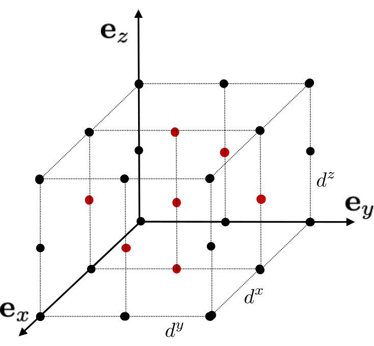
Fig. 1: Sensing an uniform array to obtain ddD-AD antenna configurations.

II-C Arbitrary array deployments

Many antenna deployments, particularly those using cubic or cylindrical geometries, [18, 19], cannot be described, in terms of their associated steering vectors, following the regular structural property mentioned in Section II-B. In the following we refer to such types of AD (AD) as an 33D-AD array.

Given any arbitrary 33D-AD array, the associated steering vector 𝐫N​(𝗳){\mathbf{r}}_{{N}}\left({\boldsymbol{\mathsf{f}}}\right), even though not characterized by any regular structure, can be obtained starting from an encompassing steering vector of a virtual 33D-UD as follows. Let 𝖷​δx{{{\mathsf{X}}}}\delta^{x}, 𝖸​δy{{{\mathsf{Y}}}}\delta^{y} and 𝖹​δz{{{\mathsf{Z}}}}\delta^{z} be the maximum normalized antenna coordinates along the directions of the 33D-AD array, where here δx\delta^{x}, δy\delta^{y}, δz\delta^{z} represents the minimum normalized spacing between the array elements in each direction. Next, consider the virtual 33D-UD with 𝗡¯=[𝖷¯,𝖸¯,𝖹¯]{\bar{\boldsymbol{\mathsf{N}}}}=[\bar{{{\mathsf{X}}}},\bar{{{\mathsf{Y}}}},\bar{{{\mathsf{Z}}}}] elements, encompassing the 33D-AD array, such that 𝖷¯≥𝖷\bar{{{\mathsf{X}}}}\geq{{{\mathsf{X}}}}, 𝖸¯≥𝖸\bar{{{\mathsf{Y}}}}\geq{{{\mathsf{Y}}}} and 𝖹¯≥𝖹\bar{{{\mathsf{Z}}}}\geq{{{\mathsf{Z}}}} and N¯=𝖷¯​𝖸¯​𝖹¯≥N\bar{N}=\bar{{{\mathsf{X}}}}\bar{{{\mathsf{Y}}}}\bar{{{\mathsf{Z}}}}\geq N, with associated steering vector 𝐫𝗡¯​(𝗳){\mathbf{r}}_{{\bar{\boldsymbol{\mathsf{N}}}}}\left({\boldsymbol{\mathsf{f}}}\right):

𝐫𝗡¯​(𝗳)=𝐫𝖷¯​(fx)⊗𝐫𝖸¯​(fy)⊗𝐫𝖹¯​(fz).{\mathbf{r}}_{\bar{{\boldsymbol{\mathsf{N}}}}}\left({\boldsymbol{\mathsf{f}}}\right)={\mathbf{r}}_{\bar{{{\mathsf{X}}}}}(f^{x})\otimes{\mathbf{r}}_{\bar{{{\mathsf{Y}}}}}(f^{y})\otimes{\mathbf{r}}_{\bar{{{\mathsf{Z}}}}}(f^{z}). (3)

Then, 𝐫N​(𝗳){\mathbf{r}}_{{N}}\left({\boldsymbol{\mathsf{f}}}\right) can be obtained starting from 𝐫𝗡¯​(𝗳){\mathbf{r}}_{{\bar{\boldsymbol{\mathsf{N}}}}}\left({\boldsymbol{\mathsf{f}}}\right) using a binary sensing matrix 𝐀∈{0,1}N×N¯{\mathbf{A}}\in\{0,1\}^{N\times\bar{N}}, which effectively removes some elements from 𝐫𝗡¯​(𝗳){\mathbf{r}}_{\bar{\boldsymbol{\mathsf{N}}}}\left({\boldsymbol{\mathsf{f}}}\right) (see Fig. 1 and Fig. 1(a)), as: 11 1 Note that 𝐫N​(𝗳){\mathbf{r}}_{{N}}\left({\boldsymbol{\mathsf{f}}}\right) refers to a steering vector of dimension NN without any specific structure, while 𝐫𝗡​(𝗳){\mathbf{r}}_{{\boldsymbol{\mathsf{N}}}}\left({\boldsymbol{\mathsf{f}}}\right) and 𝐫𝗡¯​(𝗳){\mathbf{r}}_{\bar{{\boldsymbol{\mathsf{N}}}}}\left({\boldsymbol{\mathsf{f}}}\right) represent uniform arrays with a deployment respectively given by 𝗡=[𝖷,𝖸,𝖹]{\boldsymbol{\mathsf{N}}}=[{{\mathsf{X}}},{{\mathsf{Y}}},{{\mathsf{Z}}}] and 𝗡¯=[𝖷¯,𝖸¯,𝖹¯]{\bar{\boldsymbol{\mathsf{N}}}}=[\bar{{{\mathsf{X}}}},\bar{{{\mathsf{Y}}}},\bar{{{\mathsf{Z}}}}] elements.

𝐫N​(𝗳)=𝐀𝐫𝗡¯​(𝗳){\mathbf{r}}_{N}\left({\boldsymbol{\mathsf{f}}}\right)={\mathbf{A}}{\mathbf{r}}_{\bar{{\boldsymbol{\mathsf{N}}}}}\left({\boldsymbol{\mathsf{f}}}\right) (4)

with 𝐀{\mathbf{A}} being a fat matrix with elements ai​j=0a_{ij}=0 if component j∈[N¯]j\in[\bar{N}] in the generating virtual 33D-UD array is not included as component i∈[N]i\in[N] in the 33D-AD array, and ai​j=1a_{ij}=1 otherwise. Note that in order to ensure that the sensing matrix removes elements from the 33D-UD and that one particular element in the 33D-UD is not considered more than once in the 33D-AD the sensing matrix 𝐀∈{0,1}N×N¯{\mathbf{A}}\in\{0,1\}^{N\times\bar{N}} should meet both following conditions 𝐀𝟏N¯=𝟏N{\mathbf{A}}\mathbf{1}_{\bar{N}}=\mathbf{1}_{N} and 𝐀⊤​𝟏N=𝟏N¯{\mathbf{A}}^{\top}\mathbf{1}_{N}=\mathbf{1}_{\bar{N}}. This is equivalent to impose that the sensing matrix 𝐀∈{0,1}N×N¯{\mathbf{A}}\in\{0,1\}^{N\times\bar{N}} belongs to the sensing set 𝒜⊂{0,1}N×N¯\mathcal{A}\subset\{0,1\}^{N\times\bar{N}} defined as:

𝒜={𝐀∈{0,1}N×N¯:[𝐈N|𝟎N×(N¯−N)]𝚷,𝚷∈𝒫}\mathcal{A}=\big\{{\mathbf{A}}\in\{0,1\}^{N\times\bar{N}}:\,\big[{\mathbf{I}}_{N}|{\bf 0}_{N\times(\bar{N}-N)}\big]{\bf\Pi},\,{\bf\Pi}\in\mathcal{P}\big\} (5)

with 𝒫\mathcal{P} the set of all N¯×N¯\bar{N}\times\bar{N} permutation matrices, and N≤𝖷¯​𝖸¯​𝖹¯=N¯N\leq\bar{{{\mathsf{X}}}}\bar{{{\mathsf{Y}}}}\bar{{{\mathsf{Z}}}}=\bar{N}. Each 33D-AD array can be then described using the associated virtual 33D-UD array and sensing matrix 𝐀{\mathbf{A}}. Note that there are multiple pairs of virtual 33D-UD array and sensing matrix 𝐀{\mathbf{A}} that can be associated to a given 33D-AD array.

Remark 1

Note that the ordering of the Kronecker product in (3), induces, via the 33D-UD steering vector 𝐫𝗡¯{\mathbf{r}}_{\bar{{\boldsymbol{\mathsf{N}}}}}, an indexing of the virtual array antenna elements. Such Kronecker ordering is arbitrary and it will be in the following properly chosen to guarantee the maximum system capability in terms of number of resolvable directions 𝐤{\mathbf{k}}. In the following, to refer to the Kronecker ordering given in (3) we use the notation 𝖹¯→𝖸¯→𝖷¯\bar{{{\mathsf{Z}}}}\to\bar{{{\mathsf{Y}}}}\to\bar{{{\mathsf{X}}}}.

III Gridless parameter extraction

Starting from an arbitrary ddD-AD array with d≤3d\leq 3 and its associated general steering vector structure described in Sec. II-C, equations (3)-(4), in this section, we focus on the problem of extracting key multi–dimensional propagation parameters, such as AoA, from the signal received at the antennas elements of the ddD-AD array. Specifically, given a ddD-AD array, under the assumption of KK multiple sources incident on the array from KK AoAs (or equivalently KK local scatters reflecting the impinging incoming signal from KK AoDs), the received signal, measured at the antennas elements, 𝐲∈ℂN{\mathbf{y}}\in{\mathbb{C}}^{N}, can be written as:

𝐲=𝐀𝐑𝗡¯(𝗳1:K⋆)𝐮⋆+𝐰=𝐀𝐬⋆+𝐰,\displaystyle{\mathbf{y}}={\mathbf{A}}{\mathbf{R}}_{\bar{{\boldsymbol{\mathsf{N}}}}}\left({\boldsymbol{\mathsf{f}}}^{\star}_{1:K}\right){\mathbf{u}}^{\star}+{\mathbf{w}}={\mathbf{A}}{\mathbf{s}}^{\star}+{\mathbf{w}}, (6)

where 𝐀∈𝒜{\mathbf{A}}\in\mathcal{A} and 𝐑𝗡¯(𝗳1:K⋆){\mathbf{R}}_{\bar{{\boldsymbol{\mathsf{N}}}}}\left({\boldsymbol{\mathsf{f}}}^{\star}_{1:K}\right)==[𝐫𝗡¯​(𝗳1⋆),…,𝐫𝗡¯​(𝗳K⋆)]∈ℂN¯×K\left[{\mathbf{r}}_{\bar{{\boldsymbol{\mathsf{N}}}}}({\boldsymbol{\mathsf{f}}}^{\star}_{1}),\dots,{\mathbf{r}}_{\bar{{\boldsymbol{\mathsf{N}}}}}({\boldsymbol{\mathsf{f}}}^{\star}_{K})\right]\in{\mathbb{C}}^{\bar{N}\times K} are, respectively, the sensing matrix and the steering vector matrix of the encompassing virtual 33D-UD associated to the ddD-AD array as defined in Sec. II-C, 𝐮⋆=[u1⋆,…,uK⋆]∈ℂK{\mathbf{u}}^{\star}=\left[u^{\star}_{1},\dots,u^{\star}_{K}\right]\in{\mathbb{C}}^{K} is the unknown incoming signal vector incident on the array from the KK AoAs, and 𝐰∈ℂN{\mathbf{w}}\in{\mathbb{C}}^{N} is the AWGN (AWGN) noise vector whose elements are independent with zero mean and variance σ2\sigma^{2}.

The objective is to retrieve from the measurement 𝐲∈ℂN{\mathbf{y}}\in{\mathbb{C}}^{N}, in both noiseless (i.e. 𝐰=𝟎N×1{\mathbf{w}}=\mathbf{0}_{N\times 1}) and noisy scenarios (i.e 𝐰≠𝟎N×1{\mathbf{w}}\neq\mathbf{0}_{N\times 1}), the KK–scatter vector 𝐬⋆{\mathbf{s}}^{\star}, the number of sources/scatters, KK, and the associated set of frequencies, 𝗳1:K⋆={𝗳1⋆,𝗳2⋆…,𝗳K⋆}{\boldsymbol{\mathsf{f}}}^{\star}_{1:K}=\left\{{\boldsymbol{\mathsf{f}}}^{\star}_{1},{\boldsymbol{\mathsf{f}}}^{\star}_{2}\dots,{\boldsymbol{\mathsf{f}}}^{\star}_{K}\right\} that characterizes the ddD AoAs of each source/scatter, with 𝗳k⋆∈𝕋d{\boldsymbol{\mathsf{f}}}^{\star}_{k}\in{\mathbb{T}}^{d} and d≤3d\leq 3. All our frequency recovery conditions are derived under the following assumption:

Assumption 1

The ddD frequency vectors, 𝗳k⋆{\boldsymbol{\mathsf{f}}}^{\star}_{k} with k∈[K]k\in[K], associated to the ddD AoAs of the KK sources/scatters are modeled as independent and identically distributed random vectors whose components are independent and uniformly distributed on [0,1)[0,1), i.e. fkα⋆∼𝒰[0,1)f^{\alpha\star}_{k}\sim\mathcal{U}[0,1), for k∈[K]k\in[K], and α∈{x,y,z}\alpha\in\{x,y,z\}.

Note that, given our work’s application scenario, this assumption is not restrictive. In fact, in wireless propagation environments, sources/scatters are typically modeled to be uniformly random placed in the surroundings of the receiver.

Furthermore, even though the derivations of the frequency recovery conditions are conducted for d≤3d\leq 3 given the application scenario of our work, they are applicable also to d>3d>3.

III-A Signal and frequency recovery in noiseless scenarios

III-A1 Problem statement and previous results

In this section, we focus on the noiseless setting, i.e:

𝐲=𝐀𝐑𝗡¯(𝗳1:K⋆)𝐮⋆=𝐀𝐬⋆,{\mathbf{y}}={\mathbf{A}}{\mathbf{R}}_{\bar{{\boldsymbol{\mathsf{N}}}}}\left({\boldsymbol{\mathsf{f}}}^{\star}_{1:K}\right){\mathbf{u}}^{\star}={\mathbf{A}}{\mathbf{s}}^{\star}, (7)

with 𝐀∈𝒜⊂ℂN×N¯{\mathbf{A}}\in\mathcal{A}\subset{\mathbb{C}}^{N\times\bar{N}}. As already stated our objective is to retrieve 𝐬⋆{\mathbf{s}}^{\star}, KK, and 𝗳⋆1:K{\boldsymbol{\mathsf{f}}}^{\star}_{1:K}. As first step, let us provide the following definitions.

Definition 1

Given a N¯\bar{N}-dimensional vector 𝐬{\mathbf{s}}, the ℓ0\ell_{0} AN (ℓ0\ell_{0}-AN) of 𝐬{\mathbf{s}} in ℛ={𝐫𝗡¯​(𝗳):𝗳∈𝕋d}\mathcal{R}=\left\{{\mathbf{r}}_{\bar{{\boldsymbol{\mathsf{N}}}}}({\boldsymbol{\mathsf{f}}}):{\boldsymbol{\mathsf{f}}}\in{\mathbb{T}}^{d}\right\} is defined as ‖𝐬‖ℛ,0=inf𝗳k∈𝕋d,uk∈ℂ{K:𝐬=∑k=1Kuk​𝐫𝗡¯​(𝗳k)}.\left\|{\mathbf{s}}\right\|_{\mathcal{R},0}=\inf_{{\boldsymbol{\mathsf{f}}}_{k}\in{\mathbb{T}}^{d},u_{k}\in{\mathbb{C}}}\bigg\{K:\,\,{\mathbf{s}}=\sum_{k=1}^{K}u_{k}{\mathbf{r}}_{\bar{{\boldsymbol{\mathsf{N}}}}}\left({\boldsymbol{\mathsf{f}}}_{k}\right)\bigg\}. □\square

Definition 2

A KK–scatter vector 𝐬{\mathbf{s}} is defined as a vector whose atomic ℓ0\ell_{0} norm is equal to KK. □\square

It is well known that for a given measurement 𝐲{\mathbf{y}} and a given sensing matrix 𝐀∈𝒜{\mathbf{A}}\in\mathcal{A} as in (5), the KK–scatter vector 𝐬⋆=𝐑𝗡¯(𝗳1:K⋆)𝐮⋆{\mathbf{s}}^{\star}={\mathbf{R}}_{\bar{{\boldsymbol{\mathsf{N}}}}}\left({\boldsymbol{\mathsf{f}}}^{\star}_{1:K}\right){\mathbf{u}}^{\star} can be reconstructed, from the noiseless measurement 𝐲{\mathbf{y}} in (7), as the unique solution of:

min𝐬∈ℂN¯​‖𝐬‖ℛ,0s.t.𝐲=𝐀𝐬\underset{{\mathbf{s}}\in{\mathbb{C}}^{\bar{N}}}{\min}\left\|{\mathbf{s}}\right\|_{\mathcal{R},0}\quad{\rm s.t.}\quad{\mathbf{y}}={\mathbf{A}}{\mathbf{s}} (P.1)

if 𝐀𝐑𝗡¯(𝗳1:2​K⋆){\mathbf{A}}{\mathbf{R}}_{\bar{{\boldsymbol{\mathsf{N}}}}}\left({\boldsymbol{\mathsf{f}}}^{\star}_{1:2K}\right) is injective as a map from ℂ2​K→ℂN{\mathbb{C}}^{2K}\to{\mathbb{C}}^{N}. For the problem of identifying the frequencies, 𝗳⋆1:K{\boldsymbol{\mathsf{f}}}^{\star}_{1:K}, associated to 𝐬⋆{\mathbf{s}}^{\star}, several methods have been proposed in literature [6, 8, 9, 11, 12, 14]. In the following we focus on the so-called gridless approaches [8, 14]. The gridless approach for d=1d=1 is based on the Carathéodory-Fejér theorem. Such approach and the associated Carathéodory-Fejér theorem has been recently generalized to the case of d>1d>1 in [14] by introducing a PSD dd-Level Toeplitz (dd-LT) matrix, whose definition is provided in the following for the specific case of d=3d=3.

Definition 3

Let d=3d=3. A N¯×N¯\bar{N}\times\bar{N} matrix 𝐕∈ℂN¯×N¯{\mathbf{V}}\in{\mathbb{C}}^{\bar{N}\times\bar{N}} is a dd-Level Toeplitz (dd-LT) matrix with nesting ordering 𝖹¯→𝖸¯→𝖷¯\bar{{{\mathsf{Z}}}}\to\bar{{{\mathsf{Y}}}}\to\bar{{{\mathsf{X}}}} if it is a 𝖷¯×𝖷¯\bar{{{\mathsf{X}}}}\times\bar{{{\mathsf{X}}}} block Hermitian Toeplitz matrix defined as 𝐕=𝐕𝗫¯​𝗬¯​𝗭¯{\mathbf{V}}={\mathbf{V}}_{\bar{{\boldsymbol{\mathsf{X}}}}\bar{{\boldsymbol{\mathsf{Y}}}}\bar{{\boldsymbol{\mathsf{Z}}}}} in (8).(a). Furthermore, the 𝖸¯​𝖹¯×𝖸¯​𝖹¯\bar{{{\mathsf{Y}}}}\bar{{{\mathsf{Z}}}}\times\bar{{{\mathsf{Y}}}}\bar{{{\mathsf{Z}}}}-dimensional generic block 𝐕𝖺​𝗬¯​𝗭¯{\mathbf{V}}_{{\mathsf{a}}\bar{{\boldsymbol{\mathsf{Y}}}}\bar{{\boldsymbol{\mathsf{Z}}}}} with −𝖷¯+1≤𝖺≤𝖷¯−1-\bar{{{\mathsf{X}}}}+1\leq{\mathsf{a}}\leq\bar{{{\mathsf{X}}}}-1 is a 𝖸¯×𝖸¯\bar{{{\mathsf{Y}}}}\times\bar{{{\mathsf{Y}}}} block Hermitian Toeplitz matrix of the form given in (8).(b) such that 𝐕𝖺​𝗬¯​𝗭¯=𝐕−𝖺​𝗬¯​𝗭¯†{\mathbf{V}}_{{\mathsf{a}}\bar{{\boldsymbol{\mathsf{Y}}}}\bar{{\boldsymbol{\mathsf{Z}}}}}={\mathbf{V}}_{-{\mathsf{a}}\bar{{\boldsymbol{\mathsf{Y}}}}\bar{{\boldsymbol{\mathsf{Z}}}}}^{\dagger}. Finally, the generic block 𝐕𝖺𝖻​𝗭¯{\mathbf{V}}_{{\mathsf{a}}{\mathsf{b}}\bar{{\boldsymbol{\mathsf{Z}}}}} with −𝖷¯+1≤𝖺≤𝖷¯−1-\bar{{{\mathsf{X}}}}+1\leq{\mathsf{a}}\leq\bar{{{\mathsf{X}}}}-1 and −𝖸¯+1≤𝖻≤𝖸¯−1-\bar{{{\mathsf{Y}}}}+1\leq{\mathsf{b}}\leq\bar{{{\mathsf{Y}}}}-1 is a 𝖹¯×𝖹¯\bar{{{\mathsf{Z}}}}\times\bar{{{\mathsf{Z}}}} Toeplitz matrix given in (8).(c) such that 𝐕𝖺𝖻​𝗭¯=𝐕−𝖺−𝖻​𝗭¯†{\mathbf{V}}_{{\mathsf{a}}{\mathsf{b}}\bar{{\boldsymbol{\mathsf{Z}}}}}={\mathbf{V}}_{-{\mathsf{a}}-{\mathsf{b}}\bar{{\boldsymbol{\mathsf{Z}}}}}^{\dagger}, and defined from vector 𝐯=[v𝖺𝖻⁡(−𝖹¯+1),…,v𝖺𝖻⁡(𝖹¯−1)]∈ℂ(2​𝖹¯−1){\mathbf{v}}=\left[v_{{\mathsf{a}}{\mathsf{b}}(-\bar{{{\mathsf{Z}}}}+1)},\dots,v_{{\mathsf{a}}{\mathsf{b}}(\bar{{{\mathsf{Z}}}}-1)}\right]\in{\mathbb{C}}^{(2\bar{{{\mathsf{Z}}}}-1)} with v𝖺𝖻𝖼=v−𝖺−𝖻−𝖼†v_{{\mathsf{a}}{\mathsf{b}}{\mathsf{c}}}=v_{-{\mathsf{a}}-{\mathsf{b}}-{\mathsf{c}}}^{\dagger} for −𝖷¯+1≤𝖺≤𝖷¯−1-\bar{{{\mathsf{X}}}}+1\leq{\mathsf{a}}\leq\bar{{{\mathsf{X}}}}-1, −𝖸¯+1≤𝖻≤𝖸¯−1-\bar{{{\mathsf{Y}}}}+1\leq{\mathsf{b}}\leq\bar{{{\mathsf{Y}}}}-1 and −𝖹¯+1≤𝖼≤𝖹¯−1-\bar{{{\mathsf{Z}}}}+1\leq{\mathsf{c}}\leq\bar{{{\mathsf{Z}}}}-1.

𝐕𝗫¯​𝗬¯​𝗭¯=[𝐕0​𝗬¯​𝗭¯…𝐕(𝖷¯−1)​𝗬¯​𝗭¯𝐕(−1)​𝗬¯​𝗭¯…𝐕(𝖷¯−2)​𝗬¯​𝗭¯𝐕(−𝖷¯+1)​𝗬¯​𝗭¯…𝐕0​𝗬¯​𝗭¯]𝐕𝖺​𝗬¯​𝗭¯=[𝐕𝖺​0​𝗭¯…𝐕𝖺⁡(𝖸¯−1)​𝗭¯𝐕𝖺⁡(−1)​𝗭¯…𝐕𝖺⁡(𝖸¯−2)​𝗭¯𝐕𝖺⁡(−𝖸¯+1)​𝗭¯…𝐕𝖺​0​𝗭¯]𝐕𝖺𝖻​𝗭¯=[v𝖺𝖻​0…v𝖺𝖻⁡(𝖹¯−1)v𝖺𝖻⁡(−1)…v𝖺𝖻⁡(𝖹¯−2)v𝖺𝖻⁡(−𝖹¯+1)…v𝖺𝖻​0](a)(b)(c)\begin{array}[]{cccc}\!\!\!\!\!\!{\mathbf{V}}_{\bar{{\boldsymbol{\mathsf{X}}}}\bar{{\boldsymbol{\mathsf{Y}}}}\bar{{\boldsymbol{\mathsf{Z}}}}}=\begin{bmatrix}{\mathbf{V}}_{0\bar{{\boldsymbol{\mathsf{Y}}}}\bar{{\boldsymbol{\mathsf{Z}}}}}&\dots&{\mathbf{V}}_{(\bar{{{\mathsf{X}}}}-1)\bar{{\boldsymbol{\mathsf{Y}}}}\bar{{\boldsymbol{\mathsf{Z}}}}}\\ {\mathbf{V}}_{(-1)\bar{{\boldsymbol{\mathsf{Y}}}}\bar{{\boldsymbol{\mathsf{Z}}}}}&\dots&{\mathbf{V}}_{(\bar{{{\mathsf{X}}}}-2)\bar{{\boldsymbol{\mathsf{Y}}}}\bar{{\boldsymbol{\mathsf{Z}}}}}\\ \vdots&&\vdots\\ {\mathbf{V}}_{(-\bar{{{\mathsf{X}}}}+1)\bar{{\boldsymbol{\mathsf{Y}}}}\bar{{\boldsymbol{\mathsf{Z}}}}}&\dots&{\mathbf{V}}_{0\bar{{\boldsymbol{\mathsf{Y}}}}\bar{{\boldsymbol{\mathsf{Z}}}}}\\ \end{bmatrix}&{\mathbf{V}}_{{\mathsf{a}}\bar{{\boldsymbol{\mathsf{Y}}}}\bar{{\boldsymbol{\mathsf{Z}}}}}=\begin{bmatrix}{\mathbf{V}}_{{\mathsf{a}}0\bar{{\boldsymbol{\mathsf{Z}}}}}&\dots&{\mathbf{V}}_{{\mathsf{a}}(\bar{{{\mathsf{Y}}}}-1)\bar{{\boldsymbol{\mathsf{Z}}}}}\\ {\mathbf{V}}_{{\mathsf{a}}(-1)\bar{{\boldsymbol{\mathsf{Z}}}}}&\dots&{\mathbf{V}}_{{\mathsf{a}}(\bar{{{\mathsf{Y}}}}-2)\bar{{\boldsymbol{\mathsf{Z}}}}}\\ \vdots&&\vdots\\ {\mathbf{V}}_{{\mathsf{a}}(-\bar{{{\mathsf{Y}}}}+1)\bar{{\boldsymbol{\mathsf{Z}}}}}&\dots&{\mathbf{V}}_{{\mathsf{a}}0\bar{{\boldsymbol{\mathsf{Z}}}}}\\ \end{bmatrix}&{\mathbf{V}}_{{\mathsf{a}}{\mathsf{b}}\bar{{\boldsymbol{\mathsf{Z}}}}}=\begin{bmatrix}v_{{\mathsf{a}}{\mathsf{b}}0}&\dots&v_{{\mathsf{a}}{\mathsf{b}}(\bar{{{\mathsf{Z}}}}-1)}\\ v_{{\mathsf{a}}{\mathsf{b}}(-1)}&\dots&v_{{\mathsf{a}}{\mathsf{b}}(\bar{{{\mathsf{Z}}}}-2)}\\ \vdots&&\vdots\\ v_{{\mathsf{a}}{\mathsf{b}}(-\bar{{{\mathsf{Z}}}}+1)}&\dots&v_{{\mathsf{a}}{\mathsf{b}}0}\\ \end{bmatrix}\\ \hskip 8.50012pt\hskip 8.50012pt(a)&\hskip 8.50012pt\hskip 8.50012pt(b)&\hskip 8.50012pt\hskip 8.50012pt(c)\end{array} (8)

For d=2d=2, we define a dd-LT matrix using (8).(b) and (8).(c) by fixing 𝖷¯=1\bar{{{\mathsf{X}}}}=1 so that 𝖺=0{\mathsf{a}}=0 and 𝐕=𝐕0​𝗬¯​𝗭¯{\mathbf{V}}={\mathbf{V}}_{0\bar{{\boldsymbol{\mathsf{Y}}}}\bar{{\boldsymbol{\mathsf{Z}}}}}. Analogously, for d=1d=1, we define a dd-LT matrix from (8).(c) by fixing 𝖷¯=1\bar{{{\mathsf{X}}}}=1 and 𝖸¯=1\bar{{{\mathsf{Y}}}}=1 so that 𝖺=𝖻=0{\mathsf{a}}={\mathsf{b}}=0 and 𝐕=𝐕00​𝗭¯{\mathbf{V}}={\mathbf{V}}_{00\bar{{\boldsymbol{\mathsf{Z}}}}}. □\square

We further introduce the following definition:

Definition 4

Given a N¯×N¯\bar{N}\times\bar{N} 33-LT matrix 𝐕{\mathbf{V}} with nesting ordering 𝖹¯→𝖸¯→𝖷¯\bar{{{\mathsf{Z}}}}\to\bar{{{\mathsf{Y}}}}\to\bar{{{\mathsf{X}}}}, we say that 𝐕{\mathbf{V}} has a canonical ordered structure (or equivalently 𝐕{\mathbf{V}} is a canonical dd-LT matrix) if there is a descending ordering in the component dimensions i.e. 𝖷¯≤𝖸¯≤𝖹¯\bar{{{\mathsf{X}}}}\leq\bar{{{\mathsf{Y}}}}\leq\bar{{{\mathsf{Z}}}}. □\square

Remark 2

There is an interesting connection, that we will later explore, between the Kronecker ordering of a steering vector and the nesting ordering of a 33-LT matrix. Given a set of KK steering vectors 𝐫𝗡¯​(𝗳k){\mathbf{r}}_{\bar{{\boldsymbol{\mathsf{N}}}}}({\boldsymbol{\mathsf{f}}}_{k}) with k∈[K]k\in[K] with Kronecker ordering 𝖹¯→𝖸¯→𝖷¯\bar{{{\mathsf{Z}}}}\to\bar{{{\mathsf{Y}}}}\to\bar{{{\mathsf{X}}}} (see Remark 1), the N¯×N¯{\bar{N}}\times{\bar{N}} matrix defined as 𝐕=∑k=1Kpk​𝐫𝗡¯​(𝗳k)​𝐫𝗡¯​(𝗳k)†{\mathbf{V}}=\sum_{k=1}^{K}p_{k}{\mathbf{r}}_{\bar{{\boldsymbol{\mathsf{N}}}}}({\boldsymbol{\mathsf{f}}}_{k}){\mathbf{r}}_{\bar{{\boldsymbol{\mathsf{N}}}}}({\boldsymbol{\mathsf{f}}}_{k})^{\dagger} is a PSD 33-LT matrix with nesting ordering 𝖹¯→𝖸¯→𝖷¯\bar{{{\mathsf{Z}}}}\to\bar{{{\mathsf{Y}}}}\to\bar{{{\mathsf{X}}}}.

Using the previous definitions, we now overview some previous results. In [14, Theorem 3] the authors show that given a 33D-UD array with 𝗡=[𝖷,𝖸,𝖹]{\boldsymbol{\mathsf{N}}}=[{{\mathsf{X}}},{{\mathsf{Y}}},{{\mathsf{Z}}}] elements, and its associated pair of sensing matrix 𝐀𝖴{\mathbf{A}}_{\sf{U}} and virtual 33D-UD array of 𝗡¯=[𝖷¯,𝖸¯,𝖹¯]{\bar{\boldsymbol{\mathsf{N}}}}=[\bar{{{\mathsf{X}}}},\bar{{{\mathsf{Y}}}},\bar{{{\mathsf{Z}}}}] elements, the recived signal 𝐬⋆{\mathbf{s}}^{\star} (the incoming signal 𝐮⋆{\mathbf{u}}^{\star}) and its associated frequencies 𝗳⋆1:K{\boldsymbol{\mathsf{f}}}^{\star}_{1:K} can be uniquely and perfectly reconstructed from the noiseless measurement 𝐲{\mathbf{y}} in (7), solving the following rank\rank minimization problem [14, Theorem 3, Remark 4]:

minr,𝐬∈ℂN¯,𝐒𝗫¯​𝗬¯​𝗭¯\displaystyle\min_{r,{\mathbf{s}}\in{\mathbb{C}}^{\bar{N}},{\mathbf{S}}_{\bar{{\boldsymbol{\mathsf{X}}}}\bar{{\boldsymbol{\mathsf{Y}}}}\bar{{\boldsymbol{\mathsf{Z}}}}}} rank⁡{𝐒𝗫¯​𝗬¯​𝗭¯}s.t.\displaystyle\rank\left\{{\mathbf{S}}_{\bar{{\boldsymbol{\mathsf{X}}}}\bar{{\boldsymbol{\mathsf{Y}}}}\bar{{\boldsymbol{\mathsf{Z}}}}}\right\}\quad\quad\quad{\rm s.t.}\quad [𝐒𝗫¯​𝗬¯​𝗭¯𝐬𝐬†r]⪰0,\displaystyle\begin{bmatrix}{\mathbf{S}}_{\bar{{\boldsymbol{\mathsf{X}}}}\bar{{\boldsymbol{\mathsf{Y}}}}\bar{{\boldsymbol{\mathsf{Z}}}}}&{\mathbf{s}}\\ {\mathbf{s}}^{\dagger}&r\end{bmatrix}\succeq 0, 𝐀𝖴​𝐬=𝐲,\displaystyle{\displaystyle\mathbf{A}}_{\sf{U}}{\mathbf{s}}={\mathbf{y}}, (P.2)

if K<min⁡{𝖷¯,𝖸¯,𝖹¯}K<\min\left\{\bar{{{\mathsf{X}}}},\bar{{{\mathsf{Y}}}},\bar{{{\mathsf{Z}}}}\right\}. In (P.2) 𝐒𝗫¯​𝗬¯​𝗭¯{\mathbf{S}}_{\bar{{\boldsymbol{\mathsf{X}}}}\bar{{\boldsymbol{\mathsf{Y}}}}\bar{{\boldsymbol{\mathsf{Z}}}}} is a PSD dd-LT matrix with arbitrary nesting order and 𝐀𝖴=[𝐈N|𝟎N×(N¯−N)]​𝚷𝖴{\mathbf{A}}_{\sf{U}}=\big[{\mathbf{I}}_{N}|{\bf 0}_{N\times(\bar{N}-N)}\big]{\bf{\Pi}_{\sf{U}}} with 𝚷𝖴{\bf{\Pi}_{\sf{U}}} a proper permutation matrix such that only the first 𝖷≤𝖷¯{{\mathsf{X}}}\leq\bar{{{\mathsf{X}}}}, 𝖸≤𝖸¯{{\mathsf{Y}}}\leq\bar{{{\mathsf{Y}}}}, and 𝖹≤𝖹¯{{\mathsf{Z}}}\leq\bar{{{\mathsf{Z}}}} antennas are sensed. However, the results in [14, Theorem 3] only hold for 33D-UD arrays and rely (for the frequency recovery) on the uniqueness of the Vandermonde decomposition of the resulting min-rank PSD dd-LT matrix, 𝐒𝗫¯​𝗬¯​𝗭¯∘{\mathbf{S}}^{\circ}_{\bar{{\boldsymbol{\mathsf{X}}}}\bar{{\boldsymbol{\mathsf{Y}}}}\bar{{\boldsymbol{\mathsf{Z}}}}}, which can only be guaranteed if rank⁡{𝐒𝗫¯​𝗬¯​𝗭¯∘}<min⁡{𝖷¯,𝖸¯,𝖹¯}\rank\left\{{\mathbf{S}}^{\circ}_{\bar{{\boldsymbol{\mathsf{X}}}}\bar{{\boldsymbol{\mathsf{Y}}}}\bar{{\boldsymbol{\mathsf{Z}}}}}\right\}<\min\left\{\bar{{{\mathsf{X}}}},\bar{{{\mathsf{Y}}}},\bar{{{\mathsf{Z}}}}\right\} (see [14, Theorem 1]).

In the next section, we derive recovery results for arbitrary ddD-AD arrays and, exploiting the structure of our problem, we are able to reformulate [14, Theorem 1] and [14, Theorem 3] and effectively enlarge the frequency recovery region, under much less restrictive conditions on the rank\rank of a PSD 33-LT matrix and on the dimensions of the virtual array.

III-A2 Main results on recovery conditions

In this section, we provide the exact characterization of the frequency recovery region for arbitrary ddD-AD array, with d≤3d\leq 3 by identifying the conditions on the system parameters that guarantee, from the measurement 𝐲{\mathbf{y}} in (7), perfect and unique recovery of the KK–scatter vector 𝐬⋆{\mathbf{s}}^{\star} and its associated frequencies 𝗳⋆1:K∈𝕋d×K{\boldsymbol{\mathsf{f}}}^{\star}_{1:K}\in{\mathbb{T}}^{d\times K}.

Before stating our main results, let us present the following lemma, which will be used to prove our frequency recovery conditions and which also extends the result provided in [14, Theorem 1], deriving a less restrictive sufficient condition for the uniqueness of the Vandermonde decomposition of a dd-level Toeplitz matrix.

Lemma 1

Let 𝐒∈ℂN¯×N¯{\mathbf{S}}\in{\mathbb{C}}^{\bar{N}\times\bar{N}} be an N¯×N¯\bar{N}\times\bar{N} PSD dd-LT matrix with rank\rank r<max⁡{𝖷¯,𝖸¯,𝖹¯}r<\max\left\{\bar{{{\mathsf{X}}}},\bar{{{\mathsf{Y}}}},\bar{{{\mathsf{Z}}}}\right\}, and with ordered canonical structure (as per Definition 4). Denoting W=max⁡{𝖷¯,𝖸¯,𝖹¯}W=\max\left\{\bar{{{\mathsf{X}}}},\bar{{{\mathsf{Y}}}},\bar{{{\mathsf{Z}}}}\right\}, if the rank\rank of the W×WW\times W upper-left corner22 2 The W×WW\times W upper-left corner of 𝐒{\mathbf{S}}, is the W×WW\times W sub block of 𝐒{\mathbf{S}} obtained considering the first WW rows and the first WW columns of 𝐒{\mathbf{S}}. of 𝐒{\mathbf{S}} also equals rr then 𝐒{\mathbf{S}} can be uniquely decomposed, via Algorithm 1, as 𝐒=𝐑𝗡¯(𝗳1:r)𝐏𝐑𝗡¯†(𝗳1:r),{\mathbf{S}}={\mathbf{R}}_{\bar{{\boldsymbol{\mathsf{N}}}}}\left({\boldsymbol{\mathsf{f}}}_{1:r}\right){\mathbf{P}}{\mathbf{R}}^{\dagger}_{\bar{{\boldsymbol{\mathsf{N}}}}}\left({\boldsymbol{\mathsf{f}}}_{1:r}\right), with 𝗳1:r={𝗳1,𝗳2…,𝗳r}∈𝕋d×r{\boldsymbol{\mathsf{f}}}_{1:r}=\left\{{\boldsymbol{\mathsf{f}}}_{1},{\boldsymbol{\mathsf{f}}}_{2}\dots,{\boldsymbol{\mathsf{f}}}_{{r}}\right\}\in{\mathbb{T}}^{d\times r} being a unique set of frequencies, 𝐑𝗡¯(𝗳1:r)=[𝐫𝗡¯(𝗳1),𝐫𝗡¯(𝗳2),…,𝐫𝗡¯(𝗳r)]∈ℂN¯×r{\mathbf{R}}_{\bar{{\boldsymbol{\mathsf{N}}}}}\left({\boldsymbol{\mathsf{f}}}_{1:r}\right)=\left[{\mathbf{r}}_{\bar{{\boldsymbol{\mathsf{N}}}}}({\boldsymbol{\mathsf{f}}}_{1}),{\mathbf{r}}_{\bar{{\boldsymbol{\mathsf{N}}}}}({\boldsymbol{\mathsf{f}}}_{2}),\dots,{\mathbf{r}}_{\bar{{\boldsymbol{\mathsf{N}}}}}({\boldsymbol{\mathsf{f}}}_{r})\right]\in{\mathbb{C}}^{\bar{N}\times r} being the steering vector matrix associated to the vector frequencies 𝗳1:r{\boldsymbol{\mathsf{f}}}_{1:r}, and 𝐏=diag⁡([p1,…,pr]){\mathbf{P}}=\diag\left([p_{1},\dots,p_{r}]\right), pk∈ℝ+p_{k}\in{\mathbb{R}}^{+} with k∈[r]k\in[r].

Proof:

The proof is given in Appendix A, where in a constructive way we prove existence and consequently uniqueness of the Vandermonde decomposition of 𝐒{\mathbf{S}}. Following the proof we are also able to develop an algorithm (Alg. 1) that can be applied now with less stringent conditions on the rank\rank than in [14]. ∎

Algorithm 1 Algorithm for Lemma 1
1:  Input: 𝐒=𝐒𝗫¯​𝗬¯​𝗭¯{\mathbf{S}}={\mathbf{S}}_{\bar{{\boldsymbol{\mathsf{X}}}}\bar{{\boldsymbol{\mathsf{Y}}}}\bar{{\boldsymbol{\mathsf{Z}}}}} with rank⁡{𝐒𝗫¯​𝗬¯​𝗭¯}=r\rank\{{\mathbf{S}}_{\bar{{\boldsymbol{\mathsf{X}}}}\bar{{\boldsymbol{\mathsf{Y}}}}\bar{{\boldsymbol{\mathsf{Z}}}}}\}=r.Step 1: Decomposing in the 𝖷¯\bar{{{\mathsf{X}}}} dimension
2:  Obtain the Cholesky decomposition of 𝐒𝗫¯​𝗬¯​𝗭¯=𝐂𝖷¯​𝖸¯​𝖹¯​𝐂𝖷¯​𝖸¯​𝖹¯†{\mathbf{S}}_{\bar{{\boldsymbol{\mathsf{X}}}}\bar{{\boldsymbol{\mathsf{Y}}}}\bar{{\boldsymbol{\mathsf{Z}}}}}={\mathbf{C}}_{\bar{{{\mathsf{X}}}}\bar{{{\mathsf{Y}}}}\bar{{{\mathsf{Z}}}}}{\mathbf{C}}_{\bar{{{\mathsf{X}}}}\bar{{{\mathsf{Y}}}}\bar{{{\mathsf{Z}}}}}^{\dagger}.
3:  Split 𝐂𝖷¯​𝖸¯​𝖹¯{\mathbf{C}}_{\bar{{{\mathsf{X}}}}\bar{{{\mathsf{Y}}}}\bar{{{\mathsf{Z}}}}} matrix row-wise in 𝖷¯\bar{{{\mathsf{X}}}} blocks as 𝐂𝖷¯​𝖸¯​𝖹¯=[𝐂0​𝖸¯​𝖹¯†,𝐂1​𝖸¯​𝖹¯†,…,𝐂(𝖷−1)​𝖸¯​𝖹¯†]†{\mathbf{C}}_{\bar{{{\mathsf{X}}}}\bar{{{\mathsf{Y}}}}\bar{{{\mathsf{Z}}}}}=[{\mathbf{C}}_{0\bar{{{\mathsf{Y}}}}\bar{{{\mathsf{Z}}}}}^{\dagger},{\mathbf{C}}_{1\bar{{{\mathsf{Y}}}}\bar{{{\mathsf{Z}}}}}^{\dagger},\dots,{\mathbf{C}}_{({{\mathsf{X}}}-1)\bar{{{\mathsf{Y}}}}\bar{{{\mathsf{Z}}}}}^{\dagger}]^{\dagger}.
4:  if 𝖷¯>1\bar{{{\mathsf{X}}}}>1 then
5:   Find the 𝐔𝖷¯{\mathbf{U}}_{\bar{{{\mathsf{X}}}}} unitary matrix such that [𝐂0​𝖸¯​𝖹¯†,𝐂1​𝖸¯​𝖹¯†,…,𝐂(𝖷−2)​𝖸¯​𝖹¯†]†​𝐔𝖷¯=[𝐂1​𝖸¯​𝖹¯†,𝐂2​𝖸¯​𝖹¯†,…,𝐂(𝖷−1)​𝖸¯​𝖹¯†]†[{\mathbf{C}}_{0\bar{{{\mathsf{Y}}}}\bar{{{\mathsf{Z}}}}}^{\dagger},{\mathbf{C}}_{1\bar{{{\mathsf{Y}}}}\bar{{{\mathsf{Z}}}}}^{\dagger},\dots,{\mathbf{C}}_{({{\mathsf{X}}}-2)\bar{{{\mathsf{Y}}}}\bar{{{\mathsf{Z}}}}}^{\dagger}]^{\dagger}{\mathbf{U}}_{\bar{{{\mathsf{X}}}}}=[{\mathbf{C}}_{1\bar{{{\mathsf{Y}}}}\bar{{{\mathsf{Z}}}}}^{\dagger},{\mathbf{C}}_{2\bar{{{\mathsf{Y}}}}\bar{{{\mathsf{Z}}}}}^{\dagger},\dots,{\mathbf{C}}_{({{\mathsf{X}}}-1)\bar{{{\mathsf{Y}}}}\bar{{{\mathsf{Z}}}}}^{\dagger}]^{\dagger}.
6:   Obtain the eigen-decomposition 𝐔𝖷¯=𝐊𝖷¯​𝐗𝐊𝖷¯†{\mathbf{U}}_{\bar{{{\mathsf{X}}}}}={\mathbf{K}}_{\bar{{{\mathsf{X}}}}}{\mathbf{X}}{\mathbf{K}}_{\bar{{{\mathsf{X}}}}}^{\dagger} and we have that 𝐗=diag⁡(e𝚓​2​π​f1x,…,e𝚓​2​π​frx){\mathbf{X}}=\diag(e^{{\mathtt{j}}2\pi f^{x}_{1}},\dots,e^{{\mathtt{j}}2\pi f^{x}_{r}})
7:  else
8:   Set fkx=0f^{x}_{k}=0 ∀k=[1,…,r]\forall k=[1,\dots,r]
9:  end ifStep 2: Decomposing in the 𝖸¯\bar{{{\mathsf{Y}}}} dimension
10:  Split 𝐂0​𝖸¯​𝖹¯{\mathbf{C}}_{0\bar{{{\mathsf{Y}}}}\bar{{{\mathsf{Z}}}}} matrix row-wise in 𝖸¯\bar{{{\mathsf{Y}}}} blocks as 𝐂0​𝖸¯​𝖹¯=[𝐂00​𝖹¯†,𝐂01​𝖹¯†,…,𝐂0​(𝖸−1)​𝖹¯†]†{\mathbf{C}}_{0\bar{{{\mathsf{Y}}}}\bar{{{\mathsf{Z}}}}}=[{\mathbf{C}}_{00\bar{{{\mathsf{Z}}}}}^{\dagger},{\mathbf{C}}_{01\bar{{{\mathsf{Z}}}}}^{\dagger},\dots,{\mathbf{C}}_{0({{\mathsf{Y}}}-1)\bar{{{\mathsf{Z}}}}}^{\dagger}]^{\dagger}.
11:  if 𝖸¯>1\bar{{{\mathsf{Y}}}}>1 then
12:   Find the 𝐔𝖸¯{\mathbf{U}}_{\bar{{{\mathsf{Y}}}}} unitary matrix such that [𝐂00​𝖹¯†,𝐂01​𝖹¯†,…,𝐂0​(𝖸−2)​𝖹¯†]†​𝐔𝖸¯=[𝐂01​𝖹¯†,𝐂01​𝖹¯†,…,𝐂0​(𝖸−1)​𝖹¯†]†[{\mathbf{C}}_{00\bar{{{\mathsf{Z}}}}}^{\dagger},{\mathbf{C}}_{01\bar{{{\mathsf{Z}}}}}^{\dagger},\dots,{\mathbf{C}}_{0({{\mathsf{Y}}}-2)\bar{{{\mathsf{Z}}}}}^{\dagger}]^{\dagger}{\mathbf{U}}_{\bar{{{\mathsf{Y}}}}}=[{\mathbf{C}}_{01\bar{{{\mathsf{Z}}}}}^{\dagger},{\mathbf{C}}_{01\bar{{{\mathsf{Z}}}}}^{\dagger},\dots,{\mathbf{C}}_{0({{\mathsf{Y}}}-1)\bar{{{\mathsf{Z}}}}}^{\dagger}]^{\dagger}.
13:   Obtain the eigen-decomposition 𝐔𝖸¯=𝐊𝖸¯​𝐘𝐊𝖸¯†{\mathbf{U}}_{\bar{{{\mathsf{Y}}}}}={\mathbf{K}}_{\bar{{{\mathsf{Y}}}}}{\mathbf{Y}}{\mathbf{K}}_{\bar{{{\mathsf{Y}}}}}^{\dagger} and we have that 𝐘=diag⁡(e𝚓​2​π​f1y,…,e𝚓​2​π​fry){\mathbf{Y}}=\diag(e^{{\mathtt{j}}2\pi f^{y}_{1}},\dots,e^{{\mathtt{j}}2\pi f^{y}_{r}})
14:  else
15:   Set fky=0f^{y}_{k}=0 ∀k=[1,…,r]\forall k=[1,\dots,r]
16:  end ifStep 3: Decomposing in the 𝖹¯\bar{{{\mathsf{Z}}}} dimension
17:  Split 𝐂00​𝖹¯{\mathbf{C}}_{00\bar{{{\mathsf{Z}}}}} matrix row-wise and find the 𝐔𝖹¯{\mathbf{U}}_{\bar{{{\mathsf{Z}}}}} unitary matrix such that 𝐂00[0:𝖹¯−2]𝐔𝖹¯=𝐂00[1:𝖹¯−1]{\mathbf{C}}_{00[0:\bar{{{\mathsf{Z}}}}-2]}{\mathbf{U}}_{\bar{{{\mathsf{Z}}}}}={\mathbf{C}}_{00[1:\bar{{{\mathsf{Z}}}}-1]}.
18:  Obtain the eigen-decomposition 𝐔𝖹¯=𝐊𝖹¯​𝐙𝐊𝖹¯†{\mathbf{U}}_{\bar{{{\mathsf{Z}}}}}={\mathbf{K}}_{\bar{{{\mathsf{Z}}}}}{\mathbf{Z}}{\mathbf{K}}_{\bar{{{\mathsf{Z}}}}}^{\dagger} and we have that 𝐙=diag⁡(e𝚓​2​π​f1z,…,e𝚓​2​π​frz){\mathbf{Z}}=\diag(e^{{\mathtt{j}}2\pi f^{z}_{1}},\dots,e^{{\mathtt{j}}2\pi f^{z}_{r}})Step 4: Obtain the set of frequencies 𝖿1:r{\boldsymbol{\mathsf{f}}}_{1:r}
19:  Do the frequency pairing according to [14].
20:  Output: The recovered frequencies 𝗳1:r=[f1:rx⊤f1:ry⊤f1:rz⊤]⊤{\boldsymbol{\mathsf{f}}}_{1:r}=[f^{x\top}_{1:r}f^{y\top}_{1:r}f^{z^{\top}}_{1:r}]^{\top}, the full rank\rank matrix 𝐑𝗡¯(𝗳1:r)=[𝐫𝗡¯(𝗳1),…,𝐫𝗡¯(𝗳r)]{\mathbf{R}}_{\bar{{\boldsymbol{\mathsf{N}}}}}\left({\boldsymbol{\mathsf{f}}}_{1:r}\right)=\left[{\mathbf{r}}_{\bar{{\boldsymbol{\mathsf{N}}}}}({\boldsymbol{\mathsf{f}}}_{1}),\dots,{\mathbf{r}}_{\bar{{\boldsymbol{\mathsf{N}}}}}({\boldsymbol{\mathsf{f}}}_{r})\right] and 𝐏=𝐑𝗡¯𝗀(𝗳1:r)𝐒𝗫¯​𝗬¯​𝗭¯𝐑𝗡¯†𝗀(𝗳1:r){\mathbf{P}}={\mathbf{R}}_{\bar{{\boldsymbol{\mathsf{N}}}}}^{\mathsf{g}}\left({\boldsymbol{\mathsf{f}}}_{1:r}\right){\mathbf{S}}_{\bar{{\boldsymbol{\mathsf{X}}}}\bar{{\boldsymbol{\mathsf{Y}}}}\bar{{\boldsymbol{\mathsf{Z}}}}}{\mathbf{R}}_{\bar{{\boldsymbol{\mathsf{N}}}}}^{\dagger{\mathsf{g}}}\left({\boldsymbol{\mathsf{f}}}_{1:r}\right).

Note that while Lemma 1 is stated for d∈{1,2,3}d\in\{1,2,3\}, it is worth to underline that the result holds even for d>3d>3.

Remark 3

Lemma 1 admits a more general formulation where denoting by 𝐒∈ℂN¯×N¯{{\mathbf{S}}}\in{\mathbb{C}}^{\bar{N}\times\bar{N}} an N¯×N¯\bar{N}\times\bar{N} PSD dd-LT matrix with rank rr, and denoting by WW the dimension of the largest 11-LT upper-left corner of 𝐒{\mathbf{S}}. If the rank\rank of such block also equals rr and r<Wr<W, then 𝐒{\mathbf{S}} admits a unique Vandermonde decomposition.

Remark 4

Lemma 1 shows that while the sufficient condition for the uniqueness of the Vandermonde decomposition (r<min⁡{𝖷¯,𝖸¯,𝖹¯}r<\min\left\{\bar{{{\mathsf{X}}}},\bar{{{\mathsf{Y}}}},\bar{{{\mathsf{Z}}}}\right\}) in [14, Theorem 1] is tight for d=1d=1, this would not hold any more for a PSD dd-LT matrix 𝐒∈ℂN¯×N¯{\mathbf{S}}\in{\mathbb{C}}^{\bar{N}\times\bar{N}} with d≥2d\geq 2. In fact if 𝐒∈ℂN¯×N¯{\mathbf{S}}\in{\mathbb{C}}^{\bar{N}\times\bar{N}} follows Lemma 1 conditions, then a sufficient condition for 𝐒{\mathbf{S}} to admit a unique Vandermonde decomposition is the less restrictive condition r<max⁡{𝖷¯,𝖸¯,𝖹¯}r<\max\left\{\bar{{{\mathsf{X}}}},\bar{{{\mathsf{Y}}}},\bar{{{\mathsf{Z}}}}\right\}, compared to r<min⁡{𝖷¯,𝖸¯,𝖹¯}r<\min\left\{\bar{{{\mathsf{X}}}},\bar{{{\mathsf{Y}}}},\bar{{{\mathsf{Z}}}}\right\} [14, Theorem 1]. This interesting result essentially stems from the fact that the proposed decomposition approach relies on the decomposing the upper-left block matrix in 𝐒{\mathbf{S}}, cf. lines 17 and 18 of Algorithm 1. Therefore, the canonical ordering required in Lemma 1 poses the base to allow the less restrictive condition (r<max⁡{𝖷¯,𝖸¯,𝖹¯}r<\max\left\{\bar{{{\mathsf{X}}}},\bar{{{\mathsf{Y}}}},\bar{{{\mathsf{Z}}}}\right\}) on the uniqueness of the decomposition and hence enlarges the set of PSD dd-LT matrix for which we can guarantee unique decomposition. However, if the ordering does not follow Definition 4, as required in Lemma 1, one has to enforce the condition stated in [14, Theorem 1], i.e. r<min⁡{𝖷¯,𝖸¯,𝖹¯}r<\min\left\{\bar{{{\mathsf{X}}}},\bar{{{\mathsf{Y}}}},\bar{{{\mathsf{Z}}}}\right\}, to ensure the decomposability of the upper-left block matrix. To the best of the authors’ knowledge, the result stated in Lemma 1 is the tightest condition for the uniqueness decomposition of PSD dd-LT matrices in the literature.

In addition to Lemma 1, in order to state our recovery conditions, we also need to provide some few useful definitions and assumptions.

Specifically, in the following, we always consider as Kronecker ordering for the virtual 33D-UD streering vectors 𝖹¯→𝖸¯→𝖷¯\bar{{{\mathsf{Z}}}}\to\bar{{{\mathsf{Y}}}}\to\bar{{{\mathsf{X}}}} and we always assume without loss of generality 𝖷¯≤𝖸¯≤𝖹¯\bar{{{\mathsf{X}}}}\leq\bar{{{\mathsf{Y}}}}\leq\bar{{{\mathsf{Z}}}}. Note that in case this assumption would not initially hold, we can always operate a proper rotation of the Cartesian system (which corresponds to a permutation of the elements of the measurement vector 𝐲{\mathbf{y}}, or a different reading of the antenna elements of the dd-AD). This will ensure that we can always enforce the canonical ordering of Definition 4 on the set of PSD matrices, in the subsequent proposed min\min-rank\rank optimization.

Furthermore, being 𝒜\mathcal{A} the sensing set defined in (5), let us introduce the following definition:

Definition 5

𝒜(K)⊂𝒜\mathcal{A}^{(K)}\subset\mathcal{A} denotes the subset of all binary N×N¯N\times\bar{N} sensing matrices 𝒜\mathcal{A} for which it exists a subset of rows of 𝐀∈𝒜{\mathbf{A}}\in\mathcal{A}, say ℒ⊆[N]{\mathcal{L}\subseteq[N]} with 2​K<|ℒ|≤N2K<|{\mathcal{L}}|\leq N such that:

  • 1.C

    under Assumption 1, 𝐀(ℒ)𝐑𝗡¯(𝗳1:2​K){\mathbf{A}}^{{(\mathcal{L})}}{\mathbf{R}}_{\bar{{\boldsymbol{\mathsf{N}}}}}({\boldsymbol{\mathsf{f}}}_{1:2K}) is injective as map from ℂ2​K→ℂ|ℒ|{\mathbb{C}}^{2K}\to{\mathbb{C}}^{|{\mathcal{L}}|};

  • 2.C

    denoted by 𝗳⋆1:K{\boldsymbol{\mathsf{f}}}^{\star}_{1:K} a set of KK frequencies satisfying Assumption 1 and by 𝗳⋄1:r⋄{\boldsymbol{\mathsf{f}}}^{\diamond}_{1:r^{\diamond}} an arbitrary set of r⋄≤K{r^{\diamond}}\leq K frequencies such that for any k∈[K]k\in[K] and j∈[r⋄]j\in[{r^{\diamond}}], 𝗳j⋄≠𝗳k⋆{\boldsymbol{\mathsf{f}}}^{\diamond}_{j}\neq{\boldsymbol{\mathsf{f}}}^{\star}_{k}, rank{𝐀(ℒ)𝐑𝗡¯(𝗳1:K+r⋄⋆⁣⋄)}=K+rank{𝐀(ℒ)𝐑𝗡¯(𝗳1:r⋄⋄)}\rank\left\{{\mathbf{A}}^{{(\mathcal{L})}}{\mathbf{R}}_{\bar{{\boldsymbol{\mathsf{N}}}}}({{\boldsymbol{\mathsf{f}}}^{\star\diamond}_{1:K+r^{\diamond}}})\right\}=K+\rank\left\{{\mathbf{A}}^{{(\mathcal{L})}}{\mathbf{R}}_{\bar{{\boldsymbol{\mathsf{N}}}}}({{\boldsymbol{\mathsf{f}}}^{\diamond}_{1:{r^{\diamond}}})}\right\}, with 𝗳1:K+r⋄⋆⁣⋄=[𝗳1:K⋆𝗳1:r⋄⋄]{{\boldsymbol{\mathsf{f}}}^{\star\diamond}_{1:K+r^{\diamond}}=[{\boldsymbol{\mathsf{f}}}^{\star}_{1:K}\,{\boldsymbol{\mathsf{f}}}^{\diamond}_{1:r^{\diamond}}]}. □\square

In the following we provide, through Lemma 5 and Lemma 4 (see Appendices C and D), a class of sensing matrices of practical interest in 𝒜(K)\mathcal{A}^{(K)}. Specifically, in Lemma 5 (see Appendix D), we show that, provided that the number of elements in the ddD-AD array is sufficiently large, 𝒜(K)≡𝒜\mathcal{A}^{(K)}\equiv\mathcal{A} with high probability. In Lemma 4 we identify a second class of matrices, say 𝒜𝖼(K)⊂𝒜\mathcal{A}^{(K)}_{{{\mathsf{c}}}}\subset\mathcal{A}, for which we prove that 𝒜𝖼(K)⊂𝒜(K)\mathcal{A}^{(K)}_{{{\mathsf{c}}}}\subset\mathcal{A}^{(K)}. Such class is identified by the so-called well structured  sensing matrices as in the next two definitions:

Definition 6

A permutation matrix 𝚷{\bf\Pi} belongs to the well structured  permutation class 𝒫𝖼\mathcal{P}_{{{\mathsf{c}}}}, and note it as 𝚷𝖼{\bf\Pi}_{{\mathsf{c}}} if:

  • i)

    denoting by ℐ\mathcal{I} the set of indices for the columns of 𝚷𝖼{\bf\Pi}_{{{\mathsf{c}}}} that have a 11 among its first NN rows33 3 Note that ℐ\mathcal{I} identifies the components of the steering vector 𝐫𝗡¯​(𝗳){\mathbf{r}}_{\bar{{\boldsymbol{\mathsf{N}}}}}({\boldsymbol{\mathsf{f}}}) that are going to be sensed., i.e., j∈ℐj\in\mathcal{I} if ∃n∈[N]\exists\,n\in[N] such that πn​j=1{\pi}_{nj}=1,

  • ii)

    denoting by ℐ𝖼⊆ℐ\mathcal{I}_{{{\mathsf{c}}}}\subseteq\mathcal{I} the largest subset of ordered indices in ℐ\mathcal{I} not necessarily consecutive, such that for any arbitrary vector 𝗳=[fx,fy,fz]⊤∈𝕋d{\boldsymbol{\mathsf{f}}}=[f^{x},f^{y},f^{z}]^{\top}\in{\mathbb{T}}^{d}, the N𝖼N_{{{\mathsf{c}}}} dimensional vector containing the elements of 𝐫𝗡¯​(𝗳){\mathbf{r}}_{\bar{{\boldsymbol{\mathsf{N}}}}}({\boldsymbol{\mathsf{f}}}) whose indices belong to ℐ𝖼{\mathcal{I}_{{{\mathsf{c}}}}} can be written as

    𝐫𝗡¯(ℐ𝖼)​(𝗳)=e𝚓​2​π​(Δx​fx+Δy​fy+Δz​fz)​𝐫𝗡𝖼​(𝗳𝖼){\mathbf{r}}^{{(\mathcal{I}_{{{\mathsf{c}}}})}}_{\bar{{\boldsymbol{\mathsf{N}}}}}({\boldsymbol{\mathsf{f}}})=e^{{\mathtt{j}}2\pi{({\mathsf{\Delta}}_{x}f^{x}+{\mathsf{\Delta}}_{y}f^{y}+{\mathsf{\Delta}}_{z}f^{z})}}{\mathbf{r}}_{{{\boldsymbol{\mathsf{N}}}}_{{{\mathsf{c}}}}}({\boldsymbol{\mathsf{f}}}^{{{\mathsf{c}}}}) (9)

    where 𝐫𝗡𝖼​(𝗳𝖼){\mathbf{r}}_{{{\boldsymbol{\mathsf{N}}}}_{{{\mathsf{c}}}}}({\boldsymbol{\mathsf{f}}}^{{{\mathsf{c}}}}) corresponds to a ddD-UD with structure given by 𝗡𝖼=[𝖷𝖼,𝖸𝖼,𝖹𝖼]{\boldsymbol{\mathsf{N}}}_{{\mathsf{c}}}=[{{\mathsf{X}}}_{{\mathsf{c}}},{{\mathsf{Y}}}_{{\mathsf{c}}},{{\mathsf{Z}}}_{{\mathsf{c}}}], and 𝗳𝖼=[ℓx​fx,ℓy​fy,ℓz​fz]⊤{\boldsymbol{\mathsf{f}}}^{{{\mathsf{c}}}}=\left[\ell_{x}f^{x},\ell_{y}f^{y},\ell_{z}f^{z}\right]^{\top} is a dd-dimensional vector with ℓα\ell_{\alpha} a proper positive integer, α∈(x,y,z)\alpha\in(x,y,z), Δx∈[𝖷¯]{{\mathsf{\Delta}}_{x}}\in[{\bar{{{\mathsf{X}}}}}], Δy∈[𝖸¯]{{\mathsf{\Delta}}_{y}}\in[{\bar{{{\mathsf{Y}}}}}], Δz∈[𝖹¯]{{\mathsf{\Delta}}_{z}}\in[{\bar{{{\mathsf{Z}}}}}] and finally S𝖼=𝖷𝖼+𝖸𝖼+𝖹𝖼S_{{{\mathsf{c}}}}={{\mathsf{X}}}_{{\mathsf{c}}}+{{\mathsf{Y}}}_{{\mathsf{c}}}+{{\mathsf{Z}}}_{{\mathsf{c}}}, N𝖼=|ℐ𝖼|=𝖷𝖼​𝖸𝖼​𝖹𝖼N_{{{\mathsf{c}}}}=|{\mathcal{I}_{{{\mathsf{c}}}}}|={{\mathsf{X}}}_{{\mathsf{c}}}{{\mathsf{Y}}}_{{\mathsf{c}}}{{\mathsf{Z}}}_{{\mathsf{c}}},

we have that S𝖼≥(d+1)S_{{\mathsf{c}}}\geq(d+1) or N𝖼≥2N_{{{\mathsf{c}}}}\geq 2. □\square

From Definition 6, it follows that:

Definition 7

The set of well structured  sensing matrices is defined as 𝒜𝖼={𝐀∈{0,1}N×N¯:[𝐈N|𝟎N×(N¯−N)]𝚷𝖼,𝚷𝖼∈𝒫𝖼},\mathcal{A}_{{\mathsf{c}}}=\big\{{\mathbf{A}}\in\{0,1\}^{N\times\bar{N}}:\,\big[{\mathbf{I}}_{N}|{\bf 0}_{N\times(\bar{N}-N)}\big]{\bf\Pi}_{{\mathsf{c}}},\,{\bf\Pi}_{{\mathsf{c}}}\in\mathcal{P}_{{\mathsf{c}}}\big\}, with 𝒫𝖼\mathcal{P}_{{\mathsf{c}}} as in Definition 6.

Example 1

Let’s assume the planar array from Fig. 1.a, whose encompassing virtual array is given by the 22D-UD structure characterized by 𝖷¯=1\bar{{{\mathsf{X}}}}=1 𝖸¯=3\bar{{{\mathsf{Y}}}}=3 and 𝖹¯=4\bar{{{\mathsf{Z}}}}=4, and where the three antennas in red are removed by means of the sensing matrix. In this configuration we have that N¯=12\bar{N}=12, N=9N=9 and we can find ℐ={2:5,8:12}\mathcal{I}=\{2:5,8:12\}, ℐ𝖼={2:4,10:12}\mathcal{I}_{{\mathsf{c}}}=\{2:4,10:12\}, 𝗡𝖼=[1,2,3]{\boldsymbol{\mathsf{N}}}_{{{\mathsf{c}}}}=[1,2,3], 𝗳𝖼=[fx,2​fy,fz]⊤{\boldsymbol{\mathsf{f}}}^{{{\mathsf{c}}}}=\left[f^{x},2f^{y},f^{z}\right]^{\top} and Δx=Δy=0{\mathsf{\Delta}}_{x}={\mathsf{\Delta}}_{y}=0, Δz=1{\mathsf{\Delta}}_{z}=1, such that S𝖼=6S_{{\mathsf{c}}}=6 and N𝖼=6N_{{\mathsf{c}}}=6. Then we say that the array in Fig. 1.a, is a well structured  array.

Example 2

A special subset of 𝒫𝖼\mathcal{P}_{{{\mathsf{c}}}} is the set of all permutations matrices, say 𝚷𝖴{\bf\Pi}_{\sf U}, whose associated sensing matrix 𝐀𝖴=[𝐈N|𝟎N×(N¯−N)]​𝚷𝖴{\mathbf{A}}_{\sf{U}}=\big[{\mathbf{I}}_{N}|{\bf 0}_{N\times(\bar{N}-N)}\big]{\bf{\Pi}_{\sf{U}}} is the one where only the first 𝖷≤𝖷¯{{\mathsf{X}}}\leq\bar{{{\mathsf{X}}}}, 𝖸≤𝖸¯{{\mathsf{Y}}}\leq\bar{{{\mathsf{Y}}}}, and 𝖹≤𝖹¯{{\mathsf{Z}}}\leq\bar{{{\mathsf{Z}}}} antennas are sensed.

We are now ready to state our main results:

Theorem 1

Consider a linear measurement model as in (7). Under Assumption 1, provided that K<max⁡{𝖷¯,𝖸¯,𝖹¯}K<\max\{\bar{{{\mathsf{X}}}},\bar{{{\mathsf{Y}}}},\bar{{{\mathsf{Z}}}}\}, if 𝐀∈𝒜(K){\mathbf{A}}\in\mathcal{A}^{(K)} as in Definition 5, the KK–scatter vector 𝐬⋆{\mathbf{s}}^{\star} and its associated frequencies 𝗳⋆1:K∈𝕋d×K{\boldsymbol{\mathsf{f}}}^{\star}_{1:K}\in{\mathbb{T}}^{d\times K} can be uniquely identified by solving the optimization problem:

minr,𝐬∈ℂN¯,𝐒𝗫¯​𝗬¯​𝗭¯∈𝒯𝖷¯​𝖸¯​𝖹¯\displaystyle\min_{r,{\mathbf{s}}\in{\mathbb{C}}^{\bar{N}},{\mathbf{S}}_{\bar{{\boldsymbol{\mathsf{X}}}}\bar{{\boldsymbol{\mathsf{Y}}}}\bar{{\boldsymbol{\mathsf{Z}}}}}\in{\mathcal{T}_{\bar{{{\mathsf{X}}}}\bar{{{\mathsf{Y}}}}\bar{{{\mathsf{Z}}}}}}} rank⁡{𝐒𝗫¯​𝗬¯​𝗭¯}s.t.\displaystyle\rank\left\{{\mathbf{S}}_{\bar{{\boldsymbol{\mathsf{X}}}}\bar{{\boldsymbol{\mathsf{Y}}}}\bar{{\boldsymbol{\mathsf{Z}}}}}\right\}\quad\quad{\rm s.t.}\quad [𝐒𝗫¯​𝗬¯​𝗭¯𝐬𝐬†r]⪰0,\displaystyle\begin{bmatrix}{\mathbf{S}}_{\bar{{\boldsymbol{\mathsf{X}}}}\bar{{\boldsymbol{\mathsf{Y}}}}\bar{{\boldsymbol{\mathsf{Z}}}}}&{\mathbf{s}}\\ {\mathbf{s}}^{\dagger}&r\end{bmatrix}\succeq 0, 𝐀𝐬=𝐲.\displaystyle{\displaystyle\mathbf{A}}{\mathbf{s}}={\mathbf{y}}. (P.3)

where 𝒯𝖷¯​𝖸¯​𝖹¯⊆ℂN¯×N¯\mathcal{T}_{\bar{{{\mathsf{X}}}}\bar{{{\mathsf{Y}}}}\bar{{{\mathsf{Z}}}}}\subseteq{\mathbb{C}}^{\bar{N}\times\bar{N}} denotes the set of all canonical PSD dd-LT matrices (see Definition 4). The frequencies 𝗳⋆1:K∈𝕋d×K{\boldsymbol{\mathsf{f}}}^{\star}_{1:K}\in{\mathbb{T}}^{d\times K} can be obtained by Vandermonde Decomposition, via Algorithm 1, of the dd-LT matrix 𝐒𝗫¯​𝗬¯​𝗭¯{\mathbf{S}}_{\bar{{\boldsymbol{\mathsf{X}}}}\bar{{\boldsymbol{\mathsf{Y}}}}\bar{{\boldsymbol{\mathsf{Z}}}}} solution of (P.3).

Proof:

The proof is provided in Appendix B. ∎

Remark 5

Compared to the result provided in [14, Theorem 3], Theorem 1 is able to extend the region of resolvable scatters. In fact, differently from [14], where a sufficient condition for recovery is provided consisting of K<min⁡{𝖷¯,𝖸¯,𝖹¯}K<\min\{\bar{{{\mathsf{X}}}},\bar{{{\mathsf{Y}}}},\bar{{{\mathsf{Z}}}}\}, we significantly enlarge this condition to K<max⁡{𝖷¯,𝖸¯,𝖹¯}K<\max\{\bar{{{\mathsf{X}}}},\bar{{{\mathsf{Y}}}},\bar{{{\mathsf{Z}}}}\}. To do this, we first i) restructure the NN-dimensional observable vector as the sampled version of a linear combination of steering vectors with Kronecker ordering 𝖹¯→𝖸¯→𝖷¯\bar{{{\mathsf{Z}}}}\to\bar{{{\mathsf{Y}}}}\to\bar{{{\mathsf{X}}}} such that 𝖹¯≥𝖸¯≥𝖷¯\bar{{{\mathsf{Z}}}}\geq\bar{{{\mathsf{Y}}}}\geq\bar{{{\mathsf{X}}}}, ii) we search for the min\min-rank\rank matrix 𝐒𝗫¯​𝗬¯​𝗭¯∘{\mathbf{S}}^{\circ}_{\bar{{\boldsymbol{\mathsf{X}}}}\bar{{\boldsymbol{\mathsf{Y}}}}\bar{{\boldsymbol{\mathsf{Z}}}}}, solution of (P.3), among all canonical dd-LT matrices and finally iii) we decompose the canonical matrix 𝐒𝗫¯​𝗬¯​𝗭¯∘{\mathbf{S}}^{\circ}_{\bar{{\boldsymbol{\mathsf{X}}}}\bar{{\boldsymbol{\mathsf{Y}}}}\bar{{\boldsymbol{\mathsf{Z}}}}}, via Algorithm 1 to extract relevant frequency parameters. This procedure ensures a significant enlargement in the number of scatters KK that can be resolved, together with the error-free identification of the associated frequencies 𝗳⋆1:K∈𝕋d×K{\boldsymbol{\mathsf{f}}}^{\star}_{1:K}\in{\mathbb{T}}^{d\times K} providing information on the multi-dimensional propagation parameters of the aforementioned scatters.

Corollary 1

Theorem 1 holds for the special class of well structured  sensing matrices (as per Definition 7), such that S𝖼−(d−1)≥2​KS_{{\mathsf{c}}}-(d-1)\geq 2K. We denote such class of sensing matrices by 𝒜𝖼(K)⊂𝒜𝖼\mathcal{A}^{(K)}_{{{\mathsf{c}}}}\subset\mathcal{A}_{{{\mathsf{c}}}}.

Proof:

The proof is provided in Appendix C. ∎

Corollary 1 refers to the class, 𝒜𝖼(K)⊂𝒜𝖼\mathcal{A}^{(K)}_{{{\mathsf{c}}}}\subset\mathcal{A}_{{{\mathsf{c}}}}, of well structured  sensing matrices for which S𝖼≥2​K+(d−1)S_{{\mathsf{c}}}\geq 2K+(d-1), and states that if 𝐀∈𝒜𝖼(K){\mathbf{A}}\in\mathcal{A}^{(K)}_{{{\mathsf{c}}}} the region of resolvable scatters is K<min⁡{S𝖼−(d−1)2,max⁡{𝖷¯,𝖸¯,𝖹¯}}K<\min\{\frac{S_{{\mathsf{c}}}-(d-1)}{2},\max\{\bar{{{\mathsf{X}}}},\bar{{{\mathsf{Y}}}},\bar{{{\mathsf{Z}}}}\}\}. An enlarged class of well structured  sensing matrices which contains 𝒜𝖼(K)⊂𝒜𝖼\mathcal{A}^{(K)}_{{{\mathsf{c}}}}\subset\mathcal{A}_{{{\mathsf{c}}}} is the class of well structured  sensing matrices such that N𝖼>2​KN_{{\mathsf{c}}}>2K. For this enlarged class we conjecture that the region of resolvable scatters is enlarged to K<min⁡{N𝖼2,max⁡{𝖷¯,𝖸¯,𝖹¯}}K<\min\{\frac{N_{{\mathsf{c}}}}{2},\max\{\bar{{{\mathsf{X}}}},\bar{{{\mathsf{Y}}}},\bar{{{\mathsf{Z}}}}\}\}, including the region stated in Corollary 1. More formally:

Conjecture 1

Theorem 1 holds for the subset of well structured  sensing matrices (as per Definition 7), such that N𝖼>2​KN_{{\mathsf{c}}}>2K.

Conjecture 1 validity will be shown by simulation in Section IV-A.

The previous results consider a class of sensing matrices with a specific structure which in some practical applications could not be satisfied or even difficult to verify. A natural question arises on how previous results extend to the case of sensing matrices with arbitrary measuring structures, if they do so. Next theorem answers to this question showing that frequency recovery is still possible, even in the presence of arbitrary sensing matrices, if the dimension of the measurement NN is larger than a certain threshold which linearly grows with the number of scatters we want to resolve. This implies that we can have a linear trade-off between hardware cost and resolvable capability. This result is of significant practical relevance specially in the context of intelligent smart surfaces with a massive distribution of antennas [20].

Theorem 2

Given a linear measurement model as in (7) with 𝐀∈𝒜{\mathbf{A}}\in\mathcal{A} being an arbitrary binary sensing matrix as defined in (5), under Assumption 1, there exist with probability 1−ϵ1-\epsilon a unique KK–scatter vector 𝐬⋆{\mathbf{s}}^{\star} as the solution to problem (P.3), and a unique frequency set 𝗳⋆1:K∈𝕋d×K{\boldsymbol{\mathsf{f}}}^{\star}_{1:K}\in{\mathbb{T}}^{d\times K} satisfying (7), provided that, i) K<max⁡{𝖷¯,𝖸¯,𝖹¯}K<\max\{\bar{{{\mathsf{X}}}},\bar{{{\mathsf{Y}}}},\bar{{{\mathsf{Z}}}}\} and ii) N≥2​K​C​log⁡(2​K​ϵ−1)N\geq 2KC\log\left(2K\epsilon^{-1}\right) with CC being a proper constant which is not larger than 1212. The frequency set 𝗳⋆1:K∈𝕋d×K{\boldsymbol{\mathsf{f}}}^{\star}_{1:K}\in{\mathbb{T}}^{d\times K} is obtained by Vandermonde Decomposition, via Algorithm 1, of the dd-LT matrix 𝐒𝗫¯​𝗬¯​𝗭¯{\mathbf{S}}_{\bar{{\boldsymbol{\mathsf{X}}}}\bar{{\boldsymbol{\mathsf{Y}}}}\bar{{\boldsymbol{\mathsf{Z}}}}} solution of (P.3).

Proof:

The proof is provided in Appendix D. ∎

III-A3 Reconstruction via Convex Relaxation

In the previous section, we focused on the atomic ℓ0\ell_{0}-AN reconstruction. However, the ℓ0\ell_{0}-AN minimization, as well as its equivalent reformulation in terms of a rank\rank minimization problem, are NP-hard [21]. Nonetheless, keeping in mind that the atomic ℓq\ell_{q}-norm approaches the atomic ℓ0\ell_{0}-norm as qq tends to zero, the usual approach is to approximate (P.1), or equivalently (P.3), via the following optimization problem:

min𝐬∈ℂN¯​‖𝐬‖ℛ,1s.t.𝐀𝐬=𝐲,\underset{{\mathbf{s}}\in{\mathbb{C}}^{\bar{N}}}{\min}\left\|{\mathbf{s}}\right\|_{\mathcal{R},1}\quad{\rm s.t.}\quad{\mathbf{A}}{\mathbf{s}}={\mathbf{y}}, (P.4)

where ‖𝐬‖ℛ,1\|{\mathbf{s}}\|_{\mathcal{R},1} denotes the atomic ℓ1\ell_{1}-norm (ℓ1\ell_{1}-AN) [22, 16] of a vector 𝐬{\mathbf{s}} in ℛ={𝐫𝗡¯​(𝗳):𝗳∈𝕋d}\mathcal{R}=\left\{{\mathbf{r}}_{\bar{{\boldsymbol{\mathsf{N}}}}}({\boldsymbol{\mathsf{f}}}):{\boldsymbol{\mathsf{f}}}\in{\mathbb{T}}^{d}\right\} given by ‖𝐬‖ℛ,1=inf𝗳k∈𝕋d,uk∈ℂ{∑k|uk|:𝐬=∑kuk​𝐫𝗡¯​(𝗳k)}\|{\mathbf{s}}\|_{\mathcal{R},1}=\inf_{{\boldsymbol{\mathsf{f}}}_{k}\in{\mathbb{T}}^{d},u_{k}\in{\mathbb{C}}}\bigg\{\sum_{k}|u_{k}|:\,\,{\mathbf{s}}=\sum_{k}u_{k}{\mathbf{r}}_{\bar{{\boldsymbol{\mathsf{N}}}}}\left({\boldsymbol{\mathsf{f}}}_{k}\right)\bigg\}.

In [11], a semidefinite characterization of the ℓ1\ell_{1} atomic norm was introduced for d=1d=1 and generalized to arbitrary dd dimensions in [14] as follows:

mint,𝐬∈ℂN¯,𝐓𝗫¯​𝗬¯​𝗭¯∈𝒯𝖷¯​𝖸¯​𝖹¯\displaystyle\min_{t,{\mathbf{s}}\in{\mathbb{C}}^{\bar{N}},{\mathbf{T}}_{\bar{{\boldsymbol{\mathsf{X}}}}\bar{{\boldsymbol{\mathsf{Y}}}}\bar{{\boldsymbol{\mathsf{Z}}}}}\in\mathcal{T}_{\bar{{{\mathsf{X}}}}\bar{{{\mathsf{Y}}}}\bar{{{\mathsf{Z}}}}}} 12​t+12​Tr⁡{𝐓𝗫¯​𝗬¯​𝗭¯}s.t.\displaystyle\frac{1}{2}t+\frac{1}{2}\tr\left\{{\mathbf{T}}_{\bar{{\boldsymbol{\mathsf{X}}}}\bar{{\boldsymbol{\mathsf{Y}}}}\bar{{\boldsymbol{\mathsf{Z}}}}}\right\}\quad\quad{\rm s.t.}\quad [𝐓𝗫¯​𝗬¯​𝗭¯𝐬𝐬†t]⪰0,\displaystyle\begin{bmatrix}{\mathbf{T}}_{\bar{{\boldsymbol{\mathsf{X}}}}\bar{{\boldsymbol{\mathsf{Y}}}}\bar{{\boldsymbol{\mathsf{Z}}}}}&{\mathbf{s}}\\ {\mathbf{s}}^{\dagger}&t\end{bmatrix}\succeq 0, 𝐀𝐬=𝐲.\displaystyle{\displaystyle\mathbf{A}}{\mathbf{s}}={\mathbf{y}}. (P.5)

In the next two theorems, we provide recovery results for the convex opimization problem (P.5), both for the sensing set 𝒜𝖼(K)\mathcal{A}^{(K)}_{{\mathsf{c}}} and for an arbitrary sensing set where the dimension of the measurement NN is larger than a threshold. These scenarios would be analogous respectively to Corollary 1 and Theorem 2 for the non-convex problem (P.3).

Theorem 3

Consider a linear measurement model as in (7). Under Assumption 1, if 𝐀∈𝒜𝖼(K){\mathbf{A}}\in\mathcal{A}^{(K)}_{{\mathsf{c}}} as defined in Corollary 1, there exists a unique KK–scatter vector 𝐬⋆{\mathbf{s}}^{\star} as the solution to problem (P.5) and a unique frequency set 𝗳⋆1:K∈𝕋d×K{\boldsymbol{\mathsf{f}}}^{\star}_{1:K}\in{\mathbb{T}}^{d\times K} satisfying 𝐲=𝐀​∑kuk⋆​𝐫𝗡¯​(𝗳k⋆){\mathbf{y}}={\mathbf{A}}\sum_{k}u^{\star}_{k}{\mathbf{r}}_{\bar{{\boldsymbol{\mathsf{N}}}}}\left({\boldsymbol{\mathsf{f}}}^{\star}_{k}\right) provided that, i) K<max⁡{𝖷¯,𝖸¯,𝖹¯}K<\max\{\bar{{{\mathsf{X}}}},\bar{{{\mathsf{Y}}}},\bar{{{\mathsf{Z}}}}\} and K≤(S𝖼−(d−1))/2K\leq(S_{{\mathsf{c}}}-(d-1))/2, ii) the optimal solution to (P.5), denoted by (t∘,𝐬ℓ1∘,𝐓𝗫¯​𝗬¯​𝗭¯∘)\left(t^{\circ},{\mathbf{s}}_{\ell_{1}}^{\circ},{\mathbf{T}}^{\circ}_{\bar{{\boldsymbol{\mathsf{X}}}}\bar{{\boldsymbol{\mathsf{Y}}}}\bar{{\boldsymbol{\mathsf{Z}}}}}\right), also satisfies rℓ1∘<max⁡{𝖷¯,𝖸¯,𝖹¯}r_{\ell_{1}}^{\circ}<\max\{\bar{{{\mathsf{X}}}},\bar{{{\mathsf{Y}}}},\bar{{{\mathsf{Z}}}}\} and rℓ1∘≤(S𝖼−(d−1))/2r_{\ell_{1}}^{\circ}\leq(S_{{\mathsf{c}}}-(d-1))/2 with rℓ1∘≜rank⁡{𝐓𝗫¯​𝗬¯​𝗭¯∘}r_{\ell_{1}}^{\circ}\triangleq\rank\left\{{\mathbf{T}}^{\circ}_{\bar{{\boldsymbol{\mathsf{X}}}}\bar{{\boldsymbol{\mathsf{Y}}}}\bar{{\boldsymbol{\mathsf{Z}}}}}\right\}

Proof:

Theorem 3 is easily proved following the same derivations of Theorem 1 and making use of the rank\rank condition of the solution in (P.5). ∎

Analogously to what considered for Corollary 1, we have numerically verified the following conjecture:

Conjecture 2

Theorem 3 holds for the subset of well structured  sensing matrices (as per Definition 7), provided that i) K<min⁡{N𝖼2,max⁡{𝖷¯,𝖸¯,𝖹¯}}K<\min\{\frac{N_{{\mathsf{c}}}}{2},\max\{\bar{{{\mathsf{X}}}},\bar{{{\mathsf{Y}}}},\bar{{{\mathsf{Z}}}}\}\}, and ii) rℓ1∘<min⁡{N𝖼2,max⁡{𝖷¯,𝖸¯,𝖹¯}}r_{\ell_{1}}^{\circ}<\min\{\frac{N_{{\mathsf{c}}}}{2},\max\{\bar{{{\mathsf{X}}}},\bar{{{\mathsf{Y}}}},\bar{{{\mathsf{Z}}}}\}\}.

Theorem 4

Given a linear measurement model as in (7) with 𝐀∈𝒜{\mathbf{A}}\in\mathcal{A} being an arbitrary binary sensing matrix as defined in (5), under Assumption 1, there exist with probability 1−ϵ1-\epsilon a unique KK–scatter vector 𝐬⋆{\mathbf{s}}^{\star} as the solution to problem (P.5), and a unique frequency set 𝗳⋆1:K∈𝕋d×K{\boldsymbol{\mathsf{f}}}^{\star}_{1:K}\in{\mathbb{T}}^{d\times K} satisfying (7), provided that, i) K<min⁡{N2,max⁡{𝖷¯,𝖸¯,𝖹¯}}K<\min\{\frac{N}{2},\max\{\bar{{{\mathsf{X}}}},\bar{{{\mathsf{Y}}}},\bar{{{\mathsf{Z}}}}\}\}, ii) N≥2​K​C​log⁡(2​K​ϵ−1)N\geq 2KC\log\left(2K\epsilon^{-1}\right) with CC being a proper constant which is not larger than 1212, and iii) the optimal solution to (P.5) noted as (t∘,𝐬ℓ1∘,𝐓𝗫¯​𝗬¯​𝗭¯∘)\left(t^{\circ},{\mathbf{s}}_{\ell_{1}}^{\circ},{\mathbf{T}}^{\circ}_{\bar{{\boldsymbol{\mathsf{X}}}}\bar{{\boldsymbol{\mathsf{Y}}}}\bar{{\boldsymbol{\mathsf{Z}}}}}\right) with rank⁡{𝐓𝗫¯​𝗬¯​𝗭¯∘}≜rℓ1∘\rank\left\{{\mathbf{T}}^{\circ}_{\bar{{\boldsymbol{\mathsf{X}}}}\bar{{\boldsymbol{\mathsf{Y}}}}\bar{{\boldsymbol{\mathsf{Z}}}}}\right\}\triangleq r_{\ell_{1}}^{\circ} also satisfies rℓ1∘<min⁡{N2,max⁡{𝖷¯,𝖸¯,𝖹¯}}r_{\ell_{1}}^{\circ}<\min\{\frac{N}{2},\max\{\bar{{{\mathsf{X}}}},\bar{{{\mathsf{Y}}}},\bar{{{\mathsf{Z}}}}\}\}.

Proof:

The proof is similar to the proof of Theorem 2 except that following Lemma 5, we exploit that 𝐀∈𝒜(K){\mathbf{A}}\in\mathcal{A}^{(K)} holds with probability 1−ϵ1-\epsilon under condition ii) N≥2​K​C​log⁡(2​K​ϵ−1)N\geq 2KC\log\left(2K\epsilon^{-1}\right). ∎

III-B Improved convex relaxation via ℓ2+ℓ1\ell_{2}+\ell_{1}-AN optimization

In this section, we highlight some shortcomings of the convex recovery approach in (P.5) and formulate an alternative convex optimization to address these issues. i) Recall that the recovery problem (P.5) is formulated under a noise-free assumption. ii) The conditions in Th. 3 guarantee an error–free recovery under a rank\rank condition on the solution to the optimization problem which ensures a unique Vandermonde decomposition of 𝐓𝗫¯​𝗬¯​𝗭¯∘{\mathbf{T}}^{\circ}_{\bar{{\boldsymbol{\mathsf{X}}}}\bar{{\boldsymbol{\mathsf{Y}}}}\bar{{\boldsymbol{\mathsf{Z}}}}} that assures the sparse nature of the minimizer 𝐬ℓ1∘{\mathbf{s}}_{\ell_{1}}^{\circ} solution to (P.5)44 4 Recall, in fact, that ℓ1\ell_{1}-atomic norm minimizers are not always sparse. .

To address the aforementioned challenges, we formulate a convex recovery problem as the extension of (P.5) by formulating a convex combination, parameterized in a regularization parameter τ\tau, of the the distance between 𝐀𝐬{\mathbf{A}}{\mathbf{s}} and 𝐲{\mathbf{y}} (i.e ℓ2\ell_{2}-norm of the difference 𝐲−𝐀𝐬{\mathbf{y}}-{\mathbf{A}}{\mathbf{s}}) and the ℓ1\ell_{1}-norm of 𝐬{\mathbf{s}}, i.e.,

mint,𝐬∈ℂN¯,𝐓𝗫¯​𝗬¯​𝗭¯∈𝒯𝖷¯​𝖸¯​𝖹¯\displaystyle\min_{t,{\mathbf{s}}\in{\mathbb{C}}^{\bar{N}},{\mathbf{T}}_{\bar{{\boldsymbol{\mathsf{X}}}}\bar{{\boldsymbol{\mathsf{Y}}}}\bar{{\boldsymbol{\mathsf{Z}}}}}\in{\mathcal{T}_{\bar{{{\mathsf{X}}}}\bar{{{\mathsf{Y}}}}\bar{{{\mathsf{Z}}}}}}} (1−τ)​‖𝐀𝐬−𝐲‖22+τ⁡(12​t+12​Tr⁡{𝐓𝗫¯​𝗬¯​𝗭¯})s.t.\displaystyle(1-\tau)\|{\mathbf{A}}{\mathbf{s}}-{\mathbf{y}}\|_{2}^{2}+\tau\left(\frac{1}{2}t+\frac{1}{2}\tr\left\{{\mathbf{T}}_{\bar{{\boldsymbol{\mathsf{X}}}}\bar{{\boldsymbol{\mathsf{Y}}}}\bar{{\boldsymbol{\mathsf{Z}}}}}\right\}\right)\quad{\rm s.t.} [𝐓𝗫¯​𝗬¯​𝗭¯𝐬𝐬†t]⪰0.\displaystyle\begin{bmatrix}{\mathbf{T}}_{\bar{{\boldsymbol{\mathsf{X}}}}\bar{{\boldsymbol{\mathsf{Y}}}}\bar{{\boldsymbol{\mathsf{Z}}}}}&{\mathbf{s}}\\ {\mathbf{s}}^{\dagger}&t\end{bmatrix}\succeq 0. (P.6)

where τ\tau in (P.6), can be properly optimized to minimize the average frequency recovery error. Let τo\tau_{o} be such optimal value. Clearly τo\tau_{o} is function of the 𝖲𝖭𝖱\mathsf{SNR} defined as 𝖲𝖭𝖱=E⁡[‖𝐮∗‖2]σ2\mathsf{SNR}=\frac{E[\|{\mathbf{u}}^{*}\|^{2}]}{\sigma^{2}}. Unfortunately, an explicit expression for τo\tau_{o} is hard to derive. However, upper and lower bounds of the optimal τ\tau have been provided in [10] as a function of 𝖲𝖭𝖱\mathsf{SNR}:

τu=2​σ​(1+1log⁡(N))​N​log⁡(N)+N​log⁡(4​π​log⁡(N))1+2​σ​(1+1log⁡(N))​N​log⁡(N)+N​log⁡(4​π​log⁡(N)),τl=2​σ​N​log⁡(N)−N2​log⁡(4​π​log⁡(N))1+2​σ​N​log⁡(N)−N2​log⁡(4​π​log⁡(N))\hskip-28.45274pt\tau_{u}=\frac{2\sigma\left(1+\frac{1}{\log(N)}\right)\sqrt{N\log(N)+N\log(4\pi\log(N))}}{1+2\sigma\left(1+\frac{1}{\log(N)}\right)\sqrt{N\log(N)+N\log(4\pi\log(N))}},\hskip 9.24994pt\tau_{l}=\frac{2\sigma\sqrt{N\log(N)-\frac{N}{2}\log(4\pi\log(N))}}{1+2\sigma\sqrt{N\log(N)-\frac{N}{2}\log(4\pi\log(N))}}

with τl≤τo≤τu\tau_{l}\leq\tau_{o}\leq\tau_{u}.

Using classical tools from noise sparse representation, bounds on the frequency recovery errors can be derived [21]. Due to space constraints, we do not include these generalizations in this paper and leave this topic as a potential direction for future research. Instead, in Section IV, we investigate the performance of the convex recovery problem in (P.6) via simulation.

IV Application scenarios and frequency recovery performance

The definition of well structured  sensing matrices (i.e., Definition 6) provides an operational characterization of Definition 5 in the sense that Definition 6 identifies simple parameters that allow establishing rules that facilitate verifying the conditions needed for signal recovery uniqueness (conditions 1.C and 2.C in Section III-A). The way in which the definition of well structured  sensing matrices translates into the physical structure of an arbitrary non-uniform 33D array (referred from now on as physical array) is in finding an underlying uniform antenna structure, embedded in the non-uniform array (see examples in sections III-A2 and IV-A) and its associated geometric parameters whose relationship with the number of scatters guarantee the possibility of signal recovery. More precisely, given an arbitrary non-uniform physical array, in order to identify its resolvable region, i.e., the number of scatters that can be resolved, the first step is to find a uniform sub-array which corresponds to the largest uniform structure embedded in the original non-uniform deployment, characterized by 𝗡𝖼=[𝖷𝖼,𝖸𝖼,𝖹𝖼]{\boldsymbol{\mathsf{N}}}_{{\mathsf{c}}}=[{{\mathsf{X}}}_{{\mathsf{c}}},{{\mathsf{Y}}}_{{\mathsf{c}}},{{\mathsf{Z}}}_{{\mathsf{c}}}], S𝖼=𝖷𝖼+𝖸𝖼+𝖹𝖼S_{{\mathsf{c}}}={{\mathsf{X}}}_{{\mathsf{c}}}+{{\mathsf{Y}}}_{{\mathsf{c}}}+{{\mathsf{Z}}}_{{\mathsf{c}}} and N𝖼=𝖷𝖼​𝖸𝖼​𝖹𝖼N_{{\mathsf{c}}}={{\mathsf{X}}}_{{\mathsf{c}}}{{\mathsf{Y}}}_{{\mathsf{c}}}{{\mathsf{Z}}}_{{\mathsf{c}}}, where 𝖷𝖼{{\mathsf{X}}}_{{\mathsf{c}}},𝖸𝖼{{\mathsf{Y}}}_{{\mathsf{c}}},𝖹𝖼{{\mathsf{Z}}}_{{\mathsf{c}}} represent the number of antennas in each dimension. Based on these physical parameters, we prove (see Corollary 1 and Theorem 3) that any number of scatters smaller or equal than (S𝖼−(d−1))/2(S_{{\mathsf{c}}}-(d-1))/2 can be resolved. We strongly conjecture, as validated by our numerical results (see Section IV-A), that the resolvable region is in fact N𝖼/2N_{{\mathsf{c}}}/2 (see Conjectures 1-2). While evaluating the resolvable region requires identifying an embedded uniform sub-array, in order to recover the multi-dimensional propagation parameters, we also need to identify an encompassing virtual uniform array, i.e., an expanded virtual uniform structure that contains the original physical structure as a sub-array, characterized by 𝗡¯=[𝖷¯,𝖸¯,𝖹¯]\bar{{\boldsymbol{\mathsf{N}}}}=[\bar{{{\mathsf{X}}}},\bar{{{\mathsf{Y}}}},\bar{{{\mathsf{Z}}}}] and N¯=𝖷¯​𝖸¯​𝖹¯\bar{N}=\bar{{{\mathsf{X}}}}\bar{{{\mathsf{Y}}}}\bar{{{\mathsf{Z}}}} with 𝖷¯\bar{{{\mathsf{X}}}},𝖸¯\bar{{{\mathsf{Y}}}},𝖹¯\bar{{{\mathsf{Z}}}} denoting the number of antennas in each dimension, with 𝖹¯\bar{{{\mathsf{Z}}}} the dominant dimension by convention. A proper identification of the virtual uniform array allows recovering the propagation parameters of a given number of possible scatters up to the physical limit K≤(S𝖼−(d−1))/2K\leq(S_{{\mathsf{c}}}-(d-1))/2 (or K<N/2−1K<N/2-1 as we conjecture) if 𝖹¯>K\bar{{{\mathsf{Z}}}}>K. Since the dimensions of the virtual array influence the computational complexity of the proposed recovery algorithms, they can be seen as tunable parameters that enable trading computational complexity with frequency-recovery performance. Furthermore, as already pointed in Section I-A, our results provide guidelines for the design of the non-uniform array geometry. In fact, setting a geometric deployment of the array such that 𝖹𝖼=2​K{{\mathsf{Z}}}_{{\mathsf{c}}}=2K, 𝖸𝖼=2{{\mathsf{Y}}}_{{\mathsf{c}}}=2 and 𝖷𝖼≤2{{\mathsf{X}}}_{{\mathsf{c}}}\leq 2, and given that the complexity of (P.5) and (P.6) scales as γ=3.5\gamma=3.5 [23] with the dimension of the problem variables, we have that up to K=(S𝖼−(d−1))/2K=(S_{{\mathsf{c}}}-(d-1))/2 scatters can be resolved with O⁡(Kγ)O(K^{\gamma}) complexity, significantly improving existing results that require O⁡(Kd​γ)O(K^{d\gamma}) complexity.

IV-A Resolvable region and recovery performance

We provide next some numerical results to show the resolvable region and the frequency recovery performance of ℓ0\ell_{0}-AN and ℓ1\ell_{1}-AN for different 22D and 33D physical antenna deployments. Given a set of measurements following (6), the error 1d∥𝗳∘1:K−𝗳⋆1:K∥1\frac{1}{d}\|{\boldsymbol{\mathsf{f}}}^{\circ}_{1:K}-{\boldsymbol{\mathsf{f}}}^{\star}_{1:K}\|_{1} between the recovered dd-dimensional frequencies 𝗳∘1:K{\boldsymbol{\mathsf{f}}}^{\circ}_{1:K} and the real frequencies 𝗳⋆1:K{\boldsymbol{\mathsf{f}}}^{\star}_{1:K} is computed and presented both for noiseless and noisy scenarios. In all the results following, the number of scatters KK is assumed to be known.

Physical array       Physical parameters Corollary 1 Conjecture 1
K≤⌊S𝖼−(d−1)2⌋K\leq\bigg\lfloor\frac{S_{{\mathsf{c}}}-(d-1)}{2}\bigg\rfloor K≤⌈N𝖼2−1⌉K\leq\bigg\lceil\frac{N_{{\mathsf{c}}}}{2}-1\bigg\rceil
22D-UD 𝗡=𝗡𝖼=[1,3,6]{\boldsymbol{\mathsf{N}}}={\boldsymbol{\mathsf{N}}}_{{\mathsf{c}}}=\left[1,3,6\right]. S𝖼=10S_{{\mathsf{c}}}=10, N𝖼=18N_{{\mathsf{c}}}=18 K≤4K\leq 4 K≤8K\leq 8
33D-AD cubic 𝗡𝖼=[2,4,4]{\boldsymbol{\mathsf{N}}}_{{\mathsf{c}}}=\left[2,4,4\right], S𝖼=10S_{{\mathsf{c}}}=10, N𝖼=32N_{{\mathsf{c}}}=32 K≤4K\leq 4 K≤15K\leq 15
TABLE I: Resolvable region under Corollary 1 and Conjecture 1 for the physical array configurations explored.

IV-A1 Noiseless measurements

224466881010002244⋅10−2\cdot 10^{-2}KK1d​𝔼​{‖𝗳k∘−𝗳k⋆‖1}{\footnotesize\frac{1}{d}{\mathbb{E}}\left\{\|{\boldsymbol{\mathsf{f}}}_{k}^{\circ}-{\boldsymbol{\mathsf{f}}}_{k}^{\star}\|_{1}\right\}}Lm. 1ℓ0\ell_{0}-ANℓ1\ell_{1}-AN, 𝗡¯=[1,3,6]\bar{\boldsymbol{\mathsf{N}}}=\left[1,3,6\right]Lm. 1ℓ0\ell_{0}-ANℓ1\ell_{1}-AN, 𝗡¯=[1,3,10]\bar{\boldsymbol{\mathsf{N}}}=\left[1,3,10\right]Lm. 1ℓ0\ell_{0}-ANℓ1\ell_{1}-AN, 𝗡¯=[1,8,10]\bar{\boldsymbol{\mathsf{N}}}=\left[1,8,10\right]
112233445566002244⋅10−2\cdot 10^{-2}KK1d​𝔼​{‖𝗳k∘−𝗳k⋆‖1}{\footnotesize\frac{1}{d}{\mathbb{E}}\left\{\|{\boldsymbol{\mathsf{f}}}_{k}^{\circ}-{\boldsymbol{\mathsf{f}}}_{k}^{\star}\|_{1}\right\}}Lm. 1ℓ0\ell_{0}-ANℓ1\ell_{1}-AN, 𝗡¯=[4,4,4]\bar{\boldsymbol{\mathsf{N}}}=\left[4,4,4\right]Lm. 1ℓ0\ell_{0}-ANℓ1\ell_{1}-AN, 𝗡¯=[6,6,6]\bar{\boldsymbol{\mathsf{N}}}=\left[6,6,6\right]
Fig. 2: Frequency average ℓ1\ell_{1} recovery error vs KK for noiseless measurements. a) 22D-UD planar array with 𝗡=𝗡𝖼=[1,3,6]{\boldsymbol{\mathsf{N}}}={\boldsymbol{\mathsf{N}}}_{{\mathsf{c}}}=\left[1,3,6\right], S𝖼=10S_{{\mathsf{c}}}=10, N𝖼=18N_{{\mathsf{c}}}=18. b) Cubic 33D-AD array with 4×44\times 4 antennas in the cube faces, 𝗡𝖼=[2,4,4]{\boldsymbol{\mathsf{N}}}_{{\mathsf{c}}}=\left[2,4,4\right], S𝖼=10S_{{\mathsf{c}}}=10, N𝖼=32N_{{\mathsf{c}}}=32.

We consider a 22D-UD physical planar array (uniform structure) and a 33D-AD physical cubic deployment (non-uniform structure). The 22D-UD array is characterized by 𝗡=[1,3,6]{\boldsymbol{\mathsf{N}}}=\left[1,3,6\right] and here the largest underlying uniform subarray coincides with the physical array, i.e., 𝗡=𝗡𝖼{\boldsymbol{\mathsf{N}}}={\boldsymbol{\mathsf{N}}}_{{\mathsf{c}}}, then S𝖼=10S_{{\mathsf{c}}}=10 and N𝖼=18N_{{\mathsf{c}}}=18. In order to reach all the points in the resolvable region, the 22D-UD is enlarged with three virtual 22D-UD: 𝗡¯={[1,3,6],[1,3,10],[1,8,10]}\bar{{\boldsymbol{\mathsf{N}}}}=\left\{\left[1,3,6\right],\left[1,3,10\right],\left[1,8,10\right]\right\}. Similarly the 33D-AD physical cubic deployment has 4×44\times 4 active antennas deployed uniformly in each face of a cube and no antennas are deployed inside the cube. The 33D-AD has a total of N=56N=56 active antennas and its largest underlying 33D-UD subarray embedded in the non-uniform structure, is given by 𝗡𝖼=[2,4,4]{\boldsymbol{\mathsf{N}}}_{{\mathsf{c}}}=[2,4,4], with S𝖼=10S_{{\mathsf{c}}}=10 and N𝖼=32N_{{\mathsf{c}}}=32. Two 33D-UD virtual deployments are considered for the cubic deployment: 𝗡¯=[4,4,4]\bar{{\boldsymbol{\mathsf{N}}}}=\left[4,4,4\right] with N¯=64\bar{N}=64 and 𝗡¯=[6,6,6]\bar{{\boldsymbol{\mathsf{N}}}}=\left[6,6,6\right] with N¯=216\bar{N}=216.

For the aforementioned physical deployments we evaluate, over 10001000 measurements, i) the recovery performance and uniqueness of the decomposition proposed in Lemma 1, ii) the resolvable region and error free recovery conditions of the ℓ0\ell_{0}-AN, and iii) the performance of the full ℓ1\ell_{1}-AN optimization (P.5). The results are shown in Fig. 2(a-b). While the plots confirm Corollary 1 resolvability region, they also validate Conjecture 1. Refer to Table I for more detail on the resolvable region. In Fig. 2(a-b), the plots labelled as Lm. 1  correspond to the frequency error between the real frequencies 𝗳⋆1:K{\boldsymbol{\mathsf{f}}}^{\star}_{1:K} and the recovered dd-dimensional frequencies 𝗳∘1:K{\boldsymbol{\mathsf{f}}}^{\circ}_{1:K} obtained via Vandermonde decomposition applying Algorithm 1 directly to 𝐒𝖷¯​𝖸¯​𝖹¯=∑k=1K|uk|2​𝐫𝗡¯​(𝗳k)​𝐫𝗡¯​(𝗳k)†{\mathbf{S}}_{\bar{{{\mathsf{X}}}}\bar{{{\mathsf{Y}}}}\bar{{{\mathsf{Z}}}}}=\sum_{k=1}^{K}|u_{k}|^{2}{\mathbf{r}}_{\bar{{\boldsymbol{\mathsf{N}}}}}({\boldsymbol{\mathsf{f}}}_{k}){\mathbf{r}}_{\bar{{\boldsymbol{\mathsf{N}}}}}({\boldsymbol{\mathsf{f}}}_{k})^{\dagger}. Fig. 2(a-b) show that, as stated in Lemma 1, as long as the condition K<max⁡{𝖷¯,𝖸¯,𝖹¯}K<\max\{\bar{{{\mathsf{X}}}},\bar{{{\mathsf{Y}}}},\bar{{{\mathsf{Z}}}}\} holds (i.e., the Vandermonde decomposition is unique), the frequencies can be error-free recovered. The performance of ℓ0\ell_{0}-AN in (P.3) is evaluated in Fig. 2(a-b) labelled as ℓ0\ell_{0}-AN. It is shown in all the cases that we have error-free recovery as long as the number of scatters falls within the physical resolvable region (see Table I) and K<max⁡{𝖷¯,𝖸¯,𝖹¯}K<\max\{\bar{{{\mathsf{X}}}},\bar{{{\mathsf{Y}}}},\bar{{{\mathsf{Z}}}}\}. Finally, the performance of the frequency recovery based on ℓ1\ell_{1}-AN optimization (P.5) is also given in Fig. 2. Enlarging the virtual array, in both uniform and non-uniform settings, improves the recovery performance of the ℓ1\ell_{1}-AN without additional hardware cost but with an increase of the computational complexity.

IV-A2 ℓ2+ℓ1\ell_{2}+\ell_{1}-AN optimization for noiseless measurements

Next, we evaluate the performance of the ℓ2+ℓ1\ell_{2}+\ell_{1}-AN optimization problem in (P.6) for noiseless measurements. The results are shown in Fig. 3(a) for 𝐀=𝐀𝖴{\mathbf{A}}={\mathbf{A}}_{\sf U}, 𝗡=𝗡𝖼=[1,6,6]{\boldsymbol{\mathsf{N}}}={\boldsymbol{\mathsf{N}}}_{{\mathsf{c}}}=\left[1,6,6\right], 𝗡¯={[1,6,6],[1,6,8]}\bar{{\boldsymbol{\mathsf{N}}}}=\{\left[1,6,6\right],\left[1,6,8\right]\} and K={4,5,6}K=\{4,5,6\}. Note that the number of scatters in all cases lay within the lower bound of the resolvable region given in Table I and also K<max⁡{𝖷¯,𝖸¯,𝖹¯}=𝖹¯K<\max\{\bar{{{\mathsf{X}}}},\bar{{{\mathsf{Y}}}},\bar{{{\mathsf{Z}}}}\}=\bar{{{\mathsf{Z}}}}. It is observed, that as the ℓ1\ell_{1}-AN error increases the joint ℓ2+ℓ1\ell_{2}+\ell_{1}-AN approach significantly outperforms ℓ1\ell_{1}-AN, providing a smaller error than the one provided for the virtually enlarged array if τ\tau is properly optimized. For example for K={5,6}K=\{5,6\} the 𝗡¯={[1,6,8]}\bar{{\boldsymbol{\mathsf{N}}}}=\{\left[1,6,8\right]\} scenario significantly outperforms the ℓ1\ell_{1}-AN.

000.20.20.40.40.60.60.80.8110022446688⋅10−2\cdot 10^{-2}τ\tau1d​𝔼​{‖𝗳k∘−𝗳k⋆‖1}{\footnotesize\frac{1}{d}{\mathbb{E}}\left\{\|{\boldsymbol{\mathsf{f}}}_{k}^{\circ}-{\boldsymbol{\mathsf{f}}}_{k}^{\star}\|_{1}\right\}}𝗡¯=[1,6,6]\bar{\boldsymbol{\mathsf{N}}}=\left[1,6,6\right], ℓ2+ℓ1\ell_{2}+\ell_{1}-AN     K=6K=6𝗡¯=[1,6,6]\bar{\boldsymbol{\mathsf{N}}}=\left[1,6,6\right], ℓ1\ell_{1}-AN        K=5K=5𝗡¯=[1,6,8]\bar{\boldsymbol{\mathsf{N}}}=\left[1,6,8\right], ℓ2+ℓ1\ell_{2}+\ell_{1}-AN     K=4K=4𝗡¯=[1,6,8]\bar{\boldsymbol{\mathsf{N}}}=\left[1,6,8\right], ℓ1\ell_{1}-AN
0.90.90.920.920.940.940.960.960.980.98224466881010121214141616τ\tau𝗡¯=[4,4,4]\bar{\boldsymbol{\mathsf{N}}}=\left[4,4,4\right], ℓ2+ℓ1\ell_{2}+\ell_{1}-AN    𝖲𝖭𝖱=0\mathsf{SNR}=0 dB𝗡¯=[6,6,6]\bar{\boldsymbol{\mathsf{N}}}=\left[6,6,6\right], ℓ2+ℓ1\ell_{2}+\ell_{1}-AN    𝖲𝖭𝖱=5\mathsf{SNR}=5 dB𝗡¯=[4,4,4]\bar{\boldsymbol{\mathsf{N}}}=\left[4,4,4\right], ℓ1\ell_{1}-AN        𝖲𝖭𝖱=10\mathsf{SNR}=10 dB𝗡¯=[6,6,6]\bar{\boldsymbol{\mathsf{N}}}=\left[6,6,6\right], ℓ1\ell_{1}-AN        𝖲𝖭𝖱=15\mathsf{SNR}=15 dB⋅10−2\cdot 10^{-2}∘\circ   τl\tau_{l}□\square   τu\tau_{u}
0055101015152020224466881010121214141616𝖲𝖭𝖱\mathsf{SNR} (dB)𝗡¯=[4,4,4]\bar{\boldsymbol{\mathsf{N}}}=\left[4,4,4\right], ℓ2+ℓ1\ell_{2}+\ell_{1}-AN, τo\tau_{o}𝗡¯=[4,4,4]\bar{\boldsymbol{\mathsf{N}}}=\left[4,4,4\right], ℓ2+ℓ1\ell_{2}+\ell_{1}-AN, τu\tau_{u}𝗡¯=[4,4,4]\bar{\boldsymbol{\mathsf{N}}}=\left[4,4,4\right], ℓ1\ell_{1}-AN𝗡¯=[6,6,6]\bar{\boldsymbol{\mathsf{N}}}=\left[6,6,6\right], ℓ1\ell_{1}-AN⋅10−2\cdot 10^{-2}- -  CRLB
Fig. 3: Frequency average ℓ1\ell_{1} recovery error for ℓ2+ℓ1\ell_{2}+\ell_{1}-AN. a) Noiseless measurements in a 22D-UD planar array with 𝗡=𝗡𝖼=[1,6,6]{\boldsymbol{\mathsf{N}}}={\boldsymbol{\mathsf{N}}}_{{\mathsf{c}}}=\left[1,6,6\right]. b) Noisy behavior for a cubic array versus the regularization parameter τ\tau for 𝖲𝖭𝖱={0,5,10,15}\mathsf{SNR}=\{0,5,10,15\} dB. c) Noisy behavior for a cubic array versus 𝖲𝖭𝖱\mathsf{SNR} for τ\tau upper bound (τu\tau_{u}) and also for the τ\tau that minimizes the average frequency error (τo\tau_{o}).

IV-A3 Noisy measurements

Finally, we study the noisy scenario frequency recovery performance of (P.6) for different 𝖲𝖭𝖱\mathsf{SNR} scenarios and the 33D-AD cubic array. First, it is explored the behavior with respect to the regularization parameter τ\tau for 𝖲𝖭𝖱={0,5,10,15}\mathsf{SNR}=\{0,5,10,15\} (Fig. 3(b)). As expected, the regularization parameter τo\tau_{o} that minimizes the error depends on 𝖲𝖭𝖱\mathsf{SNR}. Furthermore, for a given 𝖲𝖭𝖱\mathsf{SNR}, the error achieved by τo\tau_{o} is almost coincident for the different virtual configurations, i.e., at τo\tau_{o}, there is no improvement in recovery performance by enlarging the virtual array. From the plots, we can see that τu\tau_{u} well approximate the optimal τo\tau_{o} for a large range of 𝖲𝖭𝖱\mathsf{SNR}. Regarding the performance of the different virtual configurations, it is observed that at low 𝖲𝖭𝖱\mathsf{SNR} values there is a gain provided by the virtual enlarging. Finally we compare the best recovery performance given by τo\tau_{o} with the error performance for the upper bound τu\tau_{u}, the noiseless ℓ1\ell_{1}-AN and the CRLB in Fig. 3(c). The plots show that the performance achieved by the proposed ℓ2+ℓ1\ell_{2}+\ell_{1}-AN approach are very close to the associated CRLB.

V Conclusions

There is a growing need for multi-dimensional characterization of key performance parameters such as the signal AoAs in order to enable the provisioning of future wireless services. In this work, we have shown under which conditions it is possible to recover a set of KK dd-dimensional parameters from a noiseless/noisy linear parametric measurement model that contains a KK–sparse mixture of the array steering vectors particularized in each of the AoAs. Finding the KK AoAs is formulated in terms of a multi–level Toeplitz matrix rank\rank–minimization problem with a pertinent convex relaxation procedure that ensures the extraction of the relevant parameters in polynomial time.

Appendix A Proof of Lemma 1

To prove Lemma 1, let first observe that for d=1d=1 (i.e., 𝖷¯=𝖸¯=1\bar{{{\mathsf{X}}}}=\bar{{{\mathsf{Y}}}}=1), the result is immediate and well known (see [14, 16, 12]). For 2≤d≤32\leq d\leq 3, we will use a result that follows from [14, Lemma 2] and [24, Proposition 1] that we will state in a slightly different way which is more useful for our purposes.

Lemma 2 ([14, Lemma 2],[24, Lemma in Proposition 1])

Let 𝐒𝗤𝗧∈ℂq​t×q​t{\mathbf{S}}_{{\boldsymbol{\mathsf{Q}}}{\boldsymbol{\mathsf{T}}}}\in\mathbb{C}^{qt\times qt} be a q×qq\times q PSD block Toeplitz matrix with rank\rank equal to r<tr<t, where each block is a t×tt\times t matrix. Then, it exists a matrix 𝐆t=[𝗴1,…,𝗴r]{\mathbf{G}}_{t}=[{\boldsymbol{\mathsf{g}}}_{1},\ldots,{\boldsymbol{\mathsf{g}}}_{r}] and a set of rr frequencies fj∈𝕋f_{j}\in\mathbb{T}, with j∈[r]j\in[r], such that 𝐒𝗤𝗧=∑j=1r𝐫q​(fj)​𝐫q​(fj)†⊗𝗴j​𝗴j†=∑j=1r(𝐫q​(fj)⊗𝗴j)​(𝐫q​(fj)⊗𝗴j)†{\mathbf{S}}_{{\boldsymbol{\mathsf{Q}}}{\boldsymbol{\mathsf{T}}}}=\sum_{j=1}^{r}{\mathbf{r}}_{q}(f_{j}){\mathbf{r}}_{q}(f_{j})^{\dagger}\otimes{\boldsymbol{\mathsf{g}}}_{j}{\boldsymbol{\mathsf{g}}}_{j}^{\dagger}=\sum_{j=1}^{r}\left({\mathbf{r}}_{{q}}(f_{j})\otimes{\boldsymbol{\mathsf{g}}}_{j}\right)\left({\mathbf{r}}_{q}(f_{j})\otimes{\boldsymbol{\mathsf{g}}}_{j}\right)^{\dagger}, and 𝐒𝖺​𝗧=𝐆t​diag⁡(e𝚓​2​π​𝖺​f1,…,e𝚓​2​π​𝖺​fr)​𝐆t†{\mathbf{S}}_{{\mathsf{a}}{\boldsymbol{\mathsf{T}}}}={\mathbf{G}}_{t}\diag(e^{{\mathtt{j}}2\pi{\mathsf{a}}f_{1}},\ldots,e^{{\mathtt{j}}2\pi{\mathsf{a}}f_{r}}){\mathbf{G}}_{t}^{\dagger}, where 𝐒𝖺​𝗧{\mathbf{S}}_{{\mathsf{a}}{\boldsymbol{\mathsf{T}}}}, with −q+1≤𝖺≤q−1-q+1\leq{\mathsf{a}}\leq q-1, denotes the matrix on the 𝖺{\mathsf{a}}-th block of 𝐒𝗤𝗧{\mathbf{S}}_{{\boldsymbol{\mathsf{Q}}}{\boldsymbol{\mathsf{T}}}}55 5 Note that while the expression of 𝐒𝖺​𝗧{\mathbf{S}}_{{\mathsf{a}}{\boldsymbol{\mathsf{T}}}} is not explicitly stated in [14, Lemma 2], it is stated as part of the corresponding proof in [14, Eq. (19)].. □\square

We are now ready to prove Lemma 1 for d=2d=2, i.e., 𝖷¯=1\bar{{{\mathsf{X}}}}=1 and 1<𝖸¯≤𝖹¯1<\bar{{{\mathsf{Y}}}}\leq\bar{{{\mathsf{Z}}}}. In this case, 𝐒=𝐒0​𝗬¯​𝗭¯{\mathbf{S}}={\mathbf{S}}_{0\bar{{\boldsymbol{\mathsf{Y}}}}\bar{{\boldsymbol{\mathsf{Z}}}}} is a PSD 22-LT matrix and its upper-left block 𝐒00​𝗭¯{\mathbf{S}}_{00\bar{{\boldsymbol{\mathsf{Z}}}}} is a PSD 11-LT matrix of dimension 𝖸¯​𝖹¯\bar{{{\mathsf{Y}}}}\bar{{{\mathsf{Z}}}} and 𝖹¯\bar{{{\mathsf{Z}}}}, respectively, with rank⁡{𝐒0​𝗬¯​𝗭¯}=rank⁡{𝐒00​𝗭¯}=r<𝖹¯\rank\left\{{\mathbf{S}}_{0\bar{{\boldsymbol{\mathsf{Y}}}}\bar{{\boldsymbol{\mathsf{Z}}}}}\right\}=\rank\left\{{\mathbf{S}}_{00\bar{{\boldsymbol{\mathsf{Z}}}}}\right\}=r<\bar{{{\mathsf{Z}}}} by assumption. Furthermore, note that since 𝐒0​𝗬¯​𝗭¯{\mathbf{S}}_{0\bar{{\boldsymbol{\mathsf{Y}}}}\bar{{\boldsymbol{\mathsf{Z}}}}} is a PSD 22-LT matrix, then it is also a 𝖸¯×𝖸¯\bar{{{\mathsf{Y}}}}\times\bar{{{\mathsf{Y}}}} PSD block Toeplitz matrix with rank equal to r<𝖹¯r<\bar{{{\mathsf{Z}}}} by assumption, and with each block being a 𝖹¯×𝖹¯\bar{{{\mathsf{Z}}}}\times\bar{{{\mathsf{Z}}}} matrix. Hence, applying Lemma 2 with q=𝖸¯q=\bar{{{\mathsf{Y}}}} and t=𝖹¯t=\bar{{{\mathsf{Z}}}}, we have that there exists a matrix 𝐆𝖹¯=[𝗴1z,…,𝗴rz]{\mathbf{G}}_{\bar{{{\mathsf{Z}}}}}=[{\boldsymbol{\mathsf{g}}}^{z}_{1},\ldots,{\boldsymbol{\mathsf{g}}}^{z}_{r}] and a set of rr frequencies fjy∈𝕋f^{y}_{j}\in\mathbb{T}, with j∈[r]j\in[r], such that 𝐒0​𝗬¯​𝗭¯=∑j=1r𝐫𝖸¯(fjy)𝐫𝖸¯(fjy)†⊗𝗴jz𝗴jz†=∑j=1r(𝐫𝖸¯(fjy)⊗𝗴jz)(𝐫𝖸¯(fjy)⊗𝗴jz)†=𝐂𝖸¯​𝖹¯𝐂𝖸¯​𝖹¯†{\mathbf{S}}_{0\bar{{\boldsymbol{\mathsf{Y}}}}\bar{{\boldsymbol{\mathsf{Z}}}}}=\sum_{j=1}^{r}{\mathbf{r}}_{\bar{{{\mathsf{Y}}}}}(f^{y}_{j}){\mathbf{r}}_{\bar{{{\mathsf{Y}}}}}(f^{y}_{j})^{\dagger}\otimes{\boldsymbol{\mathsf{g}}}^{z}_{j}{\boldsymbol{\mathsf{g}}}^{z\dagger}_{j}=\sum_{j=1}^{r}({\mathbf{r}}_{\bar{{{\mathsf{Y}}}}}(f^{y}_{j})\otimes{\boldsymbol{\mathsf{g}}}^{z}_{j})({\mathbf{r}}_{\bar{{{\mathsf{Y}}}}}(f^{y}_{j})\otimes{\boldsymbol{\mathsf{g}}}^{z}_{j})^{\dagger}={\mathbf{C}}_{\bar{{{\mathsf{Y}}}}\bar{{{\mathsf{Z}}}}}{\mathbf{C}}_{\bar{{{\mathsf{Y}}}}\bar{{{\mathsf{Z}}}}}^{\dagger} and

𝐒0​𝖻​𝗭¯=∑j=1re𝚓​2​π​𝖻​fjy𝗴zj𝗴z†j=𝐆𝖹¯diag(e𝚓​2​π​𝖻​f1y,…,e𝚓​2​π​𝖻​fry)𝐆𝖹¯†=𝐆𝖹¯𝐘𝖻𝐆𝖹¯†\begin{split}{\mathbf{S}}_{0{\mathsf{b}}\bar{{\boldsymbol{\mathsf{Z}}}}}&=\sum_{j=1}^{r}e^{{\mathtt{j}}2\pi{\mathsf{b}}f^{y}_{j}}{\boldsymbol{\mathsf{g}}}^{z}_{j}{\boldsymbol{\mathsf{g}}}^{z\dagger}_{j}={\mathbf{G}}_{\bar{{{\mathsf{Z}}}}}\diag(e^{{\mathtt{j}}2\pi{\mathsf{b}}f^{y}_{1}},\ldots,e^{{\mathtt{j}}2\pi{\mathsf{b}}f^{y}_{r}}){\mathbf{G}}_{\bar{{{\mathsf{Z}}}}}^{\dagger}={\mathbf{G}}_{\bar{{{\mathsf{Z}}}}}{\mathbf{Y}}^{\mathsf{b}}{\mathbf{G}}_{\bar{{{\mathsf{Z}}}}}^{\dagger}\end{split} (10)

where 𝐒0​𝖻​𝗭¯{\mathbf{S}}_{0{\mathsf{b}}\bar{{\boldsymbol{\mathsf{Z}}}}}, with −𝖸+1≤𝖻≤𝖸−1-{{\mathsf{Y}}}+1\leq{\mathsf{b}}\leq{{\mathsf{Y}}}-1, denotes the generic 𝖻{\mathsf{b}}-block diagonal of 𝐒0​𝗬¯​𝗭¯{\mathbf{S}}_{0\bar{{\boldsymbol{\mathsf{Y}}}}\bar{{\boldsymbol{\mathsf{Z}}}}}, and 𝐘=diag⁡(e2​π​f1y,e2​π​f2y,…,e2​π​fry){\mathbf{Y}}=\diag({e^{2\pi f^{y}_{1}},e^{2\pi f^{y}_{2}},\ldots,e^{2\pi f^{y}_{r}}}). In particular, if we set 𝖻=0{\mathsf{b}}=0, we have that 𝐒00​𝗭¯=𝐆𝖹¯​𝐆𝖹¯†{\mathbf{S}}_{00\bar{{\boldsymbol{\mathsf{Z}}}}}={\mathbf{G}}_{\bar{{{\mathsf{Z}}}}}{\mathbf{G}}_{\bar{{{\mathsf{Z}}}}}^{\dagger}. Furthermore, since by assumption 𝐒00​𝗭¯{\mathbf{S}}_{00\bar{{\boldsymbol{\mathsf{Z}}}}} is PSD 11-LT matrix of dimension 𝖹¯\bar{{{\mathsf{Z}}}} whose rank rr is strictly smaller than 𝖹¯\bar{{{\mathsf{Z}}}}, then 𝐒00​𝗭¯{\mathbf{S}}_{00\bar{{\boldsymbol{\mathsf{Z}}}}} admits a unique Vandermonde decomposition of order rr (see [14, 16, 12]), i.e., 𝐒00​𝗭¯=𝐑𝖹¯(𝗳1:rz)𝐏𝐑𝖹¯†(𝗳1:rz){\mathbf{S}}_{00\bar{{\boldsymbol{\mathsf{Z}}}}}={\mathbf{R}}_{\bar{{{\mathsf{Z}}}}}({\boldsymbol{\mathsf{f}}}^{z}_{1:r}){\mathbf{P}}{\mathbf{R}}^{\dagger}_{\bar{{{\mathsf{Z}}}}}({\boldsymbol{\mathsf{f}}}^{z}_{1:r}), where 𝐑𝖹¯(𝗳1:rz)=[𝐫𝖹¯(f1z),…,𝐫𝖹¯(frz)]{\mathbf{R}}_{\bar{{{\mathsf{Z}}}}}({\boldsymbol{\mathsf{f}}}^{z}_{1:r})=[{\mathbf{r}}_{\bar{{{\mathsf{Z}}}}}(f^{z}_{1}),\ldots,{\mathbf{r}}_{\bar{{{\mathsf{Z}}}}}(f^{z}_{r})]. Given that 𝐒00​𝗭¯=𝐆𝖹¯𝐆𝖹¯†=𝐑𝖹¯(𝗳1:rz)𝐏𝐑𝖹¯†(𝗳1:rz){\mathbf{S}}_{00\bar{{\boldsymbol{\mathsf{Z}}}}}={\mathbf{G}}_{\bar{{{\mathsf{Z}}}}}{\mathbf{G}}_{\bar{{{\mathsf{Z}}}}}^{\dagger}={\mathbf{R}}_{\bar{{{\mathsf{Z}}}}}({\boldsymbol{\mathsf{f}}}^{z}_{1:r}){\mathbf{P}}{\mathbf{R}}^{\dagger}_{\bar{{{\mathsf{Z}}}}}({\boldsymbol{\mathsf{f}}}^{z}_{1:r}), we can always find a unitary matrix, 𝐎𝖹¯{\mathbf{O}}_{\bar{{{\mathsf{Z}}}}} such that 𝐆𝖹¯=𝐑𝖹¯(𝗳1:rz)𝐏1/2𝐎𝖹¯{\mathbf{G}}_{\bar{{{\mathsf{Z}}}}}={\mathbf{R}}_{\bar{{{\mathsf{Z}}}}}({\boldsymbol{\mathsf{f}}}^{z}_{1:r}){\mathbf{P}}^{1/2}{\mathbf{O}}_{\bar{{{\mathsf{Z}}}}} and 𝐒0​𝖻​𝗭¯{\mathbf{S}}_{0{\mathsf{b}}\bar{{\boldsymbol{\mathsf{Z}}}}} can be written as 𝐒0​𝖻​𝗭¯=𝐑𝖹¯(𝗳1:rz)𝐏1/2𝐎𝖹¯𝐘𝖻𝐎𝖹¯†𝐏1/2𝐑𝖹¯†(𝗳1:rz){\mathbf{S}}_{0{\mathsf{b}}\bar{{\boldsymbol{\mathsf{Z}}}}}={\mathbf{R}}_{\bar{{{\mathsf{Z}}}}}({{\boldsymbol{\mathsf{f}}}}^{z}_{1:r}){\mathbf{P}}^{1/2}{\mathbf{O}}_{\bar{{{\mathsf{Z}}}}}{\mathbf{Y}}^{{\mathsf{b}}}{\mathbf{O}}_{\bar{{{\mathsf{Z}}}}}^{\dagger}{\mathbf{P}}^{1/2}{\mathbf{R}}^{\dagger}_{\bar{{{\mathsf{Z}}}}}({{\boldsymbol{\mathsf{f}}}}^{z}_{1:r}). Since for all bb with −𝖸+1≤𝖻≤𝖸−1-{{\mathsf{Y}}}+1\leq{\mathsf{b}}\leq{{\mathsf{Y}}}-1, 𝐒0​𝖻​𝗭¯{\mathbf{S}}_{0{\mathsf{b}}\bar{{\boldsymbol{\mathsf{Z}}}}} is a 11-LT matrix, using [14, Lemma 3] for d=1d=1, it follows immediately that the matrix 𝐃𝖸¯=𝐎𝖹¯​𝐘𝖻​𝐎𝖹¯†{\mathbf{D}}_{\bar{{{\mathsf{Y}}}}}={\mathbf{O}}_{\bar{{{\mathsf{Z}}}}}{\mathbf{Y}}^{{\mathsf{b}}}{\mathbf{O}}_{\bar{{{\mathsf{Z}}}}}^{\dagger} has to be diagonal. Furthermore, letting 𝐃𝖸¯=𝐎𝖹¯​𝐘𝐎𝖹¯†{\mathbf{D}}_{\bar{{{\mathsf{Y}}}}}={\mathbf{O}}_{\bar{{{\mathsf{Z}}}}}{\mathbf{Y}}{\mathbf{O}}_{\bar{{{\mathsf{Z}}}}}^{\dagger}, it is immediate to verify that 𝐃𝖸¯𝖻=𝐎𝖹¯​𝐘𝖻​𝐎𝖹¯†{\mathbf{D}}_{\bar{{{\mathsf{Y}}}}}^{{\mathsf{b}}}={\mathbf{O}}_{\bar{{{\mathsf{Z}}}}}{\mathbf{Y}}^{{\mathsf{b}}}{\mathbf{O}}_{\bar{{{\mathsf{Z}}}}}^{\dagger} and that 𝐃𝖸¯​𝐃𝖸¯†=𝐈r{\mathbf{D}}_{\bar{{{\mathsf{Y}}}}}{\mathbf{D}}_{\bar{{{\mathsf{Y}}}}}^{\dagger}={\mathbf{I}}_{r}. Therefore, 𝐃𝖸¯{\mathbf{D}}_{\bar{{{\mathsf{Y}}}}} is a diagonal matrix whose diagonal elements are complex number with modulo 11, i.e., 𝐃𝖸¯=diag⁡(e2​π​f1y,…,e2​π​fry){\mathbf{D}}_{\bar{{{\mathsf{Y}}}}}=\diag(e^{2\pi f^{y}_{1}},\ldots,e^{2\pi f^{y}_{r}}), with fiy∈𝕋{f^{y}_{i}}\in\mathbb{T}. Then we have that 𝐒0​𝖻​𝗭¯=𝐑𝖹¯(𝗳1:rz)𝐏1/2diag(e2​π​f1y,…,e2​π​fry)𝐏1/2†𝐑𝖹¯†(𝗳1:rz){\mathbf{S}}_{0{\mathsf{b}}\bar{{\boldsymbol{\mathsf{Z}}}}}={\mathbf{R}}_{\bar{{{\mathsf{Z}}}}}({{\boldsymbol{\mathsf{f}}}}^{z}_{1:r}){\mathbf{P}}^{1/2}\diag(e^{2\pi f^{y}_{1}},\ldots,e^{2\pi f^{y}_{r}}){\mathbf{P}}^{1/2\dagger}{\mathbf{R}}^{\dagger}_{\bar{{{\mathsf{Z}}}}}({{\boldsymbol{\mathsf{f}}}}^{z}_{1:r}) and after some algebraic manipulations, it is easy to show that:

𝐒0​𝗬¯​𝗭¯=∑j=1rpj(𝐫𝖸¯(fyj)⊗𝐫𝖹¯(fzj))(𝐫𝖸¯(fyj)⊗𝐫𝖹¯(fzj))†=𝐑𝖸¯​𝖹¯(𝗳y​z1:r)𝐏𝐑𝖸¯​𝖹¯†(𝗳y​z1:r).\begin{split}{\mathbf{S}}_{0\bar{{\boldsymbol{\mathsf{Y}}}}\bar{{\boldsymbol{\mathsf{Z}}}}}&=\sum_{j=1}^{r}p_{j}({\mathbf{r}}_{\bar{{{\mathsf{Y}}}}}(f^{y}_{j})\otimes{\mathbf{r}}_{\bar{{{\mathsf{Z}}}}}(f^{z}_{j}))({\mathbf{r}}_{\bar{{{\mathsf{Y}}}}}(f^{y}_{j})\otimes{\mathbf{r}}_{\bar{{{\mathsf{Z}}}}}(f^{z}_{j}))^{\dagger}={\mathbf{R}}_{\bar{{{\mathsf{Y}}}}\bar{{{\mathsf{Z}}}}}({\boldsymbol{\mathsf{f}}}^{yz}_{1:r}){\mathbf{P}}{\mathbf{R}}_{\bar{{{\mathsf{Y}}}}\bar{{{\mathsf{Z}}}}}^{\dagger}({\boldsymbol{\mathsf{f}}}^{yz}_{1:r}).\end{split} (11)

Now that we have proved the decomposition for d=2d=2, we can proceed in proving it for d=3d=3. To this end, let us now assume that 𝐒=𝐒𝗫¯​𝗬¯​𝗭¯{\mathbf{S}}={\mathbf{S}}_{\bar{{\boldsymbol{\mathsf{X}}}}\bar{{\boldsymbol{\mathsf{Y}}}}\bar{{\boldsymbol{\mathsf{Z}}}}} is a PSD 33-LT matrix, i.e., 1<𝖷¯≤𝖸¯≤𝖹¯1<\bar{{{\mathsf{X}}}}\leq\bar{{{\mathsf{Y}}}}\leq\bar{{{\mathsf{Z}}}} and hence the sub-matrix 𝐒0​𝗬¯​𝗭¯{\mathbf{S}}_{0\bar{{\boldsymbol{\mathsf{Y}}}}\bar{{\boldsymbol{\mathsf{Z}}}}} is a PSD 22-LT matrix of dimension 𝖸¯​𝖹¯\bar{{{\mathsf{Y}}}}\bar{{{\mathsf{Z}}}} and the 𝖺{\mathsf{a}}-block 𝐒𝖺​𝗬¯​𝗭¯{\mathbf{S}}_{{\mathsf{a}}\bar{{\boldsymbol{\mathsf{Y}}}}\bar{{\boldsymbol{\mathsf{Z}}}}} with −𝖷¯+1≤𝖺≤𝖷¯−1-\bar{{{\mathsf{X}}}}+1\leq{\mathsf{a}}\leq\bar{{{\mathsf{X}}}}-1 is also a 22-LT matrix. By assumption we have that the rank rr of 𝐒𝗫¯​𝗬¯​𝗭¯{\mathbf{S}}_{\bar{{\boldsymbol{\mathsf{X}}}}\bar{{\boldsymbol{\mathsf{Y}}}}\bar{{\boldsymbol{\mathsf{Z}}}}} satisfies r=rank⁡{𝐒𝗫¯​𝗬¯​𝗭¯}=rank⁡{𝐒00​𝗭¯}<𝖹¯r=\rank\left\{{\mathbf{S}}_{\bar{{\boldsymbol{\mathsf{X}}}}\bar{{\boldsymbol{\mathsf{Y}}}}\bar{{\boldsymbol{\mathsf{Z}}}}}\right\}=\rank\left\{{\mathbf{S}}_{00\bar{{\boldsymbol{\mathsf{Z}}}}}\right\}<\bar{{{\mathsf{Z}}}}. Furthermore, since 𝐒𝗫¯​𝗬¯​𝗭¯{\mathbf{S}}_{\bar{{\boldsymbol{\mathsf{X}}}}\bar{{\boldsymbol{\mathsf{Y}}}}\bar{{\boldsymbol{\mathsf{Z}}}}} is a PSD 33-LT matrix, then it is 𝖷¯×𝖷¯\bar{{{\mathsf{X}}}}\times\bar{{{\mathsf{X}}}} PSD block Toeplitz matrix whose blocks are 22-LT matrices. Therefore, we can apply Lemma 2, with q=𝖷¯q=\bar{{{\mathsf{X}}}} and t=𝖸¯​𝖹¯t=\bar{{{\mathsf{Y}}}}\bar{{{\mathsf{Z}}}}, from which it follows that it exists a matrix 𝐆𝖸¯​𝖹¯=[𝗴1y​z,…,𝗴ry​z]{\mathbf{G}}_{\bar{{{\mathsf{Y}}}}\bar{{{\mathsf{Z}}}}}=[{\boldsymbol{\mathsf{g}}}^{yz}_{1},\ldots,{\boldsymbol{\mathsf{g}}}^{yz}_{r}] and fjx∈𝕋f^{x}_{j}\in\mathbb{T}, with j∈[r]j\in[r], such that 𝐒𝗫¯​𝗬¯​𝗭¯=∑j=1r𝐫𝖷¯(fjx)𝐫𝖷¯(fjx)†⊗𝗴jy​z𝗴jyz†=𝐂𝖷¯​𝖸¯​𝖹¯𝐂𝖷¯​𝖸¯​𝖹¯†{\mathbf{S}}_{\bar{{\boldsymbol{\mathsf{X}}}}\bar{{\boldsymbol{\mathsf{Y}}}}\bar{{\boldsymbol{\mathsf{Z}}}}}=\sum_{j=1}^{r}{\mathbf{r}}_{\bar{{{\mathsf{X}}}}}(f^{x}_{j}){\mathbf{r}}_{\bar{{{\mathsf{X}}}}}(f^{x}_{j})^{\dagger}\otimes{\boldsymbol{\mathsf{g}}}^{yz}_{j}{\boldsymbol{\mathsf{g}}}^{yz\dagger}_{j}={\mathbf{C}}_{\bar{{{\mathsf{X}}}}\bar{{{\mathsf{Y}}}}\bar{{{\mathsf{Z}}}}}{\mathbf{C}}_{\bar{{{\mathsf{X}}}}\bar{{{\mathsf{Y}}}}\bar{{{\mathsf{Z}}}}}^{\dagger}, and the generic 𝖺{\mathsf{a}}-block of 𝐒𝗫¯​𝗬¯​𝗭¯{\mathbf{S}}_{\bar{{\boldsymbol{\mathsf{X}}}}\bar{{\boldsymbol{\mathsf{Y}}}}\bar{{\boldsymbol{\mathsf{Z}}}}} with −𝖷+1≤𝖺≤𝖷−1-{{\mathsf{X}}}+1\leq{\mathsf{a}}\leq{{\mathsf{X}}}-1, can be written as

𝐒𝖺​𝗬¯​𝗭¯=∑j=1re𝚓​2​π​𝖺​fjx𝗴y​zj𝗴yz†j=𝐆𝖸¯​𝖹¯diag(e𝚓​2​π​𝖺​f1x,…,e𝚓​2​π​𝖺​frx)𝐆𝖸¯​𝖹¯†=𝐆𝖸¯​𝖹¯𝐗𝖺𝐆𝖸¯​𝖹¯†\begin{split}{\mathbf{S}}_{{\mathsf{a}}\bar{{\boldsymbol{\mathsf{Y}}}}\bar{{\boldsymbol{\mathsf{Z}}}}}&=\sum_{j=1}^{r}e^{{\mathtt{j}}2\pi{\mathsf{a}}f^{x}_{j}}{\boldsymbol{\mathsf{g}}}^{yz}_{j}{\boldsymbol{\mathsf{g}}}^{yz\dagger}_{j}={\mathbf{G}}_{\bar{{{\mathsf{Y}}}}\bar{{{\mathsf{Z}}}}}\diag(e^{{\mathtt{j}}2\pi{\mathsf{a}}f^{x}_{1}},\ldots,e^{{\mathtt{j}}2\pi{\mathsf{a}}f^{x}_{r}}){\mathbf{G}}_{\bar{{{\mathsf{Y}}}}\bar{{{\mathsf{Z}}}}}^{\dagger}={\mathbf{G}}_{\bar{{{\mathsf{Y}}}}\bar{{{\mathsf{Z}}}}}{\mathbf{X}}^{\mathsf{a}}{\mathbf{G}}_{\bar{{{\mathsf{Y}}}}\bar{{{\mathsf{Z}}}}}^{\dagger}\end{split} (12)

with 𝐗=diag⁡(e2​π​f1x,…,e2​π​frx){\mathbf{X}}=\diag(e^{2\pi f^{x}_{1}},\ldots,e^{2\pi f^{x}_{r}}). Furthermore, its 𝖸¯​𝖹¯×𝖸¯​𝖹¯\bar{{{\mathsf{Y}}}}\bar{{{\mathsf{Z}}}}\times\bar{{{\mathsf{Y}}}}\bar{{{\mathsf{Z}}}} upper-left corner, say 𝐒0​𝗬¯​𝗭¯{\mathbf{S}}_{0\bar{{\boldsymbol{\mathsf{Y}}}}\bar{{\boldsymbol{\mathsf{Z}}}}}, is a 22-LT matrix, composed by the first 𝖸¯​𝖹¯\bar{{{\mathsf{Y}}}}\bar{{{\mathsf{Z}}}} rows and the first 𝖸¯​𝖹¯\bar{{{\mathsf{Y}}}}\bar{{{\mathsf{Z}}}} columns of 𝐒𝗫¯​𝗬¯​𝗭¯{\mathbf{S}}_{\bar{{\boldsymbol{\mathsf{X}}}}\bar{{\boldsymbol{\mathsf{Y}}}}\bar{{\boldsymbol{\mathsf{Z}}}}}, whose 𝖹¯×𝖹¯\bar{{{\mathsf{Z}}}}\times\bar{{{\mathsf{Z}}}} upper-left block of 𝐒0​𝗬¯​𝗭¯{\mathbf{S}}_{0\bar{{\boldsymbol{\mathsf{Y}}}}\bar{{\boldsymbol{\mathsf{Z}}}}}, say 𝐒00​𝗭¯{\mathbf{S}}_{00\bar{{\boldsymbol{\mathsf{Z}}}}}, is a 11-LT matrix. It is immediate to prove that rank⁡{𝐒0​𝗬¯​𝗭¯}=rank⁡{𝐒00​𝗭¯}=r<𝖹¯\rank\left\{{\mathbf{S}}_{0\bar{{\boldsymbol{\mathsf{Y}}}}\bar{{\boldsymbol{\mathsf{Z}}}}}\right\}=\rank\left\{{\mathbf{S}}_{00\bar{{\boldsymbol{\mathsf{Z}}}}}\right\}=r<\bar{{{\mathsf{Z}}}}. In fact rank⁡{𝐒00​𝗭¯}=r≤rank⁡{𝐒0​𝗬¯​𝗭¯}≤rank⁡{𝐒𝗫¯​𝗬¯​𝗭¯}=r\rank\left\{{\mathbf{S}}_{00\bar{{\boldsymbol{\mathsf{Z}}}}}\right\}=r\leq\rank\left\{{\mathbf{S}}_{0\bar{{\boldsymbol{\mathsf{Y}}}}\bar{{\boldsymbol{\mathsf{Z}}}}}\right\}\leq\rank\left\{{\mathbf{S}}_{\bar{{\boldsymbol{\mathsf{X}}}}\bar{{\boldsymbol{\mathsf{Y}}}}\bar{{\boldsymbol{\mathsf{Z}}}}}\right\}=r. Hence, the assumption of Lemma 1, proved previously for d=2d=2, are satisfied by 𝐒0​𝗬¯​𝗭¯{\mathbf{S}}_{0\bar{{\boldsymbol{\mathsf{Y}}}}\bar{{\boldsymbol{\mathsf{Z}}}}}. Therefore, 𝐒0​𝗬¯​𝗭¯{\mathbf{S}}_{0\bar{{\boldsymbol{\mathsf{Y}}}}\bar{{\boldsymbol{\mathsf{Z}}}}} admits a Vandermonde decomposition of order rr, i.e 𝐒0​𝗬¯​𝗭¯=𝐑𝖸¯​𝖹¯(𝗳1:ry​z)𝐏𝐑𝖸¯​𝖹¯†(𝗳1:ry​z){\mathbf{S}}_{0\bar{{\boldsymbol{\mathsf{Y}}}}\bar{{\boldsymbol{\mathsf{Z}}}}}={\mathbf{R}}_{\bar{{{\mathsf{Y}}}}\bar{{{\mathsf{Z}}}}}({\boldsymbol{\mathsf{f}}}^{yz}_{1:r}){\mathbf{P}}{\mathbf{R}}^{\dagger}_{\bar{{{\mathsf{Y}}}}\bar{{{\mathsf{Z}}}}}({\boldsymbol{\mathsf{f}}}^{yz}_{1:r}). Following steps and arguments very similar to the case d=2d=2 and using again [14, Lemma 3] to the generic 22-LT matrix block 𝐒𝖺​𝗬¯​𝗭¯{\mathbf{S}}_{{\mathsf{a}}\bar{{\boldsymbol{\mathsf{Y}}}}\bar{{\boldsymbol{\mathsf{Z}}}}}, it is straight forward, after some algebraic manipulations, to verify that:

𝐒𝗫¯​𝗬¯​𝗭¯=∑j=1rpj𝐫𝗡¯(𝗳j)𝐫𝗡¯(𝗳j)†=𝐑𝗡¯(𝗳1:r)𝐏𝐑𝗡¯†(𝗳1:r).{\mathbf{S}}_{\bar{{\boldsymbol{\mathsf{X}}}}\bar{{\boldsymbol{\mathsf{Y}}}}\bar{{\boldsymbol{\mathsf{Z}}}}}=\sum_{j=1}^{r}p_{j}{\mathbf{r}}_{\bar{{\boldsymbol{\mathsf{N}}}}}({\boldsymbol{\mathsf{f}}}_{j}){\mathbf{r}}_{\bar{{\boldsymbol{\mathsf{N}}}}}({\boldsymbol{\mathsf{f}}}_{j})^{\dagger}={\mathbf{R}}_{\bar{{\boldsymbol{\mathsf{N}}}}}({\boldsymbol{\mathsf{f}}}_{1:r}){\mathbf{P}}{\mathbf{R}}_{\bar{{\boldsymbol{\mathsf{N}}}}}^{\dagger}({\boldsymbol{\mathsf{f}}}_{1:r}). (13)

In order complete the proof, both for d=2d=2 and d=3d=3, we need to show uniqueness of the Vandermonde decomposition given in (13). To do this let assume that it exists a second decomposition such that 𝐒𝗫¯​𝗬¯​𝗭¯=𝐑𝗡¯(𝗳1:r′)𝐏′𝐑𝗡¯†(𝗳1:r′){\mathbf{S}}_{\bar{{\boldsymbol{\mathsf{X}}}}\bar{{\boldsymbol{\mathsf{Y}}}}\bar{{\boldsymbol{\mathsf{Z}}}}}={\mathbf{R}}_{\bar{{\boldsymbol{\mathsf{N}}}}}({\boldsymbol{\mathsf{f}}}^{\prime}_{1:r}){\mathbf{P}}^{\prime}{\mathbf{R}}_{\bar{{\boldsymbol{\mathsf{N}}}}}^{\dagger}({\boldsymbol{\mathsf{f}}}^{\prime}_{1:r}), where, as in (13), 𝐏′=diag⁡(p1′,…,pr′){\mathbf{P}}^{\prime}=\diag\left(p^{\prime}_{1},\ldots,p^{\prime}_{r}\right) with pk′>0p^{\prime}_{k}>0 k∈[r]k\in[r] and 𝗳k′∈𝕋d{\boldsymbol{\mathsf{f}}}^{\prime}_{k}\in\mathbb{T}^{d} representing distinct vectors. Then, it follows that 𝐑𝗡¯(𝗳1:r′)𝐏′𝐑𝗡¯†(𝗳1:r′)=𝐑𝗡¯(𝗳1:r)𝐏𝐑𝗡¯†(𝗳1:r){\mathbf{R}}_{\bar{{\boldsymbol{\mathsf{N}}}}}({\boldsymbol{\mathsf{f}}}^{\prime}_{1:r}){\mathbf{P}}^{\prime}{\mathbf{R}}_{\bar{{\boldsymbol{\mathsf{N}}}}}^{\dagger}({\boldsymbol{\mathsf{f}}}^{\prime}_{1:r})={\mathbf{R}}_{\bar{{\boldsymbol{\mathsf{N}}}}}({\boldsymbol{\mathsf{f}}}_{1:r}){\mathbf{P}}{\mathbf{R}}_{\bar{{\boldsymbol{\mathsf{N}}}}}^{\dagger}({\boldsymbol{\mathsf{f}}}_{1:r}), from which we have that 𝐑𝗡¯(𝗳1:r′)=𝐑𝗡¯(𝗳1:r)𝐏12𝐔𝐏′−12=𝐑𝗡¯(𝗳1:r)𝐁{\mathbf{R}}_{\bar{{\boldsymbol{\mathsf{N}}}}}({\boldsymbol{\mathsf{f}}}^{\prime}_{1:r})={\mathbf{R}}_{\bar{{\boldsymbol{\mathsf{N}}}}}({\boldsymbol{\mathsf{f}}}_{1:r}){\mathbf{P}}^{\frac{1}{2}}{\mathbf{U}}{\mathbf{P}}^{{}^{\prime}-\frac{1}{2}}={\mathbf{R}}_{\bar{{\boldsymbol{\mathsf{N}}}}}({\boldsymbol{\mathsf{f}}}_{1:r}){\mathbf{B}}, where 𝐔{\mathbf{U}} is a unitary matrix and 𝐁=𝐏12𝐔𝐏′−12{\mathbf{B}}={\mathbf{P}}^{\frac{1}{2}}{\mathbf{U}}{\mathbf{P}}^{{}^{\prime}-\frac{1}{2}}. As a result, for any k∈{1,…,r}k\in\{1,\ldots,r\}, 𝐫𝗡¯​(𝗳k′){\mathbf{r}}_{\bar{{\boldsymbol{\mathsf{N}}}}}({\boldsymbol{\mathsf{f}}}^{\prime}_{k}) can be written as linear combination of the steering vectors {𝐫𝗡¯​(𝗳j)}j=1r\left\{{\mathbf{r}}_{\bar{{\boldsymbol{\mathsf{N}}}}}({\boldsymbol{\mathsf{f}}}_{j})\right\}_{j=1}^{r}, i.e.:

𝐫𝗡¯(𝗳k′)=𝐑𝗡¯(𝗳1:r)𝐁(k)=∑j=1r𝐫𝗡¯(𝗳j)bj​k.{\mathbf{r}}_{\bar{{\boldsymbol{\mathsf{N}}}}}({\boldsymbol{\mathsf{f}}}^{\prime}_{k})={\mathbf{R}}_{\bar{{\boldsymbol{\mathsf{N}}}}}({\boldsymbol{\mathsf{f}}}_{1:r}){\mathbf{B}}_{(k)}=\sum_{j=1}^{r}{\mathbf{r}}_{\bar{{\boldsymbol{\mathsf{N}}}}}({\boldsymbol{\mathsf{f}}}_{j})b_{jk}. (14)

This implies that the r+1r+1 steering vectors {{𝐫𝗡¯​(𝗳j)}j=1r​⋃𝐫𝗡¯​(𝗳k′)}\left\{\left\{{\mathbf{r}}_{\bar{{\boldsymbol{\mathsf{N}}}}}({\boldsymbol{\mathsf{f}}}_{j})\right\}_{j=1}^{r}\bigcup{\mathbf{r}}_{\bar{{\boldsymbol{\mathsf{N}}}}}({\boldsymbol{\mathsf{f}}}^{\prime}_{k})\right\} are linearly dependent.

Next, denoting by 𝐑𝗡¯(𝗳1:r,𝗳k′)=[𝐑𝗡¯(𝗳1:r),𝐫𝗡¯(𝗳k′)]{\mathbf{R}}_{\bar{{\boldsymbol{\mathsf{N}}}}}({\boldsymbol{\mathsf{f}}}_{1:r},{\boldsymbol{\mathsf{f}}}^{\prime}_{k})=[{\mathbf{R}}_{\bar{{\boldsymbol{\mathsf{N}}}}}({\boldsymbol{\mathsf{f}}}_{1:r}),{\mathbf{r}}_{\bar{{\boldsymbol{\mathsf{N}}}}}({\boldsymbol{\mathsf{f}}}^{\prime}_{k})] the N¯×(r+1){\bar{N}}\times(r+1) matrix, we have that 𝐑𝗡¯(𝗳1:r,𝗳k′)=𝐑𝖷¯(𝗳1:rx,fk′x)⊙𝐑𝖸¯(𝗳1:ry,fk′y)⊙𝐑𝖹¯(𝗳1:rz,fk′z){\mathbf{R}}_{\bar{{\boldsymbol{\mathsf{N}}}}}({\boldsymbol{\mathsf{f}}}_{1:r},{\boldsymbol{\mathsf{f}}}^{\prime}_{k})={\mathbf{R}}_{\bar{{{\mathsf{X}}}}}({\boldsymbol{\mathsf{f}}}^{x}_{1:r},f^{\prime x}_{k})\odot{\mathbf{R}}_{\bar{{{\mathsf{Y}}}}}({\boldsymbol{\mathsf{f}}}^{y}_{1:r},f^{\prime y}_{k})\odot{\mathbf{R}}_{\bar{{{\mathsf{Z}}}}}({\boldsymbol{\mathsf{f}}}^{z}_{1:r},f^{\prime z}_{k}) from which it follows that the rank of 𝐑𝗡¯(𝗳1:r,𝗳k′){\mathbf{R}}_{\bar{{\boldsymbol{\mathsf{N}}}}}({\boldsymbol{\mathsf{f}}}_{1:r},{\boldsymbol{\mathsf{f}}}^{\prime}_{k}) satisfies the following inequality (see [25, Lemma 1]):

rank{𝐑𝗡¯(𝗳1:r,𝗳′k)}≥min⁡{min⁡{r𝖹¯+r𝖸¯−1+(az+ay),r+1}+r𝖷¯−1+ax,r+1}=min⁡{r+az+ay+ax,r+1}\begin{split}\rank\left\{{\mathbf{R}}_{\bar{{\boldsymbol{\mathsf{N}}}}}({\boldsymbol{\mathsf{f}}}_{1:r},{\boldsymbol{\mathsf{f}}}^{\prime}_{k})\right\}&\geq\min\left\{\min\left\{r_{\bar{{{\mathsf{Z}}}}}+r_{\bar{{{\mathsf{Y}}}}}-1+(a_{z}+a_{y}),r+1\right\}+r_{\bar{{{\mathsf{X}}}}}-1+a_{x},r+1\right\}\\ &=\min\left\{r+a_{z}+a_{y}+a_{x},r+1\right\}\end{split} (15)

where r𝖹¯=rank{𝐑𝖹¯(𝗳1:rz)}r_{\bar{{{\mathsf{Z}}}}}=\rank\left\{{\mathbf{R}}_{\bar{{{\mathsf{Z}}}}}({\boldsymbol{\mathsf{f}}}^{z}_{1:r})\right\}, r𝖸¯=rank{𝐑𝖸¯(𝗳1:ry)}r_{\bar{{{\mathsf{Y}}}}}=\rank\left\{{\mathbf{R}}_{\bar{{{\mathsf{Y}}}}}({\boldsymbol{\mathsf{f}}}^{y}_{1:r})\right\}, r𝖷¯=rank{𝐑𝖷¯(𝗳1:rx)}r_{\bar{{{\mathsf{X}}}}}=\rank\left\{{\mathbf{R}}_{\bar{{{\mathsf{X}}}}}({\boldsymbol{\mathsf{f}}}^{x}_{1:r})\right\}, while aα=1a_{\alpha}=1 if fkα′∉{fjα}j=1rf^{{}^{\prime}\alpha}_{k}\notin\left\{f^{\alpha}_{j}\right\}_{j=1}^{r} and βα>r\beta^{\alpha}>r and zero otherwise, with α∈{x,y,z}\alpha\in\left\{x,y,z\right\} and βx=𝖷¯\beta^{x}=\bar{{{\mathsf{X}}}}, βy=𝖸¯\beta^{y}=\bar{{{\mathsf{Y}}}} and βz=𝖹¯\beta^{z}=\bar{{{\mathsf{Z}}}}. From (15), it follows that in order for (14) to be valid for any k∈{1,…,r}k\in\{1,\ldots,r\}, it is necessary that for any {𝗳k′}k=1r⊂{𝗳j}j=1r\left\{{\boldsymbol{\mathsf{f}}}^{\prime}_{k}\right\}_{k=1}^{r}\subset\left\{{\boldsymbol{\mathsf{f}}}_{j}\right\}_{j=1}^{r}, i.e az+ay+ax=0a_{z}+a_{y}+a_{x}=0. By similar argument we can prove that {𝗳k′}k=1r⊃{𝗳j}j=1r\left\{{\boldsymbol{\mathsf{f}}}^{\prime}_{k}\right\}_{k=1}^{r}\supset\left\{{\boldsymbol{\mathsf{f}}}_{j}\right\}_{j=1}^{r}, from which it follows immediately that also pk′=pkp^{\prime}_{k}=p_{k} for all k∈{1,…,r}k\in\{1,\ldots,r\} and consequently the decomposition is unique. Hence if Vandermonde decomposition in (11) for d=2d=2 or (13) for d=3d=3 exists, it is unique. This completes the proof.

Appendix B Proof of Theorem 1

In the following, we will prove that given the assumption of Theorem 1, i.e., K<max⁡{𝖷¯,𝖸¯,𝖹¯}K<\max\left\{\bar{{{\mathsf{X}}}},\bar{{{\mathsf{Y}}}},\bar{{{\mathsf{Z}}}}\right\}, denoting by (r∘,𝐬∘,𝐒𝗫¯​𝗬¯​𝗭¯∘)\big(r^{\circ},{\mathbf{s}}^{\circ},{\mathbf{S}}^{\circ}_{\bar{{\boldsymbol{\mathsf{X}}}}\bar{{\boldsymbol{\mathsf{Y}}}}\bar{{\boldsymbol{\mathsf{Z}}}}}\big) the optimal solution to (P.3) is given by

(r∘,𝐬∘,𝐒𝗫¯​𝗬¯​𝗭¯∘)=(K,∑k=1Kuk⋆​𝐫𝗡¯​(𝗳k⋆),∑k=1K|uk⋆|2​𝐫𝗡¯​(𝗳k⋆)​𝐫𝗡¯​(𝗳k⋆)†)\big(r^{\circ},{\mathbf{s}}^{\circ},{\mathbf{S}}^{\circ}_{\bar{{\boldsymbol{\mathsf{X}}}}\bar{{\boldsymbol{\mathsf{Y}}}}\bar{{\boldsymbol{\mathsf{Z}}}}}\big)=\bigg(K,\sum_{k=1}^{K}u^{\star}_{k}{\mathbf{r}}_{\bar{{\boldsymbol{\mathsf{N}}}}}({\boldsymbol{\mathsf{f}}}^{\star}_{k}),\sum_{k=1}^{K}|u^{\star}_{k}|^{2}{\mathbf{r}}_{\bar{{\boldsymbol{\mathsf{N}}}}}({\boldsymbol{\mathsf{f}}}^{\star}_{k}){\mathbf{r}}_{\bar{{\boldsymbol{\mathsf{N}}}}}({\boldsymbol{\mathsf{f}}}^{\star}_{k})^{\dagger}\bigg) (16)

and is unique in terms of 𝐬∘=𝐬⋆=∑k=1Kuk⋆​𝐫𝗡¯​(𝗳k⋆){\mathbf{s}}^{\circ}={\mathbf{s}}^{\star}=\sum_{k=1}^{K}u^{\star}_{k}{\mathbf{r}}_{\bar{{\boldsymbol{\mathsf{N}}}}}({\boldsymbol{\mathsf{f}}}^{\star}_{k}) and in terms of the frequencies 𝗳⋆1:K{\boldsymbol{\mathsf{f}}}^{\star}_{1:K} identified using Algorithm 1.

To prove (16), let first observe that (K,∑k=1Kuk⋆​𝐫𝗡¯​(𝗳k⋆),∑k=1K|uk⋆|2​𝐫𝗡¯​(𝗳k⋆)​𝐫𝗡¯​(𝗳k⋆)†)\bigg(K,\sum_{k=1}^{K}u^{\star}_{k}{\mathbf{r}}_{\bar{{\boldsymbol{\mathsf{N}}}}}({\boldsymbol{\mathsf{f}}}^{\star}_{k}),\sum_{k=1}^{K}|u^{\star}_{k}|^{2}{\mathbf{r}}_{\bar{{\boldsymbol{\mathsf{N}}}}}({\boldsymbol{\mathsf{f}}}^{\star}_{k}){\mathbf{r}}_{\bar{{\boldsymbol{\mathsf{N}}}}}({\boldsymbol{\mathsf{f}}}^{\star}_{k})^{\dagger}\bigg) is a feasible solution for (P.3), therefore rank⁡{𝐒𝗫¯​𝗬¯​𝗭¯∘}≜r∘≤K<max⁡{𝖷¯,𝖸¯,𝖹¯}\rank\left\{{\mathbf{S}}^{\circ}_{\bar{{\boldsymbol{\mathsf{X}}}}\bar{{\boldsymbol{\mathsf{Y}}}}\bar{{\boldsymbol{\mathsf{Z}}}}}\right\}\triangleq r^{\circ}\leq K<\max\{\bar{{{\mathsf{X}}}},\bar{{{\mathsf{Y}}}},\bar{{{\mathsf{Z}}}}\}.

On the other hand, it will be proved next, 1) that K≤r∘K\leq r^{\circ}, 2) that 𝐬∘{\mathbf{s}}^{\circ} is unique and equal to 𝐬⋆=∑k=1Kuk⋆​𝐫𝗡¯​(𝗳k⋆){\mathbf{s}}^{\star}=\sum_{k=1}^{K}u^{\star}_{k}{\mathbf{r}}_{\bar{{\boldsymbol{\mathsf{N}}}}}({\boldsymbol{\mathsf{f}}}^{\star}_{k}) and finally 3) that 𝐒𝗫¯​𝗬¯​𝗭¯∘{\mathbf{S}}^{\circ}_{\bar{{\boldsymbol{\mathsf{X}}}}\bar{{\boldsymbol{\mathsf{Y}}}}\bar{{\boldsymbol{\mathsf{Z}}}}} has also a unique decomposition in terms of the 𝗳⋆1:K{\boldsymbol{\mathsf{f}}}^{\star}_{1:K} identified using Algorithm 1.

In the following we assume d=3d=3, nevertheless the proof can be easily particularized for d≤2d\leq 2 and d>3d>3. By formulation of (P.3), the optimal solution 𝐒𝗫¯​𝗬¯​𝗭¯∘{\mathbf{S}}^{\circ}_{\bar{{\boldsymbol{\mathsf{X}}}}\bar{{\boldsymbol{\mathsf{Y}}}}\bar{{\boldsymbol{\mathsf{Z}}}}} belongs to 𝒯𝖷¯​𝖸¯​𝖹¯⊆ℂN¯×N¯\mathcal{T}_{\bar{{{\mathsf{X}}}}\bar{{{\mathsf{Y}}}}\bar{{{\mathsf{Z}}}}}\subseteq{\mathbb{C}}^{\bar{N}\times\bar{N}} which denotes the set of all PSD 33-LT matrices of dimension 𝖷¯​𝖸¯​𝖹¯\bar{{{\mathsf{X}}}}\bar{{{\mathsf{Y}}}}\bar{{{\mathsf{Z}}}}, with canonical ordered structure. Consequently, its 𝖸¯​𝖹¯×𝖸¯​𝖹¯\bar{{{\mathsf{Y}}}}\bar{{{\mathsf{Z}}}}\times\bar{{{\mathsf{Y}}}}\bar{{{\mathsf{Z}}}} upper block 𝐒0​𝗬¯​𝗭¯∘{\mathbf{S}}^{\circ}_{0\bar{{\boldsymbol{\mathsf{Y}}}}\bar{{\boldsymbol{\mathsf{Z}}}}} is a PSD 22-LT matrix and the 𝖹¯×𝖹¯\bar{{{\mathsf{Z}}}}\times\bar{{{\mathsf{Z}}}} upper block 𝐒00​𝗭¯∘{\mathbf{S}}^{\circ}_{00\bar{{\boldsymbol{\mathsf{Z}}}}} is a PSD 11-LT matrix. We denote the rank\rank of each of these matrices as r∘=rank⁡{𝐒𝗫¯​𝗬¯​𝗭¯∘}r^{\circ}=\rank\left\{{\mathbf{S}}^{\circ}_{\bar{{\boldsymbol{\mathsf{X}}}}\bar{{\boldsymbol{\mathsf{Y}}}}\bar{{\boldsymbol{\mathsf{Z}}}}}\right\}, r𝖸¯​𝖹¯∘=rank⁡{𝐒0​𝗬¯​𝗭¯∘}r^{\circ}_{\bar{{{\mathsf{Y}}}}\bar{{{\mathsf{Z}}}}}=\rank\left\{{\mathbf{S}}^{\circ}_{0\bar{{\boldsymbol{\mathsf{Y}}}}\bar{{\boldsymbol{\mathsf{Z}}}}}\right\} and r𝖹¯∘=rank⁡{𝐒00​𝗭¯∘}r^{\circ}_{\bar{{{\mathsf{Z}}}}}=\rank\left\{{\mathbf{S}}^{\circ}_{00\bar{{\boldsymbol{\mathsf{Z}}}}}\right\} and we have that r𝖹¯∘≤r𝖸¯​𝖹¯∘≤r∘<max⁡{𝖷¯,𝖸¯,𝖹¯}=𝖹¯r^{\circ}_{\bar{{{\mathsf{Z}}}}}\leq r^{\circ}_{\bar{{{\mathsf{Y}}}}\bar{{{\mathsf{Z}}}}}\leq r^{\circ}<\max\{\bar{{{\mathsf{X}}}},\bar{{{\mathsf{Y}}}},\bar{{{\mathsf{Z}}}}\}=\bar{{{\mathsf{Z}}}}. By Lemma 2, we have that it exists a matrix 𝐆𝖸¯​𝖹¯=[𝗴1y​z,…,𝗴r∘y​z]{\mathbf{G}}_{\bar{{{\mathsf{Y}}}}\bar{{{\mathsf{Z}}}}}=[{\boldsymbol{\mathsf{g}}}^{yz}_{1},\ldots,{\boldsymbol{\mathsf{g}}}^{yz}_{r^{\circ}}] and fx∘j∈𝕋f^{x\circ}_{j}\in\mathbb{T}, with j∈[r∘]j\in[r^{\circ}] such that 𝐒𝗫¯​𝗬¯​𝗭¯∘=∑j=1r∘(𝐫𝖷¯(fjx∘)⊗𝗴jy​z)(𝐫𝖷¯(fjx∘)⊗𝗴jy​z)†=𝐂𝖷¯​𝖸¯​𝖹¯𝐂𝖷¯​𝖸¯​𝖹¯†{\mathbf{S}}^{\circ}_{\bar{{\boldsymbol{\mathsf{X}}}}\bar{{\boldsymbol{\mathsf{Y}}}}\bar{{\boldsymbol{\mathsf{Z}}}}}=\sum_{j=1}^{r^{\circ}}({\mathbf{r}}_{\bar{{{\mathsf{X}}}}}(f^{x\circ}_{j})\otimes{\boldsymbol{\mathsf{g}}}^{yz}_{j})({\mathbf{r}}_{\bar{{{\mathsf{X}}}}}(f^{x\circ}_{j})\otimes{\boldsymbol{\mathsf{g}}}^{yz}_{j})^{\dagger}={\mathbf{C}}_{\bar{{{\mathsf{X}}}}\bar{{{\mathsf{Y}}}}\bar{{{\mathsf{Z}}}}}{\mathbf{C}}_{\bar{{{\mathsf{X}}}}\bar{{{\mathsf{Y}}}}\bar{{{\mathsf{Z}}}}}^{\dagger}, where

𝐂𝖷¯​𝖸¯​𝖹¯\displaystyle{\mathbf{C}}_{\bar{{{\mathsf{X}}}}\bar{{{\mathsf{Y}}}}\bar{{{\mathsf{Z}}}}} =\displaystyle= [𝐫𝖷¯(f1x∘)⊗𝗴1y​z,…,𝐫𝖷¯(fr∘x∘)⊗𝗴r∘y​z]=𝐑𝖷¯(f1:r∘x∘)⊙𝐆𝖸¯​𝖹¯.\displaystyle[{\mathbf{r}}_{\bar{{{\mathsf{X}}}}}(f^{x\circ}_{1})\otimes{\boldsymbol{\mathsf{g}}}^{yz}_{1},\ldots,{\mathbf{r}}_{\bar{{{\mathsf{X}}}}}(f^{x\circ}_{r^{\circ}})\otimes{\boldsymbol{\mathsf{g}}}^{yz}_{r^{\circ}}]={\mathbf{R}}_{\bar{{{\mathsf{X}}}}}(f^{x\circ}_{1:r^{\circ}})\odot{\mathbf{G}}_{\bar{{{\mathsf{Y}}}}\bar{{{\mathsf{Z}}}}}. (17)

Also denoting 𝐒𝖺​𝗬¯​𝗭¯∘{\mathbf{S}}^{\circ}_{{\mathsf{a}}\bar{{\boldsymbol{\mathsf{Y}}}}\bar{{\boldsymbol{\mathsf{Z}}}}} as the 𝖺{\mathsf{a}}-th block of 𝐒𝗫¯​𝗬¯​𝗭¯∘{\mathbf{S}}^{\circ}_{\bar{{\boldsymbol{\mathsf{X}}}}\bar{{\boldsymbol{\mathsf{Y}}}}\bar{{\boldsymbol{\mathsf{Z}}}}} for −𝖷¯+1≤𝖺≤𝖷¯−1-\bar{{{\mathsf{X}}}}+1\leq{\mathsf{a}}\leq\bar{{{\mathsf{X}}}}-1 we have that 𝐒∘𝖺​𝗬¯​𝗭¯=∑j=1r∘e𝚓2π𝖺fx∘j𝗴y​zj𝗴yz†j=𝐆𝖸¯​𝖹¯𝐗𝖺𝐆𝖸¯​𝖹¯†{\mathbf{S}}^{\circ}_{{\mathsf{a}}\bar{{\boldsymbol{\mathsf{Y}}}}\bar{{\boldsymbol{\mathsf{Z}}}}}=\sum_{j=1}^{r^{\circ}}e^{{\mathtt{j}}2\pi{\mathsf{a}}f^{x\circ}_{j}}{\boldsymbol{\mathsf{g}}}^{yz}_{j}{\boldsymbol{\mathsf{g}}}^{yz\dagger}_{j}={\mathbf{G}}_{\bar{{{\mathsf{Y}}}}\bar{{{\mathsf{Z}}}}}{\mathbf{X}}^{\mathsf{a}}{\mathbf{G}}_{\bar{{{\mathsf{Y}}}}\bar{{{\mathsf{Z}}}}}^{\dagger} with 𝐗=diag(e𝚓2πfx∘1,e𝚓2πfx∘2,…,e𝚓2πfx∘r∘){\mathbf{X}}=\diag({e^{{\mathtt{j}}2\pi f^{x\circ}_{1}},e^{{\mathtt{j}}2\pi f^{x\circ}_{2}},\ldots,e^{{\mathtt{j}}2\pi f^{x\circ}_{r^{\circ}}}}). Similarly, applying Lemma 2 to 𝐒0​𝗬¯​𝗭¯∘{\mathbf{S}}^{\circ}_{0\bar{{\boldsymbol{\mathsf{Y}}}}\bar{{\boldsymbol{\mathsf{Z}}}}}, it exists a matrix 𝐆𝖹¯=[𝗴1z,…,𝗴r𝖸¯​𝖹¯∘z]{\mathbf{G}}_{\bar{{{\mathsf{Z}}}}}=[{\boldsymbol{\mathsf{g}}}^{z}_{1},\ldots,{\boldsymbol{\mathsf{g}}}^{z}_{r^{\circ}_{\bar{{{\mathsf{Y}}}}\bar{{{\mathsf{Z}}}}}}] and fy∘j∈𝕋f^{y\circ}_{j}\in\mathbb{T}, with j∈[r𝖸¯​𝖹¯∘]j\in[r^{\circ}_{\bar{{{\mathsf{Y}}}}\bar{{{\mathsf{Z}}}}}], such that 𝐒0​𝗬¯​𝗭¯∘=∑j=1r𝖸¯​𝖹¯∘(𝐫𝖸¯(fjy∘)⊗𝗴jz)(𝐫𝖸¯(fjy∘)⊗𝗴jz)†=𝐂𝖸¯​𝖹¯𝐂𝖸¯​𝖹¯†{\mathbf{S}}^{\circ}_{0\bar{{\boldsymbol{\mathsf{Y}}}}\bar{{\boldsymbol{\mathsf{Z}}}}}=\sum_{j=1}^{r^{\circ}_{\bar{{{\mathsf{Y}}}}\bar{{{\mathsf{Z}}}}}}({\mathbf{r}}_{\bar{{{\mathsf{Y}}}}}(f^{y\circ}_{j})\otimes{\boldsymbol{\mathsf{g}}}^{z}_{j})({\mathbf{r}}_{\bar{{{\mathsf{Y}}}}}(f^{y\circ}_{j})\otimes{\boldsymbol{\mathsf{g}}}^{z}_{j})^{\dagger}={\mathbf{C}}_{\bar{{{\mathsf{Y}}}}\bar{{{\mathsf{Z}}}}}{\mathbf{C}}_{\bar{{{\mathsf{Y}}}}\bar{{{\mathsf{Z}}}}}^{\dagger} where

𝐂𝖸¯​𝖹¯\displaystyle{\mathbf{C}}_{\bar{{{\mathsf{Y}}}}\bar{{{\mathsf{Z}}}}} =\displaystyle= [𝐫𝖸¯(f1y∘)⊗𝗴1z,…,𝐫𝖸¯(fr𝖸¯​𝖹¯∘y∘)⊗𝗴r𝖸¯​𝖹¯∘z]=𝐑𝖸¯(f1:r𝖸¯​𝖹¯∘y∘)⊙𝐆𝖹¯.\displaystyle[{\mathbf{r}}_{\bar{{{\mathsf{Y}}}}}(f^{y\circ}_{1})\otimes{\boldsymbol{\mathsf{g}}}^{z}_{1},\ldots,{\mathbf{r}}_{\bar{{{\mathsf{Y}}}}}(f^{y\circ}_{r^{\circ}_{\bar{{{\mathsf{Y}}}}\bar{{{\mathsf{Z}}}}}})\otimes{\boldsymbol{\mathsf{g}}}^{z}_{r^{\circ}_{\bar{{{\mathsf{Y}}}}\bar{{{\mathsf{Z}}}}}}]={\mathbf{R}}_{\bar{{{\mathsf{Y}}}}}(f^{y\circ}_{1:r^{\circ}_{\bar{{{\mathsf{Y}}}}\bar{{{\mathsf{Z}}}}}})\odot{\mathbf{G}}_{\bar{{{\mathsf{Z}}}}}. (18)

Similarly, the generic 𝖻{\mathsf{b}}-block of 𝐒0​𝗬¯​𝗭¯∘{\mathbf{S}}^{\circ}_{0\bar{{\boldsymbol{\mathsf{Y}}}}\bar{{\boldsymbol{\mathsf{Z}}}}} for −𝖸¯+1≤𝖻≤𝖸¯−1-\bar{{{\mathsf{Y}}}}+1\leq{\mathsf{b}}\leq\bar{{{\mathsf{Y}}}}-1 is given by 𝐒∘0​𝖻​𝗭¯=∑j=1r𝖸¯​𝖹¯∘e𝚓2π𝖻fy∘j𝗴zj𝗴z†j=𝐆𝖹¯𝐘𝖻𝐆𝖹¯†{\mathbf{S}}^{\circ}_{0{\mathsf{b}}\bar{{\boldsymbol{\mathsf{Z}}}}}=\sum_{j=1}^{r^{\circ}_{\bar{{{\mathsf{Y}}}}\bar{{{\mathsf{Z}}}}}}e^{{\mathtt{j}}2\pi{\mathsf{b}}f^{y\circ}_{j}}{\boldsymbol{\mathsf{g}}}^{z}_{j}{\boldsymbol{\mathsf{g}}}^{z\dagger}_{j}={\mathbf{G}}_{\bar{{{\mathsf{Z}}}}}{\mathbf{Y}}^{\mathsf{b}}{\mathbf{G}}_{\bar{{{\mathsf{Z}}}}}^{\dagger} with 𝐘=diag(e𝚓2πfy∘1,e𝚓2πfy∘2,…,e𝚓2πfy∘r𝖸¯​𝖹¯∘){\mathbf{Y}}=\diag(e^{{\mathtt{j}}2\pi f^{y\circ}_{1}},e^{{\mathtt{j}}2\pi f^{y\circ}_{2}},\ldots,e^{{\mathtt{j}}2\pi f^{y\circ}_{r^{\circ}_{\bar{{{\mathsf{Y}}}}\bar{{{\mathsf{Z}}}}}}}). Furthermore, 𝐒00​𝗭¯∘{\mathbf{S}}^{\circ}_{00\bar{{\boldsymbol{\mathsf{Z}}}}} admits a Vandermonde decomposition of order r𝖹¯∘<𝖹¯r^{\circ}_{\bar{{{\mathsf{Z}}}}}<\bar{{{\mathsf{Z}}}}, 𝐒00​𝗭¯∘=𝐂𝖹¯𝐂𝖹¯†=𝐑𝖹¯(f1:r𝖹¯∘z∘)𝐏𝐑𝖹¯(f1:r𝖹¯∘z∘)†{\mathbf{S}}^{\circ}_{00\bar{{\boldsymbol{\mathsf{Z}}}}}={\mathbf{C}}_{\bar{{{\mathsf{Z}}}}}{\mathbf{C}}_{\bar{{{\mathsf{Z}}}}}^{\dagger}={\mathbf{R}}_{\bar{{{\mathsf{Z}}}}}(f^{z\circ}_{1:r^{\circ}_{\bar{{{\mathsf{Z}}}}}}){\mathbf{P}}{\mathbf{R}}_{\bar{{{\mathsf{Z}}}}}(f^{z\circ}_{1:r^{\circ}_{\bar{{{\mathsf{Z}}}}}})^{\dagger}, where

𝐂𝖹¯=[𝐫𝖹¯(f1z∘)p11/2,…,𝐫𝖹¯(fr𝖹¯∘z∘)pr𝖹¯∘1/2]=𝐑𝖹¯(f1:r𝖹¯∘z∘)𝐏12{\mathbf{C}}_{\bar{{{\mathsf{Z}}}}}=[{\mathbf{r}}_{\bar{{{\mathsf{Z}}}}}(f^{z\circ}_{1})p^{1/2}_{1},\ldots,{\mathbf{r}}_{\bar{{{\mathsf{Z}}}}}(f^{z\circ}_{r^{\circ}_{\bar{{{\mathsf{Z}}}}}})p^{1/2}_{r^{\circ}_{\bar{{{\mathsf{Z}}}}}}]={\mathbf{R}}_{\bar{{{\mathsf{Z}}}}}(f^{z\circ}_{1:r^{\circ}_{\bar{{{\mathsf{Z}}}}}}){\mathbf{P}}^{\frac{1}{2}}

Combining 𝐒00​𝗭¯∘=𝐂𝖹¯​𝐂𝖹¯†{\mathbf{S}}^{\circ}_{00\bar{{\boldsymbol{\mathsf{Z}}}}}={\mathbf{C}}_{\bar{{{\mathsf{Z}}}}}{\mathbf{C}}_{\bar{{{\mathsf{Z}}}}}^{\dagger} with 𝐒0​𝖻​𝗭¯∘{\mathbf{S}}^{\circ}_{0{\mathsf{b}}\bar{{\boldsymbol{\mathsf{Z}}}}} evaluated for 𝖻=0{\mathsf{b}}=0, and 𝐒0​𝗬¯​𝗭¯∘=𝐂𝖸¯​𝖹¯​𝐂𝖸¯​𝖹¯†{\mathbf{S}}^{\circ}_{0\bar{{\boldsymbol{\mathsf{Y}}}}\bar{{\boldsymbol{\mathsf{Z}}}}}={\mathbf{C}}_{\bar{{{\mathsf{Y}}}}\bar{{{\mathsf{Z}}}}}{\mathbf{C}}_{\bar{{{\mathsf{Y}}}}\bar{{{\mathsf{Z}}}}}^{\dagger} with 𝐒𝖺​𝗬¯​𝗭¯∘{\mathbf{S}}^{\circ}_{{\mathsf{a}}\bar{{\boldsymbol{\mathsf{Y}}}}\bar{{\boldsymbol{\mathsf{Z}}}}} evaluated for 𝖺=0{\mathsf{a}}=0 we have that 𝐆𝖹¯​𝐆𝖹¯†=𝐂𝖹¯​𝐂𝖹¯†{\mathbf{G}}_{\bar{{{\mathsf{Z}}}}}{\mathbf{G}}_{\bar{{{\mathsf{Z}}}}}^{\dagger}={\mathbf{C}}_{\bar{{{\mathsf{Z}}}}}{\mathbf{C}}_{\bar{{{\mathsf{Z}}}}}^{\dagger} and 𝐆𝖸¯​𝖹¯​𝐆𝖸¯​𝖹¯†=𝐂𝖸¯​𝖹¯​𝐂𝖸¯​𝖹¯†{\mathbf{G}}_{\bar{{{\mathsf{Y}}}}\bar{{{\mathsf{Z}}}}}{\mathbf{G}}_{\bar{{{\mathsf{Y}}}}\bar{{{\mathsf{Z}}}}}^{\dagger}={\mathbf{C}}_{\bar{{{\mathsf{Y}}}}\bar{{{\mathsf{Z}}}}}{\mathbf{C}}_{\bar{{{\mathsf{Y}}}}\bar{{{\mathsf{Z}}}}}^{\dagger} and therefore, we can always find a r𝖹¯∘×r𝖸¯​𝖹¯∘r^{\circ}_{\bar{{{\mathsf{Z}}}}}\times r^{\circ}_{\bar{{{\mathsf{Y}}}}\bar{{{\mathsf{Z}}}}} unitary matrix, 𝐎𝖹¯{\mathbf{O}}_{\bar{{{\mathsf{Z}}}}} and a r𝖸¯​𝖹¯∘×r∘r^{\circ}_{\bar{{{\mathsf{Y}}}}\bar{{{\mathsf{Z}}}}}\times r^{\circ} unitary matrix, 𝐎𝖸¯​𝖹¯{\mathbf{O}}_{\bar{{{\mathsf{Y}}}}\bar{{{\mathsf{Z}}}}}, such that

𝐆𝖹¯=𝐂𝖹¯​𝐎𝖹¯,𝐆𝖸¯​𝖹¯=𝐂𝖸¯​𝖹¯​𝐎𝖸¯​𝖹¯,\displaystyle{\mathbf{G}}_{\bar{{{\mathsf{Z}}}}}={\mathbf{C}}_{\bar{{{\mathsf{Z}}}}}{\mathbf{O}}_{\bar{{{\mathsf{Z}}}}},\qquad{\mathbf{G}}_{\bar{{{\mathsf{Y}}}}\bar{{{\mathsf{Z}}}}}={\mathbf{C}}_{\bar{{{\mathsf{Y}}}}\bar{{{\mathsf{Z}}}}}{\mathbf{O}}_{\bar{{{\mathsf{Y}}}}\bar{{{\mathsf{Z}}}}}, (19)

Replacing (19) in (18) and (17) we have that

𝐂𝖷¯​𝖸¯​𝖹¯=𝐑𝖷¯(fx∘1:r∘)⊙(𝐑𝖸¯(fy∘1:r𝖸¯​𝖹¯∘)⊙(𝐑𝖹¯(fz∘1:r𝖹¯∘)𝐏12𝐎𝖹¯))𝐎𝖸¯​𝖹¯=[𝐜1x​y​z,…,𝐜r∘x​y​z],\begin{split}{\mathbf{C}}_{\bar{{{\mathsf{X}}}}\bar{{{\mathsf{Y}}}}\bar{{{\mathsf{Z}}}}}&={\mathbf{R}}_{\bar{{{\mathsf{X}}}}}(f^{x\circ}_{1:r^{\circ}})\odot\bigg({\mathbf{R}}_{\bar{{{\mathsf{Y}}}}}(f^{y\circ}_{1:r^{\circ}_{\bar{{{\mathsf{Y}}}}\bar{{{\mathsf{Z}}}}}})\odot\big({\mathbf{R}}_{\bar{{{\mathsf{Z}}}}}(f^{z\circ}_{1:r^{\circ}_{\bar{{{\mathsf{Z}}}}}}){\mathbf{P}}^{\frac{1}{2}}{\mathbf{O}}_{\bar{{{\mathsf{Z}}}}}\big)\bigg){\mathbf{O}}_{\bar{{{\mathsf{Y}}}}\bar{{{\mathsf{Z}}}}}=\bigg[{\mathbf{c}}_{1}^{xyz},\dots,{\mathbf{c}}_{r^{\circ}}^{xyz}\bigg],\end{split} (20)

where 𝐜jx​y​z=𝐫𝖷¯(fjx∘)⊗∑i=1r𝖸¯​𝖹¯∘oj​iy​z𝐫𝖸¯(fiy∘)⊗∑l=1r𝖹¯∘pl12oi​lz𝐫𝖹¯(flz∘){\mathbf{c}}_{j}^{xyz}={\mathbf{r}}_{\bar{{{\mathsf{X}}}}}(f^{x\circ}_{j})\otimes\sum_{i=1}^{r^{\circ}_{\bar{{{\mathsf{Y}}}}\bar{{{\mathsf{Z}}}}}}o^{yz}_{ji}{\mathbf{r}}_{\bar{{{\mathsf{Y}}}}}(f^{y\circ}_{i})\otimes\sum_{l=1}^{r^{\circ}_{\bar{{{\mathsf{Z}}}}}}p^{\frac{1}{2}}_{l}o^{z}_{il}{\mathbf{r}}_{\bar{{{\mathsf{Z}}}}}(f^{z\circ}_{l}) for j∈[r∘]j\in[r^{\circ}]. Due to Schur complement lemma, the optimal signal 𝐬∘{\mathbf{s}}^{\circ} that satisfies constraint [𝐒𝗫¯​𝗬¯​𝗭¯∘𝐬∘𝐬∘⁣†r∘]⪰0\begin{bmatrix}{\mathbf{S}}^{\circ}_{\bar{{\boldsymbol{\mathsf{X}}}}\bar{{\boldsymbol{\mathsf{Y}}}}\bar{{\boldsymbol{\mathsf{Z}}}}}&{\mathbf{s}}^{\circ}\\ {\mathbf{s}}^{\circ{\dagger}}&r^{\circ}\end{bmatrix}\succeq 0 in (P.3) has to be in the span of 𝐒𝗫¯​𝗬¯​𝗭¯∘{\mathbf{S}}^{\circ}_{\bar{{\boldsymbol{\mathsf{X}}}}\bar{{\boldsymbol{\mathsf{Y}}}}\bar{{\boldsymbol{\mathsf{Z}}}}}. Therefore, there exists a set of coefficients [α1∘,…,αr∘∘][\alpha_{1}^{\circ},\ldots,\alpha_{r^{\circ}}^{\circ}] such that:

𝐬∘=∑j=1r∘αj∘𝐜jx​y​z=∑j=1r∘αj∘𝐫𝖷¯(fx∘j)⊗∑i=1r𝖸¯​𝖹¯∘oy​zj​i𝐫𝖸¯(fy∘i)⊗∑l=1r𝖹¯∘p12lozi​l𝐫𝖹¯(fz∘l)=∑j=1r∘∑i=1r𝖸¯​𝖹¯∘∑l=1r𝖹¯∘αj∘oy​zj​ip12lozi​l𝐫𝖷¯(fx∘j)⊗𝐫𝖸¯(fy∘i)⊗𝐫𝖹¯(fz∘l),\begin{split}{\mathbf{s}}^{\circ}&=\sum_{j=1}^{r^{\circ}}\alpha_{j}^{\circ}{\mathbf{c}}_{j}^{xyz}=\sum_{j=1}^{r^{\circ}}\alpha_{j}^{\circ}{\mathbf{r}}_{\bar{{{\mathsf{X}}}}}(f^{x\circ}_{j})\otimes\sum_{i=1}^{r^{\circ}_{\bar{{{\mathsf{Y}}}}\bar{{{\mathsf{Z}}}}}}o^{yz}_{ji}{\mathbf{r}}_{\bar{{{\mathsf{Y}}}}}(f^{y\circ}_{i})\otimes\sum_{l=1}^{r^{\circ}_{\bar{{{\mathsf{Z}}}}}}p^{\frac{1}{2}}_{l}o^{z}_{il}{\mathbf{r}}_{\bar{{{\mathsf{Z}}}}}(f^{z\circ}_{l})\\ &=\sum_{j=1}^{r^{\circ}}\sum_{i=1}^{r^{\circ}_{\bar{{{\mathsf{Y}}}}\bar{{{\mathsf{Z}}}}}}\sum_{l=1}^{r^{\circ}_{\bar{{{\mathsf{Z}}}}}}\alpha_{j}^{\circ}o^{yz}_{ji}p^{\frac{1}{2}}_{l}o^{z}_{il}{\mathbf{r}}_{\bar{{{\mathsf{X}}}}}(f^{x\circ}_{j})\otimes{\mathbf{r}}_{\bar{{{\mathsf{Y}}}}}(f^{y\circ}_{i})\otimes{\mathbf{r}}_{\bar{{{\mathsf{Z}}}}}(f^{z\circ}_{l}),\end{split} (21)

where we have r∘​r𝖸¯​𝖹¯∘​r𝖹¯∘r^{\circ}r^{\circ}_{\bar{{{\mathsf{Y}}}}\bar{{{\mathsf{Z}}}}}r^{\circ}_{\bar{{{\mathsf{Z}}}}} N¯\bar{N}-dimensional vectors 𝐫𝖷¯(fjx∘)⊗𝐫𝖸¯(fiy∘)⊗𝐫𝖹¯(flz∘){\mathbf{r}}_{\bar{{{\mathsf{X}}}}}(f^{x\circ}_{j})\otimes{\mathbf{r}}_{\bar{{{\mathsf{Y}}}}}(f^{y\circ}_{i})\otimes{\mathbf{r}}_{\bar{{{\mathsf{Z}}}}}(f^{z\circ}_{l}) with j∈[r∘]j\in[r^{\circ}], i∈[r𝖸¯​𝖹¯∘]i\in[r^{\circ}_{\bar{{{\mathsf{Y}}}}\bar{{{\mathsf{Z}}}}}] and l∈[r𝖹¯∘]l\in[r^{\circ}_{\bar{{{\mathsf{Z}}}}}] that are necessarily linearly dependent given that rank⁡{𝐒𝗫¯​𝗬¯​𝗭¯∘}=r∘\rank\left\{{\mathbf{S}}^{\circ}_{\bar{{\boldsymbol{\mathsf{X}}}}\bar{{\boldsymbol{\mathsf{Y}}}}\bar{{\boldsymbol{\mathsf{Z}}}}}\right\}=r^{\circ}. We define ℳ\mathcal{M} as the set of indexes (jm,im,lm)(j_{m},i_{m},l_{m}) such that the vectors 𝐫𝖷¯(fjmx∘)⊗𝐫𝖸¯(fimy∘)⊗𝐫𝖹¯(flmz∘){\mathbf{r}}_{\bar{{{\mathsf{X}}}}}(f^{x\circ}_{j_{m}})\otimes{\mathbf{r}}_{\bar{{{\mathsf{Y}}}}}(f^{y\circ}_{i_{m}})\otimes{\mathbf{r}}_{\bar{{{\mathsf{Z}}}}}(f^{z\circ}_{l_{m}}) are linearly independent, note that |ℳ|=r∘|\mathcal{M}|=r^{\circ} and m∈[r∘]m\in[r^{\circ}]. Then, we can rewrite 𝐬∘{\mathbf{s}}^{\circ} as a linear combination of those r∘r^{\circ} linearly independent 𝐫𝖷¯(fmx∘)⊗𝐫𝖸¯(fmy∘)⊗𝐫𝖹¯(fmz∘){\mathbf{r}}_{\bar{{{\mathsf{X}}}}}(f^{x\circ}_{m})\otimes{\mathbf{r}}_{\bar{{{\mathsf{Y}}}}}(f^{y\circ}_{m})\otimes{\mathbf{r}}_{\bar{{{\mathsf{Z}}}}}(f^{z\circ}_{m}) vectors, now indexed in m∈[r∘]m\in[r^{\circ}], 𝐬∘=∑m=1r∘um∘𝐫𝖷¯(fmx∘)⊗𝐫𝖸¯(fmy∘)⊗𝐫𝖹¯(fmz∘)=∑m=1r∘um∘𝐫𝗡¯(𝗳m∘){\mathbf{s}}^{\circ}=\sum_{m=1}^{r^{\circ}}u^{\circ}_{m}{\mathbf{r}}_{\bar{{{\mathsf{X}}}}}(f^{x\circ}_{m})\otimes{\mathbf{r}}_{\bar{{{\mathsf{Y}}}}}(f^{y\circ}_{m})\otimes{\mathbf{r}}_{\bar{{{\mathsf{Z}}}}}(f^{z\circ}_{m})=\sum_{m=1}^{r^{\circ}}u^{\circ}_{m}{\mathbf{r}}_{\bar{{\boldsymbol{\mathsf{N}}}}}({\boldsymbol{\mathsf{f}}}^{\circ}_{m}). It follows then that 𝐬∘{\mathbf{s}}^{\circ} can be expressed as a linear combination of r∘r^{\circ} steering vectors with a Kronecker ordering 𝖹¯→𝖸¯→𝖷¯\bar{{{\mathsf{Z}}}}\to\bar{{{\mathsf{Y}}}}\to\bar{{{\mathsf{X}}}} given by the nesting ordering of 𝐒𝗫¯​𝗬¯​𝗭¯{\mathbf{S}}_{\bar{{\boldsymbol{\mathsf{X}}}}\bar{{\boldsymbol{\mathsf{Y}}}}\bar{{\boldsymbol{\mathsf{Z}}}}} which by formulation of (P.3) is assumed to have canonical ordered structure.

Next, by being solution of (P.3), 𝐬∘{\mathbf{s}}^{\circ} satisfies 𝐀𝐬∘=𝐀𝐬⋆{\mathbf{A}}{\mathbf{s}}^{\circ}={\mathbf{A}}{\mathbf{s}}^{\star}. Hence, using the injectivity property of 𝐀∈𝒜(K){\mathbf{A}}\in\mathcal{A}^{(K)} (see Definition 5), we will prove that, if 𝗳⋆1:K{\boldsymbol{\mathsf{f}}}^{\star}_{1:K} satisfies Assumption 1, r∘=Kr^{\circ}=K and that it exists a unique set of r∘=Kr^{\circ}=K frequencies that gives as linear combination 𝐬∘{\mathbf{s}}^{\circ} and this set coincides with 𝗳⋆1:K{\boldsymbol{\mathsf{f}}}^{\star}_{1:K}. To this end let us recall a classical result:

Lemma 3

Given a vector 𝐬⋆=∑k=1Kuk⋆​𝐫𝗡¯​(𝗳k⋆){\mathbf{s}}^{\star}=\sum_{k=1}^{K}u^{\star}_{k}{\mathbf{r}}_{\bar{{\boldsymbol{\mathsf{N}}}}}({\boldsymbol{\mathsf{f}}}^{\star}_{k}), with 𝗳⋆1:K{\boldsymbol{\mathsf{f}}}^{\star}_{1:K} satisfying Assumption 1, and given a vector 𝐬⋄=∑j=1r⋄uk⋄​𝐫𝗡¯​(𝗳j⋄){\mathbf{s}}^{\diamond}=\sum_{j=1}^{r^{\diamond}}u^{\diamond}_{k}{\mathbf{r}}_{\bar{{\boldsymbol{\mathsf{N}}}}}({\boldsymbol{\mathsf{f}}}^{\diamond}_{j}) with 𝗳⋄1:r⋄{\boldsymbol{\mathsf{f}}}^{\diamond}_{1:r^{\diamond}} not necessarily satisfying Assumption 1, for any given matrix 𝐀∈𝒜(K){\mathbf{A}}\in\mathcal{A}^{(K)} (see Definition 5), if 𝐀𝐬⋄=𝐀𝐬⋆{\mathbf{A}}{\mathbf{s}}^{\diamond}={\mathbf{A}}{\mathbf{s}}^{\star}, there exists a unique set of frequencies that gives as linear combination 𝐬⋄{\mathbf{s}}^{\diamond}, provided that r⋄≤Kr^{\diamond}\leq K, and this set coincides with 𝗳⋆1:K{\boldsymbol{\mathsf{f}}}^{\star}_{1:K}.

Proof:

Lemma 3 is a variation of classical and widely known results, in the context of vector sparse representation. ∎Applying Lemma 3, it follows immediately that 𝐬∘=𝐬⋆{\mathbf{s}}^{\circ}={\mathbf{s}}^{\star}, r∘=Kr^{\circ}=K, 𝗳∘1:r∘=𝗳⋆1:K{\boldsymbol{\mathsf{f}}}^{\circ}_{1:r^{\circ}}={\boldsymbol{\mathsf{f}}}^{\star}_{1:K}. From this, it also follows immediately that the span of 𝐒𝗫¯​𝗬¯​𝗭¯∘{\mathbf{S}}^{\circ}_{\bar{{\boldsymbol{\mathsf{X}}}}\bar{{\boldsymbol{\mathsf{Y}}}}\bar{{\boldsymbol{\mathsf{Z}}}}} admits as generating vectors the set of steering vectors with nesting ordering 𝖹¯→𝖸¯→𝖷¯\bar{{{\mathsf{Z}}}}\to\bar{{{\mathsf{Y}}}}\to\bar{{{\mathsf{X}}}} associated to the set of KK frequencies 𝗳⋆1:K{\boldsymbol{\mathsf{f}}}^{\star}_{1:K}, i.e., the columns of 𝐑𝗡¯(𝗳1:K⋆){\mathbf{R}}_{\bar{{\boldsymbol{\mathsf{N}}}}}({\boldsymbol{\mathsf{f}}}^{\star}_{1:K}). Hence, to complete the theorem we need now to prove that 𝐒𝗫¯​𝗬¯​𝗭¯∘{\mathbf{S}}^{\circ}_{\bar{{\boldsymbol{\mathsf{X}}}}\bar{{\boldsymbol{\mathsf{Y}}}}\bar{{\boldsymbol{\mathsf{Z}}}}} admits a unique Vandermonde decomposition that can be obtained via Algorithm 1 in order to uniquely identify the frequencies 𝗳⋆1:K{\boldsymbol{\mathsf{f}}}^{\star}_{1:K}.

With this aim, let us consider the first 𝖹¯\bar{{{\mathsf{Z}}}} components of 𝐬∘=𝐬⋆{\mathbf{s}}^{\circ}={\mathbf{s}}^{\star}. They identify a 𝖹¯\bar{{{\mathsf{Z}}}}-dimensional vector that we denote by 𝐀𝖹¯​𝐬∘{\mathbf{A}}_{\bar{{{\mathsf{Z}}}}}{\mathbf{s}}^{\circ}. Analogously, we denote by 𝐀𝖹¯​𝐬⋆{\mathbf{A}}_{\bar{{{\mathsf{Z}}}}}{\mathbf{s}}^{\star} the first 𝖹¯\bar{{{\mathsf{Z}}}} components of 𝐬⋆=∑k=1Kuk⋆​𝐫𝗡¯​(𝗳k⋆){\mathbf{s}}^{\star}=\sum_{k=1}^{K}u^{\star}_{k}{\mathbf{r}}_{\bar{{\boldsymbol{\mathsf{N}}}}}({\boldsymbol{\mathsf{f}}}^{\star}_{k}). From (21), we have that 𝐀𝖹¯𝐬∘=∑l=1r𝖹¯∘𝐫𝖹¯(flz∘)∑j=1r∘∑i=1r𝖸¯​𝖹¯∘αj∘oj​iy​zpl12oi​lz{\mathbf{A}}_{\bar{{{\mathsf{Z}}}}}{\mathbf{s}}^{\circ}=\sum_{l=1}^{r^{\circ}_{\bar{{{\mathsf{Z}}}}}}{\mathbf{r}}_{\bar{{{\mathsf{Z}}}}}(f^{z\circ}_{l})\sum_{j=1}^{r^{\circ}}\sum_{i=1}^{r^{\circ}_{\bar{{{\mathsf{Y}}}}\bar{{{\mathsf{Z}}}}}}\alpha_{j}^{\circ}o^{yz}_{ji}p^{\frac{1}{2}}_{l}o^{z}_{il} and also since 𝐀𝖹¯​𝐬∘=𝐀𝖹¯​𝐬⋆{\mathbf{A}}_{\bar{{{\mathsf{Z}}}}}{\mathbf{s}}^{\circ}={\mathbf{A}}_{\bar{{{\mathsf{Z}}}}}{\mathbf{s}}^{\star}, we also have that ∑l=1r𝖹¯∘𝐫𝖹¯(flz∘)∑j=1r∘∑i=1r𝖸¯​𝖹¯∘αj∘oj​iy​zpl12oi​lz=∑k=1K𝐫𝖹¯(fkz⋆)uk⋆\sum_{l=1}^{r^{\circ}_{\bar{{{\mathsf{Z}}}}}}{\mathbf{r}}_{\bar{{{\mathsf{Z}}}}}(f^{z\circ}_{l})\sum_{j=1}^{r^{\circ}}\sum_{i=1}^{r^{\circ}_{\bar{{{\mathsf{Y}}}}\bar{{{\mathsf{Z}}}}}}\alpha_{j}^{\circ}o^{yz}_{ji}p^{\frac{1}{2}}_{l}o^{z}_{il}=\sum_{k=1}^{K}{\mathbf{r}}_{\bar{{{\mathsf{Z}}}}}(f^{z\star}_{k})u^{\star}_{k} which cannot be true unless K=r∘=r𝖹¯∘K=r^{\circ}=r^{\circ}_{\bar{{{\mathsf{Z}}}}}. Finally, since we had that r∘≥r𝖸¯​𝖹¯∘≥r𝖹¯∘r^{\circ}\geq r^{\circ}_{\bar{{{\mathsf{Y}}}}\bar{{{\mathsf{Z}}}}}\geq r^{\circ}_{\bar{{{\mathsf{Z}}}}}, it is true then that K=r∘=r𝖸¯​𝖹¯∘=r𝖹¯∘K=r^{\circ}=r^{\circ}_{\bar{{{\mathsf{Y}}}}\bar{{{\mathsf{Z}}}}}=r^{\circ}_{\bar{{{\mathsf{Z}}}}}. From this it follows that rank⁡{𝐒𝗫¯​𝗬¯​𝗭¯∘}=rank⁡{𝐒00​𝖹¯∘}=K\rank\left\{{\mathbf{S}}^{\circ}_{\bar{{\boldsymbol{\mathsf{X}}}}\bar{{\boldsymbol{\mathsf{Y}}}}\bar{{\boldsymbol{\mathsf{Z}}}}}\right\}=\rank\left\{{\mathbf{S}}^{\circ}_{00\bar{{{\mathsf{Z}}}}}\right\}=K. This combined with the fact that K<max⁡{𝖷¯,𝖸¯,𝖹¯}K<\max\{\bar{{{\mathsf{X}}}},\bar{{{\mathsf{Y}}}},\bar{{{\mathsf{Z}}}}\} and 𝐒𝗫¯​𝗬¯​𝗭¯∘{\mathbf{S}}^{\circ}_{\bar{{\boldsymbol{\mathsf{X}}}}\bar{{\boldsymbol{\mathsf{Y}}}}\bar{{\boldsymbol{\mathsf{Z}}}}} belongs to 𝒯𝖷¯​𝖸¯​𝖹¯\mathcal{T}_{\bar{{{\mathsf{X}}}}\bar{{{\mathsf{Y}}}}\bar{{{\mathsf{Z}}}}}, by Lemma 1, 𝐒𝗫¯​𝗬¯​𝗭¯∘{\mathbf{S}}^{\circ}_{\bar{{\boldsymbol{\mathsf{X}}}}\bar{{\boldsymbol{\mathsf{Y}}}}\bar{{\boldsymbol{\mathsf{Z}}}}} admits a unique Vandermonde decomposition of order KK from which the set of frequencies 𝗳⋆1:K{\boldsymbol{\mathsf{f}}}^{\star}_{1:K} can be uniquely determined.

Appendix C Proof of Corollary 1

To prove Corollary 1 it is enough to prove the following lemma:

Lemma 4

Under Assumption 1, any sensing matrix 𝐀{\mathbf{A}} belonging to the subset 𝒜𝖼(K)\mathcal{A}^{(K)}_{{{\mathsf{c}}}} of the well structured  sensing matrices set (see Definition 6), belongs to 𝒜(K)\mathcal{A}^{(K)} as in Definition 5 provided that S𝖼≥2​K+(d−1)S_{{{\mathsf{c}}}}\geq 2K+(d-1).

Proof:

Starting from Definition 6, the proof uses [25, Th. 3] and [25, Lemma 1] to prove conditions 1.C and 2.C respectively. ∎

Appendix D Proof of Theorem 2

Recall that in Theorem 1, the condition for frequency recovery has been given assuming 𝐀∈𝒜(K){\mathbf{A}}\in\mathcal{A}^{(K)}. Hence, the proof of Theorem 2 can be identical to that given in Appendix B for Theorem 1 except that in Theorem 2, we will exploit the fact that 𝒜(K)≡𝒜\mathcal{A}^{(K)}\equiv\mathcal{A} with high probability. Hence, to prove Theorem 2 is it sufficient to prove the following Lemma.

Lemma 5

Let 𝒜\mathcal{A} be the sensing set defined in (5). Then, for any binary sensing matrix 𝐀∈𝒜{\mathbf{A}}\in\mathcal{A}, and under Assumption 1, 𝒜(K)≡𝒜\mathcal{A}^{(K)}\equiv\mathcal{A} with probability 1−ϵ1-\epsilon provided that N≥2​K​C​log⁡(2​K​ϵ−1)N\geq 2KC\log(2K\epsilon^{-1}), with CC that is not larger than 1212.

To prove Lemma 5, we need then to verify that conditions 1.C and 2.C in Definition 5 hold with probability 1−ϵ1-\epsilon for any 𝐀∈𝒜{\mathbf{A}}\in\mathcal{A} provided that N≥2​K​C​log⁡(2​K​ϵ−1)N\geq 2KC\log(2K\epsilon^{-1}), with CC that is not larger than 1212. Let us first state the following lemma,

Lemma 6

Consider a set of LL frequencies, 𝗳1:L{\boldsymbol{\mathsf{f}}}_{1:L}, satisfying Assumption 1. For any 𝐀∈𝒜{\mathbf{A}}\in\mathcal{A}, and for any p×Np\times N, random matrix 𝐁=[𝐛1,…,𝐛N]{\mathbf{B}}=[{\mathbf{b}}_{1},\ldots,{\mathbf{b}}_{N}] with p≤Np\leq N and p=O⁡(N)p=O(N), such that 𝔼⁡[𝐁†​𝐁]=𝐈N\mathbb{E}\big[{\mathbf{B}}^{\dagger}{\mathbf{B}}\big]={\mathbf{I}}_{N}, 𝔼⁡[bi​l∗​bj​m]=0\mathbb{E}\big[b^{*}_{il}b_{jm}\big]=0, ∀i≠j\forall i\neq j or ∀l≠m\forall l\neq m and ∀i≠j\forall i\neq j

𝔼⁡[bi​l∗​bj​l​bi​m​bj​ℓ∗]={𝔼⁡[|bi​l|2]​𝔼​[|bj​l|2]if​l=m=ℓ0otherwise,\displaystyle\mathbb{E}\big[b^{*}_{il}b_{jl}b_{im}b^{*}_{j\ell}\big]=\left\{\begin{array}[]{ll}\mathbb{E}\big[|b_{il}|^{2}\big]\mathbb{E}\big[|b_{jl}|^{2}\big]&\mbox{if}\,l=m=\ell\\ 0&\mbox{otherwise}\end{array}\right.,

we have with probability 1−ϵ1-\epsilon that:

δL=‖𝚵†​𝚵−𝐈L‖2→2<1\displaystyle\delta_{L}=\|\boldsymbol{\Xi}^{\dagger}\boldsymbol{\Xi}-{\mathbf{I}}_{L}\|_{2\rightarrow 2}<1 (25)

provided that L<pL<p, and N≥L​C​log⁡(L​ϵ−1)N\geq LC\log\left(L\epsilon^{-1}\right), where CC is an appropriate universal constant, 𝚵=c𝐁𝐀𝐑𝗡¯(𝗳1:L)∈ℂp×L\boldsymbol{\Xi}=c{\mathbf{B}}{\mathbf{A}}{\mathbf{R}}_{\bar{{\boldsymbol{\mathsf{N}}}}}({{\boldsymbol{\mathsf{f}}}}_{1:L})\in{\mathbb{C}}^{p\times L} and cc is an arbitrary non-zero constant.

Proof:

Lemma 6 proof uses the classical definition of ∥⋅∥2→2\|\cdot\|_{2\rightarrow 2} norm, and typical tools from concentration inequalities, in particular [21, Prop. 8.16]. ∎

Note that when δL∈(0,1)\delta_{L}\in(0,1), then the largest and smallest singular values of 𝐁𝐀𝐑𝗡¯(𝗳1:L){\mathbf{B}}{\mathbf{A}}{\mathbf{R}}_{\bar{{\boldsymbol{\mathsf{N}}}}}({{\boldsymbol{\mathsf{f}}}}_{1:L}) satisfy σ𝗆𝗂𝗇(𝐁𝐀𝐑𝗡¯(𝗳1:L))≥1−δL/c\sigma_{\sf min}({\mathbf{B}}{\mathbf{A}}{\mathbf{R}}_{\bar{{\boldsymbol{\mathsf{N}}}}}({{\boldsymbol{\mathsf{f}}}}_{1:L}))\geq\sqrt{1-\delta_{L}}/c and σ𝗆𝖺𝗑(𝐁𝐀𝐑𝗡¯(𝗳1:L))≤1+δL/c\sigma_{\sf max}({\mathbf{B}}{\mathbf{A}}{\mathbf{R}}_{\bar{{\boldsymbol{\mathsf{N}}}}}({{\boldsymbol{\mathsf{f}}}}_{1:L}))\leq\sqrt{1+\delta_{L}}/c which implies the injectivity of 𝐁𝐀𝐑𝗡¯(𝗳1:L){\mathbf{B}}{\mathbf{A}}{\mathbf{R}}_{\bar{{\boldsymbol{\mathsf{N}}}}}({{\boldsymbol{\mathsf{f}}}}_{1:L}). Note that if 𝐁𝐀𝐑𝗡¯(𝗳1:L){\mathbf{B}}{\mathbf{A}}{\mathbf{R}}_{\bar{{\boldsymbol{\mathsf{N}}}}}({{\boldsymbol{\mathsf{f}}}}_{1:L}) is injective and if 𝐁{\mathbf{B}} is a full rank N×NN\times N square matrix then the N×LN\times L matrix 𝐀𝐑𝗡¯(𝗳1:L){\mathbf{A}}{\mathbf{R}}_{\bar{{\boldsymbol{\mathsf{N}}}}}({{\boldsymbol{\mathsf{f}}}}_{1:L}) is also injective [26].

To prove 1.C, let us consider a set of 2​K2K frequencies, 𝗳1:2​K{\boldsymbol{\mathsf{f}}}_{1:2K}, satisfying Assumption 1. Setting L=2​KL=2K and 𝐁=diag⁡([d1,…,dN]){\mathbf{B}}=\diag([d_{1},\ldots,d_{N}]) with did_{i}, i∈[N]i\in[N] modelled as i.i.d. zero mean and unit variance random variables, we have that the square diagonal matrix 𝐁{\mathbf{B}} is almost surely full rank. Furthermore, 𝔼⁡[𝐁†​𝐁]=𝐈N\mathbb{E}\big[{\mathbf{B}}^{\dagger}{\mathbf{B}}\big]={\mathbf{I}}_{N}, 𝔼⁡[bi​l∗​bj​m]=0\mathbb{E}\big[b^{*}_{il}b_{jm}\big]=0, ∀i≠j\forall i\neq j or ∀l≠m\forall l\neq m while (6) trivially holds. Hence, from Lemma 6, it follows immediately that 𝐁𝐀𝐑𝗡¯(𝗳1:2​K){\mathbf{B}}{\mathbf{A}}{\mathbf{R}}_{\bar{{\boldsymbol{\mathsf{N}}}}}({{\boldsymbol{\mathsf{f}}}}_{1:2K}) is injective with probability 1−ϵ1-\epsilon provided that N≥L​C​log⁡(L​ϵ−1)N\geq LC\log\left(L\epsilon^{-1}\right) with CC an appropriate universal constant not larger than 1212. Finally, due to the full rank property of the square matrix 𝐁{\mathbf{B}}, the injectivity result also holds for 𝐀𝐑𝗡¯(𝗳1:2​K){\mathbf{A}}{\mathbf{R}}_{\bar{{\boldsymbol{\mathsf{N}}}}}({{\boldsymbol{\mathsf{f}}}}_{1:2K}), which concludes the proof of condition 1.C.

Let us now prove condition 2.C. To this end, consider a set of KK frequencies, 𝗳⋆1:K{\boldsymbol{\mathsf{f}}}^{\star}_{1:K}, satisfying Assumption 1 and an arbitrary set of r⋄≤Kr^{\diamond}\leq K frequencies, 𝗳⋄1:r⋄{\boldsymbol{\mathsf{f}}}^{\diamond}_{1:r^{\diamond}}, such that for any k∈[K]k\in[K] and j∈[r⋄]j\in[r^{\diamond}], 𝗳j⋄≠𝗳k⋆{\boldsymbol{\mathsf{f}}}^{\diamond}_{j}\neq{\boldsymbol{\mathsf{f}}}^{\star}_{k}. By Lemma 6, we can show that rank{𝐀𝐑𝗡¯(𝗳1:K⋆)})=K\rank\left\{{\mathbf{A}}{\mathbf{R}}_{\bar{{\boldsymbol{\mathsf{N}}}}}({{\boldsymbol{\mathsf{f}}}}^{\star}_{1:K})\}\right)=K. Furthermore, denote by rr the rank of 𝐀𝐑𝗡¯(𝗳1:r⋄⋄){\mathbf{A}}{\mathbf{R}}_{\bar{{\boldsymbol{\mathsf{N}}}}}({\boldsymbol{\mathsf{f}}}^{\diamond}_{1:r^{\diamond}}), and, with no loss of generality, assume that the first rr columns of 𝐀𝐑𝗡¯(𝗳1:r⋄⋄){\mathbf{A}}{\mathbf{R}}_{\bar{{\boldsymbol{\mathsf{N}}}}}({\boldsymbol{\mathsf{f}}}^{\diamond}_{1:r^{\diamond}}) are linearly independent and denote such columns by 𝗳⋄1:r{{\boldsymbol{\mathsf{f}}}}^{\diamond}_{1:r}. To prove condition 2.C. we have to prove that rank{𝐀𝐑𝗡¯(𝗳1:K+r⋆⁣⋄)}=K+r\rank\left\{{\mathbf{A}}{\mathbf{R}}_{\bar{{\boldsymbol{\mathsf{N}}}}}({{\boldsymbol{\mathsf{f}}}}^{\star\diamond}_{1:K+r})\right\}=K+r, where 𝗳1:K+r⋆⁣⋄=[𝗳1:K⋆𝗳1:r⋄]{\boldsymbol{\mathsf{f}}}^{\star\diamond}_{1:K+r}=[{\boldsymbol{\mathsf{f}}}^{\star}_{1:K}{\boldsymbol{\mathsf{f}}}^{\diamond}_{1:r}]. To this end, it is enough to prove that if 𝐐{\mathbf{Q}} is an arbitrary full rank\rank N×NN\times N square matrix then 𝐐𝐀𝐑𝗡¯(𝗳1:K+r⋆⁣⋄){\mathbf{Q}}{\mathbf{A}}{\mathbf{R}}_{\bar{{\boldsymbol{\mathsf{N}}}}}({\boldsymbol{\mathsf{f}}}^{\star\diamond}_{1:K+r}) is also full rank\rank. Denoting by 𝐗⋄=𝐐𝐀𝐑𝗡¯(𝗳1:r⋄){\mathbf{X}}^{\diamond}={\mathbf{Q}}{\mathbf{A}}{\mathbf{R}}_{\bar{{\boldsymbol{\mathsf{N}}}}}({\boldsymbol{\mathsf{f}}}^{\diamond}_{1:r}), observing that 𝐗⋄{\mathbf{X}}^{\diamond} is full rank\rank and using the determinant of a block matrix, we have that to prove condition 2.C it is sufficient to prove that det{𝐑𝗡¯†(𝗳1:K⋆)𝐀†𝐐†(𝐈N−𝐗⋄(𝐗⋄⁣†𝐗⋄)−1𝐗⋄⁣†)𝐐𝐀𝐑𝗡¯(𝗳1:K⋆)}≠0\det\{{\mathbf{R}}^{\dagger}_{\bar{{\boldsymbol{\mathsf{N}}}}}({\boldsymbol{\mathsf{f}}}^{\star}_{1:K}){\mathbf{A}}^{\dagger}{\mathbf{Q}}^{\dagger}({\mathbf{I}}_{N}-{\mathbf{X}}^{\diamond}({\mathbf{X}}^{\diamond\dagger}{\mathbf{X}}^{\diamond})^{-1}{\mathbf{X}}^{\diamond\dagger}){\mathbf{Q}}{\mathbf{A}}{\mathbf{R}}_{\bar{{\boldsymbol{\mathsf{N}}}}}({\boldsymbol{\mathsf{f}}}^{\star}_{1:K})\}\neq 0.

Next, let 𝐔​𝚺​𝐕†{\mathbf{U}}\boldsymbol{\Sigma}{\mathbf{V}}^{\dagger} be the singular value decomposition of 𝐀𝐑𝗡¯(𝗳1:r⋄){\mathbf{A}}{\mathbf{R}}_{\bar{{\boldsymbol{\mathsf{N}}}}}({\boldsymbol{\mathsf{f}}}^{\diamond}_{1:r}) with 𝚺\boldsymbol{\Sigma}, 𝐕†{\mathbf{V}}^{\dagger} and 𝐔{\mathbf{U}} denoting the square diagonal r×rr\times r singular-value matrix, the r×rr\times r right-singular eigenvector matrix and the N×rN\times r left-singular eigenvector matrix of 𝐀𝐑𝗡¯(𝗳1:r⋄){\mathbf{A}}{\mathbf{R}}_{\bar{{\boldsymbol{\mathsf{N}}}}}({\boldsymbol{\mathsf{f}}}^{\diamond}_{1:r}). Furthermore, set 𝐐=diag⁡(𝐝)​𝐔𝐞†{\mathbf{Q}}=\diag({\mathbf{d}}){\mathbf{U}}_{\mathbf{e}}^{\dagger} with 𝐝=[d1,…,dN]{\mathbf{d}}=[d_{1},\ldots,d_{N}] a possibly complex vector with i.i.d. zero mean and unit variance components and with 𝐔𝐞=[𝐔​𝐄]{\mathbf{U}}_{\mathbf{e}}=[{\mathbf{U}}\,{\mathbf{E}}] a unitary matrix whose first rr columns are the left-singular vectors of 𝐀𝐑𝗡¯(𝗳1:r⋄){\mathbf{A}}{\mathbf{R}}_{\bar{{\boldsymbol{\mathsf{N}}}}}({\boldsymbol{\mathsf{f}}}^{\diamond}_{1:r}), 𝐔{\mathbf{U}}, while the remaining N−rN-r columns are uniformly distributed over the manifold 𝐄†​𝐄=𝐈N−r{\mathbf{E}}^{\dagger}{\mathbf{E}}={\mathbf{I}}_{N-r} such that 𝐄𝐄†{\mathbf{E}}{\mathbf{E}}^{\dagger} is a projector on the orthogonal complement to the subspace described by the columns of 𝐔{\mathbf{U}}, i.e., span​{𝐔}\mbox{span}\{{\mathbf{U}}\}.

Based on the above definitions, after some algebraic manipulations, we have that

𝐐†​(𝐈N−𝐗⋄​(𝐗⋄⁣†​𝐗⋄)−1​𝐗⋄⁣†)​𝐐=𝐄​diag⁡([|dr+1|2,…​|dN|2])​𝐄†{\mathbf{Q}}^{\dagger}({\mathbf{I}}_{N}-{\mathbf{X}}^{\diamond}({\mathbf{X}}^{\diamond\dagger}{\mathbf{X}}^{\diamond})^{-1}{\mathbf{X}}^{\diamond\dagger}){\mathbf{Q}}={\mathbf{E}}\diag([|d_{r+1}|^{2},\ldots|d_{N}|^{2}]){\mathbf{E}}^{\dagger}

Defining 𝐁=diag⁡([dr+1,…​dN])​𝐄†{\mathbf{B}}=\diag([d_{r+1},\ldots d_{N}]){\mathbf{E}}^{\dagger}, if we set L=KL=K and p=N−rp=N-r, since K<N−rK<N-r, by Lemma 6 we have that66 6 After some algebraic manipulation, it can be easily shown that 𝔼⁡[𝐁†​𝐁]=𝐈N\mathbb{E}\big[{\mathbf{B}}^{\dagger}{\mathbf{B}}\big]={\mathbf{I}}_{N}, 𝔼⁡[bi​l∗​bj​m]=0,\mathbb{E}\big[b^{*}_{il}b_{jm}\big]=0, ∀i≠j\forall i\neq j or ∀l≠m\forall l\neq m and (6) holds. 𝐁𝐀𝐑𝗡¯(𝗳1:K⋆){\mathbf{B}}{\mathbf{A}}{\mathbf{R}}_{\bar{{\boldsymbol{\mathsf{N}}}}}({\boldsymbol{\mathsf{f}}}^{\star}_{1:K}) is injective and consequently det{𝐑𝗡¯(𝗳1:K⋆)†𝐀†𝐁†𝐁𝐀𝐑𝗡¯(𝗳1:K⋆)}≠0\det\{{\mathbf{R}}_{\bar{{\boldsymbol{\mathsf{N}}}}}({\boldsymbol{\mathsf{f}}}^{\star}_{1:K})^{\dagger}{\mathbf{A}}^{\dagger}{\mathbf{B}}^{\dagger}{\mathbf{B}}{\mathbf{A}}{\mathbf{R}}_{\bar{{\boldsymbol{\mathsf{N}}}}}({\boldsymbol{\mathsf{f}}}^{\star}_{1:K})\}\neq 0 if N≥L​C​log⁡(L​ϵ−1)N\geq LC\log\left(L\epsilon^{-1}\right) with CC an appropriate universal constant not larger than 1212. This completes the proof of 2.C and also Lemma 5.

References

  • [1] R. W. Heath, N. González-Prelcic, S. Rangan, W. Roh, and A. M. Sayeed, “An overview of signal processing techniques for millimeter wave MIMO systems,” IEEE Journal of Selected Topics in Signal Processing, vol. 10, pp. 436–453, April 2016.
  • [2] J. Capon, “High-resolution frequency-wavenumber spectrum analysis,” Proceedings of the IEEE, vol. 57, pp. 1408–1418, Aug 1969.
  • [3] P. Stoica and A. Nehorai, “MUSIC, maximum likelihood, and Cramer-Rao bound,” IEEE Transactions on Acoustics, Speech, and Signal Processing, vol. 37, pp. 720–741, May 1989.
  • [4] R. Roy and T. Kailath, “ESPRIT-estimation of signal parameters via rotational invariance techniques,” IEEE Transactions on Acoustics, Speech, and Signal Processing, vol. 37, pp. 984–995, July 1989.
  • [5] E. J. Candes, J. Romberg, and T. Tao, “Robust uncertainty principles: exact signal reconstruction from highly incomplete frequency information,” IEEE Transactions on Information Theory, vol. 52, pp. 489–509, Feb 2006.
  • [6] P. Stoica, P. Babu, and J. Li, “Spice: A sparse covariance-based estimation method for array processing,” IEEE Transactions on Signal Processing, vol. 59, pp. 629–638, Feb 2011.
  • [7] R. Heckel and M. Soltanolkotabi, “Generalized line spectral estimation via convex optimization,” IEEE Transactions on Information Theory, vol. 64, pp. 4001–4023, June 2018.
  • [8] L. Hu, Z. Shi, J. Zhou, and Q. Fu, “Compressed sensing of complex sinusoids: An approach based on dictionary refinement,” IEEE Transactions on Signal Processing, vol. 60, pp. 3809–3822, July 2012.
  • [9] Z. Yang, L. Xie, and C. Zhang, “Off-grid direction of arrival estimation using sparse bayesian inference,” IEEE Transactions on Signal Processing, vol. 61, pp. 38–43, Jan 2013.
  • [10] B. N. Bhaskar, G. Tang, and B. Recht, “Atomic norm denoising with applications to line spectral estimation,” IEEE Transactions on Signal Processing, vol. 61, pp. 5987–5999, Dec 2013.
  • [11] G. Tang, B. N. Bhaskar, P. Shah, and B. Recht, “Compressed sensing off the grid,” IEEE Transactions on Information Theory, vol. 59, pp. 7465–7490, Nov 2013.
  • [12] Z. Tan, Y. C. Eldar, and A. Nehorai, “Direction of arrival estimation using co-prime arrays: A super resolution viewpoint,” IEEE Transactions on Signal Processing, vol. 62, pp. 5565–5576, Nov 2014.
  • [13] S. Semper, F. Roemer, T. Hotz, and G. D. Galdo, “Grid-free direction-of-arrival estimation with compressed sensing and arbitrary antenna arrays,” in 2018 IEEE International Conference on Acoustics, Speech and Signal Processing (ICASSP), pp. 3251–3255, April 2018.
  • [14] Z. Yang, L. Xie, and P. Stoica, “Vandermonde decomposition of multilevel toeplitz matrices with application to multidimensional super-resolution,” IEEE Transactions on Information Theory, vol. 62, pp. 3685–3701, June 2016.
  • [15] H. Chu, L. Zheng, and X. Wang, “Super-resolution mmWave channel estimation using atomic norm minimization,” IEEE Journal of Selected Topics in Signal Processing, vol. 13, pp. 1336–1347, October 2019.
  • [16] Y. Chi and Y. Chen, “Compressive two-dimensional harmonic retrieval via atomic norm minimization,” IEEE Transactions on Signal Processing, vol. 63, pp. 1030–1042, Feb 2015.
  • [17] Y. N. Jian Pan, Jun Tang, “Fast two-dimensional atomic norm minimization in spectrum estimation and denoising,” CoRR, vol. abs/1807.08606, 2018.
  • [18] J. Zheng, X. Gao, Z. Zhang, and Z. Feng, “A compact eighteen-port antenna cube for MIMO systems,” IEEE Transactions on Antennas and Propagation, vol. 60, pp. 445–455, Feb 2012.
  • [19] N. Wu, F. Zhu, and Q. Liang, “Evaluating spatial resolution and channel capacity of sparse cylindrical arrays for massive MIMO,” IEEE Access, vol. 5, pp. 23994–24003, 2017.
  • [20] S. Hu, F. Rusek, and O. Edfors, “Beyond massive MIMO: The potential of positioning with large intelligent surfaces,” IEEE Transactions on Signal Processing, vol. 66, pp. 1761–1774, April 2018.
  • [21] S. Foucart and H. Rauhut, A mathematical introduction to compressive sensing. Springer, 2013.
  • [22] V. Chandrasekaran, B. Recht, P. A. Parrilo, and A. S. Willsky, “The convex geometry of linear inverse problems,” Foundations of Computational Mathematics, vol. 12, no. 6, pp. 805–849, 2012.
  • [23] K. Krishnan and T. Terlaky, Interior Point and Semidefinite Approaches in Combinatorial Optimization, pp. 101–157. Boston, MA: Springer US, 2005.
  • [24] L. Gurvits and H. Barnum, “Largest separable balls around the maximally mixed bipartite quantum state,” Physical Review A, vol. 66, 04 2002.
  • [25] Tao Jiang, N. D. Sidiropoulos, and J. M. F. ten Berge, “Almost-sure identifiability of multidimensional harmonic retrieval,” IEEE Transactions on Signal Processing, vol. 49, pp. 1849–1859, Sep. 2001.
  • [26] G. Matsaglia and G. P. H. Styan, “Equalities and inequalities for ranks of matrices,” Linear and Multilinear Algebra, vol. 2, no. 3, pp. 269–292, 1974.