A Two-level ADMM Algorithm for AC OPF with Global Convergence Guarantees

The research community has extensively studied local nonlinear optimization methods such as the interior point methods e.g. [3, 4]. Another line of research looks into convex relaxations of AC OPF and has drawn significant attentions in recent years. In particular, the semidefinite programming (SDP) relaxation is firstly applied to the OPF problem in [5], and sufficient conditions are studied to guarantee the exactness of SDP relaxations [6]. However, SDP suffers from expensive computation cost for large-scale problems, while the second-order cone programming (SOCP) relaxation initially proposed in [7] offers a favorable alternative. The strong SOCP relaxation proposed in [8] is shown to be close to or dominates the SDP relaxation, while the computation time of SOCP can be orders of magnitude faster than SDP. However, obtaining a primal feasible solution is a common challenge facing these convex relaxation methods.

The alternating direction method of multipliers (ADMM) offers a powerful framework for distributed computation. Sun et al. [9] applied ADMM to decompose the computation down to each individual bus, and observe the convergence is sensitive to initial conditions. Erseghe [10, 11] studied the case where the network is divided into overlapping subregions, and voltage information of shared buses are duplicated by their connected subregions. In [10], ADMM is directly applied to the underlying distributed reformulation, and convergence is established by assuming nonconvex OPF and ADMM subproblems have zero duality gaps. In [11], standard techniques used in the Augmented Lagrangian Method (ALM) are adopted inside ADMM. Subsequential convergence is proved under the assumption that the penalty parameter stays finite, which is basically assuming the algorithm converges to a feasible solution. The assumption is quite strong as quadratic penalty in general does not admit an exact penalization for nonconvex problems [12]. A more recent work [13] applied ADMM to a component-based distributed reformulation of AC OPF. The ADMM penalty is adaptively changed in every iteration, and the resulting algorithm numerically converges for various networks under adaptive hyperparameter tuning. In summary, existing ADMM-based algorithms either directly apply ADMM or its variant as a heuristic, or rely on strong assumptions to establish asymptotic convergence. See [14] for a recent survey on distributed optimization techniques for OPF.

Another related work is the Augmented Lagrangian Alternating Direction Inexact Newton (ALADIN) algorithm proposed in [15] and [16], which is a mixture of sequential quadratic programming (SQP) and ADMM. The algorithm requires a centralized consensus step that solves an equality-constrained nonconvex quadratic program, which uses the Hessian information of an augmented Lagrangian function. The authors established global convergence of ALADIN to an approximate stationary point when each agent’s subproblem is solved to global optimality. However, if subproblems cannot be solved to global optimum due to nonconvexity or numerical considerations, then a good initial point close to a stationary point of the original problem is needed and only local convergence of ALADIN is guaranteed. Due to the use of second-order Hessian information in an SQP framework, ALADIN enjoys local quadratic convergence properties under some technical assumptions.

In this paper, we address the convergence issues of ADMM by proposing a two-level distributed algorithmic framework. The proposed framework is motivated by our observation that some crucial structure necessary for the convergence of nonconvex ADMM is absent in traditional distributed reformulations of AC OPF, and we overcome such technical difficulty by embedding a three-block ADMM inside the classic ALM framework. We present the global convergence to a stationary point and iteration complexity results of the proposed framework, which rely on mild and realistic assumptions. We demonstrate the convergence, scalability, and robustness of the proposed algorithm over some largest test cases from NESTA [17] and PGLib-OPF [18], on which existing ADMM variants may fail to converge. Generically, distributed algorithms can be slow due to limited access to global information and communication delay; however, we show that, with proper parallel implementation, the proposed algorithm achieves fast convergence close to or even better than centralized solver.

Throughout this paper, we use $\mathbb{R}^{n}$ to denote the $n$-dimensional real Euclidean space; the inner product of $x,y\in\mathbb{R}^{n}$ is denoted by $\langle x,y\rangle$; the Euclidean norm is denoted by $\|x\|$, and the $\ell_{\infty}$ norm is denoted by $\|x\|_{\infty}$. When $x$ consists of $p$ subvectors, we write $x=(x_{1},\cdots,x_{p})$. For a matrix $A\in\mathbb{R}^{m\times n}$, we use $\mathrm{Im}(A)$ to denote its column space. We use $\mathbb{Z}_{++}$ to denote the set of positive integers, and $[n]=\{1,\cdots,n\}$. For a closed set $C\subset\mathbb{R}^{n}$, the orthogonal projection onto $C$ is denoted by $\mathrm{Proj}_{C}(x)$, and the indicator function of $C$ is denoted by $\delta_{C}(x)$, which takes value 0 if $x\in C$ and $+\infty$ otherwise.

The rest of this paper is organized as follows. In section II, we review the AC OPF problem and nonconvex ADMM literature. Then in section III, we present a new distributed reformulation and the proposed two-level algorithm. In section IV, we state the main convergence results of the proposed two-level algorithm, and discuss related convergence issues. Finally, we present computational experiments in section V, and conclude this paper in section VI.

Consider a power network $G(\mathcal{N},\mathcal{E})$, where $\mathcal{N}$ denotes the set of buses and $\mathcal{E}$ denotes the set of transmission lines. Let $\delta(i)$ be the set of neighbours of $i\in\mathcal{N}$. Let $Y=G+\mathbf{j}B$ denote the complex nodal admittance matrix, where $\mathbf{j}=\sqrt{-1}$ and $G,B\in\mathbb{R}^{|\mathcal{N}|\times|\mathcal{N}|}$. Let $p^{g}_{i}$, $q^{g}_{i}$ (resp. $p^{d}_{i}$, $q^{d}_{i}$) be the real and reactive power produced by generator(s) (resp. loads) at bus $i$; if there is no generator (resp. load) attached to bus $i$, then $p^{g}_{i}$, $q^{g}_{i}$ (resp. $p^{d}_{i}$, $q^{d}_{i}$) are set to 0. The complex voltage $v_{i}$ at bus $i$ can be expressed by its real and imaginary parts as $v_{i}=e_{i}+\mathbf{j}f_{i}$. The rectangular formulation of AC OPF is given as

where

In (1a), the objective $f_{i}(p^{g}_{i})$ represents the real power generation cost at bus $i$. Constraints (1b) and (1c) correspond to real and reactive power injection balance at bus $i$. The real and reactive power flow $p_{ij},q_{ij}$ on line $(i,j)$ are given in (2), and (1d) restricts the apparent power flow on each transmission line. Constraints (1e)-(1f) limit voltage magnitude, real power output, and reactive power output at each bus to its physical capacity. Since the objective is typically linear or quadratic in real generation, formulation (1) is a nonconvex quadratically constrained quadratic program (QCQP) problem.

ADMM was proposed in 1970s [19, 20] and regarded as a close variant of ALM [21, 22]. The standard ADMM framework consists of a Gauss-Seidel type update on blocks of variables in each ALM subproblem and then a dual update using current primal residuals. The update of each individual block can be decomposed and carried out in parallel given that certain separable structures are available. More recently, researchers[23, 24, 25] realized that the ADMM framework can be used to solve more complicated nonconvex multi-block problems in the form

where there are $p$ blocks of variables $x_{i}\in\mathbb{R}^{n_{i}}$ for $i\in[p]$, and $f_{i}$’s, $\mathcal{X}_{i}$’s, and $g$ can be potentially nonconvex. Different assumptions on the problem data are proposed to ensure global convergence to stationary solutions and in general an iteration complexity of $\mathcal{O}(1/\epsilon^{2})$ is expected. Though motivated by different applications and adopting different analysis techniques, all these convergence results on nonconvex ADMM rely on the following three assumptions:

• (a)

  All nonconvex subproblems need to be solved to global optimality;

• (b)

  The functions $f_{p}$ and $g$ are Lipschitz differentiable, and $\mathcal{X}_{p}=\mathbb{R}^{n_{p}}$;

• (c)

  The column space of the last block coefficient matrix $A_{p}$ is sufficiently large, i.e., $\mathrm{Im}([A_{1},\cdots,A_{p-1},b])\subseteq\mathrm{Im}(A_{p})$, where $[A_{1},\cdots,A_{p-1},b]$ is the matrix concatenated by columns of $A_{1},\cdots,A_{p-1}$ and $b$.

These three assumptions together restrict the application of ADMM on the OPF problem. No matter what reformulation of (1) is used, ADMM subproblems would still have highly nonconvex constraints, so Assumption (a) is unrealistic for the OPF problem. Assumption (b) is used to provide control of dual variables using primal variables in ADMM. This control is necessary for the construction of a potential function in the convergence analysis. Assumption (c) is needed to guarantee feasibility. If Assumption (c) is not satisfied, then it is possible that ADMM will converge to some $x_{1}^{*},\cdots,x^{*}_{p-1}$ such that the linear system $A_{p}x_{p}=b-\sum_{i=1}^{p-1}A_{i}x_{i}^{*}$ has no solution, and hence ADMM fails to find a feasible solution. It turns out that Assumptions (b) and (c) cannot be satisfied simultaneously if ADMM were to achieve parallel computation among different agents [26]. Such limitation motivates us to go beyond the framework of ADMM.

Suppose the network $G$ is partitioned into $R$ subregions $\mathcal{R}_{1},\cdots,\mathcal{R}_{R}\subseteq\mathcal{N}$, each of which is assigned to a local control or operating agent, i.e., $\mathcal{R}_{i}$’s are disjoint and $\cup_{i=1}^{R}\mathcal{R}_{i}=\mathcal{N}$. We say $(i,j)\in\mathcal{E}$ is a tie-line if $i\in\mathcal{R}_{r}$, $j\in\mathcal{R}_{l}$, and $r\neq l$. Agent $r$ controls variables $x_{i}=(p^{g}_{i},q^{g}_{i},e_{i},f_{i})$ for all $i\in\mathcal{R}_{r}$. We say $i\in\mathcal{R}_{r}$ is a boundary bus of $\mathcal{R}_{r}$ if $i$ is connected to another subregion through a tie-line, and denote the set of boundary buses in $\mathcal{R}_{r}$ by $B(\mathcal{R}_{r})$. We extend the notation $\delta(\mathcal{R}_{r})$ to denote the set of all buses connected to (but not in) $\mathcal{R}_{r}$ by some tie-lines.

The constraints of OPF couple adjacent agents. For example, suppose $(i,j)$ is a tie-line where $i\in\mathcal{R}_{r}$ and $j\in\mathcal{R}_{l}$. Agent $r$ requires the information of variables $(e_{j},f_{j})$ to construct constraints (1b)-(1d); however, agent $r$ cannot directly access $(e_{j},f_{j})$ as they are controlled by agent $l$, and agent $l$ faces the same situation. In order for these two agents to solve their localized problems in parallel, it is necessary to break the coupling by introducing auxiliary variables. We let each agent $r$ keep additional variables $x_{j}^{r}=(e^{r}_{j},f^{r}_{j})$ for all $j\in\delta(\mathcal{R}_{r})$. A direct consequence is that all constraints in formulation (1) are decomposed to local agents. For example, for each $i\in\mathcal{R}_{r}$, constraints (1b)-(1d) can be rewritten as

where $p_{ij}$, $q_{ij}$ are given in (2), and

Notice that all variables appeared in (4) are controlled by agent $r$, and all such variables are grouped together and denoted by $x^{r}=\left(\{x_{i}\}_{i\in\mathcal{R}_{r}},\{x^{r}_{j}\}_{j\in\delta(\mathcal{R}_{r})}\right)$. Moreover, local nonconvex constraints of $\mathcal{R}_{r}$ can be conveniently expressed as

where, allowing a minor clash of notation, (1e) and (1f) are meant to be satisfied for all $i\in\mathcal{R}_{r}$ in (6). Notice that for every $j\in\cup_{r=1}^{R}\delta(\mathcal{R}_{r})$, bus $j$ is connected to some tie-line, and thus at least two regions need to keep a local copy of $(e_{j},f_{j})$. We use $R(j)$ to denote the subregion where bus $j$ is located, and $N(j)$ to denote the set of subregions that share a tie-line with $R(j)$ through bus $j$. Naturally we want to impose consensus on local copies of the same variables:

The regional decoupling techniques used in (4)-(7) have appeared in the early work by Kim and Baldick [27] among others, where the authors applied a linearized proximal ALM to a distributed OPF formulation. A graphical illustration can be found in [27].

When ADMM is considered, agents from $N(j)$ and agent $R(j)$ will need to alternatively solve their subproblems in order to parallelize the computation. As we will explain in Section III-B, ADMM does not guarantee convergence when both subproblems carry nonconvex functional constraints. In order to solve this issue, we follow the idea proposed in [26] by using a global copy $\bar{x}_{j}=(\bar{e}_{j},\bar{f}_{j})$ and local slack variables $z^{l}_{j}=(z^{l}_{e_{j}},z^{l}_{f_{j}})$ for $l\in N(j)\cup\{R(j)\}$. For notational consistency, we also write $x^{R(j)}_{j}=(e_{j},f_{j})=(e_{j}^{R(j)},f_{j}^{R(j)})$. The consensus is then achieved through

Denote $x=\left(\{x^{r}\}_{r\in[R]}\right)$, $\bar{x}=\left(\{\bar{x}_{j}\}_{j\in\cup_{r}\delta(\mathcal{R}_{r})}\right)$, and $z=\left(\{z^{l}_{j}\}_{l\in N(j)\cup\{R(j)\},j\in\cup_{r}\delta(\mathcal{R}_{r})}\right)$. Notice that $\bar{x}$ and $z$ are only introduced for boundary buses. Now we can abstract the AC OPF problem as:

The objective $c_{r}(x^{r})$ is the sum of all generators’ costs in $\mathcal{R}_{r}$. The linear coupling constraints (8) is compactly expressed as $Ax+B\bar{x}+z=0$ with matrices $A$ and $B$ of proper dimensions. Each local agent $r$ controls local OPF constraints $\mathcal{X}_{r}$ defined in (6). Moreover, without changing the feasible region of (1), we may restrict $\bar{x}$ inside some convex set $\bar{\mathcal{X}}$. For example, we can simply let $\bar{\mathcal{X}}$ be a hypercube

which is compact and easy to project onto.

Next we define stationarity for problem (9). After projecting out the slack variable $z$, the Lagrangian function of (9) is

We use $\partial f(\cdot)$ to denote the general subdifferential of a proper lower semi-continuous function $f:\mathbb{R}^{n}\rightarrow\mathbb{R}$ [28, Def 8.3], and $N_{C}(x)$ to denote the general normal cone of $C$ at $x\in C$ [28, Def 6.3].

If cost functions are concatenated as $c(x)=\sum_{r=1}^{R}c_{r}(x^{r})$, which is assumed to be continuously differentiable, and let $\mathcal{X}=\prod_{r=1}^{R}\mathcal{X}_{r}$, then (12a) can be further reduced to

Before presenting our proposed algorithm, we use a concrete example to demonstrate that the vanilla version of ADMM indeed may suffer divergence for OPF instances. Notice that without introducing slack variable $z$ and the constraint $z=0$ as in (9), the distributed OPF problem can be formulated as a two-block nonconvex problem

which was also directly used to develop distributed algorithms [10, 11]. We partition the IEEE case30 available from [4] into three subregions, directly apply the vanilla version ADMM to the two-block formulation (14) with different penalty parameter $\rho$, and plot the Infeasibility $\|Ax^{t}+B\bar{x}^{t}\|$ and Generation Cost $c(x^{t})$ as in Figure 1.

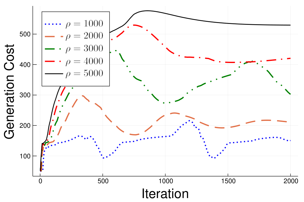
As we can see, the primal residual and generation costs exhibit oscillating patterns for $\rho\in\{1000,2000,3000,4000\}$, and do not converge even when ADMM has performed 2000 iterations. For $\rho=5000$, the primal residual converges to 0.0093, and the generation cost at termination is below the lower bound obtained from SOCP; these two facts indicate that ADMM indeed converges to an infeasible solution.

Such failures of ADMM to obtain feasible solutions result from the tension between the Assumptions (b) and (c) introduced in Section II-B. To be more specific, it is straightforward to verify that $\mathrm{Im}(B)\subset\mathrm{Im}(A)$: given a global copy $\bar{x}_{j}$, every local agent $l\in N(j)\cup R(j)$ can always keep the same value $x^{l}_{j}=\bar{x}_{j}$ so that the constraint $Ax+B\bar{x}=0$ is satisfied. Therefore, to satisfy Assumption (c), $A$ need to be the last block and $B$ is the first block in ADMM. But since each agent’s problem must consider local OPF constraints, which means $\mathcal{X}$ must be a nonconvex set. This violates the requirement that the problem of the last block must be unconstrained in Assumption (b). Therefore, Assumptions (b) and (c) cannot be satisfied simultaneously. As a result, if we directly apply ADMM to the ACOPF problem, ADMM may fail to converge. Admittedly, we observe convergence when a even larger penalty $\rho$ is used; however, we want to emphasize that despite the numerical success with adaptive parameter tuning [13], the traditional ADMM framework has no guarantee of convergence and could fail for nonconvex distributed OPF.

In this section we give a full description of the two-level algorithm applied to the OPF problem. The key idea is to dualize and penalize the constraint $z=0$ in (9), and apply three-block ADMM to solve the augmented Lagrangian relaxation (ALR):

with some dual variable $\lambda^{k}$ and penalty $\beta^{k}$, to an approximate stationary solution in the following sense.

Then at termination of ADMM, we update $\lambda^{k+1}$ and $\beta^{k+1}$ as in the classic ALM framework in order to drive $z$ to 0. To summarize, the proposed algorithm consists of two levels: in the inner level (indexed by $t$), we apply ADMM to solve the ALR problem (15); in the outer level (indexed by $k$), we update the dual information $(\lambda^{k+1},\beta^{k+1})$ using the solution $(x^{k},\bar{x}^{k},z^{k})$ returned by ADMM, which falls into the category of ALM, and then restart the next inner level. See Algorithm 1 for a detailed description.

The inner level is presented in line 4-11 of Algorithm 1, where we apply ADMM to solve ALR (15). To facilitate understanding, define the augmented Lagrangian function associated with (15) as

where $(\lambda^{k},\beta^{k})$ are considered as parameters. From a centralized point of view, equations (5)-(18) are the sequential minimization of $L_{\rho}$ with respect to $x\in\mathcal{X}$, $\bar{x}\in\bar{\mathcal{X}}$, and $z$, respectively, which, together with the update of dual variable $y$ in (19), constitute a single ADMM iteration. Next we describe ADMM from a local point of view. All agents simultaneously solve lower-dimensional nonconvex subproblems (5) by some nonlinear optimization solver. Then each agent $r\in[R]$ sends the current local estimate of voltage $(x^{r}_{j})^{t+1}$ to $R(j)$ for all neighboring buses $j\in\delta(\mathcal{R}_{r})$. For each bus $j$ connected to a tie-line, we let agent $R(j)$ collect estimates $\{(x^{l}_{j})^{t+1}\}_{l\in N(j)}$ and update global copy $(\bar{x}_{j})^{t+1}$, though in practice any agents from $N(j)$ can be assigned for this task. Notice that the global copy update (17) involves a projection evaluation, which in general does not admit a closed-form solution; however, if (10) is used for $\bar{\mathcal{X}}$, then $\bar{x}^{t+1}_{j}$ is exactly the component-wise projection of the argument in (17) onto the box $\bar{\mathcal{X}}_{j}$. After agent $R(j)$ broadcasts $(\bar{x}_{j})^{t+1}$ to agents from $N(j)$, all agents are then able to update the slack variable and dual variables as in (18) and (19).

When the inner-level iterates satisfy certain stopping criteria, all agents will update the outer-level dual variable $\lambda^{k+1}$ and penalty $\beta^{k+1}$, as in line 13 of Algorithm 1, which we will elaborate in the next section.

We consider two different rules for updating $(\lambda^{k+1},\beta^{k+1})$. Let $c>1$, $\theta\in[0,1)$, and $\{\eta_{k}\}_{k}$ be a nonnegative sequence convergent to 0:

and

Proof of Theorem 1 is provided in Appendix. We note that in part 3 of Theorem 1, we make the assumption that the dual variable $\{y^{k_{r}}\}_{r}$ has a limit point. This is a standard sequentially bounded constraint qualification (SBQC) [30].

References

- [1] D. Bienstock and A. Verma, “Strong NP-hardness of AC power flows feasibility,” arXiv preprint arXiv:1512.07315, 2015.
- [2] K. Lehmann, A. Grastien, and P. Van Hentenryck, “AC-feasibility on tree networks is NP-hard,” IEEE Transactions on Power Systems, vol. 31, no. 1, pp. 798–801, 2016.
- [3] R. A. Jabr, A. H. Coonick, and B. J. Cory, “A primal-dual interior point method for optimal power flow dispatching,” IEEE Transactions on Power Systems, vol. 17, no. 3, pp. 654–662, 2002.
- [4] R. D. Zimmerman, C. E. Murillo-Sánchez, R. J. Thomas et al., “Matpower: Steady-state operations, planning, and analysis tools for power systems research and education,” IEEE Transactions on power systems, vol. 26, no. 1, pp. 12–19, 2011.
- [5] X. Bai, H. Wei, K. Fujisawa, and Y. Wang, “Semidefinite programming for optimal power flow problems,” International Journal of Electrical Power & Energy Systems, vol. 30, no. 6-7, pp. 383–392, 2008.
- [6] J. Lavaei, D. Tse, and B. Zhang, “Geometry of power flows and optimization in distribution networks,” IEEE Transactions on Power Systems, vol. 29, no. 2, pp. 572–583, 2014.
- [7] R. A. Jabr, “Radial distribution load flow using conic programming,” IEEE transactions on power systems, vol. 21, no. 3, pp. 1458–1459, 2006.
- [8] B. Kocuk, S. S. Dey, and X. A. Sun, “Strong SOCP relaxations for the optimal power flow problem,” Operations Research, vol. 64, no. 6, pp. 1177–1196, 2016.
- [9] A. X. Sun, D. T. Phan, and S. Ghosh, “Fully decentralized AC optimal power flow algorithms,” in Power and Energy Society General Meeting (PES), 2013 IEEE. IEEE, 2013, pp. 1–5.
- [10] T. Erseghe, “Distributed optimal power flow using ADMM,” IEEE Transactions on Power Systems, vol. 29, no. 5, pp. 2370–2380, 2014.
- [11] ——, “A distributed approach to the OPF problem,” EURASIP Journal on Advances in Signal Processing, vol. 2015, no. 1, p. 45, 2015.
- [12] M. J. Feizollahi, S. Ahmed, and A. Sun, “Exact augmented Lagrangian duality for mixed integer linear programming,” Mathematical Programming, vol. 161, no. 1-2, pp. 365–387, 2017.
- [13] S. Mhanna, G. Verbic, and A. C. Chapman, “Adaptive ADMM for distributed AC optimal power flow,” IEEE Transactions on Power Systems, vol. 34, no. 3, pp. 2025–2035, May 2019. [Online]. Available: https://ieeexplore.ieee.org/document/8573893/
- [14] D. K. Molzahn, F. Dörfler, H. Sandberg, S. H. Low, S. Chakrabarti, R. Baldick, and J. Lavaei, “A survey of distributed optimization and control algorithms for electric power systems,” IEEE Transactions on Smart Grid, vol. 8, no. 6, pp. 2941–2962, 2017.
- [15] B. Houska, J. Frasch, and M. Diehl, “An augmented Lagrangian based algorithm for distributed nonconvex optimization,” SIAM Journal on Optimization, vol. 26, no. 2, pp. 1101–1127, 2016.
- [16] A. Engelmann, Y. Jiang, T. Mühlpfordt, B. Houska, and T. Faulwasser, “Toward distributed OPF using ALADIN,” IEEE Transactions on Power Systems, vol. 34, no. 1, pp. 584–594, 2018.
- [17] C. Coffrin, D. Gordon, and P. Scott, “Nesta, the nicta energy system test case archive,” arXiv preprint arXiv:1411.0359, 2014.
- [18] S. Babaeinejadsarookolaee, A. Birchfield, R. D. Christie, C. Coffrin, C. DeMarco, R. Diao, M. Ferris, S. Fliscounakis, S. Greene, R. Huang et al., “The power grid library for benchmarking AC optimal power flow algorithms,” arXiv preprint arXiv:1908.02788, 2019.
- [19] R. Glowinski and A. Marroco, “Sur l’approximation, par éléments finis d’ordre un, et la résolution, par pénalisation-dualité d’une classe de problèmes de dirichlet non linéaires,” Revue française d’automatique, informatique, recherche opérationnelle. Analyse numérique, vol. 9, no. R2, pp. 41–76, 1975.
- [20] D. Gabay and B. Mercier, “A dual algorithm for the solution of nonlinear variational problems via finite element approximation,” Computers & Mathematics with Applications, vol. 2, no. 1, pp. 17–40, 1976.
- [21] M. R. Hestenes, “Multiplier and gradient methods,” Journal of optimization theory and applications, vol. 4, no. 5, pp. 303–320, 1969.
- [22] M. J. Powell, A method for non-linear constraints in minimization problems. UKAEA, 1967.
- [23] F. Wang, Z. Xu, and H.-K. Xu, “Convergence of bregman alternating direction method with multipliers for nonconvex composite problems,” arXiv preprint arXiv:1410.8625, 2014.
- [24] Y. Wang, W. Yin, and J. Zeng, “Global convergence of ADMM in nonconvex nonsmooth optimization,” Journal of Scientific Computing, pp. 1–35, 2015.
- [25] B. Jiang, T. Lin, S. Ma, and S. Zhang, “Structured nonconvex and nonsmooth optimization: algorithms and iteration complexity analysis,” Computational Optimization and Applications, vol. 72, no. 1, pp. 115–157, 2019.
- [26] K. Sun and X. A. Sun, “A two-level distributed algorithm for general constrained non-convex optimization with global convergence,” arXiv preprint arXiv:1902.07654, 2019.
- [27] B. H. Kim and R. Baldick, “Coarse-grained distributed optimal power flow,” IEEE Transactions on Power Systems, vol. 12, no. 2, pp. 932–939, 1997.
- [28] R. T. Rockafellar and R. J.-B. Wets, Variational analysis. Springer Science & Business Media, 2009, vol. 317.
- [29] A. Wächter and L. T. Biegler, “On the implementation of an interior-point filter line-search algorithm for large-scale nonlinear programming,” Mathematical programming, vol. 106, no. 1, pp. 25–57, 2006.
- [30] Z.-Q. Luo, J.-S. Pang, D. Ralph, and S.-Q. Wu, “Exact penalization and stationarity conditions of mathematical programs with equilibrium constraints,” Mathematical Programming, vol. 75, no. 1, pp. 19–76, 1996.
- [31] I. Dunning, J. Huchette, and M. Lubin, “JuMP: A modeling language for mathematical optimization,” SIAM Review, vol. 59, no. 2, pp. 295–320, 2017.
- [32] G. Karypis and V. Kumar, “Multilevel k-way partitioning scheme for irregular graphs,” Journal of Parallel and Distributed computing, vol. 48, no. 1, pp. 96–129, 1998.
Appendix
VI-A Proof of Theorem 1
Proof.
The claims under condition (21) are proved in Theorem 1-2 of [26]. We shall prove the claims under condition (22).
- 1.
The first claim follows from the compactness of ’s and and the fact that .
- 2.
First we assume the sequence stays finite. Then there exists such that for all , which follows . Next assume , and assume without loss of generality that . If the first case in (22) is executed infinitely many times, we have ; otherwise we must have stays constant for all sufficiently large . Define . If has a bounded subsequence, then we have as converges to infinity. In all previous cases, we have , and thus . In the last case we have , stays bounded, and . By the definition of , we can see . At termination of ADMM, we have
(25a) (25b) (25c) where . By the closeness of normal cone, dividing vectors in (25a)-(25b) by , and then taking limit, we have and , which imply is stationary for (23).
- 3.
Using the same case analysis as in part 2), we can see (along the subsequence converging to ). Thus taking limit on (26) completes the proof.
∎
VI-B Proof of Theorem 2
We use to denote an upper bound of the number of inner iterations of the -th ADMM, which produces an -stationary solution point of (15) (see Definition 2) . By Lemma 3 of [26], upon termination of ADMM, we can find and corresponding such that