Path homology and temporal networks

Path homology of digraphs (briefly recalled in §2) was introduced in [7] and concurrent papers [8, 9, 10, 11, 12, 13], and it is increasingly being studied by practitioners of applied topology [1, 2, 4, 16, 19]. However, progress in empirical applications of path homology to digraph-structured data in general, especially large and/or complex digraphs, is obstructed by the difficulty of relating the algebraic information in homology to the combinatorial structure of the underlying digraph.

To help remedy this, in §3 we present an algorithm and implementation for computing path homology in arbitrary dimension with capabilities for symbolic output. We then use this algorithm in §4 to compute the path homologies of digraphs from the following families: (1) all digraphs on $\leq 4$ vertices, (2) all directed acyclic graphs on $\leq 6$ vertices, (3) all undirected graphs on $\leq 6$ vertices, (4) Erdős-Rényi random graphs, and (5) a family of graphs conjectured to exhibit torsion. These examples build intuition and provide digraph constructions with surprising path homologies.

Finally, we use this algorithm in §5 to compute path homologies of digraphs obtained from three temporal networks, identifying salient motifs of the sort found in §4 and relating them to the broader network behavior, before making concluding remarks in §6.

We outline path homology as treated in [7, 1]. For additional background on topology, including the theory of simplicial homology that shares many similarities with path homology, see [6, 14].

For a loopless digraph $D=(V,A)$, the set $\mathcal{A}_{p}(D)$ of allowed $p$-paths is

By convention, we take $\mathcal{A}_{0}:=V$, $V^{0}\equiv\mathcal{A}_{-1}:=\{0\}$ and $V^{-1}\equiv\mathcal{A}_{-2}:=\varnothing$. For a field $\mathbb{F}$ ¹¹ 1 Path homology can also be defined over rings such as $\mathbb{Z}$ without any modifications besides a change of notation. This definition gives additional power: M. Yutin has exhibited digraphs on as few as six vertices that have torsion: see Fig. 5. and a finite set $X$, let $\mathbb{F}^{X}\cong\mathbb{F}^{|X|}$ be the free $\mathbb{F}$-vector space on $X$, taking $\mathbb{F}^{\varnothing}:=\{0\}$. The non-regular boundary operator $\partial_{[p]}:\mathbb{F}^{V^{p+1}}\rightarrow\mathbb{F}^{V^{p}}$ is the linear map acting on the standard basis as

where $\nabla_{j}(v_{0},\dots,v_{p})$ notation means that $v_{j}$ is dropped from the tuple. A few lines of algebra suffice to confirm that $\partial_{[p-1]}\circ\partial_{[p]}\equiv 0$, so $(\mathbb{F}^{V^{p+1}},\partial_{[p]})$ is a chain complex, i.e., $\partial_{p-1}\circ\partial_{p}\equiv 0$, as indicated in Fig. 1.

This is important because any chain complex $(C_{p},\partial_{p})$ gives rise to an invariant called homology which behaves nicely with respect to maps on the chain complex induced by an underlying transformation of a common structure (here, a digraph). Writing $Z_{p}:=\text{ker }\partial_{p}$ and $B_{p}:=\text{im }\partial_{p+1}$, the dimension $p$ homology of the chain complex $(C_{p},\partial_{p})$ is the quotient

This is a finitely generated abelian group, thus of the form $\mathbb{Z}^{\beta_{p}}\oplus T_{p}$, where the torsion $T_{p}$ is a finite abelian group. Over a field, the $C_{p}$ are vector spaces and the torsion vanishes, in which case the Betti numbers $\beta_{p}:=\text{dim }H_{p}=\text{dim }Z_{p}-\text{dim }B_{p}$ fully capture the homology up to isomorphism.

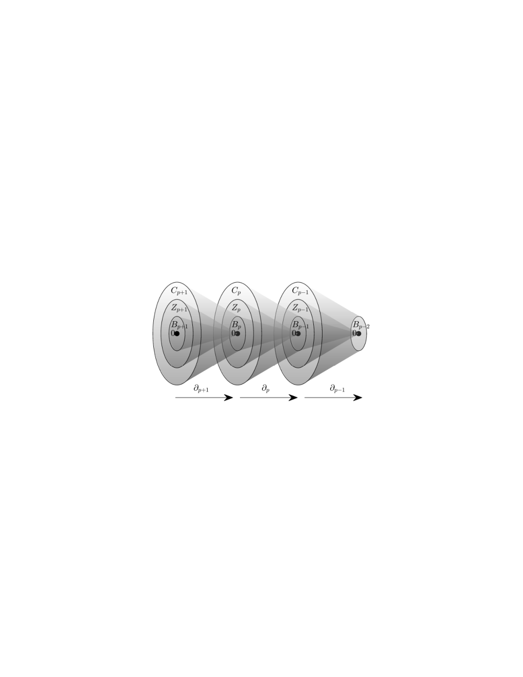
Path homology comes from a chain complex derived from $(\mathbb{F}^{V^{p+1}},\partial_{[p]})$. Set

$\Omega_{-1}:=\mathbb{F}^{\{0\}}\cong\mathbb{F}$, and $\Omega_{-2}:=\mathbb{F}^{\varnothing}=\{0\}$. We have that $\partial_{[p]}\Omega_{p}\subseteq\mathbb{F}^{\mathcal{A}_{p-1}}$, so $\partial_{[p-1]}\partial_{[p]}\Omega_{p}=0\in\mathbb{F}^{\mathcal{A}_{p-2}}$ and $\partial_{[p]}\Omega_{p}\subseteq\Omega_{p-1}$. The (non-regular) path complex of $D$ is accordingly defined as the chain complex $(\Omega_{p},\partial_{p})$, where $\partial_{p}:=\partial_{[p]}|_{\Omega_{p}}$. ²² 2 The implied regular path complex prevents a directed 2-cycle from having nontrivial 1-homology. While [7] advocates regular path homology, in our view non-regular path homology is simpler, richer, and more likely useful in applications. Our rationale amounts to the convention that a directed 2-cycle should count as a “hole.” The homology of this path complex is the (non-regular) path homology of $D$.

As a basic example illustrating the mechanics of path homology, consider the digraphs $D_{1}$ and $D_{2}$ in Figure 2. $\mathcal{A}_{1}(D_{1})$ and $\mathcal{A}_{1}(D_{2})$ are given by the digraph arcs, $\mathcal{A}_{2}(D_{2})=\varnothing$, and $\mathcal{A}_{2}(D_{2})=\{(w,x,z),(w,y,z)\}$. Now $\partial_{[2]}e_{(w,x,z)}=e_{(x,z)}-e_{(w,z)}+e_{(w,x)}\not\in\mathbb{F}^{\mathcal{A}_{1}(D_{2})}$ and $\partial_{[2]}e_{(w,y,z)}=e_{(y,z)}-e_{(w,z)}+e_{(w,z)}\not\in\mathbb{F}^{\mathcal{A}_{1}(D_{2})}$ (because the arc $w\rightarrow z$ is missing), so

Therefore the dimensions of the path homology vector spaces–i.e., the Betti numbers–are different: $\beta_{1}(D_{1})=1$ and $\beta_{1}(D_{2})=0$.

For convenience, we replace the path complex $(\Omega_{p},\partial_{p})$ with its reduction

which (using an obvious notational device and assuming the original complex is nondegenerate) has the minor effect $\tilde{H}_{0}\oplus\mathbb{F}\cong H_{0}$, while $\tilde{H}_{p}\cong H_{p}$ for $p>0$. Similarly, $\tilde{\beta}_{p}=\beta_{p}-\delta_{p0}$, where $\delta_{jk}:=1$ iff $j=k$ and $\delta_{jk}:=0$ otherwise.

Although an algorithm to compute non-regular path homology is fairly obvious, our implementation [28] is apparently among the first for dimension $>1$. Though [23, 24] are considerably older, we were unaware of these for some time and could not find any published work drawing on them, so we outline our approach here.

First, to reduce computation, we remove all nonbranching limbs (i.e. chains of vertices of total degree $2$ terminating in leaves of degree $1$), since these do not affect homology (Theorem 5.1 of [7]). Similarly (see Prop. 3.25 of [7]), we break the graph into weakly connected components and compute homology componentwise. For each component $D$, we extend an order on vertices $V(D)\equiv[n]$ to the lexicographical ordering on paths. We inductively construct $\mathcal{A}_{p}(D)$ for $0\leq p\leq p_{\max}$ as follows: $\mathcal{A}_{0}(D)=V(D)$, and $\mathcal{A}_{p}(D)$ is constructed by appending to every path in $\mathcal{A}_{p-1}(D)$ every vertex that has an arc from the path’s terminal vertex. The paths are constructed in lexicographical order for each $p$.

From here, we compute the indices (using a radix-$n$ expansion) that specify the inclusion $\mathcal{A}_{p}\hookrightarrow V^{p+1}$ under lexicographical ordering. We then construct the matrix representation $\partial_{[p,\mathcal{A}]}$ of the restriction of $\partial_{[p]}$ to $\mathbb{F}^{\mathcal{A}_{p}}$ using the standard basis. Let $\nabla_{[p,\mathcal{A}]}$ be the projection of $\partial_{[p,\mathcal{A}]}$ onto $\mathbb{F}^{V^{p}\backslash\mathcal{A}_{p-1}}$ (i.e., the matrix obtained by removing rows of $\partial_{[p,\mathcal{A}]}$ that correspond to elements of $\mathcal{A}_{p-1}$), and $\Delta_{[p,\mathcal{A}]}$ be the projection onto $\mathbb{F}^{A_{p-1}}$. The kernel of $\nabla_{[p,\mathcal{A}]}$ is $\Omega_{p}$. In practice, we remove rows of $\nabla_{[p,\mathcal{A}]}$ that are identically zero before computing this kernel, which yields $\Omega_{p}$ much more efficiently.

With a matrix representation $\Omega_{[p,\mathcal{A}]}$ for the kernel above in hand, we compute the chain boundary operator $\partial_{p}=\Omega_{[p-1,\mathcal{A}]}^{-1}\Delta_{[p,\mathcal{A}]}\Omega_{[p,\mathcal{A}]}$ (i.e., the projection of $\partial_{[p,\mathcal{A}]}$ onto $\mathbb{F}^{\mathcal{A}_{p-1}}$, projected onto and restricted to the invariant space). We then compute the homology of this chain complex, e.g. we use the rank-nullity theorem and compute the matrix ranks to obtain Betti numbers, or we compute representatives for the homology groups (albeit somewhat lacking in geometric meaning) as the cokernels of $[\ker\partial_{p}]^{T}\partial_{p+1}$, or take the Smith normal form of the boundary matrices to find any torsion over $\mathbb{Z}$ (cf. Fig. 5). ³³ 3 Further optimizations are imaginable. We can pre-process the graph more, in accord with Theorem 5.7 of [7], and deal with the fallout in low dimensions. Instead of performing a singular value decomposition on rather large boundary matrices (en route to computing the rank), we can recursively build up the invariant spaces from lower dimensions — each sub-path of an invariant path is itself an invariant path (since we assume no loops). A simple algorithm for this latter approach might be to check every pair of paths in dimension $p$ against every vertex to see where we can append ‘triangles’ and ‘squares’ (terminology borrowed from [7]); while promising, this approach generates too many paths, and reducing it to a basis is computationally nontrivial. For low dimensions, we could also directly compute Betti numbers from the digraph itself (e.g. Proposition 3.24 of [7]).

We analyze three temporal networks [15, 20], more specifically directed contact networks as described in [3]: MathOverflow, an email network, and activity on a Facebook group: these illustrate how path homology can find high-order interactions that are respectively indicators of dilution, recurring motifs, and concentration within network behavior.

Although the computational requirements for path homology scale exponentially with dimension $p$, even the case $p=2$ can highlight salient network structure and behavior. By decomposing temporal networks into time windows, path homology can be successfully brought to bear in this regard, illuminating both motifs with nontrivial path homology as well as the temporal networks themselves.

The authors thank Michael Robinson for many helpful discussions. This material is based upon work partially supported by the Defense Advanced Research Projects Agency (DARPA) and the Air Force Research Laboratory (AFRL). Any opinions, findings and conclusions or recommendations expressed in this material are those of the author(s) and do not necessarily reflect the views of DARPA or AFRL.

References

- [1] Chowdhury, S. and Mémoli, F. “Persistent path homology of directed networks.” Symposium on Discrete Algorithms (2018).
- [2] Chowdhury, S. et al. “Path homologies of deep feedforward networks.” IEEE International Conference on Machine Learning and Applications (2019).
- [3] Cybenko, G. and Huntsman, S. “Analytics for directed contact networks.” Appl. Net. Sci. 4, 106 (2019).
- [4] Dey, T. K., Tianqi, L., and Wang, Y. “An efficient algorithm for -dimensional (persistent) path homology.” Symposium on Computational Geometry (2020).
- [5] Frieze, A. and Karoński, M. Introduction to Random Graphs. Cambridge (2016).
- [6] Ghrist, R. Elementary Applied Topology. Createspace (2014).
- [7] Grigor’yan, A. et al. “Homologies of path complexes and digraphs.” arXiv:1207.2834 (2012).
- [8] Grigor’yan, A., Muranov, Yu., and Yau, S.-T. “Graphs associated with simplicial complexes.” Homology Homotopy Appl. 16, 295 (2014).
- [9] Grigor’yan, A. et al. “Homotopy theory for digraphs.” Pure Appl. Math. Quart. 10, 619 (2014).
- [10] Grigor’yan, A. et al. “Cohomology of digraphs and (undirected) graphs.” Asian J. Math. 19, 887 (2015).
- [11] Grigor’yan, A., Muranov, Yu., and Yau, S.-T. “Homologies of graphs and Künneth formulas.” Comm. Anal. Geom. 25, 969 (2017).
- [12] Grigor’yan, A. et al. “On the path homology theory of digraphs and Eilenberg-Steenrod axioms.” Homology Homotopy Appl. 20, 179 (2018).
- [13] Grigor’yan, A. et al. “Path homology theory of multigraphs and quivers.” Forum Math. 30, 1319 (2018).
- [14] Hatcher, A. Algebraic Topology. Cambridge (2002).
- [15] Holme, P. “Modern temporal network theory: a colloquium.” Eur. Phys. J. B 88, 234 (2015).
- [16] Huntsman, S. “Generalizing cyclomatic complexity via path homology.” arXiv:2003.00944 (2020).
- [17] Kunegis, J. “The Koblenz network collection.” WOW (2013).
- [18] Lescovec, J. and Krevl, A. “SNAP datasets: Stanford large network dataset collection.” http://snap.stanford.edu/data (2014).
- [19] Lin, Y., et al. “Weighted path homology of weighted digraphs and persistence.” arXiv:1910.09891 (2019).
- [20] Masuda, N. and Lambiotte, R. A Guide to Temporal Networks. World Scientific (2016).
- [21] Milo, R. “Network motifs: simple building blocks of complex networks.”Science 298.5594, 824-827 (2002).
- [22] Montoya, L. V., Ma, A., and Mondragón, R. J. “Social achievement and centrality in MathOverflow.” Complex Networks (2013).
- [23] Shajii, A. R. https://github.com/arshajii/digraph-homology (2013).
- [24] Slawinski, M. https://github.com/gtownrocks/digraph_homology (2013).
- [25] Tausczik, Y. R., Kittur, A., and Kraut, R. E. “Collaborative problem solving: a study of MathOverflow.” CSCW (2014).
- [26] Viswanath, B. et al. “On the evolution of user interaction in Facebook.” WOSN (2009).
- [27] Yutin, M. Personal communication. (2019).
- [28]
Yutin, M.
https://github.com/SteveHuntsmanBAESystems/PerformantPathHomology (2020).