Quantum Lifshitz points and fluctuation-induced first-order phase transitions in imbalanced Fermi mixtures
Abstract
We perform a detailed analysis of the phase transition between the uniform superfluid and normal phases in spin- and mass-imbalanced Fermi mixtures. At mean-field level we demonstrate that at temperature the gradient term in the effective action can be tuned to zero for experimentally relevant sets of parameters, thus providing an avenue to realize a quantum Lifshitz point. We subsequently analyze damping processes affecting the order-parameter field across the phase transition. We show that, in the low energy limit, Landau damping occurs only in the symmetry-broken phase and affects exclusively the longitudinal component of the order-parameter field. It is however unavoidably present in the immediate vicinity of the phase transition at temperature . We subsequently perform a renormalization-group analysis of the system in a situation, where, at mean-field level, the quantum phase transition is second order (and not multicritical). We find that, at sufficiently low, including the Landau damping term in a form derived from the microscopic action destabilizes the renormalization group flow towards the Wilson-Fisher fixed point. This signals a possible tendency to drive the transition weakly first-order by the coupling between the order-parameter fluctuations and fermionic excitations effectively captured by the Landau damping contribution to the order-parameter action.
I Introduction
Ultracold Fermi gases have been a topic of growing interest over the last years.Gurarie and Radzihovsky 2007; Bloch et al. 2008; Giorgini et al. 2008; Gubbels and Stoof 2013; Gross and Bloch 2017; Strinati et al. 2018; Cooper et al. 2019 This is related to the rich phenomenology involving the interplay of quantum statistics and interaction effects, including aspects hardly reachable or controllable in traditional electronic systems. A standard example is the BEC-BCS crossover,Zwerger 2012; Randeria and Taylor 2014 experimentally realized by resonantly controlled -wave interaction strength between particles in different pseudospin states. In Fermi mixtures, the possibility of tuning the populationZwierlein et al. 2006; Partridge et al. 2006; Ketterle et al. 2009 and mass imbalanceWille et al. 2008; Tiecke et al. 2010; Trenkwalder et al. 2011; Jag et al. 2014; Ravensbergen et al. 2018; Ravensbergen et al. 2020; Neri et al. 2020; Hara et al. 2011 allows for studying unconventional pairing phenomena leading to unusual superfluid phases such as the breached pair (Sarma-Liu-Wilczek) superfluidsSarma 1963; Liu and Wilczek 2003 or the Fulde-Ferrell-Larkin-Ovchinnikov (FFLO) phases.Fulde and Ferrell 1964; Larkin and Ovchinnikov 1965
Of substantial interest are quantum phase transitions between the superfluid and the normal, Fermi-liquid-like phases in imbalanced systems.Iskin and Sá de Melo 2007; Parish et al. 2007a; Radzihovsky and Sheehy 2010; Klimin et al. 2012; Gubbels and Stoof 2013; Strack and Jakubczyk 2014; Roscher et al. 2015; Wang et al. 2017 Increasing the composition- (and/or mass-) imbalance mismatches the Fermi surfaces and suppresses pairing. The population and/or mass imbalance therefore play the role of realistically controllable parameters to tune the system across the phase transition both at temperature and .
An interesting, and, thus far, not fully explored aspect of the phase diagram of Fermi mixtures concerns multicritical phenomena. It is well recognized that, in a typical situation, the phase transition between the uniform superfluid and normal phases is first-order for sufficiently low, and necessarily becomes continuous for higher, above a tricritical temperature .Parish et al. 2007b; Lamacraft and Marchetti 2008; Chevy and Mora 2010 It has, however, recently been shownZdybel and Jakubczyk 2018 that (in dimensionality ) can actually be suppressed to zero for sufficiently large mass imbalance. In this situation, the phase diagram exhibits a quantum critical point (QCP). As was indicated by mean-field studies, there is however another, quite distinct multicritical phenomenon present at , related to the so-called Lifshitz point,Gubbels et al. 2009; Baarsma et al. 2010 where two ordered phases (uniform and nonuniform superfluids) coexist with the normal phase. The universal critical singularities at the classical () Lifshitz pointDiehl 2002; Diehl et al. 2003; Zappalà 2018 are completely different from those controlling the critical or tricritical point. Notably, while the upper critical dimension for the tricritical transition is 3, it is way higher (at least 9/2) for the Lifshitz transition,Diehl 2002; Essafi, K. et al. 2012; Zappalà 2017 making the conventional approaches to critical phenomena in spatial dimensionality based on the -expansion () problematic.Essafi, K. et al. 2012 The presence of a Lifshitz point additionally leads to rich and interesting crossover phenomena.Diehl 2002
Phase transitions at and are driven by thermal and quantum fluctuations respectively. The natural question concerning the physics of imbalanced Fermi gases is whether the Lifshitz point may be suppressed to zero temperature and arise as a result of purely quantum fluctuations. In this paper we give a positive answer to this question, deriving an analytical mean-field criterion for the occurrence of such a quantum Lifshitz point and providing a proposal for its potential experimental realization.
The second problem addressed in the present paper concerns the nature of the quantum phase transition between the normal and uniform superfluid phases in a situation when the transition is continuous (and not multicritical) at mean-field level. The general approach to quantum criticality in Fermi systems, based on an effective bosonic mode is recognized as the Hertz-Millis theory.Hertz 1976; Millis 1993 Within this approach, the interaction between the collective order-parameter mode and soft fermionic excitations across the Fermi surface is captured by the so-called Landau-damping term, appearing in the inverse propagator of the order-parameter mode. The presence (or absence) of Landau damping, as well as its precise form has profound impact on the quantum critical behavior, in particular it determines the value of the dynamical critical exponent , which in turn influences many thermodynamic and transport properties. As was shown in Ref. Zdybel and Jakubczyk 2019, Landau damping is always present in the ordered phase in the vicinity of the imbalance-driven superfluid quantum phase transition. We here supplement and extend the analysis of Ref. Zdybel and Jakubczyk 2019 by further elucidating the nature of Landau damping in the superfluid phase. In particular, we demonstrate that it affects exclusively the longitudinal component of the order-parameter field. By considering the normal phase, we show in turn that Landau damping is absent therein. This constitutes a situation different as compared to that studied for magnetic quantum critical points and requires a renormalization-group (RG) treatment formulated in the ordered phase. We address this problem within the framework of non-perturbative RG. Our results, based on a very simple truncation of a functional RG flow equation, recover the expected behavior of the system in absence of Landau damping. However, for temperatures low enough, the presence of Landau damping in the form derived from the microscopic model turns out to destabilize the expected flow towards the Wilson-Fisher fixed point, so that the asymptotic scaling regime is not reached. This behavior may indicate a fluctuation-driven first-order transition induced by Landau damping and would constitute a mechanism for fluctuation driven first order phase transitions entirely different as compared to the one well-studied e.g. for the ferromagnetic quantum phase transition.Belitz et al. 2005a
The outline of the present paper is as follows: In Sec. II, focusing on the symmetry-broken phase, we summarize the structure of the effective order-parameter action employed in our study of the superfluid phase transition. Sec. III contains an analysis of the pair fluctuation propagator in the normal phase, in particular the properties of the gradient expansion (including both analytical and non-analytical contributions). This leads to insights concerning order-parameter excitations as well as the dominant instabilities towards the uniform or non-uniform ordered phases. We derive a criterion for the occurrence of a quantum Lifshitz point and discuss its phenomenological implications. We subsequently discuss the nature of the (nonlocal) terms related to Landau damping and demonstrate their absence in the normal phase in the low-energy limit. In Sec. IV we present a study of order parameter fluctuation effects focusing on a situation, where the quantum phase transition is second-order (and not multicritical) at mean-field level. We emphasize the necessity to formulate the RG in the symmetry-broken phase.Jakubczyk et al. 2008 We discuss the effect of destabilizing the RG flow towards the Wilson-Fisher fixed point at temperatures () sufficiently low caused by the Landau damping. We summarize the paper in Sec. V.
II Effective action
We consider a two-component fermionic mixture of particles of masses and chemical potentials [], where an attractive interspecies contact interaction triggers -wave pairing. The system is described by the microscopic action
| (1) |
and the grand-canonical partition function reads
| (2) |
Here are Grassmann fields, , denotes the dispersion relation and collects the (fermionic) Matsubara frequency and momentum . Throughout the paper we put and use the shorthand notation .
The effective action for the order-parameter field can be derived using a standard procedure described in detail in Ref. Iskin and Sá de Melo 2007. We decouple the interaction term in Eq. (1) into the Cooper channel via the Hubbard-Stratonovich transformation.Altland and Simons 2010 This introduces the -wave pairing field conjugate to the fermionic bilinear . Subsequently we integrate out the Grassmann fields , which leads to a purely bosonic description of the system. We obtain the following expression
| (3) |
where , and is the bosonic pairing field split into the uniform contribution and fluctuation (notice that . The quantity encompasses the (bosonic) Matsubara frequency and momentum . All the momentum expansions will now be performed around which restricts the results below to uniform phases. Nonuniform ordering tendencies are discussed in Sec. III.
The term may be written as
| (4) |
where collects the imaginary time and position vector, while . The effective potential takes the formZdybel and Jakubczyk 2018
| (5) |
where and
| (6) |
is the excitation energy of fermionic quasiparticles. The global minimum of determines the mean-field grand-canonical potential per unit volume.
Of our major present interest is the inverse Gaussian pair fluctuation propagator matrix in Eq. (3), encoding the dynamical characteristics of the collective excitations in the system. Its properties in the superfluid phase were recently addressed in Ref. Zdybel and Jakubczyk 2019, leading inter alia to the conclusion that Landau damping of the Anderson-Bogolyubov mode is unavoidable close to the quantum phase transition approaching from the superfluid phase. Damping brings about modification of the dynamics of the system, which is manifested by terms in a gradient expansion of matrix elements of the inverse propagator . Denoting , we obtainZdybel and Jakubczyk 2019
| (7) |
| (8) |
where we parametrize the action in such a way that terms are contained in the local potential term . The quantities may be related to the parameters of the microscopic fermionic action , while . It is noteworthy that contributions related to the damping of collective modes are proportional to . In the superfluid phase, the quasiparticles are a superposition of particle-like and hole-like excitations.Pieri et al. 2004; Strinati et al. 2018 As a consequence, in the evaluation of the matrix elements of , both particle-particle and particle-hole bubble diagrams may give a contribution.Pieri et al. 2004 Pair fluctuations couple with fermionic particle-hole excitations across the Fermi level, which gives rise to the Landau damping.Kurkjian and Tempere 2017; Klimin et al. 2019 However, once we move to the normal phase (), the particle-hole continuum vanishes, and damping terms disappear.Zdybel and Jakubczyk 2019 This manifests itself by the proportionality of the damping terms to . This feature makes the nature of the phase transition in imbalanced Fermi mixtures distinct from those studied in the context of magnetic phase transitions (see e.g. Refs. Nagaosa 1999; Continentino 2017; Belitz et al. 2005a; Löhneysen et al. 2007).
We now decompose using the cartesian representation
| (9) |
where and are bosonic fields describing longitudinal and transverse fluctuations of the pairing field, respectively. The uniform contribution is chosen real. We have and since and are real fields. Inserting the decomposition of Eq. (9) into Eq. (3) and parametrizing the effective potential via a quartic form
| (10) |
leads to
| (11) |
where the quadratic terms are obtained as
| (12) |
| (13) |
| (14) |
Here is a mass of the -field, , , and .
For the obtained action is reminiscent of the one studied for interacting bosons (see e.g. Pistolesi et al. 2004; Obert et al. 2013). As expected, the transverse -mode is massless. We observe that the Landau damping term occurs only in the longitudinal mode. We also note that its presence was not taken into account in previous studies of fluctuation effects in imbalanced Fermi systems (e.g. Strack and Jakubczyk 2014; Boettcher et al. 2015; Zdybel and Jakubczyk 2018).
III Pair fluctuation propagator in the normal phase
We now set out to analyze the structure of the pair fluctuation propagator in the normal phase. We focus on dimensionality and the situation, where (at mean-field level) the phase transition is continuous down to . As was shown in Ref. Zdybel and Jakubczyk 2018, this is achievable for the mass ratio . Note that (at mean field level) this is very different from the case , where the corresponding quantum phase transition is always discontinuous, but may be driven second-order by order-parameter fluctuation effects.Strack and Jakubczyk 2014 We treat the ”Zeeman” field as the control parameter tuning the system towards the phase transition. The system remains disordered for , where may be expressed via the microscopic model parameters.Zdybel and Jakubczyk 2018 The occurrence of an instability towards a non-uniform (FFLO) superfluid manifests itself by a negative gradient coefficient (see below), which is of our particular interest in Sec. IIIA. We present a schematic mean-field phase diagram in Fig. 1. Note that the typical profile of the phase boundary shows reentrant behavior for large enough.Zdybel and Jakubczyk 2018; Parish et al. 2007b

We employ the Noziriès-Schmitt-Rink methodNozières and Schmitt-Rink 1985 focusing on zero temperature and the vicinity of the phase transition.Liu and Hu 2006 We compute the inverse pair fluctuation propagator by evaluating the particle-particle bubble diagramStrinati et al. 2018
| (15) |
where is the reduced mass, and . In the above expression, we regularized the integral using the Lipmann-Schwinger equationStoof et al. 2009
| (16) |
where is the fermionic -wave scattering length, and the integrals are cutoff at momentum . The procedure eliminates ultraviolet divergencies in the limit and while keeping constant.Strinati et al. 2018
We perform analytical continuation () of Eq. (15), and separate the obtained retarded counterpart of into real and imaginary parts using the Sokhotski formula where is the Cauchy principal value. As a result, we find
| (17) |
and
| (18) |
The present treatment is in a way parallel to that employed in the context of the random phase approximation for plasmons in the homogeneous electron gas,Jishi 2013 where however the bosonic propagator contains the particle-hole bubble diagram instead of the particle-particle one.
III.1 Gradient expansion and the quantum Lifshitz point
Focusing on we perform the low-frequency and low-momentum expansion of . We take into account terms up to second order in and . This leads to
| (19) |
The gradient coefficients as well as can be determined analytically in the limit , where . The constant contribution corresponds to the Landau coefficient of and is given byZdybel and Jakubczyk 2018
| (20) |
where is the ”average” Fermi momentum, denotes the ””-particle () Fermi momentum and is the ”average” chemical potential. Within mean-field theory in the normal phase, and . The gradient coefficients are given by
| (21) |
| (22) |
and
| (23) |
The sign of determines whether, for vanishing , the system tends to condense in the uniform (BCS-type) or non-uniform (FFLO) ground state. We are now interested in a situation, where both and are zero, which provides a criterion for the occurrence of a (quantum) Lifshitz point. We introduce as a value of defined by the condition and analyze the situation, where . It is worth noting that do not depend on the scattering length . One may therefore tune the system to , and independently vary to adjust towards . In Fig. 3. we plot for the experimentally realized mixture of 161Dy and 40K atoms,Ravensbergen et al. 2018; Ravensbergen et al. 2020 which is characterized by and .
We adapt the value of (see Eq. 20) to by manipulating the parameter [see Fig. 3]. The quantum Lifshitz point corresponds to in this situation. We also note that for the physically relevant range of parameters the coefficients and are positive, monotonously decreasing functions of .
An analogous reasoning may be carried out for other experimentally studied Fermi mixtures characterized by sufficiently large mass imbalance . Examples are the 6Li-40K mixtureWille et al. 2008; Tiecke et al. 2010; Trenkwalder et al. 2011; Jag et al. 2014 () as well as the 6Li-53Cr mixtureNeri et al. 2020 (). The quantum Lifshitz point is then obtained for and respectively (with in each case). In general, the value of is reduced upon increasing since a larger mass difference results in the occurrence of the FFLO pairing for smaller population asymmetry.
The occurrence of the quantum Lifshitz point has profound influence on the scaling behavior of the system for . The RG fixed point controlling the phase transition at may then be non-gaussian even for , unlike the typical situations recognized in electronic systems. Bringing the system to the proximity of the scenario discussed above should also yield complex and interesting crossover behavior. Resolution of the critical singular behavior at for the discussed Lifshitz transition is beyond the scope of the present paper, but certainly depends on the form of the damping term in the propagator (see the next sections), and, therefore will not fall into any of the classes discussed in the context of magnetic instabilities in electronic systems.Ramazashvili 1999; Continentino 2004 It may also be sensitive to the instability discussed in Sec. IV.
We finally point out, that, in a beyond-mean-field picture, the FFLO-type phases are suspectedRadzihovsky 2011; Jakubczyk 2017; Wang et al. 2018 to be marginally unstable to fluctuation effects in dimensionality at (but not at ). This would imply that, at least for infinite and homogeneous systems, the quantum Lifshitz point should always occur in the phase diagram if there is a phase transition between the FFLO-type and uniform superfluid phases at .
III.2 Landau damping
We now analyze the imaginary part of the retarded inverse propagator at . Whenever , the complex pole of develops, which leads to broadening of the peak corresponding to a collective mode in the spectral density function .Altland and Simons 2010; Jishi 2013 As a result, Landau damping emerges and the lifetime of collective excitations is finite. This issue was studied within the superfluid state,Kurkjian and Tempere 2017; Klimin et al. 2019; Zdybel and Jakubczyk 2019 but not in the normal phase.
We consider the limit in Eq. (18) and introduce . Angular integration leads to
| (24) | ||||
where . In the above expression we observe that may be nonzero only if . Thus, for values of ,Zdybel and Jakubczyk 2018 where the phase transition occurs, damping is absent for low energies in the normal phase.
The integrand in Eq. (24) is equal unity in the interval and zero otherwise. Only are physically relevant. These values are obtained as:
| (25) |
where and . The above expression is real when . As we find, iff , which divides the -plane into three distinct regions.

The first of them (reg. 1) is defined by . Here Landau damping is present and is given by
| (26) |
Analogously, the second regime (reg. 2) is obtained from the condition . In this situation damping is active as well, but the form of reads
| (27) |
where . The last regime (reg. 3) occurs whenever . Here and Landau damping is absent. The obtained results are schematically summarized in the diagram of Fig. 4.
The obtained picture has a transparent physical interpretation. In our reasoning we identified two conditions: (a) and (b) . Violation of any of them implies that . Recall that the quantum phase transition takes place between a fully-polarized gas and the superfluid phase. Thus, ””-particles are absent in the normal phase at , which is implied by for . We may reformulate the condition (a) as , which means that damping may occur only when the energy is high enough to introduce the ””-particle into the system. On the other hand, we may also restate the condition (b) as , where is the mass of a pair composed of ”” and ”” particles, and is its chemical potential. Therefore, damping may be active only when the excitation of a pair carrying momentum is achievable.
However, conditions (a) and (b) do not take into account the momentum conservation, which leads to further restrictions of areas in which . In particular, the step function in Eq. (24) inflicts values of and , which are consistent with possible directions of the momentum given by .
We note that is a non-positive function of and in both regions where Landau damping is active. This feature ensures that the spectral density function is non-negative for all values of and .
Notice, that at small damping occurs for , because .Zdybel and Jakubczyk 2018 Therefore, in the proximity of the quantum phase transition within the normal phase, the damping terms do not appear in the low-frequency and low-momentum expansion. As already emphasised, this situation is entirely different as compared to the symmetry-broken phase (see Sec. II).
In the following Sec. IV we analyze the impact of the Landau damping in the form discussed in Sec. II on the renormalization group flow in the vicinity of the quantum critical point.
IV Renormalization group flow
We now focus on the situation, where the phase transition between the normal and uniform superfluid phases is second order (and not multicritical). We examine fluctuation effects within the renormalization group framework. We connect to the Hertz-Millis theoryHertz 1976; Millis 1993 which originally was formulated with reference to the symmetric phase and addressed magnetic phase transitions in itinerant Fermi systems. An important insight of the Hertz-Millis theory is that the (second-order) quantum phase transition at belongs to the universality class of the appropriate -symmetric model in effective dimensionality , where the dynamical exponent takes the value for instabilities at ordering wavevector . The value of stems from Landau damping and the present situation is, from this perspective, not immediately obvious, since Landau damping is present only in the symmetry-broken phase and the coefficient of the term is proportional to and therefore vanishes at the critical point. We further note that the quantum critical point corresponds to a state, which is ordered at the level of the mean-field theory so that the Landau-damping term is present in the entire (critical) renormalization group flow and vanishes only for asymptotically low RG scales. The Hertz-Millis theory is, on the other hand, formulated in the symmetric phase. Below we employ a non-perturbative renormalization group framework applicable to both symmetric and symmetry-broken phasesJakubczyk et al. 2008 and capturing both the Gaussian and Wilson-Fisher fixed points. We show how the expected quantum-classical crossover at is accurately recovered by our approach in absence of Landau damping. We subsequently include the Landau damping term . Our results indicate that this leads to an obstruction of the RG flow towards the Wilson-Fisher fixed point occurring at intermediate RG scales and point towards a possible occurrence of a fluctuation-induced weakly first order phase transition driven by Landau damping of the longitudinal () mode. The mechanism of destabilizing the quantum critical point active here is entirely different from those studied beforeBelitz et al. 2005a; Löhneysen et al. 2007 e.g. for the ferromagnetic transitionsBelitz et al. 2005b or superconductors.Halperin et al. 1974; Li et al. 2009
We employ the one-particle-irreducible variant of nonperturbative renormalization theory, taking the Wetterich equationWetterich 1993
| (28) |
as the starting point. This framework is exceptionally convenient for resolution of crossover phenomena due to multiple fixed points governing the RG flow at distinct scales (see e.g. Refs. Strack and Jakubczyk 2009; Léonard and Delamotte 2015; Lammers et al. 2016; Debelhoir and Dupuis 2016; Rançon and Dupuis 2017; Chlebicki and Jakubczyk 2019). Eq. (28) describes the renormalization group flow of the effective action upon reducing the RG scale, implemented here as the momentum cutoff with and denoting the microscopic momentum scale. The quantity thus continuously connects the microscopic action and the thermodynamic free energy .
In the shorthand notation used in Eq. (28) the dot indicates differentiation with respect to the logarithmic scale , i.e. , the two-component real field is decomposed (compare Sec. II) into the longitudinal and transverse modes with chosen real, denotes the cutoff function added to the inverse propagator to regularize the low-momentum fluctuations. Finally, is the regularized propagator, obtained by taking the second field derivative of the regularized action in the direction. For a detailed exposition of the framework, we refer to Refs. Berges et al. 2002; Kopietz et al. 2010; Polonyi and Schwenk 2012; Dupuis et al. 2020. The approximation strategy taken below is an adaptation of the framework developed in previous studies of magnetic phase transitions in Fermi systems with Ising symmetryJakubczyk et al. 2008; Jakubczyk 2009; Jakubczyk et al. 2010 and conventional Hertz-Millis action. For the reason of highly anisotropic propagator obtained in the previous sections [Sec. II and III], we use two different cutoff functions for the distinct directions. We aim here at distilling the impact of the specific form of the Landau-damping term on the quantum-critical scaling, and, for the sake of simplicity, we will neglect the off-diagonal propagator. This term is absent for particle-hole symmetric systems and is supposed to scale to zero under RG flow in the entire symmetry-broken phase.Obert et al. 2013 In generality, it however influences some of the transport and thermodynamic properties, such as the condensate compressibility.Pistolesi et al. 2004
With this simplified picture in mind, proceeding along the standard track,Berges et al. 2002 we obtain the flow of the effective potential by evaluating the Wetterich equation [Eq. (28)] at a constant field configuration. This yields
| (29) |
where, within our parametrization, the inverse propagators are given by:
| (30) |
and
| (31) |
In what follows, we parametrize the flowing effective potential with the simple quartic form
| (32) |
In the present approximation, we also neglect the flow of the gradient coefficients (both in the space and time directions). This is equivalent to dropping the anomalous dimensions (which are anyway small for the three-dimensional systems studied here). In consequence, the RG flow is parametrized by a set of only two flowing couplings ( and ). In contexts concerning quantum criticality in itinerant Fermi systems (see. e.g. Ref. Jakubczyk et al. 2010) this simple approximation level captures the relevant aspects of physics in dimensionality . Note however, that it is quite insufficient in , where the flow of the -factors and the related anomalous dimensions play a prominent role.
We now extract the flow of from . Differentiating Eq. (29) we obtain
| (33) |
where we denoted The flow of the quartic interaction coupling is obtained by taking the second -derivative of Eq. (29) and evaluating at . This yields:
| (34) |
Note that since , putting leads to a massless -propagator [Eq. (31)]. The mass of the -propagator is on the other hand given by . As concerns the cutoff: in the following calculation we implement the direction-dependent Litim cutoffLitim 2001
| (35) |
where
| (36) |
and
| (37) |
With this convenient choice the integrals in the flow equations for and become effectively constrained to the regions of the space, where and are constant (i.e. -independent), which yields the momentum integrals straightforward. In what follows, we use the set of variables rescaled according to the canonical classical dimensions:
| (38) |
so that at the flow manifestly reaches the (Wilson-Fisher) fixed point if the initial condition for the flow is chosen at the critical manifold. The right-hand sides of the flow equations are split into the classical () and quantum () contributions, so that
| (39) |
| (40) |
We additionally separated the quantum contributions from the longitudinal () and transverse () fluctuations [compare Eq. (33) and (34)]. The Matsubara summations occurring in the quantum contributions must be carried our numerically. The explicit expressions for the flow equations are given in the appendix. The flow equations are written for arbitrary dimensionality , from now on we however restrict to . As already mentioned, the present approximation level is inadequate for the case since the anomalous dimensions are neglected. The critical singularity is controlled by the Gaussian fixed point at and by the classical Wilson-Fisher fixed point for .
IV.1 RG flow in absence of Landau damping
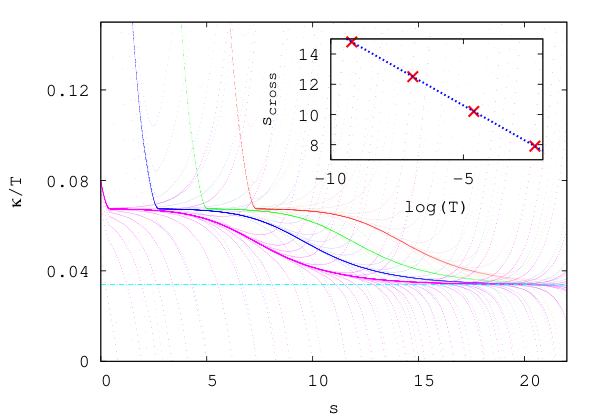
We now summarize the renormalization group flow neglecting the Landau damping of the longitudinal mode. This amounts to putting in and . The flow is initiated at with fixed temperature and given values of and deriving from the microscopic values. In the numerical solutions presented below we put . Integrating the flow towards large positive values of (corresponding to ) we find either reaching zero at a finite scale, indicating flow into the symmetric phase, or its divergence for large (corresponding to converging to a finite value), indicating the symmetry-broken state. By tuning the system towards the phase transition, we observe the flow of towards fixed-point values. The results for the flow of are exhibited in Fig. 5 for a sequence of temperatures approaching zero. The crossover scale, where the flow departs from the Gaussian fixed point (governing the critical singularity at ) and flows towards the Wilson-Fisher fixed point (controlling the critical singularity at ) diverges for according to [see Ref. (Millis 1993)]. A data fit gives in full accord with the expected behavior. The momentum range corresponds to the flow regime dominated by the quantum () contributions, while the range is dominated by the classical () contribution to the flow equations.
We now present the results obtained for the critical line by integrating the RG flow. The general expectationMillis 1993 yields (for low) the power-law behavior
| (41) |
Note that as given by this formula, depends exclusively on and and appears completely insensitive to the nature of the symmetry-broken phase. Exemplary results for the critical line, obtained by integrating the flow equations [Eq. (39), (40)] are presented in Fig. 6.
The obtained power law yields in full agreement with the expected behavior with (). Also observe, that the universal shape of the -line is incompatible with the reentrant behavior quite generically obtained at mean field level (see the illustrative Fig. 1, and e.g. Ref. Zdybel and Jakubczyk 2018).
The above calculation reproduces the anticipated picture of quantum criticality upon dropping the Landau damping term in the flow equations. We emphasize the role of the dynamical exponent, which governs both the -line and the quantum-classical crossover scale. It is now our aim to investigate how this picture becomes deformed if the Landau damping contribution to the -mode propagator (as found in the effective action analyzed in Sec. II and III) is included.
IV.2 RG flow in presence of Landau damping
We proceed by repeating the analysis of the previous subsection for nonzero Landau damping coupling . We solve the flow equations [Eq. (39-40)] following the procedure of tuning towards its critical value for a sequence of temperatures approaching zero. The quantum regime of the flow is now governed by the interplay of the distinct contributions (coming from the terms and ). The analysis of the flow of is depicted in Fig. 7 for a relatively small value of () and low temperature. The flow is superimposed with the corresponding situation obtained at the same (as well as the remaining parameters) for . The dichotomy procedure as described in the previous subsection leads to identification of the two phases present in the system as well as the phase boundary in the parameter space. The phase transition is however not accompanied by the convergence of the flow to the fixed point and the associated scale-invariance. This behavior may indicate a fluctuation-induced first-order transition originating from Landau damping.

The effect occurs only for temperatures sufficiently low, at higher we find a continuous transition as before. This would imply the presence of a tricritical point at a temperature in the phase diagram. We note that for the system shows behavior very similar to what we obtained for . The value of increased with and for the critical value of the control parameter is practically independent of , so that the -line in the plane is a vertical straight line. The obtained -line is plotted in Fig. 8 for a sequence of values of . Clearly visible is the deviation from the scaling behavior with at low .
Below the lowest-lying point in each of the plotted curves, the critical value of is -independent, so that approaches .
We close this section by remarking that the obtained deviation from the quantum-critical scaling with , signaling a possible first-order transition is visible only for very low temperatures. We obtained no scaling regime characteristic of . We finally point out, that the damping-induced obstruction of the flow towards the Wilson-Fisher fixed point was demonstrated here only within a very simple parametrization of the flowing effective action and for a -type initial condition. We can make no statement concerning the generality of this phenomenon beyond this approximation level.
V Conclusion and outlook
In this paper we addressed two distinct aspects concerning the superfluid phase transition in imbalanced Fermi mixtures. By analyzing the structure of the effective action for the order-parameter field, we have shown that, for experimentally realized mixtures and physically relevant sets of parameters, the Lifshitz point located between the normal, FFLO-type and uniform superfluid phases may be tuned to zero temperature. A resulting Lifshitz quantum critical point (or its proximity) would present in dimensionality a not-yet-explored situation involving a potentially non-Gaussian phase transition at temperature . This may have important consequences for the system, which require further studies. For example, the scaling shape of the -line might no longer be described by Eq. (41), but instead be controlled by the correlation length exponent akin to the case of the two-dimensional quantum Ising model.Sachdev 2011 Note however that there are two distinct critical exponentsDiehl 2002 ( and ) characterizing the behavior of the correlation function at the Lifshitz point.
We subsequently studied the pairing field propagator across the superfluid phase transition (not necessarily of Lifshitz type). We established a characteristic feature of the presently addressed system which concerns the Landau damping. This turns out to occur exclusively on the symmetry-broken side of the phase transition and affect only the longitudinal () mode. Landau damping manifests itself by the presence of a term in the inverse -propagator. With the aim of assessing the role of this term, we performed a renormalization group calculation. Our results indicate an obstruction of the RG flow towards the scaling solution (Wilson-Fisher fixed point). Physically, this indicates a possibility of obtaining a weakly first-order transition due to the coupling between the order-parameter mode and fermionic excitations (effectively described by the damping term). The obtained instability occurs only at very low temperatures. Upon increasing a quantum-critical scaling characteristic of the dynamical exponent is recovered, so that Landau damping has no impact on the physical properties. In a realistic situation and away from the Lifshitz point scenario, one may therefore expect a scaling behavior resembling the quantum Ising model, but cutoff at low . A similar instability may also affect the quantum Lifshitz point analyzed in the first part of the paper.
The recently realized Fermi mixtures involving large mass imbalance constitute candidates for an experimental realization of the situation analyzed in the present paper. One promising candidate is the mixture of 161Dy and 40K atomsRavensbergen et al. 2018; Ravensbergen et al. 2020, which, due to the existence of a broad Feshbach resonanceChin et al. 2010 can be tuned more flexibly than the earlier studied mixtures of 6Li and 40K atoms.Wille et al. 2008; Tiecke et al. 2010; Trenkwalder et al. 2011; Jag et al. 2014
Acknowledgements.
We acknowledge support from the Polish National Science Center via 2014/15/B/ST3/02212 and 2017/26/E/ST3/00211.Appendix
Below we give explicit expressions for the distinct contributions occurring in the flow equations [Eq. (39-40)]. For the flow of we obtained:
| (42) |
| (43) |
| (44) | ||||
where with denoting the surface area of the -dimensional unit sphere, , , , while are the (positive) roots of the equation
| (45) |
The Matsubara summation for the contribution [Eq. (43)] runs from up to . For the contribution [Eq. (44)], the summation over () is restricted to values fulfilling the inequality
| (46) |
The largest value of fulfilling this condition is identified as .
The corresponding contributions to the flow of the interaction coupling may be expressed as follows:
| (47) |
| (48) |
| (49) |
References
- Gurarie and Radzihovsky (2007) V. Gurarie and L. Radzihovsky, Annals of Physics 322, 2 (2007).
- Bloch et al. (2008) I. Bloch, J. Dalibard, and W. Zwerger, Rev. Mod. Phys. 80, 885 (2008).
- Giorgini et al. (2008) S. Giorgini, L. P. Pitaevskii, and S. Stringari, Rev. Mod. Phys. 80, 1215 (2008).
- Gubbels and Stoof (2013) K. Gubbels and H. Stoof, Physics Reports 525, 255 (2013).
- Gross and Bloch (2017) C. Gross and I. Bloch, Science 357, 995 (2017).
- Strinati et al. (2018) G. C. Strinati, P. Pieri, G. Rapke, P. Schuck, and M. Urban, Physics Reports 738, 1 (2018).
- Cooper et al. (2019) N. R. Cooper, J. Dalibard, and I. B. Spielman, Rev. Mod. Phys. 91, 015005 (2019).
- Zwerger (2012) W. Zwerger, ed., The BCS-BEC Crossover and the Unitary Fermi Gas (Springer Verlag, 2012).
- Randeria and Taylor (2014) M. Randeria and E. Taylor, Annual Review of Condensed Matter Physics 5, 209 (2014).
- Zwierlein et al. (2006) M. W. Zwierlein, A. Schirotzek, C. H. Schunck, and W. Ketterle, Science 311, 492 (2006).
- Partridge et al. (2006) G. B. Partridge, W. Li, R. I. Kamar, Y.-a. Liao, and R. G. Hulet, Science 311, 503 (2006).
- Ketterle et al. (2009) W. Ketterle, Y. Shin, A. Schirotzek, and C. H. Schunk, Journal of Physics: Condensed Matter 21, 164206 (2009).
- Wille et al. (2008) E. Wille, F. M. Spiegelhalder, G. Kerner, D. Naik, A. Trenkwalder, G. Hendl, F. Schreck, R. Grimm, T. G. Tiecke, J. T. M. Walraven, S. J. J. M. F. Kokkelmans, E. Tiesinga, and P. S. Julienne, Phys. Rev. Lett. 100, 053201 (2008).
- Tiecke et al. (2010) T. G. Tiecke, M. R. Goosen, A. Ludewig, S. D. Gensemer, S. Kraft, S. J. J. M. F. Kokkelmans, and J. T. M. Walraven, Phys. Rev. Lett. 104, 053202 (2010).
- Trenkwalder et al. (2011) A. Trenkwalder, C. Kohstall, M. Zaccanti, D. Naik, A. I. Sidorov, F. Schreck, and R. Grimm, Phys. Rev. Lett. 106, 115304 (2011).
- Jag et al. (2014) M. Jag, M. Zaccanti, M. Cetina, R. S. Lous, F. Schreck, R. Grimm, D. S. Petrov, and J. Levinsen, Phys. Rev. Lett. 112, 075302 (2014).
- Ravensbergen et al. (2018) C. Ravensbergen, V. Corre, E. Soave, M. Kreyer, E. Kirilov, and R. Grimm, Phys. Rev. A 98, 063624 (2018).
- Ravensbergen et al. (2020) C. Ravensbergen, E. Soave, V. Corre, M. Kreyer, B. Huang, E. Kirilov, and R. Grimm, Phys. Rev. Lett. 124, 203402 (2020).
- Neri et al. (2020) E. Neri, A. Ciamei, C. Simonelli, I. Goti, M. Inguscio, A. Trenkwalder, and M. Zaccanti, Phys. Rev. A 101, 063602 (2020).
- Hara et al. (2011) H. Hara, Y. Takasu, Y. Yamaoka, J. M. Doyle, and Y. Takahashi, Phys. Rev. Lett. 106, 205304 (2011).
- Sarma (1963) G. Sarma, Journal of Physics and Chemistry of Solids 24, 1029 (1963).
- Liu and Wilczek (2003) W. V. Liu and F. Wilczek, Phys. Rev. Lett. 90, 047002 (2003).
- Fulde and Ferrell (1964) P. Fulde and R. A. Ferrell, Phys. Rev. 135, A550 (1964).
- Larkin and Ovchinnikov (1965) A. I. Larkin and Y. N. Ovchinnikov, Sov. Phys. JETP 20, 762 (1965).
- Iskin and Sá de Melo (2007) M. Iskin and C. A. R. Sá de Melo, Phys. Rev. A 76, 013601 (2007).
- Parish et al. (2007a) M. M. Parish, F. M. Marchetti, A. Lamacraft, and B. D. Simons, Nature Physics 3, 124 (2007a).
- Radzihovsky and Sheehy (2010) L. Radzihovsky and D. E. Sheehy, Rep. Prog. Phys. 73, 076501 (2010).
- Klimin et al. (2012) S. N. Klimin, J. Tempere, and J. T. Devreese, New Journal of Physics 14, 103044 (2012).
- Strack and Jakubczyk (2014) P. Strack and P. Jakubczyk, Phys. Rev. X 4, 021012 (2014).
- Roscher et al. (2015) D. Roscher, J. Braun, and J. E. Drut, Phys. Rev. A 91, 053611 (2015).
- Wang et al. (2017) J. Wang, Y. Che, L. Zhang, and Q. Chen, Scientific Reports 7, 39783 (2017).
- Parish et al. (2007b) M. M. Parish, F. M. Marchetti, A. Lamacraft, and B. D. Simons, Phys. Rev. Lett. 98, 160402 (2007b).
- Lamacraft and Marchetti (2008) A. Lamacraft and F. M. Marchetti, Phys. Rev. B 77, 014511 (2008).
- Chevy and Mora (2010) F. Chevy and C. Mora, Reports on Progress in Physics 73, 112401 (2010).
- Zdybel and Jakubczyk (2018) P. Zdybel and P. Jakubczyk, Journal of Physics: Condensed Matter 30, 305604 (2018).
- Gubbels et al. (2009) K. B. Gubbels, J. E. Baarsma, and H. T. C. Stoof, Phys. Rev. Lett. 103, 195301 (2009).
- Baarsma et al. (2010) J. E. Baarsma, K. B. Gubbels, and H. T. C. Stoof, Phys. Rev. A 82, 013624 (2010).
- Diehl (2002) H. W. Diehl, Acta Physica Slovaca 52, 271 (2002).
- Diehl et al. (2003) H. W. Diehl, M. A. Shpot, and R. K. P. Zia, Phys. Rev. B 68, 224415 (2003).
- Zappalà (2018) D. Zappalà, Phys. Rev. D 98, 085005 (2018).
- Essafi, K. et al. (2012) Essafi, K., Kownacki, J.-P., and Mouhanna, D., EPL 98, 51002 (2012).
- Zappalà (2017) D. Zappalà, Physics Letters B 773, 213 (2017).
- Hertz (1976) J. A. Hertz, Phys. Rev. B 14, 1165 (1976).
- Millis (1993) A. J. Millis, Phys. Rev. B 48, 7183 (1993).
- Zdybel and Jakubczyk (2019) P. Zdybel and P. Jakubczyk, Phys. Rev. A 100, 053622 (2019).
- Belitz et al. (2005a) D. Belitz, T. R. Kirkpatrick, and T. Vojta, Rev. Mod. Phys. 77, 579 (2005a).
- Jakubczyk et al. (2008) P. Jakubczyk, P. Strack, A. A. Katanin, and W. Metzner, Phys. Rev. B 77, 195120 (2008).
- Altland and Simons (2010) A. Altland and B. Simons, Condensed Matter Field theory (Cambridge University Press, 2010).
- Pieri et al. (2004) P. Pieri, L. Pisani, and G. C. Strinati, Phys. Rev. B 70, 094508 (2004).
- Kurkjian and Tempere (2017) H. Kurkjian and J. Tempere, New J. Phys. 19, 113045 (2017).
- Klimin et al. (2019) S. N. Klimin, J. Tempere, and H. Kurkjian, Phys. Rev. A 100, 063634 (2019).
- Nagaosa (1999) N. Nagaosa, Quantum Field Theory in Strongly Correlated Electronic Systems (Springer Verlag, 1999).
- Continentino (2017) M. Continentino, Quantum Scaling in Many-Body Systems, 2nd ed. (Cambridge University Press, 2017).
- Löhneysen et al. (2007) H. v. Löhneysen, A. Rosch, M. Vojta, and P. Wölfle, Rev. Mod. Phys. 79, 1015 (2007).
- Pistolesi et al. (2004) F. Pistolesi, C. Castellani, C. Di Castro, and G. C. Strinati, Phys. Rev. B 69, 024513 (2004).
- Obert et al. (2013) B. Obert, C. Husemann, and W. Metzner, Phys. Rev. B 88, 144508 (2013).
- Boettcher et al. (2015) I. Boettcher, J. Braun, T. K. Herbst, J. M. Pawlowski, D. Roscher, and C. Wetterich, Phys. Rev. A 91, 013610 (2015).
- Nozières and Schmitt-Rink (1985) P. Nozières and S. Schmitt-Rink, J. Low Temp. Phys. 59, 195 (1985).
- Liu and Hu (2006) X.-J. Liu and H. Hu, Europhysics Letters (EPL) 75, 364 (2006).
- Stoof et al. (2009) H. T. C. Stoof, D. B. M. Dickerscheid, and K. Gubbels, Ultracold Quantum Fields (Springer Verlag, 2009).
- Jishi (2013) R. A. Jishi, Feynman Diagram Techniques in Condensed Matter Physics (Cambridge University Press, 2013).
- Ramazashvili (1999) R. Ramazashvili, Phys. Rev. B 60, 7314 (1999).
- Continentino (2004) M. A. Continentino, Journal of Magnetism and Magnetic Materials 272-276, 231 (2004), proceedings of the International Conference on Magnetism (ICM 2003).
- Radzihovsky (2011) L. Radzihovsky, Phys. Rev. A 84, 023611 (2011).
- Jakubczyk (2017) P. Jakubczyk, Phys. Rev. A 95, 063626 (2017).
- Wang et al. (2018) J. Wang, Y. Che, L. Zhang, and Q. Chen, Phys. Rev. B 97, 134513 (2018).
- Belitz et al. (2005b) D. Belitz, T. R. Kirkpatrick, and J. Rollbühler, Phys. Rev. Lett. 94, 247205 (2005b).
- Halperin et al. (1974) B. I. Halperin, T. C. Lubensky, and S.-k. Ma, Phys. Rev. Lett. 32, 292 (1974).
- Li et al. (2009) Q. Li, D. Belitz, and J. Toner, Phys. Rev. B 79, 054514 (2009).
- Wetterich (1993) C. Wetterich, Physics Letters B 301, 90 (1993).
- Strack and Jakubczyk (2009) P. Strack and P. Jakubczyk, Phys. Rev. B 80, 085108 (2009).
- Léonard and Delamotte (2015) F. Léonard and B. Delamotte, Phys. Rev. Lett. 115, 200601 (2015).
- Lammers et al. (2016) S. Lammers, I. Boettcher, and C. Wetterich, Phys. Rev. A 93, 063631 (2016).
- Debelhoir and Dupuis (2016) T. Debelhoir and N. Dupuis, Phys. Rev. A 93, 023642 (2016).
- Rançon and Dupuis (2017) A. Rançon and N. Dupuis, Phys. Rev. B 96, 214512 (2017).
- Chlebicki and Jakubczyk (2019) A. Chlebicki and P. Jakubczyk, Phys. Rev. E 100, 052106 (2019).
- Berges et al. (2002) J. Berges, N. Tetradis, and C. Wetterich, Physics Reports 363, 223 (2002).
- Kopietz et al. (2010) P. Kopietz, L. Bartosch, and F. Schütz, Introduction to the Functional Renormalization Group (Springer Verlag, 2010).
- Polonyi and Schwenk (2012) J. Polonyi and A. Schwenk, eds., Renormalization Group and Effective Field Theory Approaches to Many-Body Systems (Springer Verlag, 2012).
- Dupuis et al. (2020) N. Dupuis, L. Canet, A. Eichhorn, W. Metzner, J. M. Pawlowski, M. Tissier, and N. Wschebor, (2020), arXiv:2006.04853 [cond-mat.stat-mech] .
- Jakubczyk (2009) P. Jakubczyk, Phys. Rev. B 79, 125115 (2009).
- Jakubczyk et al. (2010) P. Jakubczyk, J. Bauer, and W. Metzner, Phys. Rev. B 82, 045103 (2010).
- Litim (2001) D. F. Litim, Phys. Rev. D 64, 105007 (2001).
- Sachdev (2011) S. Sachdev, Quantum Phase Transitions, 2nd ed. (Cambridge University Press, 2011).
- Chin et al. (2010) C. Chin, R. Grimm, P. Julienne, and E. Tiesinga, Rev. Mod. Phys. 82, 1225 (2010).