Assessing Impact of Unobserved Confounders with Sensitivity Index Probabilities through Pseudo-Experiments–References \artmonthXXXX
Assessing Impact of Unobserved Confounders with Sensitivity Index Probabilities through Pseudo-ExperimentsVolume: 00
Abstract
Unobserved confounders are a long-standing issue in causal inference using propensity score methods. This study proposed nonparametric indices to quantify the impact of unobserved confounders through pseudo-experiments with an application to real-world data. The study finding suggests that the proposed indices can reflect the true impact of confounders. It is hoped that this study will lead to further discussion on this important issue and help move the science of causal inference forward.
keywords
Causal Inference; Propensity Score Methods; Sensitivity Analysis; Unobserved Confounders.1 Introduction
Causal inference is one of the most important goals of intervention studies in the biosciences. To estimate the causal effect of an intervention (or treatment), it is necessary to sufficiently control for potential confounders. There are many techniques for dealing with confounders so as to obtain unbiased causal estimates, such as restriction, standardization, stratification, matching, regression, and randomization (Kahlert et al. 2017; Kestenbaum 2009; Pourhoseingholi et al. 2012). Among them, propensity score methods (Rosenbaum and Rubin 1983b; Pan and Bai 2015) are one of the most popular techniques. In propensity score methods, propensity scores associated with each treatment are first estimated by computing probabilities that subjects receive one particular treatment given all potential confounders. Then, propensity scores can be used to reduce selection bias from the confounders by balancing the distributions of the confounders between the treatment conditions through matching, stratification, weighting, or doubly robust estimation (Pan and Bai 2015; Pan and Bai 2018). Once subjects are balanced by their propensity scores, causal effects can be unbiasedly estimated by comparing responses of the balanced subjects to outcomes.
Unfortunately, propensity score methods can only deal with overt bias from observed confounders with the assumption that there are no unobserved (or unmeasured) confounders in the data. This assumption is called the strong ignorability in treatment assignment by Rosenbaum and Rubin 1983b, which is, however, statistically untestable. There have been several attempts to address the sensitivity to unobserved confounders specifically for propensity score methods, such as propensity score-based approach (Li et al. 2011), propensity score calibration (Stürmer et al. 2005), and high-dimensional propensity score adjustment (Schneeweiss et al. 2009) among many other general techniques of sensitivity analysis that can be applied to propensity score methods for unobserved confounders (Arah et al. 2008; Brumback et al. 2004; Carnegie et al. 2016; Fogarty 2019; Groenwold et al. 2010; Hsu and Small 2013; Lin et al. 1998; McCandless et al. 2007; Rosenbaum and Rubin 1983a; Rosenbaum and Silber 2009; Schneeweiss 2006; VanderWeele and Arah 2011; VanderWeele and Ding 2017; Wang and Krieger 2006; Zhao 2019).
Both specific and general techniques of sensitivity analysis for propensity score methods can help us understand how sensitive propensity score methods are to unobserved confounders. However, in those techniques, sensitivity is normally assessed based on unknown information or a hypothetical range of the impact of unobserved confounders. Such hypothetical approach to sensitivity analysis only gives us part of the picture about unobserved confounders, and the uncertainty among researchers about their research findings still remains (Pan and Frank 2003; Pan and Bai 2016). To better understand the impact of unobserved confounders on propensity score methods, it would be desirable to also assess the sensitivity based on known information or the empirical evidence in the data. This empirical approach to sensitivity analysis is on of the two sides of the same coin of sensitivity analysis with the hypothetical approach on the other side (Figure 1), but the former can help us understand how robust propensity score methods are to unobserved confounders given the empirical evidence we have in the data so that researchers would have confidence in their research findings. The empirical approach to sensitivity analysis is particularly meaningful with the increased availability of large observational data, such as electronic health records, that possess rich information about almost all potential confounders that are observed either directly (i.e., observed confounders) or indirectly (related to unobserved confounders).

Moreover, most of the current techniques of sensitivity analysis focus on the impact of unobserved confounders on causal effects estimated from outcome models with propensity score methods. Alternatively or more logically, as the first and utmost step of propensity score methods, propensity score estimation can also be the focal point. If propensity score estimates are robust to unobserved confounders, so are propensity score methods. As such, Pan and Bai 2016 proposed a novel robustness index of propensity score estimation to unobserved confounders by quantifying the extremity of the propensity score for any given subject. The extremity is calculated as the tail probability of a parametric Pearson distribution (Pearson 1895) which has the same first four moments as the empirical distribution. Therefore, the insufficiency in observed confounders leads to high extremity probability. However, one limitation of this technique is that the extremity probability may be sensitive to the parametric distribution assumption.
In this work, we adopted a similar idea to Pan and Bai 2016 to study the extremity of certain index due to unobserved confounders. Because it is impossible to know unobserved confounders, we assume that the behaviors of unobserved confounders are similar to those of the observed ones distribution-wise. Therefore, we performed pseudo-experiments by utilizing the jackknife (or leave-one-out) technique that treats one of the observed confounders as an unobserved while the rest as observed confounders. We used the latter to obtain the empirical distribution of the influence scores–the change of propensity scores after excluding one particular variable. We then calculated the extremity of the influence score for the experimented unobserved confounder, as compared to the empirical distribution. We defined the influence score as sensitivity index probability (SIP).
Through pseudo-experiments, we obtained SIPs for all potentially unobserved confounders with respect to the ones among the observed confounders. There are several advantages of the proposed method. First, all SIPs are computed based on ranks, thus robust to parametric distribution assumptions. Second, the derived SIPs are useful for us to understand the impact of unobserved confounders if they look similar or are related to observed ones. Third, our simulated numerical evidence showed that the proposed SIPs are consistent of the true impact of the confounders when there is no unobserved one, but can deviate largely when there is. Motivated by the latter, in our application, we compared the derived SIPs to the ones under the null that the observed confounders are known to be sufficient to identify sufficiency or insufficiency of the confounders for a given subject.
2 Method
2.1 Sensitivity index probability
Consider any subset of confounders, where is the index set. Following Pan and Bai 2016, we define a propensity score (PS) associated with as
where is the corresponding subset of and maximizes
where is a binary treatment variable. Essentially, we perform a standard logistic regression by regressing treatment assignments on the variables in to estimate .
To examine the impact of one particular confounder on the propensity score, we adopt the leave-one-variable-out method. More specifically, for any given confounder in , say , the influence score from this confounder is defined as
In other words, the influence score for confounder with respect to set is the magnitude change of the propensity score after deleting the th variable from . Therefore, the larger is, the higher impact of confounder has on the propensity score.
Our main goal is to evaluate whether the whole set of observed confounders, denoted as , are complete. In other words, whether there is any unobserved confounder that we should be concerned about. Because we can only rely on the observed data, we assume that any unobserved confounder can be approximated by one of the observed confounders. This assumption has been established in the literature on the similar topics (Frank 2000; McCandless et al. 2008; Pan and Frank 2003; Pan and Bai 2016). With this assumption, we consider conducting the following pseudo-experiments. Let . For any given , we pretend that is an “unobserved” confounder while the rest variables, , consist of all observed confounders. With the “observed” confounders, we can obtain their influence scores, , , which reflects the relative impact of each confounder among the “observed” confounders. Therefore, treating these scores as the benchmark, we can compare the influence score for the “unobserved” , , with them to study the completeness of the “observed” confounders with index . In particular, we define the following sensitivity index probability (SIP) as
i.e., the proportion of the observed influence scores less extreme than the true influence score for . Clearly, if including in the “observed” list does not change the propensity score much, then we expect to be close to . Otherwise, if impacts the propensity score largely, that is, is large, will be close to 1. Hence, our proposed SIP yields a quantitative measurement of the completeness of the confounders where . Finally, because any future confounder can be any , an overall SIP for evaluating the completeness of is defined as
2.2 Implementation using observed data
Suppose that data are collected from independent subjects whose treatment assignments and covariates are and , respectively, for . We wish to provide an empirical approximation to for and . For any subset , we first compute by maximizing
equivalently, by fitting a logistic regression of on . The resulting propensity score is then
In particular, we obtain for the choice of as follows:
and
Correspondingly, we obtain
and
Therefore, can be estimated as
and the overall is estimated as
Note that this estimation applies to any fixed value .
To further obtain the confidence band for , , and , we suggest the following resampling approach. We generate from . For each of the above index set, we estimate the coefficient of the propensity score by maximizing
Essentially, we fit a weighted logistic regression. We then proceed the same way as before to obtain , , and . We repeat this process for many simulated . The empirical distribution from this resampling approach can be used to construct the confidence interval or band for , , and .
3 Numerical Study
3.1 Simulation study without unobserved confounders
We conduct extensive simulation studies to examine the performance of the proposed SIPs. In the first simulation study, we assume that there are no unobserved confounders. More specifically, we simulate 10 observed confounding variables, denoted as , where are correlated binary variables with marginal mean and a correlation matrix
and with
Treatment variable is generated from a logistic regression model with intercept 1.7 and the coefficients for to be
We generate each dataset with sample size . For each dataset, following Section 2.2, we compute and for taking values from all observed covariate values. We then report the average of these indices over all ’s. The standard errors for the estimated SIP’s are obtained from 100 resampled data.
Table 1 reports the summary statistics of the SIP estimates, where the true value is obtained based on a large dataset with size 100,000, and the coverage probability is calculated as the proportion of samples for which the true value is contained in the confidence intervals. Additionally, in the table, the mean rank is the average rank of SIP’s among these 10 confounders. From Table 1, the average values of the SIP estimates are close to the corresponding true values for most of confounders. The resampling-based standard errors are close to the true standard deviations and the coverage probabilities are around the nominal level. Comparing ’s and the mean ranks in Table 1, we observe that the mean ranks are generally consistent with the ranks of absolute value of beta, indicating that the SIP can characterize the importance of each variable in the propensity scores. Finally, we compare the simulated SIP estimations with the true SIPs by creating a quantile-quantile (Q-Q) plot. The error bar in the left panel of Figure 2 illustrates confidence interval for each SIP estimation. Because the points in the left panel of Figure 2 are around the diagonal line and the error bars are all across the diagonal line, we conclude that this set of confounders are complete for the propensity score calculation. We also note that the estimated SIPs are highly correlated with the true ’s for all the confounders.
| True value | Mean | True SD | Resampling SD | Coverage prob. | Mean rank | Beta | |
|---|---|---|---|---|---|---|---|
| SIP_5 | 0.96067 | 0.95947 | 0.00915 | 0.00841 | 0.927 | 1.00 | 4.4 |
| SIP_10 | 0.73297 | 0.71097 | 0.05067 | 0.05321 | 0.968 | 3.60 | -2.0 |
| SIP_6 | 0.83250 | 0.83118 | 0.03396 | 0.03268 | 0.930 | 2.05 | -1.8 |
| SIP_2 | 0.50817 | 0.49113 | 0.08284 | 0.08191 | 0.952 | 5.62 | 1.5 |
| SIP_4 | 0.73937 | 0.72670 | 0.05248 | 0.05047 | 0.943 | 3.41 | -1.2 |
| SIP_9 | 0.36331 | 0.26380 | 0.11142 | 0.09979 | 0.778 | 8.11 | 0.9 |
| SIP_3 | 0.51394 | 0.47297 | 0.09200 | 0.09607 | 0.954 | 5.81 | -0.5 |
| SIP_7 | 0.24176 | 0.21617 | 0.12269 | 0.11245 | 0.878 | 8.49 | -0.3 |
| SIP_1 | 0.00051 | 0.21043 | 0.10939 | 0.10837 | 0.522 | 8.57 | 0.0 |
| SIP_8 | 0.11885 | 0.23574 | 0.12837 | 0.12106 | 0.821 | 8.35 | 0.0 |
Note: The smaller mean rank is, the more important SIP is.
3.2 Simulation study with one unobserved confounder
In this simulation study, we consider the situation that there is an unobserved confounder so as to aim to study the performance of SIPs. We first generate 11 covariates, for which the first 4 covariates are correlated binary variables with marginal mean and correlation matrix
The other 7 covariates follow a truncated multivariate normal distribution from to with mean and
To generate the outcome , we use a logistic regression model with intercept and the regression coefficients as
The observed data for each subject consist of its treatment outcome and the first 10 covariate values. Thus, the last important covariate, whose coefficient is 1.6, is assumed to be unobserved. In this simulation study, each dataset has size 500 and we repeat 1000 times. We calculate the SIPs using the observed data as before and the results are summarized in Table 2. We note that the pattern of the SIPs are inconsistent of the true ’s. This is because when there is a significant unobserved confounder, the observed SIPs cannot fully capture the impact of all confounders.
| True value | Mean | True SD | Resampling SD | Coverage prob | Mean rank | Beta | |
|---|---|---|---|---|---|---|---|
| SIP_5 | 0.23184 | 0.21422 | 0.11841 | 0.11042 | 0.902 | 8.90 | 2.0 |
| SIP_3 | 0.36164 | 0.37370 | 0.09400 | 0.08684 | 0.905 | 7.54 | -1.6 |
| SIP_9 | 0.87761 | 0.87711 | 0.02493 | 0.02232 | 0.902 | 1.00 | 1.4 |
| SIP_4 | 0.53757 | 0.48742 | 0.12338 | 0.11117 | 0.912 | 6.16 | -0.8 |
| SIP_8 | 0.75497 | 0.73887 | 0.04888 | 0.04693 | 0.944 | 2.31 | 0.8 |
| SIP_2 | 0.42336 | 0.42570 | 0.14228 | 0.11773 | 0.841 | 6.80 | 0.7 |
| SIP_6 | 0.64323 | 0.62689 | 0.06131 | 0.06111 | 0.955 | 4.16 | -0.6 |
| SIP_10 | 0.59551 | 0.56785 | 0.08343 | 0.08222 | 0.949 | 5.10 | 0.3 |
| SIP_7 | 0.68051 | 0.66238 | 0.06266 | 0.06181 | 0.959 | 3.52 | -0.2 |
| SIP_1 | 0.00725 | 0.13389 | 0.09248 | 0.10289 | 0.835 | 9.50 | 0.0 |
3.3 Simulation study based on real-world data
We conduct an additional simulation study based on real-world data from a national database of 10,500 at-risk youth in the National Cross-Site Evaluation of High-Risk Youth Demonstration Grant Programs, which was funded by the Substance Abuse and Mental Health Services Administration’s Center for Substance Abuse Prevention (Springer et al. 2002). This multiple-site evaluation study assessed funded prevention programs over 18 months with respect to socio-demographic risk and protective factors. For this simulation study, a sample of 547 youth whose initial uses of substance were prior to entry to the national evaluation is selected. The data set includes 213 youth in the prevention group and 334 in the comparison group. There are 22 confounding variables collected for each subject, including age, gender, race/ethnicity, family composition, family composition, family supervision, school prevention, community protection, neighborhood risk, family bonding, school bonding, self-efficacy, belief in self, self-control, social confidence, parental use attitudes, peer use attitudes, and peer use.
In the simulation study, we first standardize all covariates to obtain . Next, the binary outcome is simulated in a logistic regression model with the coefficients same as the estimates from fitting a logistic regression model to the real data. We simulate 100 datasets. The average values of over subjects are given in Table 3, where the overall is estimated as the average of . We also report in Table 4 the SIPs for a specific covariate value same as subject ID = 311031, for example. The summaries of the simulation results in both Tables 3 and 4 indicate that the conclusions are similar to what we had before.
| Mean | True SD | Resampling SD | Mean rank | Beta | Covariate | |
|---|---|---|---|---|---|---|
| SIP_18 | 0.73903 | 0.07126 | 0.07251 | 3.36 | -0.41804 | selfcont |
| SIP_13 | 0.73047 | 0.07518 | 0.08553 | 3.68 | -0.35606 | neigh |
| SIP_21 | 0.71627 | 0.06579 | 0.08323 | 4.32 | 0.37397 | peeratt |
| SIP_10 | 0.69916 | 0.12321 | 0.09387 | 5.00 | 0.35250 | famsuper |
| SIP_22 | 0.67681 | 0.11533 | 0.11392 | 5.62 | -0.29345 | peeruse |
| SIP_2 | 0.62718 | 0.15947 | 0.14118 | 7.36 | -0.23163 | female |
| SIP_11 | 0.55194 | 0.17522 | 0.14389 | 9.85 | 0.16279 | schprev |
| SIP_20 | 0.54309 | 0.17187 | 0.14650 | 10.15 | -0.17966 | paratt |
| SIP_3 | 0.53720 | 0.06778 | 0.08389 | 10.35 | 1.02797 | indian |
| SIP_12 | 0.49993 | 0.18652 | 0.15612 | 11.69 | 0.13583 | compro |
| SIP_7 | 0.48962 | 0.08472 | 0.09357 | 12.36 | 0.71040 | white |
| SIP_19 | 0.45603 | 0.19266 | 0.14973 | 12.74 | -0.12684 | socconf |
| SIP_14 | 0.42393 | 0.18382 | 0.15696 | 13.77 | 0.10157 | fambond |
| SIP_9 | 0.41716 | 0.16917 | 0.16566 | 14.24 | 0.07860 | mother |
| SIP_1 | 0.39763 | 0.19741 | 0.15285 | 14.54 | -0.09386 | age |
| SIP_16 | 0.38092 | 0.19242 | 0.15497 | 14.98 | -0.19254 | selfeff |
| SIP_8 | 0.37717 | 0.18713 | 0.17492 | 15.05 | 0.01040 | motfat |
| SIP_17 | 0.35973 | 0.15375 | 0.16310 | 15.67 | 0.01291 | belself |
| SIP_4 | 0.36411 | 0.12213 | 0.10635 | 16.22 | 0.36481 | asian |
| SIP_15 | 0.33417 | 0.16197 | 0.15738 | 16.52 | 0.05921 | schbond |
| SIP_6 | 0.31219 | 0.13022 | 0.10622 | 17.42 | 0.44764 | hispanic |
| SIP_5 | 0.29660 | 0.08902 | 0.09720 | 18.12 | 0.47227 | black |
| Mean | True SD | Resampling SD | Mean rank | Beta | Covariate | |
|---|---|---|---|---|---|---|
| SIP_21 | 0.98238 | 0.03926 | 0.08080 | 1.70 | 0.37397 | peeratt |
| SIP_22 | 0.93619 | 0.11786 | 0.12736 | 2.69 | -0.29345 | peeruse |
| SIP_2 | 0.79333 | 0.17496 | 0.16902 | 5.42 | -0.23163 | female |
| SIP_20 | 0.76000 | 0.19997 | 0.17510 | 6.18 | -0.17966 | paratt |
| SIP_11 | 0.75095 | 0.22262 | 0.17958 | 6.28 | 0.16279 | schprev |
| SIP_10 | 0.74000 | 0.14711 | 0.14941 | 6.54 | 0.35250 | famsuper |
| SIP_13 | 0.70810 | 0.10235 | 0.14993 | 6.96 | -0.35606 | neigh |
| SIP_19 | 0.65238 | 0.24039 | 0.19705 | 8.21 | -0.12684 | socconf |
| SIP_5 | 0.57476 | 0.16148 | 0.16418 | 9.30 | 0.47227 | black |
| SIP_9 | 0.60190 | 0.20423 | 0.20846 | 9.35 | 0.07860 | mother |
| SIP_18 | 0.51952 | 0.11468 | 0.20603 | 10.75 | -0.41804 | selfcont |
| SIP_3 | 0.41952 | 0.10235 | 0.18987 | 12.71 | 1.02797 | indian |
| SIP_8 | 0.40857 | 0.19490 | 0.19889 | 13.37 | 0.01040 | motfat |
| SIP_14 | 0.36524 | 0.17831 | 0.17971 | 14.26 | 0.10157 | fambond |
| SIP_7 | 0.34381 | 0.09490 | 0.16808 | 14.72 | 0.71040 | white |
| SIP_1 | 0.33952 | 0.17736 | 0.18359 | 14.78 | -0.09386 | age |
| SIP_17 | 0.25857 | 0.13957 | 0.17997 | 16.36 | 0.01291 | belself |
| SIP_12 | 0.25714 | 0.13887 | 0.16293 | 16.71 | 0.13583 | compro |
| SIP_16 | 0.19762 | 0.15079 | 0.17652 | 17.56 | -0.19254 | selfeff |
| SIP_4 | 0.18810 | 0.09215 | 0.14152 | 18.30 | 0.36481 | asian |
| SIP_6 | 0.12000 | 0.08107 | 0.12176 | 19.68 | 0.44764 | hispanic |
| SIP_15 | 0.03095 | 0.04898 | 0.14000 | 21.20 | 0.05921 | schbond |
| SIP | 0.49766 | 0.00814 | 0.03611 | overall |
We use the SIP results from the above simulation study, for which we know there is no unobserved confounder, to compare the SIPs calculated using the real data. The results for the SIPs averaged over all subjects and for the SIPs for one particular covariate value are plotted in the middle and right panel plots of Figure 2, respectively. The error bars in both figures indicate confidence interval for each SIP estimation. In the middle panel of Figure 2, some points in bottom-left corner are below the diagonal line and error bars are not across the diagonal line, suggesting that these 22 confounders may not be sufficient for the propensity score estimation; however, for the particular covariate value from Subject 311031, the right panel of Figure 2 shows that observed confounders are sufficient in the propensity score estimation for this particular subject.


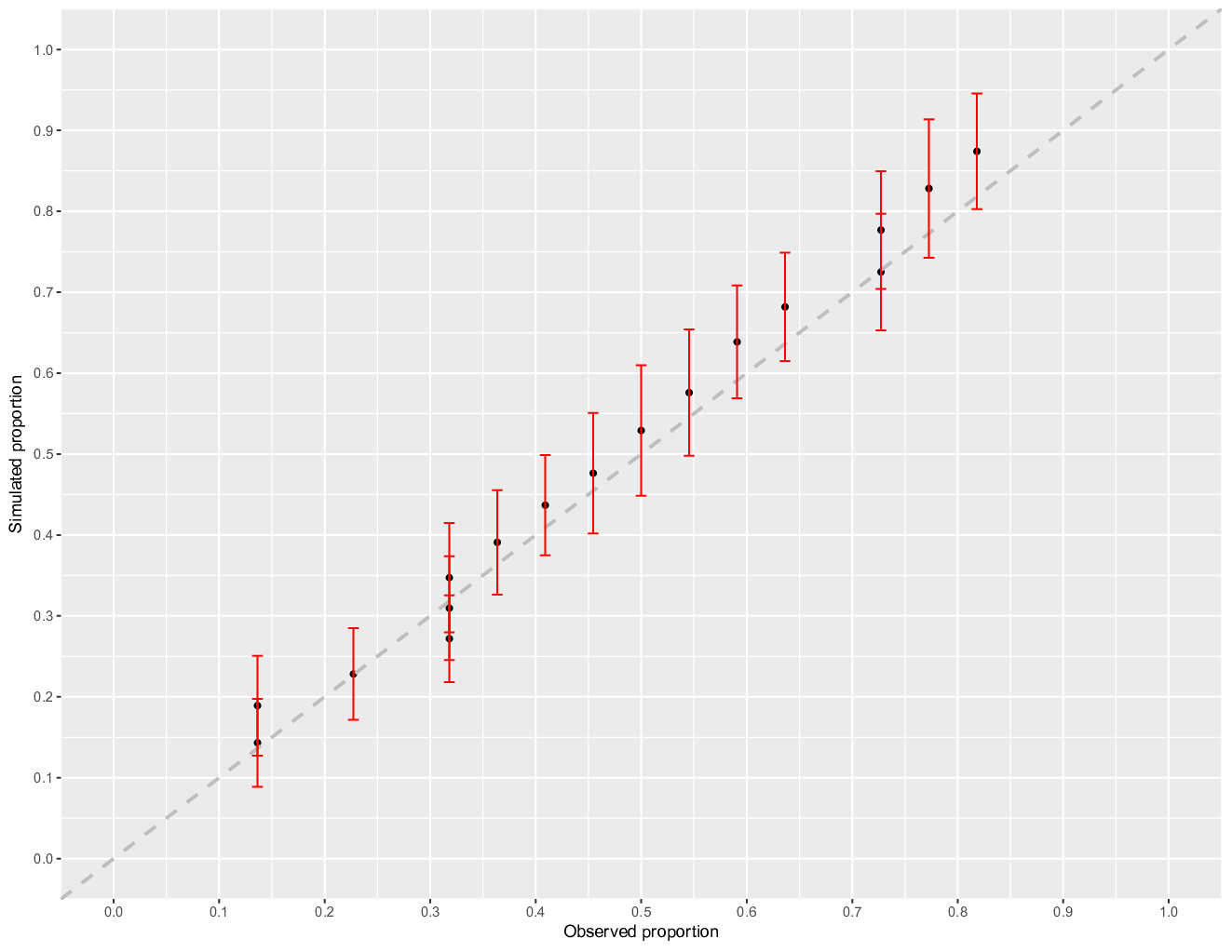
Note: Left panel: Q-Q plot for the simulation study without unobserved confounders. Middle panel: Q-Q plot for the average SIP estimates based on real-world data. Right panel: Q-Q plot for the SIP estimates for subject ID = 311031 based on real-world data.
4 Conclusion
Unobserved confounding is a long-standing issue in causal inference using propensity score methods. Extended from the prior research on this topic, we have proposed nonparametric indices to quantify the impact of unobserved confounders through pseudo-experiments. The numerical studies suggest that the proposed indices can reflect the true impact of these confounders. The application to the real-world data provides a way to identify sufficiency or insufficiency of the observed confounders.
The pseudo-experiments are based on the assumption that the unobserved confounder is similar to some of the observed ones. This assumption can be restrictive in practice. One possible improvement is to conduct sensitivity analysis by simulating some different confounders to study their impact. It will also be interesting to develop test statistics based on the proposed indices. One possibility is to compare the derived ones vs the ones from the null. Another caveat is that although the proposed indices are robust, they may not be sensitive to detect potential confounders. One possible modification is to build some parametric or semiparametric models of the empirical indices and then evaluate the extremity under those models.
In sum, this study is one step forward to address the unobserved confounding issue in causal inference. Despite a few caveats and limitations, it is hoped that this study will stimulate further discussion on this critical issue and help move the science of causal inference forward.
References
- Arah et al. (2008) Arah, O. A., Chiba, Y., and Greenland, S. (2008). Bias formulas for external adjustment and sensitivity analysis of unmeasured confounders. Annals of Epidemiology 18, 637–646.
- Brumback et al. (2004) Brumback, B. A., Hernán, M. A., Haneuse, S. J. P. A., and Robins, J. M. (2004). Sensitivity analyses for unmeasured confounding assuming a marginal structural model for repeated measures. Statistics in Medicine 23, 749–767.
- Carnegie et al. (2016) Carnegie, N. B., Harada, M., and Hill, J. L. (2016). Assessing sensitivity to unmeasured confounding using a simulated potential confounder. Journal of Research on Educational Effectiveness 9, 395–420.
- Fogarty (2019) Fogarty, C. B. (2019). Studentized sensitivity analysis for the sample average treatment effect in paired observational studies. Journal of the American Statistical Association pages 1–13.
- Frank (2000) Frank, K. A. (2000). Impact of a confounding variable on a regression coefficient. Sociological Methods and Research 29, 147–194.
- Groenwold et al. (2010) Groenwold, R., Nelson, D., Nichol, K., Hoes, A., and Hak, E. (2010). Sensitivity analyses to estimate the potential impact of unmeasured confounding in causal research. International Journal of Epidemiology 39, 107–117.
- Hsu and Small (2013) Hsu, J. Y. and Small, D. S. (2013). Calibrating sensitivity analyses to observed covariates in observational studies. Biometrics 69, 803–811.
- Kahlert et al. (2017) Kahlert, J., Gribsholt, S., Gammelager, H., Dekkers, O. M., and Luta, G. (2017). Control of confounding in the analysis phase–an overview for clinicians. Clinical Epidemiology 9, 195.
- Kestenbaum (2009) Kestenbaum, B. (2009). Methods to control for confounding. In Epidemiology and Biostatistics, pages 101–111. Springer.
- Li et al. (2011) Li, L., Shen, C., Wu, A. C., and Li, X. (2011). Propensity score-based sensitivity analysis method for uncontrolled confounding. American Journal of Epidemiology 174, 345–353.
- Lin et al. (1998) Lin, D. Y., Psaty, B. M., and Kronmal, R. A. (1998). Assessing the sensitivity of regression results to unmeasured confounders in observational studies. Biometrics 54, 948–963.
- McCandless et al. (2007) McCandless, L. C., Gustafson, P., and Levy, A. (2007). Bayesian sensitivity analysis for unmeasured confounding in observational studies. Statistics in Medicine 26, 2331–2347.
- McCandless et al. (2008) McCandless, L. C., Gustafson, P., and Levy, A. (2008). A sensitivity analysis using information about measured confounders yielded improved uncertainty assessments for unmeasured confounding. Journal of Clinical Epidemiology 61, 247–255.
- Pan and Bai (2015) Pan, W. and Bai, H. (2015). Propensity score analysis: Fundamentals and developments. The Guilford Press, New York, NY.
- Pan and Bai (2016) Pan, W. and Bai, H. (2016). A robustness index of propensity score estimation to uncontrolled confounders. In Statistical Causal Inferences and Their Applications in Public Health Research, pages 91–100. Springer.
- Pan and Bai (2018) Pan, W. and Bai, H. (2018). Propensity score methods for causal inference: An overview. Behaviormetrika 45, 317–334.
- Pan and Frank (2003) Pan, W. and Frank, K. A. (2003). A probability index of the robustness of a causal inference. Journal of Educational and Behavioral Statistics 28, 315–337.
- Pearson (1895) Pearson, K. (1895). Contributions to the mathematical theory of evolution. ii. skew variation in homogeneous material. Philosophical Transactions of the Royal Society of London 186, 343–424.
- Pourhoseingholi et al. (2012) Pourhoseingholi, M. A., Baghestani, A. R., and Vahedi, M. (2012). How to control confounding effects by statistical analysis. Gastroenterology and Hepatology from Bed to Bench 5, 79.
- Rosenbaum and Rubin (1983a) Rosenbaum, P. R. and Rubin, D. B. (1983a). Assessing sensitivity to an unobserved binary covariate in an observational study with binary outcome. Journal of the Royal Statistical Society. Series B (Methodological) 45, 212–218.
- Rosenbaum and Rubin (1983b) Rosenbaum, P. R. and Rubin, D. B. (1983b). The central role of the propensity score in observational studies for causal effects. Biometrika 70, 41–55.
- Rosenbaum and Silber (2009) Rosenbaum, P. R. and Silber, J. H. (2009). Amplification of sensitivity analysis in matched observational studies. Journal of the American Statistical Association 104, 1398–1405.
- Schneeweiss (2006) Schneeweiss, S. (2006). Sensitivity analysis and external adjustment for unmeasured confounders in epidemiologic database studies of therapeutics. Pharmacoepidemiology and Drug Safety 15, 291 – 303.
- Schneeweiss et al. (2009) Schneeweiss, S., Rassen, J. A., Glynn, R. J., Avorn, J., Mogun, H., and Brookhart, M. A. (2009). High-dimensional propensity score adjustment in studies of treatment effects using health care claims data. Epidemiology 20, 512.
- Springer et al. (2002) Springer, J. F., Sambrano, S., Sale, E., Kasim, R. M., and Hermann, J. (2002). The national cross-site evaluation of high-risk youth programs: Understanding risk, protection, and substance use among high-risk youth. monograph series.
- Stürmer et al. (2005) Stürmer, T., Schneeweiss, S., Avorn, J., and Glynn, R. J. (2005). Adjusting effect estimates for unmeasured confounding with validation data using propensity score calibration. American Journal of Epidemiology 162, 279–289.
- VanderWeele and Arah (2011) VanderWeele, T. J. and Arah, O. A. (2011). Bias formulas for sensitivity analysis of unmeasured confounding for general outcomes, treatments, and confounders. Epidemiology 22, 42–52.
- VanderWeele and Ding (2017) VanderWeele, T. J. and Ding, P. (2017). Sensitivity analysis in observational research: Introducing the e-value. Ann Intern Med 167, 268–274.
- Wang and Krieger (2006) Wang, L. and Krieger, A. M. (2006). Causal conclusions are most sensitive to unobserved binary covariates. Statistics in Medicine 25, 2257–2271.
- Zhao (2019) Zhao, Q. (2019). On sensitivity value of pair-matched observational studies. Journal of the American Statistical Association 114, 713–722.