Test Scene Design for Physically Based Rendering
Abstract
Physically based rendering is a discipline in computer graphics which aims at reproducing certain light and material appearances that occur in the real world. Complex scenes can be difficult to compute for rendering algorithms. This paper introduces a new comprehensive test database of scenes that treat different light setups in conjunction with diverse materials and discusses its design principles. A lot of research is focused on the development of new algorithms that can deal with difficult light conditions and materials efficiently. This database delivers a comprehensive foundation for evaluating existing and newly developed rendering techniques. A final evaluation compares different results of different rendering algorithms for all scenes. The full data set can be downloaded from Zenodo11 1 https://zenodo.org/, 10.5281/zenodo.4002021 and individual scenes can be accessed via a dedicated web repository22 2 https://odpr.cg.tuwien.ac.at.
1 Introduction
1.1 Motivation
Physically Based Rendering (PBR) is a discipline in computer graphics that aims at producing images that resemble the real world as accurate as possible. PBRis integral to photorealism in movies and games as well as architectural and industrial visualization.
In general, the techniques of PBRaim to simulate the lighting conditions as they appear in reality. Therefore, rendering such images requires simulation of light, which is often computationally expensive and time consuming. Generally, PBR consists of several techniques that have to play together to achieve a realistic image, most importantly path tracing and associated Monte Carlo Integration are fundamental methods for creating such images. [PJH16]
Different Monte Carlo-based algorithms exist to render physically correct images, each of them having advantages and drawbacks depending on the scene setup. Research work is focused to improve the efficiency of Monte Carlo Rendering. Newly developed approaches need to be compared and evaluated against already existing ones. The problem is that there are many different scattered scenes available but there is no commonly used database for evaluation and testing, this makes it difficult to compare methods.
The goal of this paper is to deliver a step towards a more consistently designed scene database for the evaluation of different aspects of PBR and Monte Carlo Rendering. Since there can be considerable differences in efficiency and capabilities between the different algorithms, the scenes are designed to include a variety of challenging cases that try to enhance and show the characteristics of such algorithms.
This paper will discuss the individual test scenes and the underlying design principles and also includes rendered examples using a selection of different algorithms. Additional sections regarding Monte Carlo (MC)rendering are included in the appendix. The next section will give an overview of existing test scene databases and related work.
1.2 Related Work
The database described in this paper lays a comprehensive foundation for testing light and material phenomena. For further testing with more complex models, material, and light setups, refer to the PBR database created and gathered by Morgan McGuire [McG17]. It contains several complex scenes with large amounts of polygons as well as a variety of different materials and light setups.
Another comprehensive and more complex database was created and gathered by Benedikt Bitterli [Bit16]. This database contains 32 different scenes ranging from simple scenes to complex scenes with complex light setup and 3D objects. Partially overlapping scenes can be found in the PBRdatabase by Wenzel et al. [MP18]. This dataset features extensive representations of outdoor vegetation with a variety of unique plant models as well as scenes with large portions of glass materials.
An initial approach on scene creation for Global Illumination can be found in the paper Global Illumination Test Scenes by Smits et al. [SJ01]. The scenes contain elementary 3D objects and monochrome light setups to show basic phenomena of light transport.
An analytical approach on Global Illumination scenes can be found in the paper Testing Monte-Carlo global illumination methods with analytically computable scenes by Szirmay-Kalos et al. [SKKA01], which investigates the correctness of Global Illumination algorithms. Because Monte Carlo Rendering uses random sampling, correct or incorrect results (because of implementation errors) are often not noticeable. As a solution, scenes with known exact solutions are used to verify the algorithms.
Another approach on verification of PBR algorithms can be found in the paper Verification of Physically Based Rendering Algorithms by Ulbricht et al. [UWP06]. This paper discusses several state of the art approaches to verify the correctness of light transport simulation as well as advantages and disadvantages of them.
The database discussed in this paper, in contrast, should give a more structured and comprehensive set of test scenes used to observe a variety of phenomena in PBRwithout focus on physical or analytical correctness. Moreover, the modular library containing the 3D objects delivers the possibility to adjust the existing scenes or even create completely new ones.
2 Scene Database
2.1 Introduction
In this chapter, the main motivation of this paper, the creation of a scene database, will be discussed and presented in detail. Twenty scenes were created out of a library of different objects including different lighting situations, simple objects, and more complex objects with different material setups. Since not all algorithms achieve the same result with the same render time, it is interesting to observe the different lighting and material conditions in order to choose an appropriate algorithm that delivers a good result and does not take too long in terms of render time. The evaluation part of this paper will compare render results of different integrators (algorithms like bidirectional path tracing or Metropolis light transport) in terms of render time and visual quality.
The render engine that is used to render the scenes is mitsuba, developed by Jakob Wenzel [Jak10] in 2010. As this is the most common render system for scientific purposes, it is an appropriate choice to observe realistic materials and light conditions and show difficulties and issues common in the field of PBR.
mitsuba is a comprehensive renderer that combines multiple techniques from important research work in Physically Based Rendering. Many inspirations in the system come from the book [PJH16] that was introduced earlier. Important integrators and material properties will be explained later. The material presets are based on real-world measurements according to the mitsuba documentation [Jak14]. The documentation is an extensive collection of all the materials and light emitters that come with the render system, furthermore it contains the usage and constraints of the different components. The scenes have been modeled in Blender 2.79 with the mitsuba plugin. Conveniently, the scenes can be exported as XML file, as the native mitsuba application operates with this file system.
2.1.1 Conceptual Approach
There are several criteria that accompanied the creation of the test scenes. The first and most important one was to design them as representative and expressive as possible. That means that the advantages and drawbacks of the different algorithms can be well distinguished based on the renderings. More specifically, the idea was to use different advanced materials like glass and rough surfaces in order to increase the complexity of the calculations and to challenge the algorithms.
Moreover, the scenes feature typical phenomena/effects characteristic to PBR. However, certain scenes are designed to particularly concentrate on few effects. Refractions and reflections play an important role in realistic synthesized images. Translucent and reflective materials are not perfectly smooth in reality, that means that they have certain surface irregularities. Several scenes feature such surfaces. The difference is that rough materials generally demand more complex calculations, because light scatters more in the scene.
More sophisticated scenes feature materials with Subsurface scattering (SSS), which can only be rendered with a few of the available algorithms. SSSmaterials are considerably relevant to PBR, because – in the real world – many objects are partially translucent. In regard to participating media, some scenes feature atmospheric-like particles, which is a challenge for any algorithm but is also integral to realistic renderings.
Several scenes also feature complex geometry in conjunction with refractive and reflective materials. This will generally challenge the calculations of light paths, especially when it comes to resolving caustics. That is where certain integrators have an advantage compared to basic algorithms like path tracing. Table 1 shows a list with the scenes and the corresponding effects they focus on.
| Scene | RefrSpec | RefrGl | Reflec | Caust | SoftSh | ColBl | PartM | Cgeom | SSS |
| 2.2 | ✓ | ✓ | |||||||
| 2.3 | ✓ | ✓ | |||||||
| 2.4 | ✓ | ✓ | |||||||
| 2.5 | ✓ | ✓ | |||||||
| 2.6 | ✓ | ✓ | |||||||
| 2.7 | ✓ | ✓ | ✓ | ||||||
| 2.8 | |||||||||
| 2.9 | ✓ | ✓ | |||||||
| 2.10 | ✓ | ✓ | ✓ | ||||||
| 2.11 | ✓ | ✓ | ✓ | ||||||
| 2.12 | ✓ | ||||||||
| 2.13 | ✓ | ✓ | ✓ | ||||||
| 2.14 | ✓ | ✓ | ✓ | ||||||
| 2.15 | ✓ | ||||||||
| 2.16 | ✓ | ✓ | |||||||
| 2.17 | |||||||||
| 2.18 | |||||||||
| 2.19 | ✓ | ||||||||
| 2.20 | ✓ | ✓ | |||||||
| 2.21 | ✓ | ✓ | ✓ |
2.2 Scene – Water glass

Figure 1 shows a simple scene with a water glass and a bent mirror. It was made primarily to show complex caustics of the glass material and the mirror. The glass has a common glass material and several indents on the side. The mirror to the right is bent and applied with a copper material preset. The ground has a common metallic material with a high roughness coefficient (see Section 2.3.1). The scene involves a sphere light in the top left of the scene. The sphere light itself is a spherical shape with a material defined as area emitter (see Section 2.2.1), this is a typical setup for any kind of realistic light source in mitsuba.
The glass itself is relatively hard to render because the light that penetrates the glass causes many reflections in several different directions. In order to simulate the real world as accurate as possible, the 3D objects have to have several properties. The glass is defined as an object with an inner material. mitsuba materials allow to set properties for materials that are in the exterior and in the interior (exterior is the side of the normal directions) of the outer boundary. In case of the glass, the exterior is defined as air and the interior as a glass with a typical index of refraction, while the glass material itself is a Smooth dielectric material [Jak14] (see Section 2.2.2). The renderer needs to know these parameters to compute the correct reflection angles, and depending on the preset, the materials have different indices of refraction.
The ground of the scene appears relatively grainy, that is because the surface material has a high roughness coefficient, which means a widespread light scattering in the scene. The scene was primarily designed to test different integrators and to evaluate which of them can handle caustics well. It appears that the caustics coming from the mirror are less grainier than those coming from the glass.
2.2.1 Area Emitter
An area emitter is a light source that emits light via the exterior surface of an arbitrary shape. Unlike some other lights definable in the mitsuba renderer, area emitters generally cast soft shadows. [Jak14]
2.2.2 Smooth dielectric material

Figure 2 shows a geometric interpretation of the Smooth dielectric material in mitsuba. It defines a material with a perfectly smooth surface, that means that the BSDF scatters light in discrete directions (as opposed to rough surfaces with a continuum of resulting light rays). The green arrow in Figure 2 shows the change of direction of the incoming light (red arrow) depending on the index of refraction. The blue arrow shows the portion of the light that is reflected on the surface.
2.3 Scene – Glass pendulum

Figure 3 shows a scene with four glass spheres with a crown glass material preset arranged in a row which is primarily designed to show light propagation through glass materials as well as caustics of spherical shapes. It simulates a light pendulum that transmits the incoming light from the first until the last sphere. An area light connected to a common plane serves as light source. It is slightly raised to have the light direction oriented towards the ground. As a result, the light not only shines straight through the spheres, it also causes the spheres to throw caustics onto the ground. The light propagation of spheres is shown in detail in Figure 6. However, the arrangement of the spheres leads to light being bundled at most for the first sphere. The subsequent spheres gradually receive less light from the previous one. Interesting to observe are the caustics that appear on the ground. They come from the spheres but do not have a typical spherical shape as it is common for such shapes. This comes from the variation of light directly falling on the ground and the intersection with subsequent spheres. This leads to light being refracted in another direction.
A glossy bent mirror is placed behind the pendulum. It has a copper material with little roughness. This is achieved through a Rough conductor material that, unlike the Smooth conductor material, has surface scattering as seen in Figure 4. Interestingly, the ground itself is not as grainy as the ground in Figure 1 although the surface has the same material with equal roughness. This may come from the complexity of the glass portions in the scene and from the shape and intensity of the light source.
2.3.1 Rough conductor material

The Rough conductor material describes a microfacet distribution of a surface. The implementation in mitsuba is based on the paper Microfacet Models for Refraction through Rough Surfaces by Walter et al. [WMLT07]. Microfacets describe surfaces with micro geometry. For instance a metal surface in the real world is not perfectly smooth but it has tiny surface fluctuations. The microfacet model attempts to simulate such surfaces through varying surface normals. The light computation for rough surfaces generally takes longer than for perfectly smooth materials [Jak14].
2.4 Scene – Glass pendulum different shapes

Figure 5 shows a similar scene like before. This time, different shapes are arranged in a row. The light source is a plane emitting from the top left of the arrangement. As different glass shapes throw different caustics, this is an appropriate setup to compare some common shapes. In order to give the light rays an appearance, a participating medium was put around the arrangement. The bounding box of the medium can be seen on the ground where the hard edges appear. The inner surface appears a bit darker because of the light being gradually absorbed/reflected by the particles in the medium. Participating media is good for showing how light rays are cast through space. This can be observed well by looking at the light cones that emerge from underneath the sphere and the glass lens in the middle. The glass cube and the glass bowl have caustics as well but the bundling of the light rays is too weak to appear in the medium, but they can be observed on the ground. The size difference of the light cone of the sphere and the lens is remarkable. This is because of the different diameters. This phenomenon can be seen in Figure 6.

2.5 Scene – Sphere and lenses

The scene in Figure 7 consists of a larger glass sphere and two tinier lenses. The main focus in this scene is to show the properties of light bundling and what shapes are designed to achieve it. The background again features a bent mirror with a Rough conductor material. The light source comes from the top left of the scene. The main focus here is on the light rays that are propagated through the glass materials.
The glass sphere transmits a relatively large amount of the incoming light to the first lens. The lens then casts the incoming portions of light onto the last lens. It is noticeable that the light intensity differs considerably. When looking at the ground to the left of the rendering, it can be observed that due to the transmission and refraction of the light rays through the glass materials, the light gradually intensifies. On the right side of the last lens on the ground, the light intensity is at its peak.
2.6 Scene – Water caustics 1

The scene in Figure 8 was designed to show caustics of waves in a medium like water. An area light is placed on the top and behind the objects. Furthermore, a glass sphere is placed in the middle as well as two diffuse spheres on the sides.
The colored spheres and the walls on the side of the rendering have a Smooth diffuse material [Jak14]. It can be described as a perfectly diffuse material with even distribution of light in any direction (see Section 2.6.1). This material leads to light reflections that are independent from the point of view [Jak14].
Specifically hard to render are the caustics coming from the waves of the water. The colored objects in the scene should help visualize the distribution of the reflected light. Color bleeding resulting from the spheres can be seen underneath the glass sphere. In the real world, there are generally no perfectly smooth diffuse materials, but this was set up out of simplicity.
2.6.1 Smooth diffuse material

The Smooth diffuse material is a surface material that reflects and scatters light independently from the point of view, as seen in Figure 9.
2.7 Scene – Water caustics 2

The scene in Figure 10 shows similar effects like before. A room with a rough diffuse material is filled with water. The water is a deformed plane that simulates waves. Furthermore, a common glass sphere is placed in the middle. On the left there is also a glass prism as well as a glass lens on the right side.
In this case, a participating medium was added for the portions underneath the water surface to show the light rays that are thrown onto the ground. The two colored diffuse spheres in the corners in the background appear less saturated because of the caustics and the participating medium.
Already known are the typical caustics of the sphere in the middle as well as the caustics of the lens. The prism has a more uncommon behavior in respect of light refraction and reflection, regardless, the light rays that are refracted are almost not visible in the medium. This is similar to the scene in Figure 5, where the caustics of the box and the bowl are not visible either, apart from the light that hits the ground.
The portions of the water throwing caustics are larger and more detailed. It is noticeable that the further away the appearances of the caustics are from the light source, the more blurred they become. This can be seen when comparing the caustics directly underneath the surface and the appearances on the ground. Naturally this depends on the edginess of the waves. Relatively choppy waves result in short focal points whereas broad waves result in longer focal points. This is the same principle as it can be observed when comparing the caustics of a lens and a sphere.
2.8 Scene – Color bleeding

The scene in Figure 11 shows a scene set up to show color bleeding, which is a common effect in realistic computer graphics because of the exchange of indirect light between objects in the scene. The idea behind is based on the scene of the cornell boxes from the original paper Modeling the Interaction of Light between Diffuse Surfaces by Goral et al. [GTGB84].
A modification to the original rendering was made in terms of object shapes and the assignment of colors. In this case a green box and a red sphere are placed in front of a mirror on the back wall. The plane area light throws light onto the back side of the box and sphere. This causes the reflections to mainly throw colored reflections onto the back side of the room, which can be seen as green and red reflections around the light source. The mirror on the back wall has little roughness applied so the scattering of the light supports the visualization of color bleeding.
2.9 Scene – Smooth and rough glass

In the scene shown in Figure 12, a high polygon object was used to simulate two different glass materials. The left version has a common glass material with no roughness at all (Smooth dielectric material), whereas the right one has a Rough dielectric material [Jak14] (see Section 2.9.1). The complex object itself has around half a million polygons. A red diffuse sphere was placed inside each of the objects to emphasize the impacts of roughness. On top of each object there is an area light that casts light through the glass.
While the light rays for the Smooth dielectric material reflect in discrete directions, the light rays for the Rough dielectric material scatter in a continuum. On the one hand, the light gets scattered on the exterior of the surface, on the other hand, the light that passes the surface also results in a continuum of scattered light. In case of the rendering, this results in caustics on the ground being more visible for the left object. Additionally, the light that is scattered within the right object is much more present than for the left one because the roughness makes it collect more light inside the surface, specifically visible on the ground.
2.9.1 Rough dielectric material

2.10 Scene – SSScomplex

This scene shows again a complex object slightly modified by adding fissures all over it. The material is designed to show the properties of an SSSmaterial. In order to apply SSSin mitsuba, the base material has to be either a Smooth plastic material or a Rough plastic material. In case of the scene in Figure 14, the material is a Smooth plastic material, which is more complex than the materials used so far (see Section 2.10.1). With SSS, materials like porcelain or wax can be simulated. Typically, light shining on such objects not only reflects it directly on the surface but it also lets portions of light through the surface. The inner medium of the object can be adjusted to have different scattering and absorption coefficients as well. This can be used to control how much light eventually shines through the object. It is clear that, the more solid an object is the less light will appear on the other side. To emphasize the effect of an SSSmaterial, an area light is placed behind the object. It can be seen that portions of the object are considerably bright because the thickness at this location is low.
Mentionable is that SSS can be simulated in two ways in mitsuba. The first one is an approximation (see Section 2.10.2) of the medium that normally is in the interior of the object. The second option is to actually set a participating medium in the interior of the object. The main advantage of the approximation method is a better performance but at costs of accuracy. Participating media is the preferable option to simulate real SSS, but it usually has a higher render time.
2.10.1 Smooth plastic material

The Smooth plastic material simulates a surface with a subsurface, as seen in Figure 15. It simulates a diffuse surface with a dielectric coating surrounding it. As a result, there are generally many internal scattering events. On the one hand, the light gets reflected (blue arrow) when it hits the dielectric coating, on the other hand, the remaining portion of the light (black arrow) goes through the surface and hits the diffuse base layer. This triggers the internal scattering process (green arrays and arrows within the subsurface). [Jak14]
2.10.2 Dipole-based subsurface scattering model
This SSSmodel is implemented in mitsuba and has its origins in radiative transport [EVNT01] and medical physics [Pl12]. The implementation is based on the article A practical model for subsurface light transport by Jensen et al. [JMLH01]. [Jak14]
The Smooth plastic material (see Section 2.10.1) in conjunction with the Dipole-based subsurface scattering model, an approximate simulation of SSScan be achieved. This is done by setting the diffuse reflectance parameter of the plastic material to zero and have the dipole plugin calculate the diffuse part instead. [Jak14]
2.11 Scene – SSScomplex and water

The scene in Figure 16 is a modified version of the scene in Figure 14. This time, a simulated water outflow has been placed above the complex object. The idea behind it is to observe how light behaves in combination with water and a subsurface material underneath. An area light is placed behind the complex object as well.
Since the scene contains only materials with zero roughness – apart from the ground – the light processing is relatively straight forward and simple to render. This is the reason why there is almost no grain in the rendering compared to other scenes. The water itself has a relatively low resolution in terms of polygon count to simplify the scene. Regardless, the water appears fairly realistic although the viscosity of the water seems to be higher, which is rather atypical. Also mind the little caustics in the bottom right corner coming from the water slipping off of the object surface. Because only a few integrators are able to render scenes containing subsurface materials, caustics are often difficult to render. This problem will be treated more detailed later on.
As an example, this scene has been rendered with the common path tracer integrator. This integrator usually has troubles rendering caustics and therefore integrators like bidirectional path tracer are commonly used. The issue with the bidirectional method is that it cannot handle SSSmaterials in mitsuba [Jak14], as this is the case in this scene.
2.12 Scene – Lens light transmission

The scene in Figure 17 shows a setup designed to show the effects of applying a different thickness to convex lenses. Two light sources are placed in the top left corner and in the bottom left corner.
To catch as much light as possible, the light sources are surrounded by geometry, this makes it possible to control the size of the light cone. The first lens in the top left portion of the rendering receives almost all of the incoming light from the top light source. As the lens propagates the incoming light rays onto the bent mirror in about the middle part of the rendering, the rays once more get bundled to construct a relatively narrow focal point. The straight mirror at the mid top receives the scattered light from the bent mirror and reflects it towards a lens with a higher thickness. It is noticeable that the light reaching the last lens is already considerably low. Regardless, the lens bundles the light once more to throw a caustic with a slightly higher light intensity onto a high polygon object, which shows the effect of a convex lens with a higher thickness.
The lens in the bottom left corner and the corresponding mirror on the right side is built to transfer light towards the side of the last lens that is described above. This results in several tiny transmitted rays emerging from the top right of the lens and converging towards the top right of the rendering. Interesting to observe are the considerably long focal points of the lights rays transmitting the lens. The color from the light being reflected by the bent mirror is destined to show clearly what portions of the light get reflected to what location. In order to achieve light rays appearing in a scene, again a participating medium was setup to facilitate this intent. Considerably interesting are the caustics resulting from the bottom left lens, since it appears to throw a variety of light rays from different directions.
2.13 Scene – The lens effect

Figure 18 depicts the effect of glass lenses with different thicknesses. The left one is a bit thicker than the right one, which results in a different magnification and focal point. Previously we have seen the effect in the shape and form of caustics. This time, a more direct approach was taken to show how lenses manipulate incoming light.
The thicker lens to the left appears to magnify the objects in the back more than the right one. Considering the graphical interpretation of light passing through a lens in Figure 6, this means that it depends on the shape, the thickness, and the curvature of the lens, how much the light will be refracted. This leads to the effect that images in thicker lenses appear bigger in size. It is recognizable that the objects placed along the borders of the lenses appear deformed. The thicker the lens, the more distorted objects become around the borders.
2.14 Scene – Double mirrors

The scene in Figure 19 was primarily designed to show the effect of the path depth parameter in the mitsuba integrators. The path depth parameter is a general parameter that can be adjusted for any integrator. The amount of the bounces control how many ray intersections happen per pixel (path depth). This can be observed in the rendering, the scene was rendered using a depth of 32 to show the effect of maximal path depth. This fact is noticeable when looking at the tiny black shaded square located in the mirror towards the top of the rendering. This indicates that the algorithm stopped computing and no further light is processed here. If the path depth is high enough or Russian Roulette is employed, the unfilled area in the mirror would eventually get fully resolved.
Russian Roulette is a Monte Carlo technique used for reducing variance originally introduced by Kirk et al. [AK90]. Basically it stops tracing rays if there is less than a minimum of contribution to the pixel value. [PJH16]
Additionally, a high polygon object with a gold material preset has been placed to increase the complexity of the scene. Furthermore, two convex lenses are placed around the door to increase light complexity. The room itself consists of a door that is slightly opened. Outside the room, an area light is located to emit light towards the door crack as well as an area light inside the room which can be seen in the first mirrored instance. Usually, light coming from a tiny crack is difficult to catch for certain integrators because randomly shooting a ray towards the crack and light source is rare (Path tracer has difficulties resolving such lighting situation). The rough diffuse material of the room increases the complexity of the scatterings as well.
2.15 Scene – Glass Prism

Figure 20 shows a scene set up to describe the behavior of light falling onto a glass prism. The initial idea was to evaluate the correctness of light being refracted and reflected depending on the wavelengths of physical light. Although mitsuba has an option to involve physical light with a discrete set of the wavelength spectrum, this paper and specifically this scene does not observe the behavior of different wavelengths, because the application would need some parameters changed and recompiled to enable this property. Furthermore, a vertical row of spheres is placed inside the prism to produce additional light reflection and refraction. It may appear as if the light rays pass through some participating medium, but the illuminated areas on the ground simply come from the direct and indirect light. At the right hand side of the rendering there is a convex glass lens stuck in the ground, which collects the incoming light and throws a variety of caustics.
Regardless, interesting refractions and reflections of light can be observed in the scene. Like in the previous lens test scene, a light with high intensity was placed on the left side. It is also surrounded by geometry that helps the light shine in a narrower cone than usual. It is noticeable that one portion of the light gets reflected on the first intersection with the prism surface and the other portion gets transmitted through the glass material. Also mind the direction the whole bundle of light rays take when passing through the prism. The glass material has a typical index of refraction of 1.49, which is around an index of crown glass. The arrangement of the spheres in the middle of the prism have a focusing effect on the rays. The light bundle exiting the prism would normally have a lower intensity, since the spheres bundle the rays in the prism, the light appears brighter. Furthermore, it can be slightly seen that the glass spheres cast the typical sphere caustics. Considerably interesting are the caustics thrown from the lens on the right side.
2.16 Scene – Shadows of different light sources

The scene in Figure 21 is designed to show the differences between the most common light sources in mitsuba. The first one is a common area light in form of a sphere, the middle one is a spot light, and the last one is a directional light typically for the sun.
Because of the properties of area lights defined in mitsuba, this type of light source leads to objects casting soft shadows [Jak14]. This is noticeable when observing the darkest portions of the shadows of the objects. The sharpness of the shadow boundary is dependent on the distance to the casting object. Close to the object the shadow boundary is sharp and further away it is more blurred. The same behavior can be seen for the other objects, whereas the area light shadow for the cylinder is barely visible because of the other lights overlapping it.
The spotlight is defined to have a certain linear falloff for the intensity [Jak14], however since the light emits from a single point in space, this type of light source does not cast soft shadows. This can be seen in the rendering when observing the blue light falling onto the objects. The shadows construct a perspectively distorted shape but the sharpness of the shadows remains constant.
The third light (green tint) is a direct light emitter, as defined in mitsuba [Jak14]. Typically, it simulates the sun like it exists in reality, which emits light rays in a specific direction. The common effect of a light source like the sun can be seen in the rendering by observing the shadows that the green light casts. Particularly, the shadows from the sphere and the cylinder appear to have a constant shape over distance. Soft shadows do not occur for this type of light source either.
Another interesting aspect is the difference of the materials of the objects. Whereas the complex object left has almost no grain, the red diffuse sphere and the rough metal cylinder exhibit a large amount of it as well as the shadows. This is because of the complexity of the surface material. The complex object has a smooth material, which makes it easier to render, whereas the red sphere and the cylinder have a diffuse material with moderate roughness that scatters the light to a greater extent.
2.17 Scene – Light from slightly opened door

The scene in Figure 22 was specifically made to test the behavior of light coming from a door that is almost closed. The idea behind it was to observe a variety of soft shadows being cast all over the scene and to have a relatively simple setup of materials that simultaneously lead to a quick convergence and a visually pleasing result. The glass and mirror materials in the scene do not have any roughness, this is to decrease complexity overall and to put the focus on the light distribution through the door. The scene was rendered with the same amount of spp(1024) as most of the other scenes, yet the result is already considerably good compared to other renderings. This is also because of the perfectly smooth glass and mirror surfaces. Several grainy portions can be observed on the right side of the cube where the light source from the door appears and on the back side of the sphere when looking at the right mirror. Interesting to observe are the cube shadows cast on the left wall on the left hand side of the rendering.
2.18 Scene – Light from outside

The scene in Figure 23 is, similarly to previous scene, designed to show soft shadows and glass materials. This time the light comes from a window involving a shutter object that breaks and scatters the incoming rays. Additionally to an area light in form of a plane placed outside the window, the world environment is set to have a constant monochrome light. This can be seen when looking at the right-hand side around the window. The bright brownish light that appears on the back wall comes from the area light source.
The effect of the decreased sharpness of soft shadows over distance can be distinctly seen when looking at the light projections at the back wall. Apart from the shadows getting more blurred, the further the light travels also the intensity of the reflected light gradually decreases. It is noteworthy that the light intensity in the mirror on the left side is higher than the intensity directly on the back wall. This happens because of the specularity of the room. The roughness is considerably high but is not independent from the point of view. The light reflecting from the diffuse back wall gets reflected by the mirror, which eventually reflects it back to the camera with a higher intensity. This is due to the angle towards the light source and therefore an angle that is closer around the perfect reflection angle of the wall.
A high polygon model is located on top of the cube. It is noteworthy that the graininess of the complex model differs considerably compared to the glass cube. There are more reflections outside and inside the high polygon object and therefore the scene is more difficult to render. Compared to the scene before (see Figure 22), this one has also been rendered with PSSMLTwith 1024 samples per pixel. Yet, the scene overall looks more grainy also because of the higher light intensity coming from outside.
2.19 Scene – SSSand realistic light setup

The scene in Figure 24 was specifically designed to show behavior of large portions of materials with SSSin a more realistic light setting. Therefore, two high polygon objects are placed in the scene, one is a simulated wax candle and the other is the known high polygon object from previous scenes. The candle wick is lit and supports to show the impact of light on the subsurface material. Typically for candles, the light goes through the top of the lit surface and gradually decreases towards the bottom.
The light source coming from outside is a constant environment tinted slightly blueish. This should simulate indirect environment lighting. Additionally to the light from outside, a lamp in the room was placed above the objects to give the scene more depth and several light scatterings.
Hard to render are the glass spheres located inside the water glass. They have a glass material with a moderate roughness, and therefore the graininess for this portion of the rendering is considerably high compared to the rest of the image.
2.20 Scene – Complex SSSand rough glass surfaces

Figure 25 shows a scene with several different materials put together. Generally, this scene was designed with a more artistic and more complex approach in mind. The cloth blanket that covers objects underneath has an SSSmaterial applied to simulate more realistic clothing. The high polygon object to the left has a gold material applied. Underneath the blanket, in the middle of the scene, there is a glass box with a red diffuse sphere inside and the object to the right is a water glass. Behind in the back of the scene, a mirror with moderate roughness distributes the light that shines onto the blanket from behind. Another light is placed above to allow the water and lenses to throw visible caustics. Additionally to these objects a water outflow was put above the scene mainly to let the water throw caustics on the ground. Another rough glass sphere is placed on top of the glass to the right to emphasize light scattering inside the blanket. In that respect, it is also noticeable that the bottom of the blanket is highlighted from the scattered light inside.
The scene was rendered with the Extended volumetric path tracer (volpath) [Jak14] integrator. Also mind the relatively sharp and smooth portions of the rendering that do not belong to glass caustics. This is a well known problem for volpath. Yet, for 1024 samples per pixel, the caustics on the bottom of the image coming from the water drops and the lens are considerably good but still grainy in comparison when rendered with an integrator like PSSMLT. It is noticeable for the blanket that there are several cloth folds that generally receive less light from the internal scattering events and therefore convey a better perception of depth. Also interesting is to show SSSwith parameters that are typical for cloth and how little is visible through the highly scattering material.
2.21 Scene – Water caustics and broad light distribution

The scene in Figure 26 is a constellation of objects with different materials arranged around an area light in form of a sphere. Starting with the first object, a bent mirror with a slightly rough copper material is placed behind the sphere light to enable diffuse light scatterings. On the left side, a red diffuse sphere within a larger glass sphere is placed. To give the scene a more complex material setup, a wax candle with an SSSmaterial was added. Besides the high polygon wax candle, the raven head was added as well and has been applied with a gold material. The last object is a simple cylinder with a metal texture with moderate roughness.
Additionally, a water mesh fills the room so about half of the height of the objects are located inside. It is noticeable that for the red sphere, the reflection of the light source is not as intense. This comes from a light portion getting reflected by the outer glass sphere and the other portion hitting the red diffuse material. The roughness of the bent mirror ensures that there are many light scattering events that take place over the scene. This increases complexity in terms of rendering time and visual quality. The volpath integrator has been used to render the image. The issue is that the scene has an SSSmaterial and simultaneously there are many caustics that need to be rendered. This leads to the problem that integrators like PSSMLTwould not work because of the implementation in mitsuba. The deficit of volpath not being able to handle caustics well, is noticeable when looking at the darker portions of the rendering. The perceivable variance is very high and the image as a whole looks very grainy.
3 Evaluation
This chapter deals with the evaluation of the scenes that are described in Chapter 2. Depending on the scene, the integrators achieve considerably different results within the same render time. Each scene evaluation will contain five (four in special cases) render results from a selection of the most relevant integrators. The algorithms partially sample light very differently and comparing on the basis of equal sppwould hide the sampling overhead of the different algorithms. This is the reason why the results from the renderings are compared with render time. Perfectly accurate consensus in render time is not possible, but the differences in time are around plus/minus ten seconds.
3.1 Integrators
The following will give brief descriptions about the integrators as well as the abbreviations that are used in the evaluation.
Path tracer (PT)
The Path tracer is a basic path tracer implementation that shoots random rays from the camera into the scene. It is a good choice when the scene contains only simple lighting with no obstacles along the light paths. [Jak14]
It uses Multiple Importance Sampling to reduce variance in the image. Multiple Importance Sampling is a technique in Monte Carlo-sampling that uses the idea of taking samples from multiple different probability density functions (like described in Section A.2.5), in the hope that one of the distributions resembles the shape of the integrand. [PJH16]
Simple volumetric path tracer (VOLPATH SIMPLE)
The Simple volumetric path tracer implements a basic volumetric path tracer that is used to render volumes in scenes (participating media, SSSmaterials). It does not make use of Multiple Importance Sampling. [Jak14]
Extended volumetric path tracer (VOLPATH)
This integrator implements a volumetric path tracer and it also uses Multiple Importance Sampling. In respect of surfaces, it behaves like the standard Path tracer [Jak14]
Bidirectional path tracer (BDPT)
The BDPTis implemented as proposed by Veach and Guibas [VG95], in conjunction with Multiple Importance Sampling. The basic idea is to start two random ray paths in one step. One ray starts from the camera and one from an emitter as described in Section A.2.5. BDPTusually is considerably slower than Path tracing for the same amount of samples but generally results in images with much less perceivable variance. [Jak14]
Photon mapper (PM)
The Photon mapper implementation is based on the idea proposed by Jensen [Jen96]. The calculation of light is separated into three classes. Diffuse, caustic, and volumetric maps are built separately. A ray tracing pass follows that estimates the radiance using the photon maps.
Progressive photon mapper (PPM)
This integrator implements Progressive photon mapping by Hachisuka et al. [HOJ08]. It is based on Photon mapping but it progressively calculates and shows the results as the passes continue indefinitely until eventually all variance vanishes.
Stochastic progressive photon mapper (SPPM)
This integrator implements SPPMas proposed by Hachisuka et al. [HJ09]. It is an extension of Progressive photon mapping that has better performance when it comes to motion blur, depth of field or glossy reflections.
Primary Sample Space Metropolis Light Transport (PSSMLT)
This rendering technique was developed by Kelemen et al. [KSK01], based on Markov Chain Monte Carlo Integration [Has70]. Usually, algorithms like path tracing compute images by randomly shooting light paths into the scene. PSSMLTbenefits from the fact that it tries to find most relevant light paths. If a relevant path is discovered also neighbored paths are evaluated and involved in the calculation. Generally, this improves the render time considerably and complex light situations give a better result. [Jak14]
Metropolis Light Transport, Path Space Metropolis Light Transport (MLT)
MLTis similar to PSSMLT. Both integrators search for light paths that carry a high amount of light energy. PSSMLTdoes this by using another rendering technique. MLTinstead works directly on the light carrying paths and therefore has more information available. This allows directed search for certain classes of light paths. [Jak14]
Energy Redistribution Path tracing (ERPT)
This integrator by Cline et al. [CTE05] uses Path tracing in conjunction with techniques of Metropolis Light Transport. With the use of a standard bidirectional path tracer, a set of seed paths is generated. An MLTMarkov Chain is then started for each path that redistributes the energy of the samples over a larger area.
Irradiance caching (IRRCACHE)
Irradiance caching is a meta-integrator that works on top of other integrators. It was developed by Ward and Heckbert [WRC88]. It calculates and caches irradiance information at several scene locations and fills the other locations through interpolation. This can be helpful if results would otherwise look blotchy (often used with photon mapping).
3.2 Water glass

The reference in Figure 27 was rendered with PSSMLTwith 2048 samples per pixel (spp). The result of the path tracer (PT) integrator was used as a benchmark in terms of render time. The images where rendered in about 1.6 minutes. Concerning soft shadows (bottom row), PT had difficulties delivering good results. BDPTresulted in considerably lower perceived variance. PSSMLTand PMalso had difficulties rendering soft shadows and resulted in a lower visual quality than BDPT. The best results were achieved by ERPT.
The glass portions (Figure 27 middle and top row) of the scene are hard to render. Both PTand BDPThad troubles resolving these parts. PSSMLTand ERPTachieved the best results while PMdelivered a result that is too dark overall. However, PMresolved the caustic on left side of the glass (on the ground) better than the other integrators. This can be seen in Figure 27 PMtop row, it shows considerably less perceivable variance than the other results.
3.3 Glass pendulum

The reference in Figure 28 was rendered with PSSMLTwith 1024 samples per pixel. All comparison images were rendered in 1.3 minutes. The PThas problems resolving the caustics that are thrown by the spheres. Also the bent mirror in the background (which has little roughness) has a considerably high perceivable variance. While the BDPTachieves good results on the portions of the ground (shadows and caustics) the bent mirror also has a high perceivable variance and is not visually better than the result from PT.
PSSMLTresolves all aspects better than the other integrators. MLTand ERPTresolve the ground similarly like PSSMLTbut have problems rendering the bottom part of the bent mirror (Figure 28 top row). This can be seen as little light peaks all over the bottom of the mirror.
3.4 Glass pendulum different shapes

The reference in Figure 29 was rendered with PSSMLTwith 1024 samples per pixel. The comparison images were rendered in 1.6 minutes. The BDPTrendered the scene considerably well. If compared to the result from PSSMLT(which achieved the visually best result), there is not much difference. Little drawbacks can be seen in terms of higher perceivable variance for the BDPT.
VOLPATH SIMPLEdid not achieve good results, the integrator had issues finding the light carrying paths as well as light scattered inside the volume of the participating medium. The PMdid not work well, it did not catch the caustics on the ground and it had problems resolving scattered light inside the volume. The results from ERPTare behind PSSMLTand BDPTbecause the perceivable variance is even higher but it resolves the caustics and volume visually better than PMand VOLPATH SIMPLE.
3.5 Sphere and lenses

The reference in Figure 30 was rendered with PSSMLTwith 1024 samples per pixel. The comparison images were rendered in 2.0 minutes. Like in the previous scenes, the PThas issues resolving caustics and in general light paths that are considerably complex. This results again in high perceivable variance all over the scene. The BDPTachieves relatively smooth results on the ground portions but not for the bent mirror in the background (more grainy).
PSSMLTagain achieves the visually best result among all integrators although MLTresolves the lenses a bit better (Figure 30 MLTmiddle row). MLThas several light phenomena/caustics that are not present in the reference image. While ERPTdoes a good job for the lenses and ground portions, it does not resolve the bottom of the mirror, neither does MLT.
3.6 Water caustics 1

The reference in Figure 31 was rendered with PSSMLTwith 1024 samples per pixel. The comparison images were rendered in 2.6 minutes. The scene lighting in conjunction with the waves on the ground makes this scene difficult to render. The PTachieves results with high perceivable variance. However, in comparison to the BDPTit occurs to resolve light paths better.
PSSMLThas little issues and resolves the caustics relatively well. PMresults in a considerably darker scene when trying to catch the light and caustics from the water, all other parts (the diffuse spheres) are similar to the other results. ERPTachieves the best result when it comes to caustics even though there are light artifacts all over the water, however, the caustics generally exhibit less perceivable variance than for PSSMLT.
3.7 Water caustics 2

The reference in Figure 32 was rendered with PSSMLTwith 1024 samples per pixel. The comparison images were rendered in 3.2 minutes. The VOLPATHintegrator did not achieve good results, the noise is very high. The PMwas used with IRRCACHEbut had problems resolving certain parts as well, especially for caustics.
PSSMLThad no problems rendering the scene. The perceivable variance seems to be the lowest among all integrators. MLTresults in appropriate caustics as well on the one hand, on the other hand, it shows many individual light features all over the scene. Also the scene overall looks a bit darker than for the other integrators. ERPTdid not create any artifacts but the perceivable variance seems to be still higher than for PSSMLTand MLT.
3.8 Color bleeding

The reference in Figure 33 was rendered with PSSMLTwith 1024 samples per pixel. The comparison images were rendered in 3.4 minutes. The PTshows high perceivable variance in the resulting image. BDPTas well as PSSMLTdelivered very similar results. BDPTonly had more issues resolving the mirror in the background that shows slightly higher perceivable variance than for PSSMLT(Figure 33 mirror in bottom and mid row).
The PMoverall resulted in an image with high perceivable variance comparable to the result from the PT. The ERPTachieved good results as well and is similar to the results from BDPTand PSSMLT, however, the scene overall looks slightly blurry. To conclude, the BDPTis probably preferable here because it has slight benefits in terms of memory usage compared to PSSMLT.
3.9 Smooth and rough glass

The reference in Figure 34 was rendered with PSSMLTwith 1024 samples per pixel. The comparison images were rendered in 3.5 minutes. The PThad troubles rendering the caustics from the smooth glass object on the left side as well as from the rough glass object on the right side. In both cases, the perceivable variance is higher compared to other integrators. BDPTdid a considerably better job at rendering the caustics. However, it also has the same issues when it comes to rendering the interior lighting of the glass material and exhibits high perceivable variance, especially for the rough glass object.
PSSMLTachieved good results overall. It does well on caustics and the rough glass parts. Yet, the BDPTresolves the caustics a bit better (Figure 34 bottom row). The PSSMLThas a lower perceivable variance for the bottom part of the rough glass (Figure 34 middle row) but the BDPThas a lower perceivable variance for the top part of the rough glass (Figure 34 top row).
The PMexhibits similar perceivable variance like the PTand is not suitable for this scene. The rendering from the ERPThas the lowest perceivable variance for the rough glass object but exhibits artifacts for the smooth glass object on the left side. It seems that PSSMLTachieved the best result overall.
3.10 SSScomplex

The reference in Figure 34 was rendered with the PTwith 1024 samples per pixel. The comparison images were rendered in 2.5 minutes. Only PT, VOLPATH, VOLPATH SIMPLEand PMare able to capture SSSmaterials. The results from the different integrators are almost equal. PT, VOLPATH SIMPLEand VOLPATHachieve the same result in terms of visual quality and memory usage. PMresults in a very similar image but it uses slightly more memory for the calculations.
3.11 SSScomplex and water

The reference in Figure 36 was rendered with PT(Independent Sampler) with 1024 samples per pixel. The comparison images were rendered in 2.8 minutes. Again the PT, the VOLPATHintegrators and PMare able to capture the SSSmaterials in a scene. The results from PT, VOLPATHand VOLPATH SIMPLEhad similar results. One more closeup visual inspection, the PMseems to have achieved the best results overall. It has the lowest perceivable variance and it could resolve the SSSmaterial under the water better than the other integrators.
3.12 Lens light transmission

The reference in Figure 37 was rendered with PSSMLTwith 1024 samples per pixel. the comparison images were rendered in 2.6 minutes. VOLPATH SIMPLEand VOLPATHachieved similar results, both having high perceivable variance overall however. PSSMLT, MLTand ERPThave similar results as well. The most difference can be seen for the complex glass object (Figure 37 middle row) and the thick lens (Figure 37 top row). The results from MLTare generally too dark. The result from ERPThas a better approximation but still has problems resolving the complex glass object. Overall, the PSSMLTachieved the best results.
3.13 The lens effect

The reference in Figure 38 was rendered with PSSMLTwith 1024 samples per pixel. The comparison images were rendered in 2.7 minutes. PT, BDPT, PSSMLTand SPPMachieved very similar results. SPPMdelivered an image that appears sharper than for the other integrators. The results from the PT, BDPTand PSSMLTare slightly blurry. The image rendered with PMis generally too bright and the perceivable variance is high as well. PSSMLThad no advantage for this scene, the light energy is considerably uniform over the scene so PTand BDPTare preferable in terms of memory usage here. SPPMdelivers the best result but also has the highest memory usage.
3.14 Double mirrors

The reference in Figure 39 was rendered with PSSMLTwith 1024 samples per pixel. The comparison images were rendered in 2.8 minutes. As expected, the PThad troubles rendering the scene because of the relatively complex light setup. The perceivable variance is considerably high, as well as for BDPTwhich has the same issues. Yet, BDPTstill exhibits slightly lower perceivable variance than PT. Surprisingly, PSSMLTalso has troubles with the scene and also exhibits considerable variance but still has a better visual quality than PTand BDPT.
The MLTversion was rendered with 300 samples per pixel and stopped when the expected render time was reached. The ground and wall portions of the scene have much less perceivable variance than for the other integrators. However, MLTcould not correctly resolve the interior of the complex glass object (Figure 39 MLTmiddle row). Also it could not resolve the mirror part (Figure 39 top row) like the other integrators. It occurs as if the path depth is too low although it has been rendered with 32 bounces or the MLTdid not have enough time to sample these areas. ERPTachieved a similar visual quality like PSSMLTbut with slightly less perceivable variance overall.
3.15 Glass prisma

The reference in Figure 40 was rendered with PSSMLTwith 1024 samples per pixel. The comparison images were rendered in 2.1 minutes. PT, PMand SPPMhad considerable problems catching light paths in this scene. Especially, in case of PM, the scene looks too dark overall.
The results from the BDPTwere better than for the PT, but the perceivable variance is still high. PSSMLTresolved the ground of the scene and the caustics from the lens relatively well (Figure 40 PSSMLTmiddle row). However, also PSSMLThad troubles resolving the lighting within the glass materials.
3.16 Shadows of different light sources

The reference in Figure 41 was rendered with PSSMLTwith 1024 samples per pixel. The comparison images were rendered in 1.8 minutes. Regarding the objects, especially the red sphere and the metal cylinder (Figure 41 top row), the PTand PMresulted in images with the lowest perceivable variance.
Other than that, the results from all integrators are very similar. Preferable is the PMbecause it has the lowest perceivable variance overall. However, the shadow of the red sphere gets resolved better with ERPT(Figure 41 ERPTtop row) than for the other integrators.
3.17 Light from slightly opened door

The reference in Figure 42 was rendered with PSSMLTwith 1024 samples per pixel. The comparison images were rendered in 3.2 minutes. PTagain exhibits the most overall perceivable variance of all integrators because of the complex light setup (light coming from a door that is slightly opened). BDPTdelivers a better image than PTin terms of variance overall. PSSMLTis comparable to the result from BDPTbut resolves light paths a bit better (less perceivable variance) as seen in Figure 42 in the bottom row.
The PMhad troubles resolving the mirror area which results in regions that are too dark and with high perceivable variance. ERPTresolves the area in the left mirror better than PSSMLT(Figure 42 bottom row). Also the perceivable variance overall is slightly lower with ERPTthan with PSSMLT.
3.18 Light from outside

The reference in Figure 43 was rendered with PSSMLTwith 1024 samples per pixel. The comparison images were rendered in 2.5 minutes. The results are similar to those of the previous scene. PThas little perceivable variance on the wall parts of the room (Figure 43 PTtop and bottom row). BDPThas less perceivable variance than PT. As in the case of the complex glass object (Figure 43 middle row), it resolves the lighting in the interior slightly better than PSSMLT. MLThas troubles resolving the lighting of the interior of the complex glass object as well, even more than PSSMLT. Also MLThas a few outliers (bright blotches like in the middle row on the back wall) spread all over the scene, which are not present for the other results. ERPThas similar results like PSSMLTand BDPTbut exhibits higher perceivable variance for the complex glass object.
3.19 SSSand realistic light setup

The reference in Figure 44 was rendered with PSSMLTwith 1024 samples per pixel. The comparison images were rendered in 2.5 minutes. PT, VOLPATH SIMPLE, VOLPATHand PMhave very similar results. VOLPATH SIMPLEhas slightly more perceivable variance overall than the other results. PMhas problems resolving the glass materials in the scene (Figure 44 PMbottom row), generally they are too dark.
3.20 Complex SSSand rough glass surfaces

The reference in Figure 45 was rendered with VOLPATHwith 1024 samples per pixel. The comparison images were rendered in 3.0 minutes. PTand VOLPATHhas very similar results (because VOLPATHuses PTfor surfaces). The perceivable variance is relatively high for the caustics on the ground coming from the water drops and lenses (Figure 45 middle row). VOLPATH SIMPLEgenerally has very similar results like PTand VOLPATHas well but it has troubles rendering the top of the complex object with the gold material (Figure 45 bottom row), it appears too dark and with high perceivable variance. PMachieved very similar results compared to VOLPATHand PTas well and it has no obvious advantages or disadvantages except from the slightly higher memory usage.
3.21 Water caustics and broad light distribution

The reference in Figure 46 was rendered with VOLPATHwith 1024 samples per pixel. The comparison images were rendered in 2.8 minutes. This scene exhibits difficult light paths so all of the integrators had difficulties rendering the scene. PT, VOLPATH SIMPLEand VOLPATHall show very similar results. However, the scene looks very grainy overall because of the PTnot being capable of finding relevant light paths. The problem is, that an SSSmaterial exists in the scene and it cannot be rendered with integrators like PSSMLTwhich may resolve the light situation considerably better. The IRRCACHEintegrator was used in conjunction with PMas well but did not deliver a better result than the others. The scene looks darker overall and the perceivable variance is high as well.
4 Conclusion
In the previous chapter we have seen that the discussed integrators have different advantages and disadvantages depending on the scene setup. In conclusion, we will recapitulate the most important aspects that came to light in the evaluation chapter.
The PTintegrator generally has problems rendering complex light conditions, this may result in high perceivable variance because the algorithm (randomized rays) has problems sampling important light paths sufficiently. Furthermore, this issue also affects rendering of glass materials and caustics – more advanced integrators like PSSMLTmight be the better choice for that. Interestingly, certain light and material conditions may lead to less perceivable variance than BDPT, as is the case in Figure 31, mainly because PT used far more spp than BDPTand most of the objects have diffuse materials which are easy to render.
In general, BDPThas difficulties rendering translucent materials like glass as well. However, it seems to be the better choice than PT (with exceptions like mentioned before). Under certain light and material conditions, BDPT might come close to the visual quality of PSSMLT, see Figure 42 for an example. Certain conditions can also result in BDPT being able to resolve caustics slightly better than PSSMLTlike in Figure 34.
The PSSMLT integrator generally delivers good results when dealing with difficult light paths, as is the case with translucent materials in conjunction with diffuse surfaces (for example light going through the water surface, hitting the ground and going through the water again until eventually the camera catches the light).
MLT generally delivers similar results like PSSMLT, however, it might also render caustics with less perceivable variance. For smooth glass materials it also generally has advantages in visual quality compared to PSSMLT. As in the case of Figure 30, MLT may deliver results with odd behavior (MLTbottom row) which differ considerably from the other results. Figure 32 also shows that it might result in glass materials appearing darker in the rendering, this might come from the time limitation for the algorithm to converge, a good example concerning this issue can also be seen in Figure 39, where the glass materials are also darker and the mirror part is not completely resolved compared to the other results.
PM often delivers visual quality that is below the results from BDPT in the same render time. Glass materials also seem to be darker than from other integrators (for instance in Figure 31), this may be because of the limited render time. PMconverges to the reference when enough photons are stored in the photon maps, ideally tending to an indefinite amount. As a disadvantage, PM generally requires considerably more memory than other integrators, but it delivers good results if enough time is available to render the scene. PM might not work well for scenes with participating media like in Figure 29.
The ERPT integrator is generally a good choice for scenes, especially for glass materials and complex caustics. However, it has difficulties rendering participating media and its visual quality is below the results from PSSMLT and BDPT. Furthermore, it can result in visually blurry renderings, as in the case of Figure 33. Interestingly, as in the case of Figure 34, the rough glass material appears to have the lowest perceivable variance among the tested integrators, but the smooth glass material appears to have the highest perceivable variance.
VOLPATH SIMPLEand VOLPATH seem to have, in comparison to other integrators like PSSMLT, more difficulties rendering participating media. The difference when rendering SSS(dipole-based subsurface scattering) materials is not noticeable compared to the results from PT or PM like in Figure 35, this is expected because VOLPATHis basically a PT with the possibility to render participating media. SPPMseems not to be a good choice in general, although it might deliver better results in rare cases, like in Figure 38.
The designed scenes for this paper should show where integrators exhibit large differences in the results. Mentionable are the scenes in Figures 29, 30, 31, 32, 34, 39 due to the large variations in the renderings.
The scenes are all available in XML format, they can conveniently be loaded and rendered in mitsuba. Additionally, the Blender files are published, which contain the scene setups and a library containing the linked objects. When adding new objects to a scene, it is preferable to link the blend files instead of appending, so the material parameters can be adjusted from a single point of reference, but the objects can also be made local to test different parameters only in that scene. The scenes have been tested with Blender 2.79b, mitsuba version 0.5.0 and mitsuba Blender plugin version 0.5.1.
Acknowledgments
Research reported in this paper was supported by Austrian Science Fund (FWF): ORD 61
References
- [AK90] James Arvo and David Kirk. In Particle Transport and Image Synthesis, volume 24, pages 63–66, 09 1990.
- [Bit16] Benedikt Bitterli. Rendering resources, 2016. https://benedikt-bitterli.me/resources/.
- [CTE05] David Cline, Justin Talbot, and Parris Egbert. Energy redistribution path tracing. ACM Trans. Graph., 24(3):1186–1195, July 2005.
- [EVNT01] G. Eason, A. Veitch, Roger Nisbet, and F. Turnbull. The theory of the back-scattering of light by blood. Journal of Physics D: Applied Physics, 11:1463, 01 2001.
- [GTGB84] Cindy M. Goral, Kenneth E. Torrance, Donald P. Greenberg, and Bennett Battaile. Modeling the interaction of light between diffuse surfaces. SIGGRAPH Comput. Graph., 18(3):213–222, January 1984.
- [Has70] W. K. Hastings. Monte carlo sampling methods using markov chains and their applications. Biometrika, 57(1):97–109, 1970.
- [HJ09] Toshiya Hachisuka and Henrik Wann Jensen. Stochastic progressive photon mapping. ACM Trans. Graph., 28(5):1–8, December 2009.
- [HOJ08] Toshiya Hachisuka, Shinji Ogaki, and Henrik Wann Jensen. Progressive photon mapping. In ACM SIGGRAPH Asia 2008 Papers, SIGGRAPH Asia ’08, New York, NY, USA, 2008. Association for Computing Machinery.
- [Jak10] Wenzel Jakob. Mitsuba renderer, 2010. http://www.mitsuba-renderer.org.
- [Jak14] Wenzel Jakob. Mitsuba Documentation, 2014. https://www.mitsuba-renderer.org/docs.html.
- [Jen96] Henrik Wann Jensen. Global illumination using photon maps. In Proceedings of the Eurographics Workshop on Rendering Techniques ’96, page 21–30, Berlin, Heidelberg, 1996. Springer-Verlag.
- [JMLH01] Henrik Wann Jensen, Stephen R. Marschner, Marc Levoy, and Pat Hanrahan. A practical model for subsurface light transport. In Proceedings of the 28th Annual Conference on Computer Graphics and Interactive Techniques, SIGGRAPH ’01, page 511–518, New York, NY, USA, 2001. Association for Computing Machinery.
- [Kaj86] James T. Kajiya. The rendering equation. In Computer Graphics, pages 143–150, 1986.
- [KNK+16] David Koerner, Jan Novák, Peter Kutz, Ralf Habel, and Wojciech Jarosz. Subdivision next-event estimation for path-traced subsurface scattering. In Proceedings of the Eurographics Symposium on Rendering: Experimental Ideas & Implementations, EGSR ’16, page 91–96, Goslar, DEU, 2016. Eurographics Association.
- [KSK01] Csaba Kelemen and László Szirmay-Kalos. Simple and robust mutation strategy for metropolis light transport algorithm. Technical Report TR-186-2-01-18, Institute of Computer Graphics and Algorithms, Vienna University of Technology, Favoritenstrasse 9-11/186, A-1040 Vienna, Austria, July 2001. human contact: technical-report@cg.tuwien.ac.at.
- [LW98] Eric Lafortune and Yves Willems. Bi-directional path tracing. Proceedings of Third International Conference on Computational Graphics and Visualization Techniques, 93, 01 1998.
- [McG17] Morgan McGuire. Computer graphics archive, July 2017.
- [MP18] Greg Humphreys Matt Pharr, Wenzel Jakob. Scenes for pbrt-v3, 2018.
- [PJH16] M. Pharr, W. Jakob, and G. Humphreys. Physically based rendering: From theory to implementation: Third edition. Morgan Kaufmann, 11 2016.
- [Pl12] Dong-qing Peng and Hui li. Study for noninvasive determination of optical properties of bio-tissue using spatially resolved diffuse reflectance. Progress in Biomedical Optics and Imaging - Proceedings of SPIE, 8553:30–, 12 2012.
- [SJ01] Brian Smits and Henrik Jensen. Global illumination test scenes. 03 2001.
- [SKKA01] László Szirmay-Kalos, László Kovács, and Ali Abbas. Testing monte-carlo global illumination methods with analytically computable scenes. 02 2001.
- [SKP07] Musawir Shah, Jaakko Konttinen, and Sumanta Pattanaik. Caustics mapping: An image-space technique for real-time caustics. IEEE transactions on visualization and computer graphics, 13:272–80, 03 2007.
- [UWP06] Christiane Ulbricht, Alexander Wilkie, and Werner Purgathofer. Verification of physically based rendering algorithms. Computer Graphics Forum, 25(2):237–255, June 2006.
- [Vea98] Eric Veach. Robust Monte Carlo Methods for Light Transport Simulation. PhD thesis, Stanford University, Stanford, CA, USA, 1998. AAI9837162.
- [VG95] Eric Veach and Leonidas Guibas. Bidirectional estimators for light transport. Proceedings of Eurographics Workshop on Rendering, 01 1995.
- [VG97] Eric Veach and Leonidas J. Guibas. Metropolis light transport. In Proceedings of the 24th Annual Conference on Computer Graphics and Interactive Techniques, SIGGRAPH ’97, page 65–76, USA, 1997. ACM Press/Addison-Wesley Publishing Co.
- [Whi80] Turner Whitted. An improved illumination model for shaded display. Commun. ACM, 23(6):343–349, June 1980.
- [WMLT07] Bruce Walter, Stephen Marschner, Hongsong Li, and Kenneth Torrance. Microfacet models for refraction through rough surfaces. In Eurographics Symposium on Rendering, pages 195–206, 01 2007.
- [WRC88] Gregory J. Ward, Francis M. Rubinstein, and Robert D. Clear. A ray tracing solution for diffuse interreflection. In Proceedings of the 15th Annual Conference on Computer Graphics and Interactive Techniques, SIGGRAPH ’88, page 85–92, New York, NY, USA, 1988. Association for Computing Machinery.
Appendix A Appendix
A.1 Physically Based Rendering
A.1.1 Related Work
In this section, historic approaches and developments will be presented, concluding with recent techniques that are used in the field of Physically Based Rendering (PBR). Early render systems did not have the appropriate methods and algorithms to synthesize realistic images. Rendering an image was very costly both in terms of hardware resources and algorithmic complexity. First advancements on a more realistic lighting approach has been achieved by Turner Whitted [Whi80] by using the idea of ray tracing to compute the distribution of light in scenes in a more realistic way. Another important step towards higher realism was made by Goral et al. [GTGB84] by investigating the light exchange between surfaces in scenes. This led to the approach of radiosity in computer graphics, which can compute the distribution of light in a scene. However, algorithms based on radiosity were hard to handle because of the underlying computations. After several years of research work on radiosity, path tracing has been introduced. [Kaj86]
Path tracing simulates the distribution of light in a scene with help of Monte Carlo Integration to approximate the fundamental light transport equation (Light transport equation (LTE)). Scenes could be rendered with an even more physically realistic approach than ever before. However, also path tracing would take a large amount of computation resources because of the high complexity of the underlying algorithms, so rendering scenes at that time took long and was costly in terms of the needed hardware. In following years, more and more research work has been done to improve algorithms based on path tracing. [PJH16]
A.2 Basics of PBR
In the following, the most important aspects of physically based rendering systems will be discussed. Almost all of them make use of ray-tracing algorithms that simply cast rays into a scene which interact with all the objects involved [PJH16]. Since PBRaims at realism, different combinations of materials and objects in the scene can result in complex lighting conditions that need to be calculated both fast and in high visual quality.
A great compendium for the theoretical background and practical implementations for PBRcan be found in the book Physically based rendering: From theory to implementation: Third edition, written by Pharr et al. [PJH16]. It delivers the necessary knowledge for implementing such rendering system. Most of the following information is also extracted from this book.
A.2.1 Light Distribution 1D example
In principle, the amount of light reflected from a point towards the camera has to be calculated. To achieve this, all the incident light at this point must be computed. Objects in real life usually emit light via different shapes, to simplify things the following will contain just a point light (that uniformly casts light rays in all directions), which does not exist in reality but can be used to observe this issue on a more abstract level. Figure 47 shows a simple graphical interpretation of a ray from a point light hitting a surface. The intensity of the light reflection on the surface point towards the camera is what we want to calculate. [PJH16]
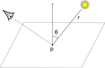
Because light in the real world does not perfectly reflect on surfaces but is scattered in different directions, there are several models that simulate this effect. Given the information about the location and normal of the intersection point and the location and properties of the light source, the specific material properties now define how the incident light is scattered. The so called bidirectional reflectance distribution function (Bidirectional reflectance distribution function (BRDF)) is often used to define these material properties. The light traveling towards the camera from that point has to be calculated by multiplying the incident light to the surface point with the corresponding BRDFof the surface. [PJH16]
A.2.2 Indirect Light Transport
With the use of rays [Whi80], also indirect reflections and transmissions can be simulated. Whitted’s method and path tracing solve the light transport equation with different accuracy, Whitted ray tracing uses simplified terms for the render equation. Path tracing solves the full equation by sending out many recursive rays per pixel (more on that later on). That means that at an intersection point another sub-ray will be cast to capture light that is incident to that point. These recursive steps make sure that the rendered image involves all the mutual reflections of the objects in the scene. However, Whitted’s method only accounts for recursive evaluation of perfect refraction and reflection. [PJH16]
A.2.3 LTE
As mentioned before, the light transport equation (Equation 2) is the fundamental equation that has to be solved in order to achieve correct results in synthesized images. It models all reflections at a point on a surface, including emission coming directly from the surface and the distribution of incoming light at that point. The fact that physical realism involves taking into account all objects in the scene that radiate or transmit light, the recursive (because of sub-paths) light transport equation has to be solved to achieve global illumination, however this makes the numerical evaluation difficult. [PJH16]
One important principle when using the light transport equation is energy conservation. In terms of points on surfaces, the outgoing radiance from that point must be equal to the emitted radiance minus the absorbed energy plus the incoming light that is scattered by the surface. This is derived from the general formula of the conservation of power (Equation 1.1 [PJH16]), where denotes the outgoing energy, the incoming energy, the emitted energy and the absorbed energy. [PJH16]
| (1) |
Eventually, the light transport equation for surfaces (Equation 1.2 [PJH16]) is as follows
| (2) |
where the first term describes the emitted light and the integral describes the incoming light that is scattered on that surface point.
A.2.4 Monte Carlo Integration solves the LTE
The following will give a brief overview on Monte Carlo Integration, which is fundamental for path tracing, since the underlying light transport equation cannot be computed analytically but only numerically using this method.
Monte Carlo Integration involves computations that approximate the integral of a given function by averaging randomly chosen samples. In the context of path tracing, this idea is applied by letting the algorithm go over one pixel several times, each time computing a random sample (light path). Statistically, averaging the different values from different runs will converge to the correct value. [PJH16]
In detail, Monte Carlo Integration aims at solving an arbitrary integral, in terms of 1D let it be . The expected value of the Monte Carlo Estimator (Equation 1.3 [PJH16]) estimates this integral.
| (3) |
where and the probability is uniformly distributed and denotes the number of random samples. In order to reduce variance from the integration, the underlying probability density function can be chosen heuristically to address this issue (Importance Sampling). This leads to the adapted estimator (Equation 1.4 [PJH16]).
| (4) |
The estimator can easily be used with higher dimensions, making it the only practical numerical method that converges high dimensional integrals independently from the dimensionality, that means the size of the dimension does not have impact on the performance of Monte Carlo Integration.
One negative aspect is that the error behaves inversely proportional to the amount of samples in a way that if the error should be halved, four times as many samples have to be evaluated. Graphically, approximation errors from the integration result in noisy pixels that are either too dark or too bright. [PJH16]
A.2.5 Advanced sampling methods
Path tracing was the first algorithm that solves the full light transport equation numerically. However, it can lead to partially very grainy images due to high variance in more complex lighting conditions [PJH16]. The following will give a brief overview on more advanced sampling techniques that are generally better than pure path tracing in terms of render quality and convergence time.
Next Event Estimation (NEE)
Next Event Estimation is a sampling technique that aims at reducing variance of Monte Carlo-sampling. Basically, NEEachieves this by searching for direct light sources at any path intersection. This can improve render performance and quality considerably when applied at every surface intersection of the path. [KNK+16]
Importance Sampling
Importance Sampling is a method for Monte Carlo Integration to reduce variance and convergence as well. The Monte Carlo Estimator from Equation 4 has the property that it converges faster if the samples are taken from a probability density function that is similar to in the integrand. Graphically, this means, the focus is on areas with high (relevant) values and therefore, calculations are faster and variance of the image decreases. [PJH16]
Bidirectional path tracer (BDPT)
BDPTis an extension to the common path tracing algorithm. It was developed independently by Lafortune and Willems [LW98] and Veach and Guibas [VG95]. It is called bidirectional because it does not only cast rays going out from the camera but also from the light sources. Basically, the algorithm knows all intersection points and attempts to connect pairs of them for each camera/light path. It then evaluates if a connection between pairs of intersections is not interrupted by another object. If this is the case, the corresponding path is added to the light estimation. BDPTgenerally speeds up the convergence of the light computation while also delivering less variance with fewer samples per pixel than path tracing. [PJH16]
BDPThas the advantage that the search for a relevant light source is easier unlike for Path tracing. A standard Path tracer shoots random rays into the scene trying to find light sources. Because it is very rare to find light sources with random rays in scenes with difficult light setups (for instance a light that is partially covered), resulting images often exhibit high variance. BDPTsimplifies this process and generally delivers images with less variance. The basic differences of light sampling between Path tracing and BDPTcan be seen in Figure 48.
Metropolis Light Transport, Path Space Metropolis Light Transport (MLT)
MLTwas first proposed by Veach and Guibas [VG97] in 1997. In contrast to the other methods, MLTis not based on the Monte Carlo method, specifically it creates samples that are statistically correlated. Basically, MLTsequentially shoots rays into the scene. Each subsequent ray is a mutation of the previous one using Markov chain techniques (the next sample state is dependent on the previous one). The main advantage of this method is that if a light path with high relevance is found, the following rays will search for further relevant paths in the neighborhood. The amount of searches in a region is therefore dependent on the relevance of the particular region in the scene. The basic principle of this method can be seen in Figure 48. This means that MLTis considerably good for scenes with difficult light situations like caustics where many light rays are located in small areas. However, MLTdoes have performance deficiencies when it comes to relatively simple and balanced light conditions. [PJH16]
There are several other sampling strategies that have different advantages and disadvantages, however this will not be covered in detail. Especially, BDPTand MLTwill be interesting related to the scene data set in the next chapter, because the light setups often require appropriate samplers to achieve good results in a reasonable time. Specifically, there will be scenes that have complex materials and light setups which can be easier or more difficult to sample depending on the chosen integrator.
The reason for this is illustrated by a simplified example showing a difficult scene setup in Figure 48. It shows the comparisons of the sampling strategies that were mentioned previously. The scenes described in this paper aim at challenging these strategies in order to understand their differences and examine potential shortcomings and problems. Difficulties in sampling will later be seen as variance in the renderings, depending on the sampling technique, the algorithms may give considerably different results.
