Renyi Entropy of Interacting Thermal Bosons in Large $N$ Approximation

Quantum entanglement and its various measures like entanglement entropies have become an important theoretical tool in the study of quantum many body systems. Starting from their domain of origin in the area of quantum information Eisert et al. 2010; Horodecki et al. 2009; Nielsen and Chuang 2002, where entanglement is considered as a resource for quantum computation Jozsa and Linden 2003, these measures have played an important role in the study of systems relevant to a wide variety of fields, from condensed matter theory to quantum gravity Ryu and Takayanagi 2006.

In condensed matter systems, entanglement entropy has been used to detect phase transitions Vidal et al. 2003; Orús 2008; Zhou et al. 2006; Hastings et al. 2010; Singh et al. 2012 and classify non-trivial topology of ground state of quantum systems  Jiang et al. 2012; Kitaev and Preskill 2006; Grover et al. 2011; Levin and Wen 2006. Entanglement entropy Kaufman et al. 2016 and entanglement spread Maldacena et al. 2016; Lezama and Luitz 2019 has been widely used to understand thermalization of complex many body systems. It has also been used to study many body localization Abanin et al. 2019; Alet and Laflorencie 2018; Samanta et al. 2020, where strongly disordered interacting quantum systems do not thermalize at long times. Entanglement entropy of many body system has recently been measured in experiments with ultracold atomic systems Islam et al. 2015.

While there is a large body of literature about entanglement entropy of Fermionic Swingle 2012; Peschel 2003 and spin systems Calabrese and Cardy 2005, relatively less attention has been paid to microscopic calculations of entanglement entropy of interacting Bosons. This is mainly due to the fact that the larger Hilbert space for Bosons do not allow numerical evaluation of entanglement entropy, unless the system is in the Tonk’s gas limit Alba and Calabrese 2017; Collura et al. 2013 in one dimension, or deep in the Mott insulator regime Farias and de Oliveira 2010; Ghosh et al. 2020, where the Hilbert space dimension can be manageable. The analytical approach comes from field theoretic considerations, where one either uses a replica based construction with a complicated manifold Casini and Huerta 2009, or takes advantage of simplifications from conformal field theories (CFT) if one is interested in a critical point Calabrese and Cardy 2009; Metlitski et al. 2009. While the CFT based approaches are most effective in one spatial dimensions, recent work has extended these considerations to more than one dimensions Whitsitt et al. 2017 for critical Bosons.

In a recent work Chakraborty and Sensarma we have developed a new field theoretic method, to calculate the Renyi entanglement entropy for a generic (interacting) open or closed many body Bosonic system undergoing arbitrary non-equilibrium dynamics Chakraborty et al. 2019. This method calculates the Wigner characteristic function Cahill and Glauber 1969 of a density matrix as the Schwinger-Keldysh (SK) partition function Kamenev and Levchenko 2009 of the system in the presence of sources turned on only at the time of measurement. For reduced density matrix of a subsystem, the sources need to be turned on only for degrees of freedom residing in the subsystem. The key new development is that unlike the well known replica based field theoretic approach to calculating entangelement entropy Casini and Huerta 2009, here one does not need to use complicated manifolds and can work with the standard field theory and its correlation functions. As a result, one is not restricted to particular geometries for the subsystem.

In this paper, we use this technique to calculate Renyi entanglement entropy of a thermal system of lattice Bosons at a fixed density, interacting with a local Hubbard repulsion. We consider $N$ species of Bosons and a ${\cal U}(N)$ symmetric interaction between the species Moshe and Zinn-Justin 2003. We show that in the large $N$ limit, the Renyi entropy of a subsystem is composed of two terms: (a) The Renyi entropy of an effective non-interacting system which has an additional spatially varying potential and (b) The difference in re-scaled thermal free energy between this effective system and the original translation invariant system within mean field approximation. This spatially dependent effective potential occurs due to the presence of the interactions between the Bosons and has no analogy in the case of non-interacting Bosons. Developing a systematic large $N$ expansion for the Renyi entropy of the interacting theory and interpreting it in terms of an effective non-interacting system with a self consistent spatially dependent potential is the key new result of this paper.

We divide a system of Bosons into two mutually exclusive sub-systems $A$ and $B$. We use field theoretic methods for calculating Wigner functions to construct a functional integral for the 2nd Renyi entropy of the subsystem $A$. We use saddle point approximation in the large $N$ limit to derive a self-consistent equation for the effective potential imposed by inter-particle interactions between the Bosons. We solve this equations numerically for a one dimensional chain and a two dimensional square lattice with nearest neighbour hopping and hence calculate the Renyi entropy of these systems. For the effective potential profile, we find (i) the potential profile takes the form of a step potential, which is flat in the bulk of the subsystem $A$ and the subsystem $B$ with different values and varies sharply across the entanglement cut (ii) The potential in the subsystem $B$ is just the thermal Hartree shift of the original system. (iii) The potential barrier $\Delta V$ increases with temperature and saturates at large temperatures. The effect of interactions on the entanglement entropy is controlled by $\Delta V/T$, which shows a peak at a characteristic temperature. (iv) The potential profile varies near the boundary of the subsystem $A$ on a lengthscale given by the density-density correlation length of the original thermal system. This variation would become important near a phase transition where the correlation length diverges.

Focussing on the Renyi entropy, we find that the entropy scales linearly with the size of the subsystem (as is expected for a thermal system), which allows us to define an entanglement entropy density of the subsystem. The entropy density increases monotonically with temperature and saturates to its non interacting value at high temperatures. The high and low temperature values are governed by the density of the system. The effects of the interaction parameter is largest at an intermediate temperature scale where the ratio of the potential barrier to the temperature is largest. We also define an excess entropy density due to tracing, which measures the additional entropy per site of the subsystem relative to the entropy per site of the thermal density matrix of the whole system. This excess entropy, which indicates the additional randomness generated by tracing over the subsystem $B$, monotonically decreases with temperature and goes to zero at large temperatures. We find these trends in both one dimensional and two dimensional systems with quantitative differences. We would like to note that a microscopic calculation of Renyi entropy in more than one dimension is less explored in the literature and our field theory formalism, which is agnostic about the dimensionality, is a new step in this direction.

We will now present a roadmap for navigating the paper. In Section  II, we review the well known relations between the Wigner characteristic function (WCF) of a density matrix and the second Renyi entropy of a subsystem. In Section III, we show that the WCF of a reduced density matrix of a thermal system can be written as a partition function with a specific set of sources within an imaginary time field theory. We work out the case of a system of non-interacting Bosons as an example in this section. In Section IV, we define the ${\cal U}(N)$ symmetric interacting model of $N$ species of Bosons and review its equilibrium field theory in the large $N$ limit. In Section 32, we focus on calculating the Renyi entropy of the ${\cal U}(N)$ symmetric model in the large $N$ limit. The key results and the interpretation in terms of an effective potential is developed in this section. In Section VI, we apply this formalism to study a one dimensional Bose gas, while in Section VII, we look at the case of a two dimensional Bose gas. We conclude in Section VIII with a summary and possible future directions to extend this formalism.

The Wigner function of a density matrix Wigner 1932 is the closest equivalent to a phase space distribution function for a quantum system. For a many body bosonic system, it is useful to define the Wigner Characteristics function (WCF), $\chi_{W}$ of the density matrix $\hat{\rho}$ Cahill and Glauber 1969,

$\displaystyle\chi_{W}(\{\gamma_{r}\})$

$\displaystyle=$

$\displaystyle\textrm{Tr}\left[\hat{\rho}\hat{D}(\{\gamma_{r}\})\right]=Tr\left[\hat{\rho}~e^{\sum\limits_{r}\gamma_{r}c^{\dagger}_{r}-\gamma^{\ast}_{r}c_{r}}\right],$

(1)

where $c^{\dagger}_{r}$ is the Bosonic creation operator for the spatial coordinate $r$, and $\hat{D}$ is the displacement operator which creates coherent states by acting on the ground state. Note that one can use any complete single particle basis to define the Wigner characteristics; we choose the position basis since it is the natural choice for calculation of entanglement entropies. The Wigner function is then defined by

$\displaystyle W(\{\alpha_{r}\})$

$\displaystyle=$

$\displaystyle\left[\int\prod_{r}\frac{d^{2}\gamma_{r}}{\pi^{\Omega}}e^{\sum\limits_{r}\gamma^{\ast}_{r}\alpha_{r}-\gamma_{r}\alpha^{\ast}_{r}}\chi_{W}(\{\gamma_{r}\})\right],$

(2)

where we consider a system with $\Omega$ lattice sites. One can follow the same procedure, with the density matrix replaced by the operator $\hat{O}$, to obtain the Weyl symbol of the operator

	$\displaystyle\chi_{O}(\{\gamma_{r}\})$	$\displaystyle=$	$\displaystyle\textrm{Tr}\left[\hat{O}\hat{D}(\{\gamma_{r}\})\right]$		(3)
	$\displaystyle W_{O}(\{\alpha_{r}\})$	$\displaystyle=$	$\displaystyle\left[\int\prod_{r}\frac{d^{2}\gamma_{r}}{\pi^{\Omega}}e^{\sum\limits_{r}\gamma^{\ast}_{r}\alpha_{r}-\gamma_{r}\alpha^{\ast}_{r}}\chi_{O}(\{\gamma_{r}\})\right].$

The expectation of the operator $\hat{O}$ is then given by the phase space integral

	$\displaystyle\langle\hat{O}\rangle$	$\displaystyle=$	$\displaystyle\textrm{Tr}~\hat{\rho}\hat{O}=\left[\int\prod_{r}\frac{d^{2}\alpha_{r}}{\pi^{\Omega}}W(\{\alpha_{r}\})W_{O}(\{\alpha_{r}\})\right]$		(4)
		$\displaystyle=$	$\displaystyle\left[\int\prod_{r}\frac{d^{2}\gamma_{r}}{\pi^{\Omega}}\chi_{W}(\{\gamma_{r}\})\chi_{O}(\{-\gamma_{r}\})\right]$

To calculate entanglement measures in a system, one considers a subsystem $A$ consisting of $\Omega_{A}$ sites. The reduced density matrix of the sub-system $A$, i.e. $\hat{\rho}_{A}(t)=Tr_{B}\hat{\rho}(t)$ is obtained by integrating out the degrees of freedom residing outside $A$ (i.e. in $B=A^{c}$ ). The second Renyi entropy of the subsystem $A$ is then given by

$$S^{(2)}=-\ln\textrm{Tr}~\hat{\rho}_{A}^{2}.$$

(5)

The Wigner characteristic function of the reduced density matrix can be obtained from the full density matrix in the following way,

$\displaystyle\chi^{A}_{W}(\{\gamma_{j}\})$

$\displaystyle=$

$\displaystyle\textrm{Tr}\left[\hat{\rho}\hat{D}(\{\gamma_{j}\})\right]=\textrm{Tr}\left[\hat{\rho}~e^{\sum\limits_{j}\gamma_{j}c^{\dagger}_{j}-\gamma^{\ast}_{j}c_{j}}\right],$

(6)

where the lattice index $j$ runs only over the $\Omega_{A}$ sites in the subsystem $A$, whereas the trace is over all degrees of freedom. The trace over the degrees of freedom in $B$ creates the reduced density matrix, while the displacement operator with support only in $A$ leads to the Wigner characteristic function of the reduced density matrix. Thus the WCF of the reduced density matrix is obtained from Eq. 1 by restricting the support of the displacement operator to the Hilbert space of the subsystem $A$. For the sake of simplicity and clarity of the notation, throughout this paper, we denote the lattice sites belonging to the sub-system, $A$ by the indices $j,j^{\prime}$ etc, i.e. $j,j^{\prime}\in A$ can run only over the $\Omega_{A}$ lattice sites, whereas we will use $r,r^{\prime}$ (or $x,y$) to indicate co-ordinates that run over the full system with $\Omega$ sites.

Finally, using Eq. 5 together with Eq. 4, we can write the second Renyi entropy of the subsystem in terms of the WCF of the reduced density matrix as

$$S^{(2)}=-\ln\left[\int\prod_{j\in A}\frac{d^{2}\gamma_{j}}{\pi^{\Omega_{A}}}|\chi^{A}_{W}(\{\gamma_{j}\},t)|^{2}\right].$$

(7)

We note that these results are quite general and are applicable to both non-interacting and interacting systems in and out of thermal equilibrium. In Ref. Chakraborty and Sensarma, a general Keldysh theory based formalism for calculating Renyi entropies of systems out of equilibrium has been formulated. However, in this paper, we focus on Renyi entropy of systems in thermal equilibrium and provide a detailed blueprint for calculating it within a field theory formalism. In the next section, we relate the Wigner characteristic of the reduced density matrix of a thermal system to a partition function with appropriate source configurations and apply it to a system of non-interacting Bosons.

For a system in thermal equilibrium, the density matrix in the grand canonical ensemble is given by $\hat{\rho}=\frac{1}{Z}e^{-\beta(\hat{H}-\mu\hat{N})}$, where $\hat{H}$ is the Hamiltonian of the system, $\beta=1/T$ is the inverse temperature, $\hat{N}$ is the total number operator and $\mu$ is the chemical potential. The partition function is given by $Z=\textrm{Tr}~e^{-\beta(\hat{H}-\mu\hat{N})}$, which ensures $\textrm{Tr}~\hat{\rho}=1$. The partition function can be expanded in a standard functional integral

	$\displaystyle Z$	$\displaystyle=$	$\displaystyle\int D[\phi]e^{-{\cal A}(\phi^{\ast}_{r},\phi_{r})},$		(8)
	$\displaystyle{\cal A}(\phi^{\ast}_{r},\phi_{r})$	$\displaystyle=$	$\displaystyle\!\!\!\int_{0}^{\beta}\!\!d\tau\!\!~\sum_{r}\!\phi^{\ast}_{r}(\tau)(\partial_{\tau}-\mu)\phi_{r}(\tau)\!+\!H[\phi^{\ast}_{r}(\tau),\phi_{r}(\tau)]$

where ${\cal A}$ is imaginary time action and $\hat{H}[c^{\dagger}_{r},c_{r}]$ is the normal ordered Hamiltonian of the system, and $\phi_{r}(\tau)$ are the Bosonic fields.

The WCF of the reduced density matrix of the subsystem $A$ is given by

			$\displaystyle\chi_{W}^{A}(\{\gamma_{j}\})=\frac{1}{Z}\textrm{Tr}~\left[e^{-\beta(\hat{H}-\mu\hat{N})}\times e^{\sum_{j}\gamma_{j}c^{\dagger}_{j}-\gamma^{\ast}_{j}c_{j}}\right]$		(9)
		$\displaystyle=$	$\displaystyle\frac{1}{Z}\textrm{Tr}~\left[e^{-(\beta-\beta_{0})(\hat{H}-\mu\hat{N})}\times\hat{D}(\{\gamma_{j}\})e^{-\beta_{0}(\hat{H}-\mu\hat{N})}\right]$

where $\beta_{0}$ is an arbitrary number between $0$ and $\beta$, and we have used the cyclic properties of the trace to write the last line. The numerator can be expanded in a functional integral

$\displaystyle\chi_{W}^{A}(\{\gamma_{j}\})$

$\displaystyle=$

$\displaystyle\frac{1}{Z}\int D[\phi]~e^{-\mathcal{A}[\phi,\phi^{*}]-\left(\sum\limits_{j}\gamma^{*}_{j}\phi_{j}(\beta_{0})-h.c.\right)}.~~$

(10)

The insertion of the displacement operator at the imaginary time $\tau_{0}=\beta_{0}$ is equivalent to turning on a source ¹¹ 1 Note that we have chosen here a slightly non-standard definition of partition function with linear sources compared to that in the standard thermal field theory, $Z[J_{j}(\tau)]=\int D[\phi]exp[-\mathcal{A}(\phi,\phi^{*})+\mathbf{i}\{\int_{0}^{\beta}J^{*}_{j}(\tau)\phi_{j}(\tau)+J_{j}(\tau)\phi^{*}_{j}(\tau)\}]$. This definition together with the choice $J_{j}(\tau)=-\mathbf{i}\gamma_{j}\delta(\tau-\beta_{0})$ takes care of the relative negative sign in $\hat{D}=exp[\sum_{j}\gamma_{j}a^{\dagger}_{j}-\gamma^{\ast}_{j}a_{j}]$. $-\mathbf{i}\gamma_{j}$ coupled to the field $\phi^{\ast}_{j}(\beta_{0})$ and $\mathbf{i}\gamma^{\ast}_{j}$ coupled to $\phi_{j}(\beta_{0})$. Note that the sources are turned on only for the fields in the subsystem $A$. They are turned on at the time $\beta_{0}$ and turned off immediately thereafter, creating a delta function profile in imaginary time. This suggests that the WCF $\chi_{W}^{A}(\{\gamma_{j}\})$ can be related to the equilibrium partition function Altland and Simons 2010 $Z$ in presence of linear delta function sources, $J_{j}(\tau)$, turned on only at $\tau=\beta_{0}$ for the modes $j\in A$, i.e.

$$\chi_{W}^{A}(\{\gamma_{j}\})=\frac{1}{Z}Z[J_{j}(\tau)=-\mathbf{i}\gamma_{j}\delta(\tau-\beta_{0})],~\forall j\in A.$$

(11)

where the denominator is calculated without any additional sources. This identification matches earlier results presented in Ref.Chakraborty and Sensarma, and can be considered as a special case of that more general result defined on real time Keldysh contours. Finally we note that the choice of $\beta_{0}$ is completely arbitrary and hence $\chi_{W}^{A}(\{\gamma_{j}\})$ is independent of the value of the imaginary time when the source is turned on. This will play a very important role when we consider an interacting model of Bosons in the next section.

We first apply this technique of calculating WCF and Renyi entropy of Bosonic systems to the simplest case of a generic non-interacting system of Bosons, with Hamiltonian, $H_{0}=\sum_{p}\epsilon_{p}c^{\dagger}_{p}c_{p}$ (See Ref. Drut and Porter 2017 for an alternate approach). We assume that the single-particle eigenstate $p$ has a wavefunction $\psi_{p}(r)$. We consider Bosons with density $\rho=(1/\Omega)\sum_{p}n_{B}(\epsilon_{p}-\mu,T)$, where $n_{B}(e,T)=1/[exp(e/T)-1]$, is the Bose distribution function and the chemical potential $\mu(T)$ is tuned to obtain the correct density at all temperatures. In this case, the action ${\cal A}$ is quadratic and we get

$\displaystyle\mathcal{A}[\phi,\phi^{*}]$

$\displaystyle=$

$\displaystyle\int\limits_{0}^{\beta}\int\limits_{0}^{\beta}d\tau d\tau^{\prime}\sum\limits_{r,r^{\prime}}\phi^{\ast}_{r}(\tau)G_{0}^{-1}(r,\tau;r^{\prime},\tau^{\prime})\phi_{r}(\tau^{\prime}).$

Here, $G_{0}^{-1}(r,\tau;r^{\prime},\tau^{\prime})$ is the imaginary time inverse Green’s function of the non-interacting system. Performing the Gaussian integration over the fields $\phi_{r}(\tau)$ in Eq.10, we obtain

$$\chi_{W}^{A}(\{\gamma_{j}\})=e^{-\sum\limits_{j,j^{\prime}}\gamma^{*}_{j}M^{A}(j,j^{\prime})\gamma_{j^{\prime}}},$$

(12)

where, $M^{A}(j,j^{\prime})=G_{0}(j,\beta_{0};j^{\prime},\beta_{0})$ is a $\Omega_{A}\times\Omega_{A}$ matrix. We note that one should be careful in taking the equal time limit $\tau=\tau^{\prime}=\beta_{0}$ in $\hat{M}^{A}$ from the time ordered Green’s function, $G_{0}(j,j^{\prime};\tau-\tau^{\prime})$, symmetrically along the imaginary time axis; i.e.

	$\displaystyle M^{A}(j,j^{\prime})$	$\displaystyle=$	$\displaystyle\frac{1}{2}\lim_{\eta\rightarrow 0^{+}}\Big[G_{0}(j,\beta_{0};j^{\prime},\beta_{0}+\eta)$		(13)
			$\displaystyle~~~~~~~~~~~~+G_{0}(j,\beta_{0};j^{\prime},\beta_{0}-\eta)\Big].$

The symmetric limit is due to the fact that the Wigner function is related to a symmetric rather than a (anti) normal ordering of $c$ and $c^{\dagger}$ operators. This limit also matches with the more general answer derived in Ref. Chakraborty and Sensarma using Keldysh field theory. Note that in this case the answer is independent of the choice of $\beta_{0}$, as we had predicted before on very general grounds. The system is still time-translation invariant along the imaginary time axis, $\tau$ and we can obtain the imaginary time Green’s functions by the standard Matsubara summation techniqueAltland and Simons 2010. This yields,

$$M^{A}(j,j^{\prime})=\frac{1}{2}\sum\limits_{p}\psi_{p}(j)\psi^{*}_{p}(j^{\prime})\left[1+2n_{B}(\epsilon_{p}-\mu,T)\right],$$

(14)

We now obtain $S^{(2)}$ by performing the Gaussian integration over the $\gamma_{j}$ variables in Eq. 7,

$$S^{(2)}=Tr_{A}\ln\left(2\hat{M}^{A}\right).$$

(15)

The entanglement entropy scales linearly with the subsystem size $\Omega_{A}$, as expected for a thermal density matrix. The above expression is further simplified if we calculate the Renyi entropy of the full system i.e. $j$ runs over all the lattice sites. In this case, $\hat{M}^{A}$ is a $\Omega\times\Omega$ matrix with eigenvalues, $m_{p}=[1+2n_{B}(\epsilon_{p}-\mu,T)]/2$. Substituting this in Eq. 15, we get

$$S^{(2)}=\sum\limits_{p}\log\left[\coth\left(\frac{\epsilon_{p}-\mu}{2T}\right)\right].$$

(16)

The above example of a simple case of non-interacting Bosonic systems gives a consistency check of the new field theoretic method proposed to calculate $S^{(2)}$ Drut and Porter 2017. In the subsequent sections, we will use this technique to calculate Renyi entropy of a reduced density matrix in presence of inter-particle interactions in the system.

In the previous section, we have obtained exact expressions for entanglement entropy of a subsystem of non-interacting Bosons which are in thermal equilibrium. Our aim is to extend this formalism to the case of interacting Bosons using a large $N$ formulation. To this end, we consider a Bose Hubbard model with $N$ species of Bosons. The Bosons hop between nearest-neighbour sites on a lattice and interact with local repulsive inter-species interaction given by,

$$H=-t\sum\limits_{\langle rr^{\prime}\rangle}\sum\limits_{a=1}^{N}c^{\dagger(a)}_{r}c^{(a)}_{r^{\prime}}+\frac{U}{2N}\sum\limits_{r}\sum_{a,b=1}^{N}c^{\dagger(a)}_{r}c^{\dagger(b)}_{r}c^{(a)}_{r}c^{(b)}_{r}$$

(17)

where $\langle r,r^{\prime}\rangle$ denote the nearest-neighbour lattice sites, $a,b$ are species indices which run from $1$ to $N$, $t$ is the hopping matrix element and $U$ is the scale of the local repulsion. We note that the scaling of the interaction, $U/N$, ensures that the energy of the system is extensive in the number of species $N$. It can be easily seen that this Hamiltonian is invariant under a global unitary rotation between the species, $c^{(a)}_{r}\rightarrow\tilde{c}^{(a)}_{r}=\mathcal{U}_{ab}c^{(b)}_{r}$, where $\mathcal{U}$ is an arbitrary $N\times N$ unitary matrix. We would study this $\mathcal{U}(N)$ symmetric model in the limit of large $N$.

Although our final aim is to calculate entanglement entropy of subsystems in this model, in this section, we will focus on the thermodynamics of the model. We will now calculate the partition function and hence free energy of this interacting Bosonic system in thermal equilibrium, using a large $N$ approximation Moshe and Zinn-Justin 2003. As we will find in the next section, this will form a part of the calculation of Renyi entropy of the subsystems. This will also allow us to discuss the large $N$ approximation and resulting saddle points in a known and simple example Moshe and Zinn-Justin 2003, while setting up notation for the large $N$ calculation of entanglement entropy, which we will take up in the next section.

For the standard thermal field theory, the action $\mathcal{A}$ of this $\mathcal{U}(N)$ symmetric model is given by

$\displaystyle\mathcal{A}[\phi,\phi^{*}]\!$

$\displaystyle=$

$\displaystyle\!\sum_{a=1}^{N}\!\int_{0}^{\beta}\!\!\!d\tau\!\sum\limits_{r}\phi^{*(a)}_{r}(\tau)\![\partial_{\tau}-\mu]\phi^{(a)}_{r}(\tau)\!-\!t\!\sum\limits_{\langle rr^{\prime}\rangle}\phi^{*(a)}_{r}(\tau)\phi^{(a)}_{r^{\prime}}(\tau)\!+\!\frac{U}{2N}\!\sum_{a,b=1}^{N}\!\int_{0}^{\beta}\!\!\!d\tau\!\sum\limits_{r}\!\phi^{*(a)}_{r}(\tau)\phi^{*(b)}_{r}(\tau)\phi^{(a)}_{r}(\tau)\phi^{(b)}_{r}(\tau).~~~~~$

(18)

Here, $\mu=\mu(T)$ is a chemical potential which ensures the correct number density per species $\rho$ in the system. We will vary $\mu$ so that $\rho$ is kept fixed at all temperatures. To calculate the partition function of this system in the large $N$ limit, we perform the standard Hubbard Stratonovich (HS) transformation on the quartic interaction term by introducing the auxiliary fields, $\lambda_{r}(\tau)$, which couples to the bi-linears of the fields, $\sum_{a=1}^{N}\phi^{*(a)}_{r}(\tau)\phi^{(a)}_{r}(\tau)$. Then the partition function reduces to

$\displaystyle Z$

$\displaystyle=$

$\displaystyle\int D[\phi]D[\lambda]~exp\left[-\frac{N}{2U}\int d\tau\sum\limits_{r}\lambda_{r}^{2}(\tau)-\int\limits_{0}^{\beta}\int\limits_{0}^{\beta}d\tau d\tau^{\prime}\sum\limits_{r,r^{\prime}}\sum\limits_{a=1}^{N}\phi^{*(a)}_{r}(\tau)\left[G^{-1}_{\lambda}(r,\tau;r^{\prime}\tau^{\prime})\right]\phi^{*(a)}_{r^{\prime}}(\tau^{\prime})\right],$

(19)

where the inverse propagator

$$G^{-1}_{\lambda}(r,\tau;r^{\prime}\tau^{\prime})=G_{0}^{-1}(r,\tau;r^{\prime},\tau^{\prime})-\mathbf{i}\lambda_{r}(\tau)\delta(\tau-\tau^{\prime})\delta_{rr^{\prime}}.$$

(20)

Here the non-interacting inverse propagator $G_{0}^{-1}(r,\tau;r^{\prime},\tau^{\prime})=\delta(\tau-\tau^{\prime})\left[(\partial_{\tau}-\mu)\delta_{rr^{\prime}}-t\delta_{\langle rr^{\prime}\rangle}\right]$. The $\phi$ integrations in Eq. 19 can be performed exactly to obtain,

$\displaystyle Z$

$\displaystyle=$

$\displaystyle\int D[\lambda]~e^{-N~Tr\ln\left[\hat{G}^{-1}_{\lambda}\right]-\frac{N}{2U}\int_{0}^{\beta}d\tau\sum\limits_{r}\lambda_{r}^{2}(\tau)},$

(21)

Note that each term in the exponent of Eq. 21 is multiplied by $N$. Now if we take the limit, $N\rightarrow\infty$, we can evaluate the integral over $\lambda$ in Eq. 21 in the saddle point approximation. Choosing a static uniform saddle point solution $-\mathbf{i}\lambda_{r}(\tau)=\lambda_{th}$ , the saddle point equation can be written as

$$\lambda_{th}=\frac{U}{\Omega}\sum\limits_{k}n_{B}(\epsilon_{k}+\lambda_{th}-\mu,T),$$

(22)

where the dispersion for a hypercubic lattice in $d$ dimension is $\epsilon_{k}=-2t\sum_{i=1}^{d}\cos k_{i}$. In addition, we have to solve the number equation

$$\rho=\frac{1}{\Omega}\sum\limits_{k}n_{B}(\epsilon_{k}+\lambda_{th}-\mu,T).$$

(23)

It is then easy to show that the saddle point solution is $\lambda_{th}=U\rho$, which is the standard Hartree energy shift in the system.

Substituting this saddle point value of the auxiliary variable $\lambda_{th}$ in Eq. 21 we obtain the free energy within the large $N$ approximation,

$$F=\frac{N\Omega}{2}U\rho^{2}-NT\sum\limits_{k}\ln\left[1-e^{-\frac{\epsilon_{k}+\lambda_{th}-\mu}{T}}\right]$$

(24)

We note that for stability of the system, the effective chemical potential $\mu-\lambda_{th}$ must be lower than the bottom of the band dispersion, $-2td$. Bose Einstein condensation in this system occurs when $\mu-\lambda_{th}$ reaches the bottom of the band. In one dimension, this happens only at $T=0$. In two dimensions the large $N$ mean field theory for Schrodinger Bosons precludes the possibility of Bose Einstein condensation due to a weak logarithmic infrared divergence in the number equation. The physics of vortex binding and unbinding, which is missing from this description, leads to a BKT transition in this case. In three dimension, the large $N$ theory predicts a finite temperature phase transition. In this paper we will confine ourselves to the “high temperature” or non-condensed phases of the Bosons. The case of the ordered phase will be taken up in a future work.

In the next section, we will modify the large $N$ procedure described above for calculating the Wigner characteristic and hence Renyi entropies of a subsystem of interacting thermal Bosons.

In this section, we will devise a large $N$ approximation to calculate the Renyi entropy of a subsystem of interacting Bosons. The standard large $N$ approximation for the thermal field theory of $\mathcal{U}(N)$ model has two parts: a Hubbard Stratanovich transformation with an auxiliary field coupled to a $\mathcal{U}(N)$ invariant bilinear of the fields, and a saddle point evaluation of the integrals over the auxiliary fields, justified by the $N\rightarrow\infty$ limit. Since the large $N$ approximation for the partition function has already been shown in the last section, here we focus on the partition function in presence of the sources, i.e. the WCF $\chi_{W}^{A}(\{\gamma_{j}\})$.

We will use the path integral representation of $\chi_{W}^{A}(\{\gamma_{j}\})$ shown in Eq. 10, with the action given by Eq. 18. Note that in this case each species of the Boson fields are coupled to sources. Following the steps in the previous section, we will first decouple the interaction terms in $\mathcal{A}$ by a HS transformation to get

	$\displaystyle\chi_{W}^{A}(\{\gamma_{j}\})$	$\displaystyle=$	$\displaystyle\frac{1}{Z}\int D[\lambda]D[\phi]~e^{\left[-\frac{N}{2U}\int d\tau\sum\limits_{r}\lambda_{r}^{2}(\tau)-\int\int d\tau d\tau^{\prime}\sum\limits_{r,r^{\prime}}\sum\limits_{a=1}^{N}\phi^{*(a)}_{r}(\tau)\left[G^{-1}_{\lambda}(r,\tau;r^{\prime}\tau^{\prime})\right]\phi^{*(a)}_{r^{\prime}}(\tau^{\prime})\right]}$		(25)
			$\displaystyle~~~~~~~~~~~~~~~~~~~~~~~~~~~~~~~~~~~~~~~~~~~~\times e^{-\left(\sum\limits_{j}\sum\limits_{a=1}^{N}\gamma^{*(a)}_{j}\phi^{(a)}_{j}(\beta_{0})-h.c.\right)}.~~~$

where we would like to emphasize once again that $r,r^{\prime}$ runs over all lattice sites, while $j$ runs only over the subsystem $A$. The partition function $Z$ in the denominator has already been calculated in the previous section. The Gaussian functional integration over the fields $\phi_{r}(\tau)$ yields

$\displaystyle\chi_{W}^{A}(\{\gamma^{(a)}_{j}\})$

$\displaystyle=$

$\displaystyle\frac{1}{Z}\int D[\lambda]~e^{-N~Tr\ln\left[\hat{G}^{-1}_{\lambda}\right]-\frac{N}{2U}\int d\tau\sum\limits_{r}\lambda_{r}(\tau)^{2}-\sum\limits_{j,j^{\prime}}\sum\limits_{a=1}^{N}\gamma^{*(a)}_{j}M^{A}_{\lambda}(j,j^{\prime})\gamma^{(a)}_{j^{\prime}}},$

(26)

where, $\hat{G}^{-1}_{\lambda}$ is the interacting inverse propagator defined in Eq. 20. Once again, $M^{A}_{\lambda}(j,j^{\prime})=G_{\lambda}(j,\beta_{0};j^{\prime},\beta_{0})$, with the equal time limit taken symmetrically as defined in Eq. 13. In this case, it is useful to substitute $\chi_{W}^{A}$ from Eq. 26 in Eq. 7 and perform the Gaussian integration over the source variables, $\gamma^{(a)}_{j}$. We then obtain the Renyi entanglement entropy, $S^{(2)}$ from,

	$\displaystyle e^{-S^{(2)}}=\int\prod_{a,j}\frac{d^{2}\gamma^{(a)}_{j}}{\pi^{N}}|\chi^{A}_{W}(\{\gamma^{(a)}_{j}\})|^{2}$	$\displaystyle=$	$\displaystyle\frac{1}{Z^{2}}\int D[\lambda]\int D[\nu]e^{-N~\left\{Tr\ln\left[\hat{G}^{-1}_{\lambda}\right]+Tr\ln\left[\hat{G}^{-1}_{\nu}\right]\right\}}$		(27)
			$\displaystyle~~~\times~e^{-\frac{N}{2U}\int d\tau\sum\limits_{r}\left[\{\lambda_{r}(\tau)\}^{2}+\{\nu_{r}(\tau)\}^{2}\right]-N~Tr_{A}\left[\ln\{\hat{M}^{A}_{\lambda}+\hat{M}^{A}_{\nu}\}\right]}.$

The exponent in the integral is multiplied by $N$, and in the limit of large $N$, we can evaluate the above integral over the two auxiliary fields using saddle point approximation. Note that the saddle point solutions will be different from that of the thermal field theory due to the extra term $\sim Tr_{A}\ln\{\hat{M}^{A}_{\lambda}+\hat{M}^{A}_{\nu}\}$, which comes from integrating over the source variables $\gamma^{(a)}_{j}$ of the WCF. This term only depends on the Green’s functions in the sub-system $A$. Symmetry indicates that the saddle point profiles $\lambda^{0}_{r}(\tau)=\nu^{0}_{r}(\tau)$. Considering the saddle point condition, we get

$$\frac{\lambda^{0}_{r}(\tau)}{U}=\mathbf{i}G_{\lambda^{0}}(r,\tau;r,\tau)-\frac{\mathbf{i}}{2}\sum\limits_{j,j^{\prime}}~\left[G_{\lambda^{0}}(r,\tau;j,\beta_{0}){M}_{\lambda^{0}}^{A(-1)}(j,j^{\prime})G_{\lambda^{0}}(j^{\prime},\beta_{0};r,\tau)\right].$$

(28)

The first term in Eq. 28 is the standard answer one gets for the thermodynamics of the system. This term is independent of $\tau$ as well as independent of $\beta_{0}$. The second term comes from integrating out the sources $\gamma^{(a)}_{j}$. This is an additional term that occurs when evaluating the Renyi entropy and depends explicitly on $\tau$ as well as on $\beta_{0}$. However, as we had mentioned before, the choice of $\beta_{0}$ is arbitrary and answers should not depend on this variable. Hence, we integrate over the variable $\beta_{0}$ from $0$ to $\beta$ and divide by $\beta$. This approximation allows us to consider a spatially varying, but (imaginary) time independent saddle point profile $\lambda^{0}_{r}$, given by

	$\displaystyle\frac{\lambda^{0}_{r}}{U}$	$\displaystyle=$	$\displaystyle\mathbf{i}G_{\lambda^{0}}(r,\tau;r,\tau)-\frac{\mathbf{i}}{2\beta}\int\limits_{0}^{\beta}d\beta_{0}\sum\limits_{j,j^{\prime}}~\left[G_{\lambda^{0}}(r,\tau;j,\beta_{0}){M}_{\lambda^{0}}^{-1}(j,j^{\prime})G_{\lambda^{0}}(j^{\prime},\beta_{0};r,\tau)\right]$		(29)
		$\displaystyle=$	$\displaystyle\mathbf{i}G_{\lambda^{0}}(r,r;0)-\frac{\mathbf{i}}{2\beta}\int\limits_{0}^{\beta}d\tau\sum\limits_{j,j^{\prime}}~\left[G_{\lambda^{0}}(r,j;-\tau){M}_{\lambda^{0}}^{A(-1)}(j,j^{\prime})G_{\lambda^{0}}(j^{\prime},r;\tau)\right].$

Note that we have restored the (imaginary) time translation invariance of the problem, and hence one can use Matsubara frequency sums to evaluate the integrals above. The saddle point is then equivalent to an effective non-interacting Hamiltonian with a spatially varying external potential $V(r)=-\mathbf{i}\lambda^{0}_{r}$, which has to be determined self consistently. If the eigenvalues and eigenfunctions of this effective single particle Hamiltonian

$$H_{eff}=H_{0}+V(r)-\mu,$$

(30)

are $E_{n}$ and $\psi_{n}(r)$ ($H_{0}$ is the non-interacting part of the original Hamiltonian given in Eq. 17), the self-consistency equation is given by

$\displaystyle\frac{V(r)}{U}$

$\displaystyle=$

$\displaystyle\sum\limits_{n}|\psi_{n}(r)|^{2}~n_{B}(E_{n},T)+T\sum\limits_{nn^{\prime}}\sum\limits_{j,j^{\prime}}\psi_{n}(r)\psi^{*}_{n}(j)\psi_{n^{\prime}}(j^{\prime})\psi^{*}_{n^{\prime}}(r)\frac{[n_{B}(E_{n},T)-n_{B}(E_{n^{\prime}},T)]}{E_{n}-E_{n^{\prime}}}M_{\lambda^{0}}^{A(-1)}(j,j^{\prime})$

(31)

Substituting this saddle point solution, $V(r)$ in Eq. 27, we obtain the Renyi entanglement entropy in the large $N$ limit,

	$\displaystyle{\cal S}^{(2)}=\frac{S^{(2)}}{N}$	$\displaystyle=$	$\displaystyle-\frac{\beta}{U}\sum\limits_{r}V^{2}(r)+2\sum\limits_{n}\ln\left[1-e^{-\beta E_{n}}\right]+\frac{\Omega\beta}{U}\lambda_{th}^{2}-2\sum\limits_{p}\ln\left[1-e^{-\beta(\epsilon_{p}+\lambda_{th}-\mu)}\right].$		(32)
		$\displaystyle+$	$\displaystyle Tr_{A}\ln\left[2\hat{M}^{A}_{V(r)}\right]$

We note that the leading order approximation to the entanglement entropy simply scales with the number of Boson components $N$, and hence it is useful to define the entropy per species of the Bosons. From the above formula we see that the entanglement entropy of the system in large $N$ approximation has two contributions: (a) the first line corresponds to the difference of the re-scaled thermodynamic free energy, $\beta F$ of two systems: the original translation invariant system that we are interested in, and the “effective” system with a spatially dependent potential $V(r)$, stemming from the entanglement cut in the system, which has to be self-consistently determined from Eq. 31 and (b) a second contribution (second line) related to the one-particle correlation function $M$ within the subsystem $A$. This correlation function is calculated for the system with the “effective” Hamiltonian. Note that in case of a non-interacting system, there is no effective potential, and hence we simply get the second line as the full answer. Our formalism thus generalizes the non-interacting answers to the case of interacting system within the large $N$ approximation.

In the next two sections, we will use this large $N$ solution to calculate the Renyi entropy of a $1$-d and $2$-d interacting Bose gas.

We consider a one dimensional chain of size $L$, where Bosons hop with a nearest neighbour tunneling amplitude $t$ and interact locally with a repulsive interaction scale $U$. Considering $N$ species of Bosons, the ${\cal U}(N)$ symmetric Hamiltonian is given by

$\displaystyle H\!=\!\!-t\!\sum\limits_{x}\!\sum\limits_{a=1}^{N}\!c^{\dagger(a)}_{x}c^{(a)}_{x+1}\!+\!h.c\!+\!\frac{U}{2N}\!\sum\limits_{x}\!\sum_{a,b=1}^{N}\!c^{\dagger(a)}_{x}c^{\dagger(b)}_{x}c^{(a)}_{x}c^{(b)}_{x},$

where $a,b$ indicate the species index of the Bosons. The Hamiltonian has periodic boundary conditions to ensure translational invariance. This leads to a dispersion $\epsilon_{p}=-2t\cos p$, where $p$ is the lattice momentum. We will set $t=1$ and the lattice-spacing $a=1$ to fix units of energy and length in all subsequent discussion in this paper. For 1D chain, the band energies vary between $-2$ and $+2$, giving a bandwidth of $4t=4$. We consider the system at a temperature $T$ with a fixed density $\rho$, while we allow the chemical potential $\mu$ to vary with temperature. This ensures the same number density at all temperatures. We are interested in the Renyi entropy of the reduced density matrix of a contiguous subsystem of size $L_{A}$. Note that due to the translation invariance of the original Hamiltonian, this subsystem can be placed anywhere in the system; we choose to place it in the left half of the system. In this section, we will work with $L=100$, unless otherwise mentioned.

For a lattice Boson system, the chemical potential lies below the bottom of the band at high temperatures. If the chemical potential reaches the bottom of the band, Bose Einstein condensation occurs in the system. It is well known that in $1$ dimension, the low energy divergence of the single-particle density of states $D(\epsilon)\sim\epsilon^{-1/2}$, together with the $\sim\epsilon^{-1}$ divergence of the Bose function, $n_{B}(\epsilon)=[e^{\beta\epsilon}-1]^{-1}$, prevents the formation of a BEC in the system. This remains true for the interacting system within the large $N$ approximation. Thus our formalism, which does not take into account possible Bose condensation, works at all temperatures for the $1$ dimensional system.

The first task in calculating the Renyi entropy of a subsystem is to obtain the self-consistent profile of the effective potential $V(x)$ from the saddle point equation Eq. 31. The self-consistent profile obtained for three different temperatures, $T=7.5$, $T=2.5$ and $T=1$ are plotted as a function of the lattice sites in Fig. 1(a). In this case, $U=0.5$ and $\rho=0.5$. From the figure, we see that the potential has a flat profile in the bulk of subsystem $A$ with a value $V_{A}$ and a similar flat profile with a different value $V_{B}$ in the bulk of subsystem $B$. It changes near the entanglement cut at $x=50$ and $x=0$ very rapidly over a scale of a few lattice spacings. This is depicted schematically in Fig. 1(b) as a step potential barrier with a height $\Delta V(T)=V_{B}(T)-V_{A}(T)$. Near the entanglement cut, we find that the potential in the subsystem $A$ drops near the edge before rising sharply in the $B$ subsystem. The lengthscale of variation on either side is almost equal to the correlation length $\xi(T)$, obtained from the exponential decay of the connected density-density correlation function in the thermal system. This is not surprising if we think of the entanglement cut as a localized source of disturbance. One would then expect the local density, and hence the effective potential, to adjust to this perturbation on a scale of $\xi(T)$. To see this clearly, we plot the potential profile at $T=0.1$ in Fig. 1(c), where the variation of the potential occurs on a measurable length scale of $\sim 9$. In the inset of Fig. 1(c), we plot $\xi(T)$ with the temperature of the system. We see that at $T=0.1$, $\xi(T)$ is also $\sim 9$. The key takeaway from this is that, while the entanglement calculation inevitably involves solving a translation non-invariant problem of the effective potential (even though the original system is translation invariant), one can get away with solving a much simpler problem of a step potential well in the subsystem $A$, as long as the correlation length $\xi(T)$ is much smaller than the subsystem size $L_{A}$. However, the value of the barrier needs to be solved self-consistently. This can in principle be used to calculate entanglement entropies in large systems in higher dimensions. We note that this potential barrier is imposed by the effect of the inter-particle interactions in the system and vanishes in the limit $U\rightarrow 0$.

The bulk value of the potential in the subsystem $B$, $V_{B}$ is independent of the temperature, as seen from Fig. 1(a). In fact, this value is simply the thermal value of the auxiliary field $\lambda_{th}=U\rho$. To see this, we plot $V_{B}$ for systems with different values of $U$ and $\rho$ as a function of $U\rho$ in Fig. 1(d), and obtain a straight line with unit slope. The potential barrier across the entanglement cut increases with temperature, saturating at very high temperatures. This is shown in Fig. 1(e) for three different set of parameters: $U=0.5,~\rho=0.5$ (blue solid line), $U=1,~\rho=0.5$ (purple dashed line) and $U=1,~\rho=1$ (green dashed-dotted line). The high temperature saturation value increases with density of the system as well as with the interaction in the system.

Since we are considering a thermal system with a potential barrier, the effects of this barrier, and hence of interaction in the system, on ${\cal S}^{(2)}$ will be controlled by the dimensionless parameter $\Delta V/T$. This is plotted in Fig. 1(f) as a function of temperature for three different set of parameters: systems with $U=0.5,~\rho=0.5$ (blue solid line), $U=1,~\rho=0.5$ (purple dashed line) and $U=1,~\rho=1$ (green dashed-dotted line). The dimensionless parameter peaks at a typical value of temperature $T_{\mathrm{max}}$ before going down as $\sim T^{-1}$ at large temperatures. $T_{\mathrm{max}}$ increases with increasing $U$ and $\rho$. We should expect the effects of interaction on ${\cal S}^{(2)}$ to be largest around $T_{\mathrm{max}}$ .

We now focus on the Renyi entanglement entropy of the subsystems of this interacting thermal system. The entanglement entropy scales linearly with the size of the subsystem, as expected for a thermal density matrix. To show this, in Fig 2(a), we plot the entanglement entropy of a subsystem with $L_{A}$ for a system of size $L=600$ and $U=0.5$, $\rho=0.5$ for two different temperatures, $T=3$ and $T=0.1$. This allows us to define an entanglement entropy density (entanglement entropy per site per species of the Bosons), $\mathfrak{s}^{(2)}$ and we will now focus on how this entanglement entropy density changes with temperature, density and interaction in the system. In Fig. 2(b), we plot the entanglement entropy density for a subsystem of size $L_{A}=50$ as a function of temperature. This is done for a system with $L=100$ and $U=1$ and two different values of density, $\rho=0.5$ and $\rho=1.0$. The entropy density increases with temperature and saturates at high temperatures. At large $T$, $\mathfrak{s}^{(2)}$ (triangles) closely agrees with the non-interacting answer ($=\log(\coth[|\mu|/2t])$) plotted by red solid line in the inset of Fig. 2(b) for $\rho=0.5$. This can be understood in the following way: the chemical potential $|\mu(T)|$ (solid line with squares) increases linearly with $T$ as shown in the inset of Fig. 2(b) and at large $T$, $\Delta V(T)$ imposed by the inter-particle interaction becomes negligible compared to $\mu(T)$. Hence, at large $T$ the effects of interaction becomes completely suppressed in $\mathfrak{s}^{(2)}$. This is expected since $\Delta V/T$ goes to $0$ in this limit, as seen from Fig. 1(e).

In order to understand the effect of interaction on entanglement entropy density, we consider $\Delta\mathfrak{s}^{(2)}=\mathfrak{s}^{(2)}(U)-\mathfrak{s}^{(2)}(0)$ , the difference between the entropy density of an interacting system and that of a non-interacting system at the same temperature and density. In Fig 2(c), we plot $\Delta\mathfrak{s}^{(2)}$ as a function of temperature for a system with $\rho=0.5$ for three different values of $U=0.5$, $U=1.5$ and $U=2.5$. We note that $\Delta\mathfrak{s}^{(2)}$ increases at low temperature and reaches a peak before going down at large temperatures. The large temperature decay $\sim T^{-1}$, reflecting similar decay in the dimensionless potential barrier $\Delta V/T$, shown in Fig. 1(e). In fact, the behaviour of $\Delta\mathfrak{s}^{(2)}$ is very similar to that of $\Delta V/T$ over the full temperature range considered here. The peak position and the peak value of $\Delta\mathfrak{s}^{(2)}$ increases with increasing $U/t$. In Fig 2(c), we have also shown the peak positions of $\Delta V/T$ with color coded arrows for the same parameters. This shows that the peak of $\Delta\mathfrak{s}^{(2)}$ closely tracks that of $\Delta V/T$.

Every density matrix of a quantum system (or subsystem) can be interpreted in terms of an ensemble of pure quantum states drawn with a particular classical probability distribution. If one diagonalizes the density matrix, the eigenstates are the pure quantum states in question and the eigenvalues are the corresponding probabilities. It is obvious that entropy measures defined on density matrices are actually entropy measures of the corresponding classical probabilities associated with the density matrix. For example, the Renyi entropy of a density matrix $S^{(2)}=-\ln\textrm{Tr}\hat{\rho}^{2}=-\ln\sum_{i}p_{i}^{2}$, where the eigenvalues $p_{i}$ correspond to the classical probability distribution.

For entanglement measures, when one constructs the reduced density matrix of a subsystem from a pure quantum state in the full system by tracing over degrees of freedom, the loss of the “quantum” information shows up as a classical probability distribution in the reduced description. Entanglement entropies are various entropy measures of this distribution and measures the classical randomness associated with the loss of the “quantum” information. However, when the state of the full system is described by a density matrix, as is the case for thermal systems at finite temperature, there is a classical randomness associated with the full system as well. In this case, we can define the additional randomness introduced by the loss of information (tracing), i.e. an entropy density of tracing by considering the difference between the entropy density of the subsystem, calculated from the reduced density matrix, and the entropy density of the full system, calculated from the full thermal density matrix, $\mathfrak{S}^{(2)}=\mathfrak{s}^{(2)}(L_{A})-\mathfrak{s}^{(2)}(L)$. This is a measure of the additional randomness introduced by tracing over the subsystem $B$. Note that since the number of degrees of freedom is different in the subsystem and the full system, it is important to divide the entropy by the size of the corresponding system before subtracting them.

In Fig 2(d), we plot the additional entropy density $\mathfrak{S}^{(2)}$ of a subsystem of size $L_{A}=50$ for a system with $L=100$, $U=1$ and $\rho=0.5$ as a function of temperature. We see that the additional entropy density is a monotonically decreasing function of temperature, going to $0$ at very large temperatures. At low temperatures, the full system is in a almost pure quantum state and the entropy density of the full system $\mathfrak{s}^{(2)}(L)$ is very small. Hence, a large entropy density is gained by tracing out the degrees of freedom. On the other hand at very high temperatures, the system behaves like a bunch of classical free particles and hence tracing does not lead to generation of any additional randomness in the system.

In the next section, we will extend this discussion to the case of a 2D interacting Bose gas.

In this section we extend our formalism to a $2$ dimensional system. We would like to note that a microscopic calculation of Renyi entropy in more than one dimension is less explored in the literature and our field theory formalism which is agnostic about the dimensionality of the system is a new step in this direction. We consider a Bose gas on a square lattice with nearest neighbour hopping $t$ and a local Hubbard repulsion $U$. Once again, we consider $N$ species of Bosons and a ${\cal U}(N)$ symmetric model given by

	$\displaystyle H$	$\displaystyle=$	$\displaystyle-t\sum\limits_{\langle rr^{\prime}\rangle}\sum\limits_{a=1}^{N}c^{\dagger(a)}_{r}c^{(a)}_{r^{\prime}}+h.c.$		(33)
		$\displaystyle+$	$\displaystyle\frac{U}{2N}\sum\limits_{r}\sum_{a,b=1}^{N}c^{\dagger(a)}_{r}c^{\dagger(b)}_{r}c^{(a)}_{r}c^{(b)}_{r}$

With a periodic boundary condition in both $x$ and $y$ direction, we can work in the lattice momentum basis with a dispersion $\epsilon_{p}=-2t(\cos p_{x}+\cos p_{y})$, resulting in a bandwidth of $8t$. The non-interacting system does not undergo a Bose Einstein condensation at any finite temperature due to an infrared logarithmic divergence in the number equation in $2$-d , in accordance with the Mermin-Wagner theorem Altland and Simons 2010. While the real system would show a Berezinskii Kosterlitz Thouless type transition at a finite temperature to a disordered phase from a phase with quasi-long range order due to proliferation of vortices, this is not captured within a large $N$ theory, which does not account for the vortex excitations.

We consider the large $N$ approximation to the Renyi entropy of a $L_{A}~\times~L_{A}$ subsystem located around the center of a $L~\times~L$ lattice. We will present data for $L=24$ and $L_{A}=12$ in this section, unless otherwise mentioned. We first consider the effective potential $V(x,y)$ for this system.

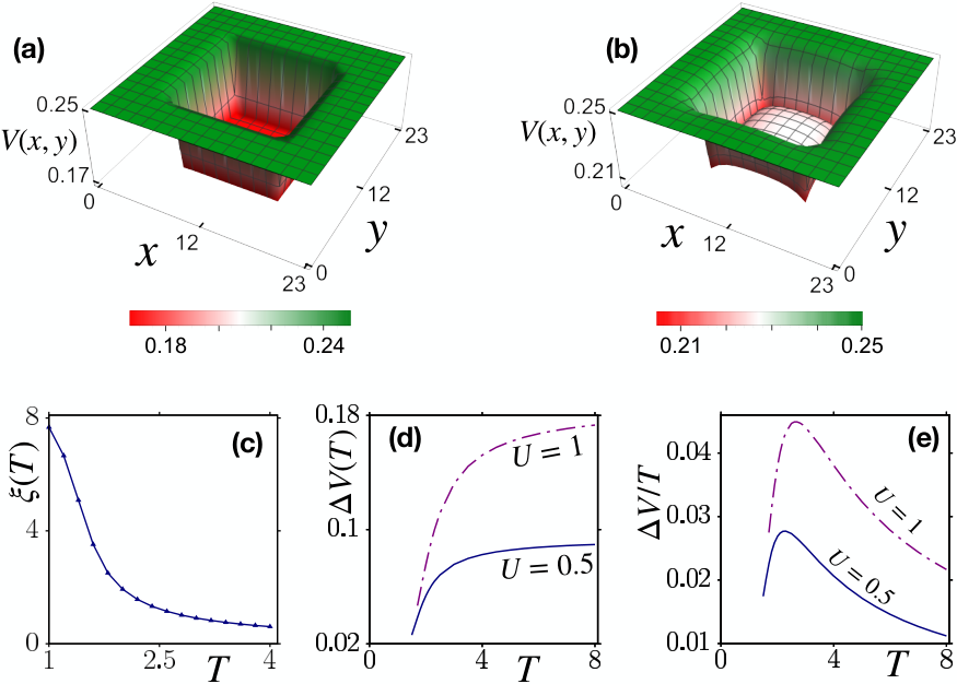
The effective potential profile for a system with density $\rho=0.5$ and interaction strength $U=0.5$ is shown in Fig. 3. Fig. 3 (a) plots the effective potential profile for a high temperature $T=4.0$. Similar to the one dimensional case, we find that $V(x,y)$ is almost constant in the subsystem $B$ and sticks to its thermal value $U\rho$. The potential forms an almost square well inside the subsystem $A$ with a constant value $V_{A}$. The potentials match up at the boundary separating the subsystem $A$ from the subsystem $B$ on a scale of the connected density-density correlation length. Fig. 3(b) plots the effective potential profile for the same system at a lower temperature of $T=1.5$. In this case, the profile varies around the entanglement cut on a larger lengthscale. In fact, for a subsystem size of $12\times 12$, the potential profile within the subsystem $A$ looks almost parabolic and leads to deep pockets at the corners of the entanglement cut. To understand this behaviour, we have plotted the thermal connected density-density correlation length $\xi(T)$ as a function of temperature in Fig. 3(c). We see that the correlation length is $\sim 5$ at $T=1.5$, and hence the subsystem size is already of the same scale as the correlation length at this temperature within our finite size calculation. This explains the large spatial variations of the effective potential profile in this case.