Construction of $bb\bar{u}\bar{d}$ tetraquark states on lattice
with NRQCD bottom and HISQ up/down quarks

For $bb\bar{u}\bar{d}$ mass calculation, we need nonperturbative tuning of both $m_{b}$ and $m_{u/d}$. With the help of equation (8), the tuning of $m_{b}$ has been carried out by calculating the spin average of $\Upsilon$ and $\eta_{b}$ kinetic masses and comparing the same with the spin average and suitably adjusted experimental $\Upsilon$ and $\eta_{b}$ masses as discussed in section II. The tuned bare $am_{b}$ quark masses for lattices used in this work are given in Table 2.

But the tuning of $am_{u/d}$ is rather tricky. It was found in protick that the $B$-meson tuned $am_{u/d}$ reproduces the mass of $\Sigma_{b}$ baryon but not that of $\Lambda_{b}$. Therefore, we tuned $am_{u/d}$ to two different values depending on the construction of the pairs $[ud]$ and $[bu]$ or $[bd]$. The motivation to do so followed from the observation that substantial mass difference exist among singly heavy baryons having same quark content and same $J^{P}$. For instance, the mass differences between the $J^{P}={1\over 2}^{+}$ pairs $(\Lambda_{b},\,\Sigma_{b}\,[bdu])$, $(\Lambda_{c},\,\Sigma_{c}\,[cdu])$, $(\Xi_{b},\,\Xi_{b}^{\prime}\,[bsu])$ and $(\Xi_{c},\,\Xi_{c}^{\prime}\,[csu])$ are in the range $110-190$ MeV. The $\Lambda_{b}$, $\Lambda_{c}$, $\Xi_{b}$ and $\Xi_{c}$ baryons are characterized by the spin of the $[l_{1}l_{2}]$ (where $l_{1,2}\in u,\,d,\,s$) light-light diquark $s_{l}=0$ while $\Sigma_{b}$, $\Sigma_{c}$, $\Xi_{b}^{\prime}$ and $\Xi_{c}^{\prime}$ by $s_{l}=1$. This differences in their wave functions alone cannot generate such mass differences bowler_54 but can at most account for a difference of about 30 MeV. The heavy hadron chiral perturbation theory calculations tiburzi; zachary for $\Lambda_{Q}$ and $\Sigma_{Q}$, where $Q\in b,c$, demonstrated that the mass differences get large correction of the order $\approx 150$ MeV. A correction of similar magnitude is anticipated in our NRQCD-HISQ heavy baryon / tetraquark systems, but the relevant $\chi$PT for which is yet to be available. To include such a correction in our calculations, we propose this unique method of tuning the $[\bar{u}\bar{d}]$ diquark system to $\Lambda_{b}$-baryon and $[b\bar{u}]$ to $B$-meson.

In the present paper, we try to understand this tuning scheme in more details with the help of relativised quark model mes_q_mod; bar_q_mod and Hartree-Fock calculation. The basic idea is that $am_{u/d}$ has to be tuned to two different values corresponding to two different constructions of the pairs $[\bar{u}\bar{d}]$ and $[b\bar{u}]$. In the operator $\mathcal{O}_{D}\equiv[bb][\bar{u}\bar{d}]$, the anti-diquark part formed with two light $u/d$ quarks is the same that appear in the baryonic operator $\Lambda_{b}\equiv(u^{T}C\gamma_{5}d)\,b$, and hence, we use experimental $\Lambda_{b}$ mass 5620 MeV to tune the bare $am_{u/d}$. For the operators $\mathcal{O}_{M_{1}/M_{2}}$, the diquark part is formed between heavy quark and light antiquark $[b\bar{u}]$ which is the same as in the $B$-meson $(\bar{b}\gamma_{(5,k)}u)$ or $\Sigma_{b}\equiv(Q^{T}C\gamma_{5}\,u)\,u$. In such case we tend to use $B$-meson mass 5279 MeV to tune the $am_{u/d}$.

For $\mathcal{O}_{D}$ we have exclusively used $am_{u/d}$ tuned from $\Lambda_{b}$ where as for determining the lattice tetraquark thresholds $B-B^{*}$ it is $B$ tuned. But $\mathcal{O}_{D},\,\mathcal{O}_{M_{1}},\,\mathcal{O}_{M_{2}}$ all have the same quantum numbers and, therefore, expected to mix and contribute to the finite volume lattice “bound” states. When looking for such bound states, we will be using $\Lambda_{b}$ tuned $am_{u/d}$ for all the operators. However, while searching for purely molecular states, in light of Hartree-Fock calculation in section IV.2 below we entirely omit $\mathcal{O}_{D}$ and worked only with the $\mathcal{O}_{M_{1}/M_{2}}$ operators using just the $B$ tuning.

This differently tuned $am_{u/d}$ gave consistent result in protick and expect to repeat the same in this work. The results of $u/d$ quark mass tuning that are made use of in this work is given in the Table 2.

Before we calculate the spectra of the $|D\rangle,\,|M_{1}\rangle,\,|M_{2}\rangle$ tetraquark states defined in subsection IV.3, in the following subsection IV.2 we try to understand the diquark dependent different tuning of the light $u/d$ quark masses. For this we consider Schrödinger Hamiltonian for ($a$) hydrogen-like system, namely $B$ meson with an $\bar{u}$ antiquark in the potential of a static $b$ quark and ($b$) helium-like system, which is $\Lambda_{b}$ baryon with $u,\,d$ quarks in the same $b$ quark field.

In order to gain a qualitative understanding of two different tunings of $m_{u/d}$, we consider the light antiquark and light-light diquark in the potential of heavy, nearly static color source, the $b$ quark(s). This picture is akin to hydrogen and helium-like quantum mechanical systems. For the molecular tetraquark states, the basic assumption is that the light antiquark wave functions do not have significant overlap with each other and they are effectively in the potential of their respective heavy $b$ quarks bicudo2 i.e. a two $B$-meson like system. But for the diquark-antidiquark tetraquark state $[bb][\bar{u}\bar{d}]$ where antidiquark component is similar to the $\Lambda_{b}$ light-light diquark, we tune the $u/d$ quark mass using the $\Lambda_{b}$ baryon. The situation is depicted schematically in Figs. 1 and 2. The relevant interpolating operators for $\Lambda_{b}$ and $B$ meson are fairly standard but for HISQ light quarks a whole array of bottom baryon operators, including $\Lambda_{b}$ can be found in protick.

The relativised quark model mes_q_mod; bar_q_mod helps us to numerically calculate the masses of $B$ meson and $\Lambda_{b}$ baryon using the light (anti)quark mass as parameter. The molecular tetraquark state can be visualized as two $B$ meson molecule as shown in the Fig. 1. Then for each $B$ meson, the light $u/d$ antiquark is taken to be in the field of “static” $b$ quark and we solve the problem by considering the radial part of the Schrödinger equation numerically using suitably modified Herman-Skillman code herman.

Here $U(r)=r\psi(r)$ and the potential $V(r)$ is given by

The $B$ meson mass $M_{B}$ is, therefore, determined from the energy eigenvalue $E$,

where $m_{b}=4.18$ GeV ($\overline{\text{MS}}$) is the mass of the bottom quark, the $\alpha=\pi/16$ bicudo3 and $\beta=0.18$ GeV² mes_q_mod. For $M_{B}=5.279$ GeV, the light quark mass obtained is $m_{u/d}\approx 0.227$ GeV.

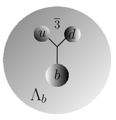
For $\Lambda_{b}$ baryon, we used Hartree-Fock method hartree1; hartree2 to solve the helium-like Hamiltonian,

where $r_{12}$ is the relative distance between two light quarks “orbiting” the heavy quark and their interaction potential is the last two terms in the equation (26) with coefficient $\alpha^{\prime}$ and $\beta^{\prime}$. For the Hartree-Fock calculation of the energy $E$, we take $\beta^{\prime}=\beta$ and $\alpha^{\prime}=0.6$ mes_q_mod.

To solve the Hamiltonian (26), we consider the trial wave function, which is space-symmetric and spin-antisymmetric, in terms of Slater determinant

where $x_{i}\equiv(\vec{r},s)$ collectively denotes the space and spin indices, $\chi_{i}(\vec{r},s)=\phi_{i\,s}(\vec{r})\,\mathcal{S}(s)$ with $\phi(\vec{r})$ being the 1S state. Therefore, the expectation value of the the Hamiltonian can be written as

where, we have used

In contrast to the helium atom, the presence of linear $r$-terms in the Hamiltonian leads to additional exchange-energy terms in the calculation. With these linear $r$-terms in, the Hartree-Fock equation becomes

We solve for $E$ in equation (29) iteratively and, eventually, the $\Lambda_{b}$ mass is calculated from

The PDG value of $\Lambda_{b}(5620)$ is obtained by setting the $m_{u/d}$ to 0.157 GeV.

In Table 3, we compare the nonperturbatively tuned $m_{u/d}$ on our lattices with those obtained by solving the equations (23) and (29). The bare lattice light quark masses cannot be directly compared to the parameter $m_{u/d}$ in these equations mainly because of the use of renormalized $b$ quark mass (in $\overline{\text{MS}}$ scheme) in the Hartree-Fock calculation. Therefore, the $m_{u/d}$’s in the above calculation return a sort of “renormalized constituent” quark mass. Nonetheless it is obvious that we need two different $m_{u/d}$ for two different systems, namely $B$ and $\Lambda_{b}$. So by comparing the two sets, we simply wish to point out that the lattice tuned $m_{u/d}$’s are in same order of magnitude as Schrödinger equation based quark model but have a difference of 10 – 15%. This helps us to understand the possible physics behind two different tunings of light quark mass in determining the masses of single bottom hadron(s) and double bottom tetraquark.

A plot of variation of $bb\bar{u}\bar{d}$ mass with various $am_{u/d}$, including the $\Lambda_{b}$ and $B$ tuned values is shown in Fig. 3. Here we make a naive comparison of our data with the earlier quark model, lattice calculations and the PDG values, and it shows an interesting trend.

Firstly, PDG $Z_{b},\,Z_{b}^{\prime}$ and the lattice states, consisting of $[bb]/[\bar{b}\bar{b}]$ heavy tetraquark systems, are clustered around two different masses. Our data at $B$-meson tuning point coincides with the PDG $Z_{b}\,(10610)$ and $Z_{b}^{\prime}$ (10650) states aligning with the idea that they decay mostly into $\bar{B}B^{*}$ and $\bar{B}^{*}B^{*}$ respectively, possibly indicating molecular nature of the state. However, our tetraquark state with $\Lambda_{b}$ tuning overlaps mostly with other lattice results indicating the possibility of capturing a bound tetraquark state $[bb][\bar{l}_{1}\bar{l}_{2}]$ much like the $b[{l}{l}]$ state of $\Lambda_{b}$. The effective masses of the states, obtained from $\mathcal{O}_{D}$ and $\mathcal{O}_{M_{1}}$, when compared with the $B-B^{*}$ threshold, we find $|D\rangle$ to exhibit a shallow bound state while $|M_{1}\rangle$ is just marginally above. The majority of the lattice results francis1; francis2; junnarkar; luka are found to be below this threshold as is obvious from the Fig. 3.

To this end, in Fig. 4 we plot the effective masses of these two states obtained at different lattice spacings. The colored bands represent fitted $am_{\mathrm{eff}}$ values. The superscripts $\Lambda_{b}$ and $B$ denote the light quark tuning. The dotted lines represent the lattice thresholds. The lattice threshold is defined as $M_{B}+M_{B^{*}}$ of the non-interacting $B-B^{*}$ system and consequently constructed entirely from $B$-meson tuned $am_{u/d}$ and $\Upsilon-\eta_{b}$ tuned $m_{b}$. We want to mention here in passing that on two occasions we used $\Lambda_{b}$ tuning for operators $\mathcal{O}_{M_{1}/M_{2}}$ – ($i$) to choose $t_{0}$ for GEVP analysis and ($ii$) to determine relative contribution to the bound tetraquark ground state.

In the Table 4, we present our results of the tetraquark states corresponding to the operators given in the expressions (14, 15, 16). We call these states $\mathcal{O}_{X}^{\dagger}|\Omega\rangle\equiv|X\rangle$ as trial states, which will later be subjected to variational analysis. The $|\Omega\rangle$ is the vacuum state. We use two-exponential uncorrelated fit to the correlation functions, the fitting range being chosen by looking at the positions of what we consider plateau in the effective mass plots. In the columns showing various lattices, we present the masses both in lattice unit $a\,E_{\textmd{latt}}$ and physical unit $M_{\textmd{latt}}$ in MeV, the notations being introduced in equation (9). The errors quoted are statistical, calculated assuming the lattice configurations of different lattice spacings are statistically uncorrelated. The second column shows the tuning used for the corresponding states. In the last column we provide the masses averaged over all the lattice ensembles.

From the Fig. 4 and Table 4 it is clear that the trial state generated by our $\mathcal{O}_{D}$ operator is below $B-B^{*}$ threshold which possibly indicates a bound state. On the other hand, the states for $\mathcal{O}_{M_{1}}$ and $\mathcal{O}_{M_{2}}$ are just above it. We tabulate the difference of the masses from their respective thresholds $\Delta M_{D/M_{1}/M_{2}}=M_{D/M_{1}/M_{2}}-M_{B}-M_{B^{*}}$ in the Table 5. In this table, we calculated the following correlator ratio to determine the mass differences which gives us an estimate of the binding energy beane,

It has been observed iritani that the expression (31) used to determine $\Delta M_{X}$ can possibly lead to false plateaus because of $B-B^{\star}$ scattering states contributing differently in $|D\rangle,\,|M_{1}\rangle,\,|M_{2}\rangle$ excited states which might persist at large $t$. In the present analysis, we have assumed these contributions are of same order of magnitude and cancel each other at moderately large $t$.

References

- (1) A.E. Bondar, A. Garmash, A.I. Milstein, R. Mizuk and M.B. Voloshin, Phys. Rev. D 84, 054010 (2011).
- (2) A. Bondar et al. (Belle Collaboration), Phys. Rev. Lett. 108, 122001 (2012).
- (3) R. Aaij et al. (LHCb Collaboration), Phys. Rev. Lett 112, 222002 (2014).
- (4) R.F. Lebed, R.E. Mitchell and E.S. Swanson, Prog. Part. Nucl. Phys. 93, 143 (2017).
- (5) A. Esposito, A. Pilloni and A.D. Polosa, Phys. Rep. 668, 1 (2017).
- (6) S.L. Olsen, T. Skwarnicki and D. Zieminska, Rev. Mod. Phys. 90, 015003 (2018).
- (7) A.V. Manohar and M.B. Wise, Nucl. Phys. B399, 17 (1993).
- (8) E.J. Eichten and C. Quigg, Phys. Rev. Lett. 119, 202002 (2017).
- (9) Y. Ikeda, B. Charron, S. Aoki, T. Doi, T. Hatsuda, T. Inoue, N. Ishii, K. Murano, H. Nemura and K. Sasaki, Phys. Lett. B729, 85 (2014).
- (10) Marc Wagner et al. 2014 J. Phys.: Conf. Ser. 503, 012031.
- (11) M. Padmanath, C.B. Lang and S. Prelovsek, Phys. Rev. D 92, 034501 (2015).
- (12) C. Alexandrou, J. Berlin, J. Finkenrath, T. Leontiou and M. Wagner, Phys. Rev. D 101, 034502 (2020).
- (13) S. Prelovsek, H. Bahtiyar and J. Petkovic, Phys. Lett. B 805 (2020) 135467.
- (14) C. Hughes, E. Eichten and C.T.H. Davies, Phys. Rev. D 97, 054505 (2018).
- (15) A. Francis, R.J. Hudspith, R. Lewis and K. Maltman, Phys. Rev. Lett. 118, 142001 (2017)
- (16) A. Francis, R.J. Hudspith, R. Lewis and K. Maltman, Phys. Rev. D 99, 054505 (2019).
- (17) P. Junnarkar, N. Mathur and M. Padmanath, Phys. Rev. D 99, 034507 (2019).
- (18) L. Leskovec, S. Meinel, M. Pflaumer and M. Wagner, Phys. Rev. D 100, 014503 (2019).
- (19) J. P. Ader, J. M. Richard, P. Taxil, Phys. Rev. D 25, 2370 (1982).
- (20) P. Bicudo, and M. Wagner, Phys. Rev. D 87, 114511 (2013).
- (21) P. Bicudo, K. Cichy, A. Peters, B. Wagenbach and M. Wagner, Phys. Rev. D 92, 014507 (2015).
- (22) P. Bicudo, J. Scheunert and M. Wagner, Phys. Rev. D 95, 034502, (2017).
- (23) P. Bicudo, M. Cardoso, A. Peters, M. Pflaumer and M. Wagner, Phys. Rev. D 96, 054510 (2017).
- (24) B.A. Thacker and G.P. Lepage, Phys. Rev. D 43, 196 (1991).
- (25) G.P. Lepage, L. Magnea, C. Nakhleh, U. Magnea and K. Hornbostel, Phys. Rev. D 46, 4052 (1992).
- (26) E. Follana, Q. Mason, C. Davies, K. Hornbostel, G.P. Lepage, J. Shigemitsu, H. Trottier and K. Wong, Phys. Rev. D 75, 054502 (2007).
- (27) A.X. El-Khadra, A.S. Kronfeld and P.B. Mackenzie, Phys. Rev. D 55, 3933 (1997).
- (28) E.B. Gregory et al. (HPQCD Collaboration), Phys. Rev. D 83, 014506 (2011).
- (29) N. Kawamoto and J. Smit, Nucl. Phys. B 192, 100 (1981).
- (30) J. Jiang, W. Chen and S. Zhu, Phys. Rev. D 96, 094022 (2017).
- (31) R.L. Jaffe, Phys. Rep. 409, 1 (2005).
- (32) P. Mohanta and S. Basak, Phys. Rev. D 101, 094503 (2020).
- (33) A. Bazavov et al., Rev. Mod. Phys. 82, 1349 (2010).
- (34) K. Orginos and D. Toussaint (MILC), Phys. Rev. D 59, 014501 (1998).
- (35) K. Orginos, D. Toussaint, and R. L. Sugar (MILC), Phys. Rev. D 60, 054503 (1999).
- (36) K. C. Bowler et al., (UKQCD Collaboration), Phys. Rev. D 54, 3619 (1996).
- (37) B.C. Tiburzi, Phys. Rev. D 71, 034501 (2005).
- (38) Z.S. Brown, W. Detmold, S. Meinel, and K. Orginos, Phys. Rev. D90, 094507 (2014).
- (39) S. Godfrey and N. Isgur, Phys. Rev. D 32, 189 (1985).
- (40) S. Capstick and N. Isgur, Phys. Rev. D 34, 2809 (1986).
- (41) folk.uib.no/nfylk/Hartree/lindex.html
- (42) D. R. Hartree and W. Hartree, Proc. R. Soc. Lond. A150: 9–33, (1935).
- (43) V. Fock, Z. Physik 61, 126–148 (1930).
- (44) Marek Karliner and Jonathan L. Rosner, Phys. Rev. Lett. 119, 202001 (2017)
- (45) M. Tanabashi et al. (Particle Data Group), Phys. Rev. D98, 030001 (2018) and 2019 update.
- (46) S.R. Beane, K. Orginos, and M.J. Savage, Phys. Lett. B 654, 20 (2007).
- (47) T. Iritani et al. (HAL QCD Collaboration), JHEP 1610 (2016) 101.
- (48) G. Yang, J. Ping, and J. Segovia, Phys. Rev. D 101, 014001 (2020)