August 11, 2026
Global Stability and Periodicity in a Glucose-Insulin Regulation Model with a Single Delay
M. Angelova1, G. Beliakov1, A. Ivanov2, and S. Shelyag1
1 School of Information Technology, Deakin University Geelong, Australia
2 Department of Mathematics, Pennsylvania State University, USA
Keywords: delay differential equations,
linearization,
stability analysis,
limiting interval maps,
global asymptotic stability,
existence of periodic solutions,
diabetes.
Abstract
A two-dimensional system of differential equations with delay modelling the glucose-insulin interaction processes in the human body is considered. Sufficient conditions are derived for the unique positive equilibrium in the system to be globally asymptotically stable. They are given in terms of the global attractivity of the fixed point in a limiting interval map. The existence of slowly oscillating periodic solutions is shown in the case when the equilibrium is unstable. The mathematical results are supported by extensive numerical simulations. It is deduced that typical behaviour in the system is the convergence to either a stable periodic solution or to the unique stable equilibrium. The coexistence of several periodic solutions together with the stable equilibrium is demonstrated as a possibility.
1 Introduction
This paper deals with further qualitative and numerical analyses of the Sturis-Bennett-Gourley model of the glucose-insulin interaction in the human body. The model was proposed in [4] as a simple two-dimensional system of nonlinear differential equations with one delay. It can also be viewed as an abbreviated simplified version of a more complex differential model with two delays [28, 29].
Only a limited number of parameters of the physiologically closed glucose-insulin interaction system are accessible for direct measurements. Therefore, mathematical modelling is required to facilitate the estimation of the narrow physiological range of the glucose-insulin system components [35]. The physiological time delay plays an important part in the regulation and the feedback of the system and determines the important properties of the mathematical description of the model.
The glucose-insulin regulatory system is a key component in the metabolism of the human body. The pancreas and the liver regulate the production of insulin and glucose respectively in order to maintain normal level of the blood glucose. Failure to do this can result in high blood sugar and diabetes which is related to many other long term health problems. Within this regulation, both rapid (period mins) and ultradian (period mins) oscillations of insulin have been observed [38], along with glucose oscillations (period mins) [39]. The ultradian oscillations were first discovered by Hansen [16] and observed during fasting, meal ingestion, continuous enteral nutrition and constant glucose infusion.
Due to the monotone nature of the nonlinearities involved in the two-dimensional system it is a natural conjecture that some degree of the simplicity in the dynamical behaviour of the solutions should be observed in the model. Such simpler dynamics would be consistent with known behaviours in scalar differential delay equations with monotone nonlinear feedback [33, 34, 42]. In fact, some of the known theoretical results can be extended to the Sturis-Bennett-Gourley model (see further details in the next section Preliminaries).
The primary objective of this paper is to derive conditions for the global asymptotic stability in the model as well as conditions for the existence of nontrivial periodic solutions. We apply and further develop some of our earlier approaches and results to study differential delay equations and systems via underlying finite-dimensional discrete maps [8, 14, 22, 23]. In our analyses in this paper we also use prior related results, in particular those obtained in [4, 5, 6, 32, 33, 34]. The differential delay model we consider was introduced and studied in paper [4]. We further investigate its properties and interpret some of them from an alternative prospective via a limiting interval map. The principal result of paper [33], an extension of the Poincaré-Bendixson Theorem [37, 3, 9] to delay differential equations, can be applied to the Sturis-Bennett-Gourley system as well. As a result one can conclude that its every solution converges to either the unique equilibrium or to a periodic solution. In this paper, we demonstrate various possibilities of such eventual dynamics through several numerical examples.
The approach we propose to analyse the system is through a limiting one-dimensional map, which is formally obtained from the original differential delay system when the delay goes to infinity. The resulting interval map is relatively simple: it is given by a monotone decreasing function and can only have a unique fixed point and cycles of period two (which can be either attracting, or repelling, or a combination of the two possibilities).
The dynamics of the limiting interval map largely determine the dynamics of our two-dimensional differential delay system. When the only fixed point of the interval map is globally attracting then the corresponding unique steady state of the delay system is also globally asymptotically stable (for arbitrary delay ). However, when the only fixed point of the interval map is repelling the dynamics in the differential delay system are varied and dependent on the size of delay . When the delay is small enough, for some , the unique equilibrium of the differential delay system is locally asymptotically stable. Note that only the local stability of the equilibrium can be claimed, as examples are possible that the delay system has stable periodic solutions away from the stable constant equilibrium (see an example in Section 4). When the delay becomes large enough, for some , then the differential delay system has a slowly oscillating periodic solution. In this case the corresponding characteristic equation of the linearised system about the steady state has a leading pair of complex conjugate solutions with the positive real part and the imaginary part within the interval . This leading eigenvalue makes the slow oscillation in the system typical, in agreement with known results for the case of similar scalar differential delay equations [34, 42].
It is important to note that from the mathematical point of view there is no uniqueness in the model for stable periodic solutions or for the stable equilibrium. We construct explicit examples of our two-dimensional differential delay system when the coexistence of two stable periodic solutions is observed (Section 4). We also demonstrate the possibility when a stable periodic solution coexists together with the locally stable equilibrium (Section 4). The examples are easily generalised to the case when any finite number of stable periodic solutions can coexist with or without the locally attracting equilibrium. This multi-stability phenomenon implies the utmost importance of the proper choices of the nonlinearities when the differential delay system is suggested as an actual model of a particular applied problem. For some of such known and available in the literature models we numerically observe the uniqueness of the stable periodic solution and its global attractivity within the admissible set of initial conditions.
The novelty of our approach is that we derive a simple one-dimensional dynamical system (interval map) and use it to determine the global dynamical properties of our infinite-dimensional dynamical system with delay. The typical dynamical behaviours in our model are also simple - it is the convergence to either a stable periodic solution or to the unique stable equilibrium, or a combination of such behaviours.
The paper is organised as follows. Section 2 describes the foundations of the mathematical problem. It includes references to and a brief review of existing closely related results obtained by others. In Section 3, we derive the main analytical results, which are then numerically confirmed in Section 4. A concluding summary and a brief discussion are given in Section 5.
2 Preliminaries
2.1 Differential Delay Model and Assumptions
Consider the system of differential equations with delay [4],
| (1) | |||||
where and represent the relative concentrations of insulin and glucose, respectively, is the insulin degradation rate, is the external glucose input. The function corresponds to pancreatic insulin production, dependent on glucose concentration, and is the glucose consumption by the brain. The third term in the second equation represents the insulin-dependent glucose utilisation in the muscles, while the last term, , represents the hepatic glucose production. is the time delay between plasma insulin production and its effect on hepatic glucose production.
The system is considered under the following assumptions:
- (H1)
Functions are non-negative and continuously differentiable for , with defined as for convenience. Real parameters are all positive;
- (H2)
and ;
- (H3)
and ;
- (H4)
and ;
- (H5)
and .
The assumptions (H1)-(H5) are derived from and justified by the physiological mechanisms of the glucose-insulin interaction in the human body, see e.g. papers [4, 5, 28, 29] for additional details.
The phase space of system (1) is defined as where . For arbitrary initial function the corresponding solution to system (1) can be constructed by the standard step methods [2, 11, 15]. We assume that such solutions exist for an arbitrary initial function and all (which is the case under the assumptions that nonlinearities are continuously differentiable).
It is an easy observation that positive initial data for system (1) result in solutions that are positive for all . More precisely, if the initial function is such that and then and holds for all (see further details and proof in [4]). It can also be shown that both components and of all solutions to system (1) are bounded from above and bounded away from zero. Moreover, a stronger property called the persistence can be established here. It says that positive constants and can be identified, independent of particular initial data, such that for an arbitrary initial function and the corresponding solution to system (1) there exists a time moment such that the following holds
| (2) |
These and other basic properties of the solutions are proved in [4] as Propositions 2.1, 2.2, and 2.4. We will revisit them later in the paper from a different point of view.
2.2 Linearization and Characteristic Equation
In this subsection we present well-known facts about the unique positive equilibrium of system (1), the linearized system about the equilibrium, and the characteristic equation of the linear system. More related details can be found in papers [4, 5] and [28].
Equilibria of differential delay system (1) are found by solving the nonlinear system
| (3) |
which reduces to a single scalar equation for : . It is straightforward to see that the latter has a unique positive solution , implying that the original system (1) has a unique equilibrium where .
The linearized system about the positive equilibrium has the form
| (4) | |||||
Note that system (4) is also the linearization of the translated system (7) (derived in subsection 2.4). The characteristic equation of the linear system (4) has the form
| (5) |
where Since and then
The form (5) of the characteristic equation allows us to use known facts about its properties derived elsewhere, see e.g. [1, 8, 28]. The stability/instability of the zero solution of system (4) is determined by the location of the solutions of the characteristic equation (5) in the complex plane. If all solutions of the characteristic equation have negative real parts (or are negative themselves) then the zero solution of (4) is asymptotically stable. If the characteristic equation (5) has a complex conjugate solution with the positive real part then the zero solution of (4) is unstable. In the latter case there exists the so-called leading pair of complex conjugate solutions of the characteristic equation (5), where and . The leading means that is the largest real part among all solutions of (5). All other complex conjugate solutions of (5) satisfy and . See Lemma 1 of [1] and Lemma 3 of [8] for more details and proofs.
The described above stability or instability of the zero solution of the linear system (4) in terms of the eigenvalues of the characteristic equation (5) carry over to the nonlinear system (1). The constant solution of the latter has the same type of stability as of the linear system provided all the nonlinearities are -smooth in a neighborhood of (see [17], Chapter 9, for further details and proof).
One of the main questions of interest in this paper is about the typical behaviour of solutions in system (1). In view of the strong monotonicity properties of the nonlinearities and some of the previously obtained results are applicable and can be used in our analysis. The main result of paper [33], Theorem 2.1, implies that for every initial function the corresponding solution converges as either to a periodic solution or to the unique equilibrium of system (1). The follow-up question is which of these possible behaviours are typical, and which ones can be observed in numerical simulations. It turns out that both stable periodic solutions or a stable equilibrium or a simultaneous coexistence of both are typical (as shown numerically in section 4). It is also evident that there exist unstable periodic solutions (e.g. those separating neighboring stable periodic solutions; they usually cannot be observed numerically).
Oscillatory solutions in differential delay systems are typical in general. It is a known fact that all solutions to system (7) oscillate when the characteristic equation (5) has no real eigenvalues [8] (also see Proposition 3.10 of subsection 3.4). Due to the overall negative feedback the slow oscillation can be typical in system (1) (see the related definition 3.9 in subsection 3.10). In particular, initial functions with give rise to slowly oscillating solutions. This oscillation is typical as small perturbations of such initial functions leave them within the same initial set.
Another possibility for a typical behaviour is that solutions converge monotonically to the equilibrium as . This is the case when the characteristic equation (5) has real eigenvalues (which are then necessarily negative). Such a case implies the existence of the exponential decaying solutions to the linear equation (4), and also the existence of solutions close to the exponential ones for the nonlinear system (1).
The results of papers [31, 34, 42] for scalar equations suggest that typical behaviour of the oscillating solutions in system (1) is the eventual slow oscillation. That is, for almost all initial functions the corresponding solution is slowly oscillating for for some This means that if an initial function is such that the solution is not slowly oscillating for then its every neighborhood contains an initial function such that the corresponding solution is eventually slowly oscillating.
Note that the problem of typical behaviour in a differential delay system is a very challenging one in general (many aspects of this problem remain unsolved even for the scalar case of a simple single equation; the basic paper [34] on the issue exists in a preprint form only). Therefore, we are in a position in this paper to only numerically verify the assumed theoretical results about the typical behaviours. The rigorous mathematical proofs will hopefully be accomplished at a later time.
2.3 Related Interval Maps
In this subsection we recall some basic notions and definitions on interval maps related to the needs of this paper. Comprehensive expositions on the theory of one-dimensional maps can be found e.g. in monographs [10, 40].
Given a continuous map of a closed interval into itself a forward trajectory through an initial point is defined as the set where is the iteration of (). A set will be called invariant under if . Note that a proper inclusion is allowed under this definition.
Definition 2.1.
(i) A fixed point of a continuous map of an interval into itself is called if there exists an open interval such that , , and for every point one has that holds.
(ii) The largest connected interval with this property is called the domain of immediate attraction of the fixed point .
(iii) A point is called periodic with period if and for every .
The corresponding set is called a cycle of period .
Clearly that every point of the cycle is periodic of period for the map ; it is also a fixed point for the map .
The following statement is a well-known simple fact in the theory of interval maps. Its proof easily follows from related facts of Section 2.4 in [40].
Proposition 2.2.
For an arbitrary point in the domain of immediate attraction of the fixed point there always exists a closed finite interval such that , and
Definition 2.3.
Let be an attracting fixed point of a continuous map . An infinite set of intervals will be called a squeezing sequence of imbedded intervals if the following holds:
It is evident that the sequence of intervals in Proposition 2.2 is a squeezing imbedded sequence. Given an initial point in the domain of immediate attracting it is also clear that a squeezing imbedded sequence of intervals containing its iterations always exists but is not uniquely defined in general.
2.4 Translation to Zero Equilibrium
It was demonstrated in [4, 5] that under the assumptions (H1)-(H5) the system (1) has unique equilibrium where and is a unique positive solution of the nonlinear equation . As a matter of convenience, for various theoretical considerations and computational tasks of this paper it is advantageous to have this equilibrium shifted to the zero equilibrium state . One of the reasons for this need is that the equilibrium depends on all the parameters and functions involved in system (1). Such shift is achieved by the change of the dependent variables by
| (6) |
System (1) is then transformed into the following one:
| (7) | |||||
where Functions are strictly monotone increasing and satisfying the positive feedback condition for . Function is strictly decreasing and satisfying the negative feedback assumption for . System (7) has the unique zero equilibrium .
3 Main Results
3.1 Limiting Interval Map
In this sub-section we derive a limiting interval map for the differential delay system (1) as . First we transform system (1) to one with the normalised delay by rescaling the independent variable by . It is a straightforward calculation then that reduces system (1) to the following form
| (8) | |||||
By taking the limit as the latter becomes a system of functional difference equations:
| (9) |
which in turn is further reduced to a single scalar difference equation for the variable :
| (10) |
It is easy to see, based on the assumptions (H1)-(H5), that the function in the left hand side of equation (10), , satisfies:
| (11) |
Likewise, the function in the right hand side of equation (10), , satisfies:
| (12) |
Therefore, the inverse function exists, and equation (10) can be explicitly solved for as follows:
| (13) |
where the composite function is defined and continuous on . Besides, due to assumptions , function is continuously differentiable on with
| (14) |
The values are easily calculated as:
| (15) |
The asymptotic properties of solutions of equation (13) are completely determined by the dynamical properties of the iterations of the interval map . A comprehensive theory of such equations is given in the monograph [41]. All relevant properties on interval maps can be found in monographs [10, 40].
3.2 Principal Results
Based on property (14) we can build a sequence of imbedded intervals for map as follows. Set and Proceed then recursively as Define the limiting set by .
The set is either a single point or a closed interval with a non-empty interior. In the first case one has that . In the second case the endpoints form a cycle of period two: .
The sequence of imbedded interval for the component generates the sequence of imbedded intervals for the component through the first difference equation of system (9) by .
We shall formally distinguish the following subcases for the set and its structure:
-
The set is a single point . It is the only fixed point of the interval map which is then globally attracting on : for every initial point one has ;
-
The set is a closed non-empty interval . Then and is a cycle of period two, with . Assume also that the two-cycle is globally attracting: for every initial point its forward iterations converge to the cycle: as . In addition, it is assumed that the generic condition holds;
-
The set is an interval formed by a cycle of period two which is locally attracting only. In addition, it is assumed that the condition holds;
-
The set is an interval formed by a cycle of period two. In addition, the fixed point is locally attracting: there exists an interval such that for every initial point one has ;
Below we state the principal results of this paper which are essentially dependent and built based on the structure of the limiting sets of the map as described above by properties .
Theorem 3.1.
Suppose that in addition to assumption holds. Then for every delay the unique equilibrium of system (1) is globally asymptotically stable: for an arbitrary initial data the corresponding solution satisfies: .
Theorem 3.1 is a strong delay independent result about the global asymptotic stability of the unique equilibrium of system (1) with infinite-dimensional phase space based on the global attractivity of the corresponding fixed point in a simple limiting interval map defined by the real-valued function . Theorem 3.1 is proved in subsection 3.3 (as Theorem 3.8).
Note that a closely related result to Theorem 3.1 is proved in paper [4] as Theorem 3.2. However, their approach and method of proof are different from what we use in present paper. We reflect more on paper [4] in the Conclusion section.
Theorem 3.2.
Suppose that in addition to assumption holds. Then there exists such that for every delay system (1) has a slowly oscillating periodic solution.
The slow oscillation of solutions here means that both components and are slowly oscillating functions about their respective equilibrium values and . Therefore, and are slowly oscillating functions with their successive zeros separated by a time span larger than the delay . For more complete definitions and statements see details in Subsection 3.4.
Under assumption the cycle is globally attracting on : for every initial value the sequence of its iterations is attracted by the cycle as . This means that both sequences and are monotone and converge to either or (depending on the location of in relation to the fixed point ). To show the existence of a slowly oscillating periodic solution to system (1) we use the standard and well developed techniques of the ejective fixed point theory [11, 15]. To that end the main points we have to show holding true for system (1) are:
- (i)
Construction of a cone of initial data for system (1) and a non-linear map which maps the cone into itself. The map usually is an appropriately defined shift operator along the solutions;
- (ii)
Existence of a leading eigenvalue to the characteristic equation (5) with the largest positive real part and the imaginary part within the range ;
- (iii)
The compactness of the shift operator along solutions of the system starting on the cone.
The outline of the proof of the existence of periodic solutions is given in Subsection 3.4.
Note that in general the ejective fixed point techniques do not address the issue of the uniqueness of the slowly oscillating periodic solution. The existence of periodic solutions can only be proved; the periodic solutions can be non-unique in many cases. This is true for all the classes of delay equations and systems to which they were applied, including our system (1). However, the uniqueness of the globally attracting cycle of period two for the one dimensional map seems to yield the uniqueness of a stable slowly oscillating periodic solution to system (1). This fact can be verified numerically. We have done it for two classes of the nonlinearities used in applications: Hill type functions [19] and exponential functions [29].
Theorem 3.3.
Suppose that in addition to assumption holds. Then there exist multiple choices of the nonlinearities and of the parameter values such that system (1) possesses at least two slowly oscillating periodic solutions.
The key assumption in is that the two-cycle is locally attracting only; therefore, there exists another cycle of period two. Since the fixed point is repelling. Hence, there exists the minimal cycle of period two, , such that the open interval is attracted to it. In addition, the inequalities hold. Both cycles and are at least one-sided attracting. The structure of the map on the set can be arbitrary; however, since is monotone decreasing, it can only contains additional cycles of period two.
The non-uniqueness of the two-cycle , and the existence of the second two-cycle , seem to be an important factor for the existence of multiple periodic solutions to system (1). We construct an example of system (1) when it has one slowly oscillating periodic solution related to the smallest two-cycle and the second slowly oscillating periodic solution related to the largest two-cycle (see an example in subsection 3.5). Such example can be easily generalized to produce any finite number of slowly oscillating periodic solutions to system (1).
Theorem 3.4.
Suppose that in addition to assumption holds. Then there exist multiple choices of the nonlinearities and of the parameter values such that system (1) possesses both a slowly oscillating periodic solution and the locally attracting equilibrium .
The principal difference between Theorem 3.4 and Theorem 3.3 is that the fixed point is attracting for the map in the latter (while it was repelling for the former). Therefore, its minimal two-cycle is one-sided repelling with the interval being the domain of immediate attraction of the fixed point . This fact makes the equilibrium locally attracting for the system (1). Outside the interval the structure of the map can largely be preserved to be the same as in Theorem 3.3. This would guarantee the existence of a slowly oscillating periodic solution associated with the two-cycle . As in the case of Theorem 3.3 the example can be easily generalized to produce any finite number of periodic solutions, while remains a locally attracting equilibrium. The phenomenon described by Theorem 3.4 is demonstrated by an example of numerical solution of the system (7) in Subsection 3.5.
3.3 Invariance, Persistence, and Global Asymptotic Stability
Suppose that map has a closed finite interval invariant in the general sense , and let interval be defined by . Consider the following subset of the phase space :
It is easily seen, based of the properties of functions and , that the map has an invariant interval such that for an arbitrary initial value its first iteration under , satisfies . Indeed, the interval can be defined as , where the finite interval is the image of the positive semi-axis under the map . The values of and are given as . The corresponding interval is then defined as .
The following statement describes the fact that the solutions of system (1) with initial functions in the set remain within this set for all forward times .
Lemma 3.5.
(Invariance) Suppose that an initial function is such that , where is a closed interval invariant under map . Then the corresponding solution of system (1) satisfies for all .
Lemma 3.5 shows that when the initial data for system (1) is such that and then the components and of the corresponding solution to system (1) satisfy the inclusions:
Proof.
The proof of Lemma 3.5 can be done by induction in time by using the cyclic structure of system (1). We provide its outline below.
Suppose that the initial function for system (1) is given such that and . Assume first that for some . Then also is satisfied. Indeed, suppose is the first time moment of exit of the component from the interval . To be definite assume first that and and for some . Then since Therefore, , a contradiction with .
In the case when and there exists a sequence of -values such that and . This would imply that the derivative is positive in a small right neighborhood of , a contradiction with being the first point of exit from interval .
Given and we shall show next that . This is done in a way similar to the reasoning for the component above. Assume is the first point of exit of the component from the interval . To be specific let and holds. Using the monotone nature of functions and one sees that . Therefore, a contradiction with . The case when holds at the first point of exit from interval is treated similarly to the analogous case for by selecting a sequence with and .
The proof can now be completed by induction in with a step . Since then also These values of and are considered next as new initial data for the same solution to derive the inclusions , and so on. ∎
From the proof of Lemma 3.5 it is seen that for every initial data there exists a time moment such that the corresponding solution satisfies
| (16) |
Indeed, if at some then due to reasons in the first part of the proof of Lemma 3.5. Likewise, if for some . Therefore, one has to consider the possibility that and . To be specific assume that and for all (other options are treated along the same line). Then the respective equations of system (1) imply that and for all Therefore, the finite limits exist. By applying the limit to both equations of (1) along these components of the solution one sees that satisfies the equilibrium equations:
Therefore, is the only equilibrium of system (1), so that and . This is a contradiction with the inequalities and , since and belong to the interior of the intervals and , respectively.
The reasoning above leads to the following
Proposition 3.6.
(Uniform Persistence I) There are positive constants and such that for every initial data there is a time moment such that the corresponding solution of system (1) satisfies
Indeed, as it is seen from the above reasoning the values of the constants can be chosen as
We can now apply an inductive argument to the chain of reasoning preceding Proposition 3.6. Since and then and This is shown exactly the same way as the inclusions (16). By the induction reasoning, there exists a sequence of -values, such that
| (17) |
The crucial role for the asymptotic behaviour of solutions is now played by the structure of the set . Note that the imbedded sequence of intervals , and the limiting set were constructed in Subsection 3.2. The following two possibilities can only happen.
(I) The set is a closed interval with non-empty interior. Then points form a cycle of period two under the map . It is the maximal cycle of period two for the map in the sense that any other cycle of period two belongs to the open interval Also, the cycle is at least one-sided attracting (from above). The latter means that for every initial value one has that is an increasing sequence with . Likewise, for every initial value the sequence is decreasing with . Therefore, in this case, the persistence property of Proposition 3.6 can be essentially improved. Denote the interval . The following property holds:
Proposition 3.7.
(Uniform Persistence II) For arbitrary initial data the following holds for the corresponding solution
The proof immediately follows from the property (17). In fact, more precise inequalities also hold under the assumptions of Proposition 3.7:
A proof of the latter requires certain preliminaries and details which cannot be included in the paper due to their length.
(II) The set is a single point. This implies that and that the fixed point is globally attracting on for the map . In this case one has that the following global asymptotic stability property holds for system (1).
Theorem 3.8.
(Global Asymptotic Stability, also Theorem 3.1) Suppose that the unique fixed point of the interval map is globally attracting: for every . Then the unique constant solution of system (1) is globally asymptotically stable: for arbitrary initial function and every delay the following holds for the corresponding solution
Again, the proof immediately follows from inclusions (17).
Remark. Note that a uniform persistence property of all solutions of system (1) is also proved in [4], see Proposition 2.4 there. However, our uniform persistence results, given by Propositions 3.6 and 3.7, provide explicit lower and upper bounds for the components and in terms of one-dimensional map (therefore, in terms of functions and parameters ). In fact, the bounds given by Proposition 3.7 are best possible in certain circumstances, e.g. when . They are given in terms of the maximal cycle of period two for the map .
Paper [4] also contains a condition for the global convergence to the equilibrium value of the component of system (1). It is given by Theorem 3.2 there, which requires that the following system for and
| (18) |
has no solutions . This is related to our more general and transparent condition of Theorem 3.8, about the global asymptotic stability in (7), which simply requires that the fixed point of the map is globally attracting. If the later is satisfied then system (18) has no solutions , since the existence of such a solution would mean that the pair forms a cycle of period two for the map , contradicting the global attractivity of its fixed point . In fact, it can be showed, with some additional effort, that under the assumptions imposed on system (1) the only fixed point of map is globally attracting if and only if system (18) has no positive solutions.
3.4 Periodic Solutions
In this subsection we outline the algorithm how the existence of periodic solutions for system (1) can be derived. It follows the well established techniques of the ejective fixed point theory, see [11] and [15] for general theoretical basics; we also use some related specific details from papers [1, 8, 20, 21, 22] to show the periodicity.
The basic components for the existence of periodic solutions are:
- (1)
Construction of a cone of initial functions, and a translation operator along solutions on it (Poincaré map), such that its fixed points give us slowly oscillating periodic solution. Some of these will have to be verified numerically;
- (2)
The instability of the zero solution of the corresponding linearized system. This can be derived from the characteristic equation in terms of the existence of a pair of complex conjugate solutions with positive real part. Known results can be used here with proper harvesting and compilation, e.g. those in [1, 8, 20];
- (3)
The compactness of the nonlinear map constructed in step (1) above. This is rather straightforward derivation based of the boundedness and smoothness properties of the nonlinear functions given in assumptions ;
- (4)
Application of known results for the existence of periodic solutions for systems similar to (1). In particular, application of the well established ejective fixed point theory to our case;
The proof of existence of periodic solutions to system (1) (or equivalent system (7)) uses well established theory of the ejective fixed point techniques applied to specially constructed maps on subsets of initial functions of the phase space. The subsets are usually cones of the initial functions generating the so-called slowly oscillating solutions. The related maps are appropriately constructed shifts along corresponding solutions. The general theory of such approach is described in e.g. [11, 15]. In addition we shall use specific cases and results obtained in papers [1, 8, 20, 21, 22].
Definition 3.9.
(i) Given delay a continuous function is called slowly oscillating (with respect to zero) if the distance between any two of its zeros is greater than ;
(ii) A solution of system (1) is called slowly oscillating for if each of the functions and is slowly oscillating (with respect to zero in the sense of part (i)).
In case when (ii) holds each of the components and is viewed as slowly oscillating function with respect to its constant component of the unique equilibrium of system (1).
We need a sufficient condition which guarantees the oscillatory nature of all solutions to system (1). We can use the corresponding result of paper [8], see Theorem 1 there.
Proposition 3.10.
For the remainder of this subsection we shall assume that the conditions of Proposition 3.10 are satisfied.
Cone. Consider the following set of initial functions :
is a cone on .
Proposition 3.11.
Suppose that the characteristic equation (5) has no real solutions and the initial function is such that . Then the corresponding solution of system (1) is slowly oscillating in the sense that each component and is slowly oscillating. Moreover,
- (i)
The component has a sequence of zeros such that and for all . In addition, for and for ;
- (ii)
The component has a sequence of zeros such that and for all . In addition, for and for ;
- (iii)
The two sequences of zeros for and satisfy the following relationship:
with for all
Main claims of Proposition 3.11 are proved along the lines of similar propositions for other classes of equations; see e.g. [13] for scalar equations, and [20, 21, 22] for systems. We are still missing several details of a rigorous mathematical proof of this proposition; however, we have extensively verified it numerically for various choices of nonlinear functions .
Mapping on Cone. Proposition 3.11 allows one to define a nonlinear map on the cone in the following way. Given initial function consider the corresponding solution to system (1). Given its second zero consider the first component at time as an element of the Banach space , i.e . Then and , due to Proposition 3.11. Therefore, the mapping
| (19) |
maps cone into itself. The mapping is well defined for any , different from the identical zero. For the trivial initial function one defines , by the continuity of the map .
It is an easy observation that a nontrivial fixed point of the map , , gives rise to a slowly periodic solution of system (1). However, the map always has the zero as the trivial fixed point (which results in the identical zero solution to system (7) for ). Therefore, one is interested in finding fixed points of map which are different from the trivial zero one. This is done by application of the well developed theory of the ejective fixed point theory, which has been applied to various classes of functional differential equations elswhere.
Compactness and Boundedness. An important property required of map in the ejective fixed point theory is its compactness and boundedness. It is a well known basic fact that that a shift operator along solutions of retarded differential delay equations is compact [11, 15]. The boundedness of easily follows from the invariance property, Lemma 3.5. One sees that for arbitrary its first image under satisfies and (where the intervals are defined earlier). Thus the set is uniformly bounded from above and below. Alternatively, one can also start with a bounded convex part of cone , requiring that elements satisfy and .
Ejectivity. The jectivity of map can be determined in terms of a linear operator calculated on specific eigenvalues of the linearized system (4) [11, 15]. It has a closed form in a general case [22]. In lower dimensions of scalar equations or delay systems of two equations the property of ejectivity is eventually reduced to the existence of solutions of the characteristic equation (5) with positive real part and the imaginary part within the range [1, 13, 20, 21].
We shall show next that for all sufficiently large delays the characteristic equation (5) has a pair of complex conjugate solutions with the positive real part and the imaginary part satisfying . This would imply the ejectivity of the above map .
It is more convenient to rewrite the characteristic equation (5) in an alternative form by rescaling the time to get the normalized delay (see subsection 3.1, system (7)). One derives the following
| (20) |
where is a small parameter when is large enough. By setting one gets the equation , which has a pair of complex conjugate solutions , where . Consider now the characteristic equation (20) for small . By Rouché’s Theorem it has a pair of complex conjugate solutions such that is close to and is close to . We shall show that for all sufficiently small . One rewrites the characteristic equation (20) for the solution in the form
and considers its imaginary part:
By differentiating the last equation with respect to and setting one finds
which proves that for all sufficiently small , since .
3.5 Multiple Periodic Solutions
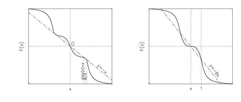
We will demonstrate numerically the existence of multiple periodic solutions using system (7). We start with linear functions , , and , which contain a constant function . The only non-linear function is then , which is monotonically decreasing (see system (21) below). The two-dimensional system of this type is simply looking and close in a sense to a single scalar differential delay equation where the non-uniqueness of slowly periodic solutions is known by several publications [23, 36]. Having derived multiple periodic solutions for system (21) we will perturb it by the inverse tangent function to produce a system of type (25) which will have the same two periodic solutions, however, they are slightly perturbed compared with those in system (21).
With the first step, system (7) becomes
| (21) | |||||
where for . Here, we will consider two appropriate choices of the monotonically decreasing designed as follows:
| (22) |
where, and are positive arbitrary constants. For this definition, is the solution of the equation . Therefore, the function is continuous (but not ) and odd by construction.
Another choice of function is as follows:
| (23) |
The function plots are shown in Fig. 1. These choices allow us to demonstrate the presence of multiple periodic solutions of different types. The first choice (Equation (22)) leads to two different periodic solutions, while the second choice (Equation (23)) to an attracting equilibrium and oscillating periodic solutions of system (7), as demonstrated by numerical solutions in Section 4.
We verify Theorem 3.1 numerically in Section 4. We make a small modification to system (21) so that it can be viewed as the original system of the form (7).
We change function from a constant to a monotonically increasing function with . For such one can choose:
| (24) |
where , and are constants, and .
We consider an intermediate system (between (7) and (21)), as follows:
| (25) | |||||
where is a constant comparable to and is chosen as from equations (22) and (23).
By replacing the constants and in equation (25) with non-linear piecewise continuous functions, linearly proportional to the argument in its range within the span of the periodic solutions and equal to constants outside this range, and by replacing outside the range of by a symmetric smooth nonlinearity with a finite limit for an appropriate , the system (25) is converted back to the original form (7).
Remark. The existence of any number of stable slowly oscillating periodic solutions can be achieved in two different ways.
(i) An analogous construction to that of function given by (22) can be continued on the interval beyond the amplitude of the second large periodic solution. Indeed, given and such that the second periodic solution exists, one finds the unique value such that it solves the equation . Then one defines function such that for and for , and for . Exactly as with given by (22) it can be showed for the modified that there exists large enough such that system (25) has three slowly oscillating periodic solutions, with the amplitude of the largest one greater than . This procedure of additional modification of in (22) can be continued step-by-step further so that one can obtain any finite number of stable slowly oscillating periodic solutions. If the procedure is applied to function given by (23) then one derives any number of stable periodic solutions together with the locally stable equilibrium.
(ii) It is known that the existence of stable (hyperbolic in general) slowly oscillating periodic solutions persists under small continuous perturbations of the non-linear right hand side (functions and constants for systems (21) and (25)) [26, 27]. Therefore, if the nonlinearity in (22) is replaced, in a sufficiently small neighborhood of , by an arbitrary and small function , and remains the same outside the small vicinity, for , then the two stable slowly oscillating periodic solutions will persist, having changed only a little. The replacement of for can be done in such a way that the resulting function is monotone decreasing there (therefore, it is monotone decreasing for all ). We now consider function by (22) on the interval where is defined above in part (i). Rescale it next to the interval by . We now use the above to replace the original in the delta neighborhood of . The resulting nonlinearity is now such that the corresponding system (25) has four stable slowly oscillating periodic solutions: two are the perturbed original periodic solutions, and the other two are small scaled original periodic solutions placed in the -neighborhood of . This procedure can be repeated any finite number of times.
4 Numerical Analysis
Analytical investigation of systems of delay-differential equations and, in particular, system (1), with biologically-inspired functions and experimentally measured parameters, is usually very difficult or impossible. Therefore numerical methods have to be employed to study the details of behaviours of the glucose-insulin regulation models [12]. Li, Kuang and Mason [29] performed numerical analysis of a two-delay glucose-insulin regulation system to analyse the dependence of bifurcations in the system on delays. This model utilised functions in their exponential forms with experimentally determined constants. In papers [19, 18] numerical analyses are performed on a similar system with more complex Hill functions, allowing for more realistic modelling of the physiological mechanisms of glucose-insulin regulation. They also studied the sensitivity of the solutions to the values of Hill parameters used and performed simulations, which represented glucose-insulin regulation disorders, namely both Type 1 and Type 2 diabetes. Here we also use numerical analysis to further clarify some of the analytical results, obtained in the previous sections.
There are two main points we aim at to demonstrate numerically. First, we demonstrate usability of equation (10) in diagnostics of the solution behaviour of system (1). Then we revisit the statement on relative insignificance of the actual forms of functions [24] in comparison to their shapes.
4.1 Numerical Methods
To confirm the results obtained in the previous sections, we produce numerical solutions for systems (1), (7), (25) and equation (10). Furthermore, some of the theoretical concepts and results obtained in Section 3 cannot be proven analytically, therefore we use numerical methods to verify their validity.
The initial value problem to system (1) is solved by using a 4-th order Runge-Kutta-Fehlberg method with an adaptive time step. The solution examples and their corresponding phase portraits are shown in Figures 3 and 4, which represent a periodic and an asymptotically stable solutions, respectively.
The delay term in the system is interpolated using Lagrange polynomials in their barycentric form [7]. This method demonstrates 4-th order self-convergence for sufficiently small time steps for both periodic and asymptotically stable solutions and a wide range of delays (see Figure 5).
To demonstrate applicability of the limiting interval map analysis, described in Subsection 3.1, we numerically solve Equation (10). The solution of the (implicit with respect to ) difference equation (10) is preferential for numerical treatment as it does not require numerically inverting a function on an arbitrary range of its argument, despite equation (13) being mathematically simpler and providing an explicit solution for .
Since the functions - are monotone, numerical solution of the difference equation (10) for does not represent difficulties, and a simplest bisection method has been implemented. To distinguish numerically the solution types is also straightforward, as the period of the solution (if such period exists) is always 2 by construction. A solution is considered periodic for a large integer if and , where is a constant, which determines the precision.
The solution of equation (10) either exhibits an asymptotic stability, which corresponds to the asymptotically stable regime for any delay in system (1), or an oscillatory function with a period 2. The latter case corresponds to the periodic solution of system (1), which exists for the delay greater than some critical value , determined numerically from the full solution of system (1) given a set of its parameters. If , the system shows a stable equilibrium solution. Examples of solutions to equation (10) are shown in Fig. 2.

Other advantages of using equation (10) in comparison to the original system (1) are that it does not explicitly contain the delay value, neither does it require a priori knowledge of the oscillation period (if present) and the solution derivatives. It is, therefore, beneficial to numerically analyse the system’s behaviour using this equation.


4.2 Numerical Demonstration of Multiple Periodic Solutions and Slow Oscillations
To further verify Theorem 3.1, we solve the system (25) numerically. The piecewise functions and , constructed as described above, and as in equation (24), are used in the calculation. Two different cases are considered for , as given in equations (22) and (23), leading to different solution types. In Figure 8, examples of the solutions are shown. Transition between the different solutions of system (25) occurs in a very narrow range of the initial conditions . Figure 6 demonstrates the solution amplitude (left panel) and the solution period (right panel) for . This figure also shows that there is a small effect (2%) of the initial condition on the period of oscillations, with the transition occurring at the same value as the transition between the amplitudes of the solutions.
On the other hand, the time delay determines the period of oscillations. This is illustrated in Figure 7, where the dependence of ratio of the delay to the oscillation half-period vs is shown. For all reasonable from the practical point of view values of , . This confirms the existence of slow oscillations for this system. Recall that an oscillation is considered to be a slow oscillation if its half-period is greater than the delay . As system (25) mimics the behaviour of the original system (1), this shows that the time delay to a great extent determines the period of the oscillations and slow oscillations occur.


5 Conclusion
In this paper we performed a further analytical and numerical study of the Sturis-Bennett-Gourley model describing the glucose-insulin regulation system in humans. The model is given by a nonlinear two-dimensional system of delay-differential equations with a single delay. One of the principal goals of the paper was to demonstrate the applicability of the limiting interval maps approach to provide information on the system’s asymptotic behaviour and to show the existence of slowly oscillating periodic solutions when the unique equilibrium is unstable.
The model was introduced in papers [4, 5, 6]; it includes one delay - namely the delay between plasma insulin production and its effect on hepatic glucose production. This model was selected to demonstrate the power of limiting interval maps method.
The method not only reproduced some of the results obtained in [4, 5, 6], but also showed the rich behaviour of the system with a choice of physiological functions , with specific attention on . We investigated the behaviour of the system with chosen as monotonically decreasing function in and showed that this specific choice leads to multiple oscillating periodic solutions or stable solutions converging to the equilibrium. We have demonstrated that depending on the appropriate choices of functions (which still satisfy all the conditions H1-H5), the non-uniqueness of the periodic solutions and their coexistence with the stable equilibrium can be achieved.
We would like to further notice that our global asymptotic stability result Theorem 3.1 can likely be deduced from considerations in paper [4]. In particular, Theorem 3.2 there provides a sufficient condition for the global attractivity of the component for a single integro-differential equation which is a truncated version of system (1). The component being attracted by its equilibrium value immediately implies, via an integral representation of the first equation of system (1), that the other component is attracted by its respective constant value . One principal issue with the relevant considerations in [4] is that integro-differential equation (3.1) is not an exact reduction but an approximation to system (1), which is achieved by dropping exponentially small perturbation terms.
In all our numerical simulations the eventual periodic solutions appear to be of the so-called ”sinusoidal type”. This means that they have a single maximum and a single minimum values and are monotone in between on their period. This shape of periodic solutions is rigorously proved in [33] for the so-called unidirectional systems. System (1) is not of the unidirectional type, so this result cannot be directly extended to our case.
The model with single delay has been succeeded by a number of more sophisticated models with two delays [29, 28, 30, 19], which involve control loops containing muscle [25] or effect of diabetes type I or II [18]. However, as one of the delays is always significantly larger than the other, a system with one delay can be a very good approximation to those with two delays.
Constructing the nonlinear maps, we have found a difference equation, which represents the dynamics of the system in the large delay limit, which has the potential for diagnostics of the solution types without the need to solve the full system of differential equations with one delay.
The paper shows the elegance and efficiency of the approach via limiting interval maps in solving systems of differential equations with one delay. Furthermore, using this method, we revealed the existence of multiple slowly oscillating periodic solutions, their coexistence with the stably equilibrium, or the global asymptotic stability of the unique equilibrium.
Thus, the paper shows the potential of this method for solving complex problems in mathematical physiology and is generally applicable for the systems of nonlinear differential equations with a single delay.
5.1 Author Contributions
MA proposed the idea for the investigation. AI developed the theoretical aspects of the paper. SS produced the numerical results. GB contributed to the numerical aspects of the paper. All authors contributed to writing up the manuscript.
Acknowledgement
This work was initiated during AI’s visit to Deakin University, Burwood Campus, in December 2017. He would like to express his appreciation of the accommodation and support from the School of Information Technology, Faculty of Science, and of the hospitality and collegiality from staff and his coauthors. This research was undertaken with the assistance of resources and services from the National Computational Infrastructure (NCI), which is supported by the Australian Government. MA thanks Newton Advanced Fellowship (UK Royal Society) / Academy of Medical Sciences UK for partial funding to develop this research.
References
- [1] an der Heiden, U. Periodic solutions of a nonlinear second order differential equation with delay. J. Math. Anal. Appl. 1979, 70, 599-609.
- [2] Bellman, R. and K.L. Cooke, K.L. Differential-Difference Equations. Academic Press, New York/London, 1963.
- [3] Bendixson, I. Sur les courbes définies par des équations diff’erentielles. 1901, Acta Mathematica, Springer Netherlands, 24 (1): 1–88., doi:10.1007/BF02403068.
- [4] Bennett, D. L., and Gourley, S. A. Global stability in a model of the glucose–insulin interaction with time delay. Euro. Jnl of Appl. Math. 2004, 15, 203–221.
- [5] Bennett, D. L., and Gourley, S. A. Periodic oscillations in a model of the glucose–insulin interaction with delay and periodic forcing. Dynamical Systems, 2004, 19(2), 109-125.
- [6] Bennett, D. L., and Gourley, S. A. Asymptotic properties of a delay differential equation model for the interaction of glucose with plasma and interstitial insulin. Applied Mathematics and Computation, 2004, 151, 189-207.
- [7] Berrut, J.-P., and Trefethen, L. N. Barycentric Lagrange Interpolation. SIAM Review, 2004, 46, 501.
- [8] Braverman, E., Hasik, K., Ivanov, A., and Trofimchuk, S. A cyclic system with delay and its characteristic equation. Discrete and Continuous Dynamical Systems, Ser. S. 2020, 13(1), 1-29.
- [9] Coddington, E.A., Levinson, N. The Poincar é–Bendixson Theory of Two-Dimensional Autonomous Systems. Theory of Ordinary Differential Equations. 1955, New York: McGraw-Hill. 389–403, ISBN 978-0-89874-755-3.
- [10] de Melo, W., and van Strien, S. One-dimensional dynamics. Ergebnisse der Mathematik und ihrer Grenzgebiete 3 [Results in Mathematics and Related Areas 3]. 1993, vol. 25. Springer-Verlag, Berlin, 605 pp.
- [11] Diekmann, O., van Gils, S., Verdyn Lunel, S., and Walther, H.-O. Delay Equations: Complex, Functional, and Nonlinear Analysis. 1995, Springer-Verlag, New York.
- [12] Engelborghs, K., Lemaire, V., Bélair, J., Roose, D. Numerical bifurcation analysis of delay differential equations arising from physiological modeling. J. Math. Biol. 2001, 42, 361.
- [13] Hadeler, K. P., and Tomiuk, J. Periodic solutions of difference differential equations. Arch. Rat. Mech. Anal. 1977, 65, 87-95.
- [14] J.K. Hale and A.F. Ivanov, On a high order differential delay equation. J. Math. Anal. Appl. 173 (1993), 505–514.
- [15] Hale, J. K., and Verduyn Lunel, S. M. Introduction to Functional Differential Equations. 1993, vol. 99. Springer Applied Mathematical Sciences.
- [16] Hansen, K. Oscillations in the blood sugar in fasting normal persons. Acta Med. Scand. Suppl. 1923, 4, 27-58.
- [17] Hirsch, M. W. and Smale, S. Differential Equations, Dynamical Systems, and Linear Algebra. Ser.: ”Pure and Applied Mathematics,” vol. 60, 359 pp. Academic Press, 1974.
- [18] Huard, B., Bridgewater, A., and Angelova, M. Mathematical investigation of diabetically impared ultradian oscillations in the glucose-insulin regulation. J. Theor. Biology, 2017, 418, 66-76.
- [19] Huard, B., Easton, J. F., and Angelova, M. Investigation of stability in a two-delay model of the ultradian oscillations in glucose-insulin regulation. Commun. Nonlinear Sci. Numer. Simulat. 2015, 26, 211-222.
- [20] Ivanov, A., and Dzalilov, Z. Oscillations and periodic solutions in a two-dimensional differential delay model. Proceedings of the international conference AMMCS-2019, Springer-Verlag, 2020, 11 pp. (to appear)
- [21] Ivanov, A. F., and Lani-Wayda, B. Periodic solutions for three-dimensional non-monotone cyclic systems with time delays. Discrete and Continuous Dynamical Systems. 2004, 11 (2,3), 667-792.
- [22] Ivanov, A. F., and Lani-Wayda, B. Periodic solutions for an -dimensional cyclic feedback system with delay. J. Differential Equations 2020, 268, 5366–5412.
- [23] Ivanov, A. F., and Sharkovsky, A. N. Oscillations in singularly perturbed delay equations. Dynamics Reported (New Series), 1991, 1, 165-224.
- [24] Keener, J., Sneyd, J. Mathematical Physiology. 1998, Springer, New York.
- [25] Kissler, S., Cichowitz, C., Sankaranarayanan, S., Bortz, D. Determination of personalized diabetes treatment plans using a two-delay model. J. Theor. Biol. 2014, 359, 101-111.
- [26] Lani-Wayda, B. Persistence of Poincaré mappings in functional-differential equations (with application to structural stability of complicated behavior). J. Dynam. Differential Equations. 1995, 7(1), 1-71.
- [27] Lani-Wayda, B. Hyperbolic sets, shadowing and persistence for noninvertible mappings in Banach spaces. Pitman Research Notes in Mathematics Series, 1995, 334. Longman, Harlow.
- [28] Li, J. and Kuang, Y. Analysis of a model of the glucose-insulin regulatory system with two delays. SIAM J. Appl. Math. 2007, 67, 757-776.
- [29] Li, J., Kuang. Y., and Mason, C. Modeling the glucose-insulin regulatory system and ultradian insulin secretory oscillations with two time delays. J. Theoret. Biol. 2006, 242, 722-735.
- [30] Li, J., Wang, M., De Gaetano, A., Palumbo, P., Panunzi, S. The range of time delay and the global stability of the equilibrium for an ivgtt model. Math. Biosci. 2012, 235, 128-137.
- [31] Mallet-Paret, J. Morse decompositions for delay differential equations. J. Differential Equations 1988, 72 270–315.
- [32] Mallet-Paret, J. and Sell, G. R. Systems of differential delay equations: Floquet multipliers and discrete Lyapunov functions. J. Differential Equations, 1996, 125, 385–440.
- [33] Mallet-Paret, J. and Sell, G. R. The Poincaré-Bendixson theorem for monotone cyclic feedback systems with delay. J. Differential Equations, 1996, 125, 441–489.
- [34] Mallet-Paret, J., and Walther, H. O. Rapid oscillations are rare in scalar systems governed by monotone negative feedback with a time lag. Preprint, 1994, 35pp.
- [35] Marchetti, L., Reali, F., Dauriz, M., et al., A Novel Insulin/Glucose Model after a Mixed-Meal Test in Patients with Type 1 Diabetes on Insulin Pump Therapy. 2016, Scientific Reports, 6, 36029.
- [36]
Nussbaum, R. D. Uniqueness and nonuniqueness of periodic solutions of
. J. Differential Equations, 1979, 34, 25-54. - [37] Poincaré, H. Sur les courbes définies par une équation différentielle. 1892, Oeuvres, 1, Paris
- [38] Satin, L. S., Butler, P. C., Ha, J., Sherman, A. S. Pulsatile insulin secretion, impaired glucose tolerance and type 2 diabetes. Mol. Aspects Med., 2015, 42, 61-77.
- [39] Scheen, A., Sturis, J., Polonsky, K., Van Cauter, E., Alterations in the ultradian oscillations of insulin secretion and plasma glucose in aging. Diabetologia, 1996, 39(5), 564-572.
- [40] Sharkovsky, A. N., Kolyada, S. F., Sivak, A. G., and Fedorenko, V. V. Dynamics of One-dimensional Maps. 1997, 407, 261pp. Kluwer Academic Publishers, Ser.: Mathematics and Its Application.
- [41] Sharkovsky, A. N., Maistrenko, Yu. L., and Romanenko, E. Yu., Difference Equations and Their Perturbations. 1993, Kluwer Academic Publishers, Ser.: Mathematics and Its Application, 250, 358 pp.
- [42] Walther, H.-O. Density of slowly oscillating solutions of . J. Math. Anal. Appl. 1981, 79(1), 127-140.