A solar origin of the XENON1T excess without stellar cooling problemsPreprint: KEK–TH–2255

The EFT introduces two new degrees of freedom beyond the SM: a massive spin-1 field, $A^{\prime}_{\mu}$, and a real scalar field, $\phi$. The tree-level effective Lagrangian is given by

where ${\cal L}_{\text{kin}}^{A^{\prime}\phi}$ is just the canonically normalized kinetic terms of $A^{\prime}$ and $\phi$, while $B_{\mu\nu}$ and $F^{\prime}_{\mu\nu}$ are the field strength tensors for the SM hypercharge gauge field and $A^{\prime}$, respectively. It is essential here that ${\cal L}_{\text{kin}}^{A^{\prime}\phi}$ does not contain the “bare” kinetic mixing term, $B^{\mu\nu}F^{\prime}_{\mu\nu}$, as we want the mixing to be entirely induced by $\langle\phi\rangle$. The absence of the bare mixing is consistent within the EFT as the Lagrangian (1) has the following $Z_{2}$ symmetry:

with all other fields unchanged. A possible UV origin of this $Z_{2}$ symmetry will be discussed in Sec. III. The dependence of $\langle\phi\rangle$ on the electron density comes from

where, upon electroweak symmetry breaking, the numerator of $\Lambda^{2}$ picks up an electron density dependence:

In the vacuum and the core of the sun, we would like the the density-dependent term, $m_{e}\bar{e}e/\Lambda^{2}$, to be negligible compared to $\mu_{\phi}^{2}$ in the potential (3). In these environments, we have $\langle\phi\rangle=v_{0}\neq 0$ and an effective $\gamma$-$A^{\prime}$ mixing is induced:

where $\theta_{w}$ is the electroweak mixing angle. The best fit values of $m_{A^{\prime}}$ and $\epsilon$ to the XENON1T excess were found by Ref. Bloch:2020uzh to be

On the other hand, in denser stars, we would like the density-dependent term to dominate over $\mu_{\phi}^{2}$ so that we have $\langle\phi\rangle=0$ and thereby turn off $\gamma$-$A^{\prime}$ mixing. Let $n_{\rm c}$ be a critical density at which the coefficient of $\phi^{2}$ in the potential (3) changes the sign. Since the electron number densities in the cores of the sun and a typical HB star are respectively $\sim 6\times 10^{2}\>{\rm keV}^{3}$ and $\sim 4\times 10^{4}\>{\rm keV}^{3}$ Hardy:2016kme, $n_{\rm c}$ should be between these densities, e.g., $4\times 10^{3}\>{\rm keV}^{3}$. We then have

Then, from $\lambda_{\phi}=6\mu_{\phi}^{2}/v_{0}^{2}$ with the relation (5) to eliminate $v_{0}$, this is equivalent to

From Eqs. (7) and (8), we will see the generic feature of our parameter space that the values of $\mu_{\phi}$ and $\lambda_{\phi}$ tend to be very small because it will turn out that $\Lambda^{\prime}\gtrsim 10^{9}\,{\rm GeV}$ and $\Lambda\gtrsim 10^{7}\,{\rm GeV}$.

We now discuss constraints on our model. While the HB/RG bounds on the dark photon are evaded by construction, we must require $\phi$ not to be produced in stars. This requirement must be analyzed separately for the sun and the HB/RG cases as $\langle\phi\rangle=v_{0}$ for the former while $\langle\phi\rangle=0$ for the latter.

In the sun, we have $\phi=v_{0}+\varphi$, where $\varphi$ can be singly produced through an effective Yukawa interaction with electrons, $y_{\rm eff}\,\varphi\bar{e}e$, with $y_{\rm eff}=m_{e}v_{0}/\Lambda^{2}$. Such emission from the sun is constrained by XENON1T S2-only analyses Budnik:2019olh, and it gives a strong bound on $y_{\rm eff}$ in the $\langle\phi\rangle=v_{0}$ case. There is a stronger bound by RG star cooling Hardy:2016kme but it is irrelevant here as it is derived from denser stars in which $\langle\phi\rangle=0$. Parametrizing the solar bound as $y_{\rm eff}<10^{-15}\,Y$ (with $Y\simeq 2$ currently from Ref. Budnik:2019olh), we obtain

We use this relation between $\Lambda$ and $\Lambda^{\prime}$ to rule out the area shown by the green region in Fig. 2.

On the other hand, in a dense star like HB or RG, $\langle\phi\rangle$ vanishes so the unbroken $Z_{2}$ requires $\phi$ to be produced always in pairs or in association with $A^{\prime}$. For the $\phi$ pair production, compared to the single $\varphi$ production case above, the presence of an extra $\phi$ in the final state implies that the $\phi$ pair production rate is roughly given by the single $\varphi$ production rate with $y_{\rm eff}$ replaced with $y^{\prime}_{\text{eff}}\equiv m_{e}T/(4\pi\Lambda^{2})$, where $T$ is the core temperature of the star ($T\sim 10\>{\rm keV}$ for a typical HB/RG). With the strongest bound $y^{\prime}_{\text{eff}}<7\times 10^{-16}$ from RG stars Hardy:2016kme, we get $\Lambda\gtrsim$ TeV but we will see that there are much stronger constraints from fifth force/equivalence principle tests.

Similarly, the emission of $\phi$-$A^{\prime}$ pairs can contribute to stellar cooling. We can estimate the $\phi$-$A^{\prime}$ production rate $\Gamma_{\phi A^{\prime}}$ as

where $T$ is the temperature of the star, while $\Gamma_{A^{\prime}}(M_{\phi A^{\prime}})$ is the would-be production rate of a single dark photon with mass $M_{\phi A^{\prime}}$ and mixing $\tilde{\epsilon}$, where $M_{\phi A^{\prime}}$ is the invariant mass of the $\phi$-$A^{\prime}$ system. To be conservative, we take $M_{\phi A^{\prime}}\sim m_{\rm peak}$ with $m_{\rm peak}$ being where the cooling rate is maximized in Fig. 1 of Ref. An:2020bxd. We then get

This excludes the horizontal grey region in Fig. 2

Because of the large lower bound of $\Lambda$, $\phi$ needs to be very light (see Eq. (7)). Such light $\phi$ provides an additional long-range force, and we find that fifth force experiments and equivalence principle tests give the strongest bound on $y_{\rm eff}$ and $m_{\phi}=\sqrt{2}\mu_{\phi}$ of our model. We convert the bounds obtained in Ref. Wise:2018rnb; Kapner:2006si; Salumbides:2013dua; Schlamminger:2007ht to our parameters (see the brown and blue regions in Fig. 2).

In addition, the mass of a light scalar field with a small self interaction can be constrained by black hole superradiance. However, based on the analysis of Ref. Arvanitaki:2014wva, our self-coupling $\lambda_{\phi}$ is not small enough to maintain superradiance, which requires $\lambda_{\phi}\lesssim 10^{-65}$. Therefore, black hole superradiance does not give a relevant constraint on our scenario.

Next, the presence of the $\bar{e}e\phi^{2}$ term in the potential (3) predicts that the electron mass depends on $\langle\phi\rangle$. In an environment denser than $n_{\rm c}$, the electron mass changes as

In the sun, the deviation is further suppressed by a factor of ${n_{e}^{\odot}}/{n_{\rm c}}$, where $n_{e}^{\odot}\sim 10^{2}\>{\rm keV}^{3}$. This is an unobservably small deviation because the fifth-force/equivalence principle bounds prevent us from enhancing the deviation to an observable level by having a large hierarchy between $\Lambda^{\prime}$ and $\Lambda$.

Finally, as we can see in the small values of $\mu_{\phi}$ and $\lambda_{\phi}$ in Fig. 2, we need a very flat potential for $\phi$, which requires us to check that the flatness is not destroyed by loop corrections. While the coefficient of $\phi^{2}$ needs to be tuned as expected for any elementary scalar whose mass is not protected by any symmetry, we would like to avoid having to keep tuning the coefficients of $\phi^{4}$, $\phi^{6}$, $\phi^{8}$, …, to maintain the flatness of the potential at loop level.

First, we investigate the 1-loop Coleman-Weinberg (CW) potential induced from $\gamma/Z/A^{\prime}$ loops. The largest contributions come from integrating out $Z$ and are given in dimensional regularization by

where we have absorbed the scheme-dependent constant term in the normalization of $\mu$. The field dependent $Z$ mass, in the limit of neglecting $m_{A^{\prime}}$ with respect to $m_{Z}$ but to all orders in $\phi/\Lambda^{\prime}$, is given by

where $m_{Z}$ is the SM $Z$ mass. It is clear from the form of this CW potential that it suffices to require that the correction to the quartic coupling $\lambda_{\phi}$ should be at most $\lambda_{\phi}$ itself, as the successive higher order terms are suppressed by powers of $v_{0}^{2}/\Lambda^{\prime 2}\sim\epsilon^{2}\ll 1$. Thus, taking into account scale uncertainties, we roughly impose

Using the relation (8) to eliminate $\lambda_{\phi}$, this becomes

The constraint derived from Eq. (16) excludes the yellow region in Fig. 2.

Secondly, we consider corrections due to the $m_{e}\bar{e}e/\Lambda^{2}$ term in the tree-level potential (3). The 1-loop CW potential for $\phi$ from an electron loop is given by

We see again that it suffices to ensure that corrections to $\phi^{4}$ are less than $\lambda_{\phi}$ in the relevant range of $\phi$, because $v_{0}/\Lambda\ll 1$. This roughly amounts to

Here, $1/\Lambda$ is only multiplied by a small mass $m_{e}$, while $1/\Lambda^{\prime}$ is multiplied by a large mass $m_{Z}$ in the other 1-loop constraint (15). Therefore, we could get a stronger constraint on $\Lambda$ from a 2-loop diagram where $1/\Lambda$ comes with a large mass such as $m_{Z/W}$ or $m_{h}$. A diagram depicted in Fig. 3 left, for example, is enhanced by $m_{h}$. We estimate the bound from this as

where, to be conservative, we have only kept one power of 16 to account for a possible $O(10)$ numerical factor in the numerator. This is indeed much stronger than the 1-loop bound (18). (We also get similar bounds from $Z/W$ exchange instead of $h$.) Using the relation (8) to eliminate $\lambda_{\phi}$, the bound (19) becomes

Eq. (20) corresponds to the red region in Fig. 2.

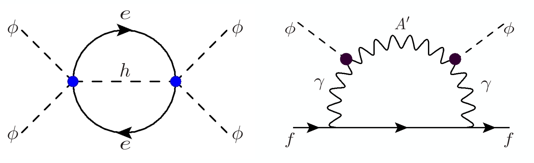
In addition to the flatness of the potential, our model also has the property that it is the electron density, not the nucleon density, that controls $\langle\phi\rangle$. This property is not necessary, and we could repeat the whole analysis for the nucleon case. For simplicity, however, we require that the electron density plays the dominant role. Starting from our tree-level Lagrangian (1), the operator $\bar{f}f\phi^{2}$ for fermion $f$ is induced at 1-loop from diagrams like Fig. 3 right (each $\gamma$ can also be a $Z$). This is given by

where $m_{f}$ and $Q_{f}$ are the mass and electric charge of fermion $f$. When $f$ is a light quark $q=u$, $d$, or $s$, the contribution from the QCD condensate, $m_{q}\langle\bar{q}q\rangle\sim m_{\pi}^{2}f_{\pi}^{2}$, is absorbed in $\mu_{\phi}^{2}$, and the contributions from nucleons can be estimated by replacing $m_{q}\bar{q}q$ by $m_{N}\bar{N}N$ for nucleon $N$. Since $(\alpha_{\rm EM}/\pi)m_{N}/m_{e}\sim 4$, the requirement that the $m_{e}\bar{e}e/\Lambda^{2}$ operator should control $\langle\phi\rangle$ amounts to $\Lambda^{\prime}\gtrsim$ a few$\times\Lambda$, which is already stronger than the condition (16), but to be conservative we impose (shown by the dashed brown line in Fig. 2)

Although this is not strictly necessary as we stated above, this and the bound (20) provides the strongest conditions on the self-consistency of our analysis:

Other potential constraints we checked such as top loop contributions and a radiatively generated $\phi^{2}H^{\dagger}H$ interaction do not impose additional restrictions on the parameter space. We thus see a large parameter space in which quantum corrections do not destroy the flat potential (as well as the dominant role of the electron density).

We begin by a general discussion that new degrees of freedom that UV-completes the EFT should appear roughly at the TeV scale.

Let $M^{\prime}$ be a representative mass scale of new particles in the UV theory responsible for generating the $\phi B^{\mu\nu}F^{\prime}_{\mu\nu}$ operator of the EFT. To generate this operator, the UV theory must contain an interaction linear in $\phi$. Let $y^{\prime}$ be the dimensionless coupling constant of that interaction (measured in units of $M^{\prime}$ if it is dimensionful). Then, roughly, we have

where $g^{\prime}$ and $g_{Y}$ are the U(1)${}_{A^{\prime}}$ and U(1)_Y gauge couplings, respectively, and we have imagined a typical 1-loop factor, $(\text{several})/16\pi^{2}$. (We will later see why it must be at 1-loop.) On the other hand, using the same $y^{\prime}$ vertex 4 times, we also generate a correction to the $\phi^{4}$ operator. In order to avoid fine tuning in $\lambda_{\phi}$ upon matching the UV theory to the EFT, we must roughly impose

Since we know that $\lambda_{\phi}$ is extremely tiny, this shows that $y^{\prime}$ must also be very small. Then, in the relation (24), we see that $M$ can be at quite a low scale despite the fact that $\Lambda^{\prime}$ is very high. To proceed more concretely, we eliminate $\lambda_{\phi}$ in the condition (25) by using the relation (8) with $\epsilon=2.5\times 10^{-13}$ and $n_{\rm c}=4\times 10^{3}\>{\rm keV}$. This gives

Applying this inequality to the matching relation (24), we get

where, from Fig. 2, the maximum possible value of $\Lambda^{\prime}/\Lambda$ is roughly $O(10^{4})$ in a large portion of the allowed region.

Let us do similar general estimates for the UV completion of the electron density dependent operator in (3). Let $M$ be a representative mass scale of new particles responsible for generating the density dependent operator, and $y$ be a representative size of the couplings of $\phi$ to those particles, defined such that each $\phi$ comes with one $y$ (that is, if the interaction is $\propto\phi^{n}$, its coefficient is $\propto y^{n}$ by definition.) Then, upon integrating out the new particles at $M$, we have

where $c$ represents all other coupling constants and numerical factors in the diagram and, if not at tree level, loop factors. As we estimated above for $y^{\prime}$, avoiding fine tuning in $\lambda_{\phi}$ roughly requires $y\lesssim O(10^{2})\>{\rm GeV}/\sqrt{\Lambda\Lambda^{\prime}}$. Using this with the matching condition (28), we get

Both (27) and (29) point to a sub TeV scale for $M^{\prime}$ and $M$, provided that $g^{\prime}\sim c\sim O(1)$.

The existence of new particles with roughly sub-TeV masses is a prediction implied by the allowed region of the EFT parameters. Eq. (27) tells us that we must have $g^{\prime}\sim O(1)$ in order for the new particles at $M^{\prime}$ not to have already been experimentally excluded, since they carry hypercharge to generate the $\phi B^{\mu\nu}F^{\prime}_{\mu\nu}$ operator. Therefore, it is guaranteed that we will have new electrically charged particles with sub-TeV masses with $O(1)$ couplings to the dark photon. Moreover, the $\phi B^{\mu\nu}F^{\prime}_{\mu\nu}$ operator should not be generated at a higher loop order than one as that would lower $M^{\prime}$ too much. This means the new particles at $M^{\prime}$ must couple to $\phi$ at tree level, albeit with tiny couplings. Similarly, in order for the new particles at $M$ not to be too light, they must generate the density dependent operator at tree level with all couplings except $y$ being $O(1)$ so that $c\sim O(1)$.

Therefore, from the general estimates, we already see the opportunity to experimentally probe our scenario further with a window into the dark sector for laboratory experiments. We also see that the structure of any explicit model of the UV completion is very constrained.

Now that it is testable experimentally, it is worth building an explicit example of the UV completion. Conceptually, we must also address the UV origin of the $Z_{2}$ symmetry (2), which we call $Z_{2}^{A^{\prime}}$, so let us begin with this. Since $A^{\prime}$ is odd under $Z_{2}^{A^{\prime}}$ while all SM gauge fields are even, $Z_{2}^{A^{\prime}}$ must act as charge conjugation for U(1)${}_{A^{\prime}}$ while it must not for the SM gauge group. The simplest possibility, therefore, is to introduce two new heavy particles $\psi_{1,2}$ exchanged by $Z_{2}^{A^{\prime}}$ with opposite U(1)${}_{A^{\prime}}$ charges and the same SM charges. The SM charges must at least include a nonzero hypercharge to generate the $\phi B^{\mu\nu}F^{\prime}_{\mu\nu}$ operator. For simplicity and definiteness, we take $\psi_{1,2}$ to be Dirac fermions with $M^{\prime}$, $Y_{\psi}$, and $\pm g^{\prime}$ being their common mass, hypercharge, and the opposite U(1)${}_{A^{\prime}}$ charges, respectively. For $\phi$, we have $\phi\to-\phi$ under $Z_{2}^{A^{\prime}}$ in the UV just as in the EFT.

Now the UV degrees of freedom and symmetries have been fixed.²² 2 If cosmological domain walls from the $Z_{2}^{A^{\prime}}$ breaking become a problem, we can softly break $Z_{2}^{A^{\prime}}$ by introducing a small mass splitting between $\psi_{1}$ and $\psi_{2}$. This will induce a bare kinetic mixing between $B_{\mu\nu}$ and $F^{\prime}_{\mu\nu}$, which must be smaller than the $10^{-15}$ level (see Fig. 1). Gauge symmetries and $Z_{2}^{A^{\prime}}$ allow just one coupling between $\psi_{1,2}$ and $\phi$:

Thus, the new particles $\psi_{1,2}$ couple to $\phi$ at tree level as required by the general analysis above. This is another reason why we need at least two new degrees of freedom to realize $Z_{2}^{A^{\prime}}$. If we just had one $\psi$ and conjugate $\psi$ itself under $Z_{2}^{A^{\prime}}$, we would not be able to couple it to $\phi$.

Accidentally, this UV model can also offer a WIMP DM candidate if $\psi_{1,2}$ contain an electrically neutral state, because the Lagrangian has an accidental U(1)${}_{\psi_{1}}\times$U(1)${}_{\psi_{2}}$ global symmetry, which ensures the neutral state to be stable if it is the lightest.

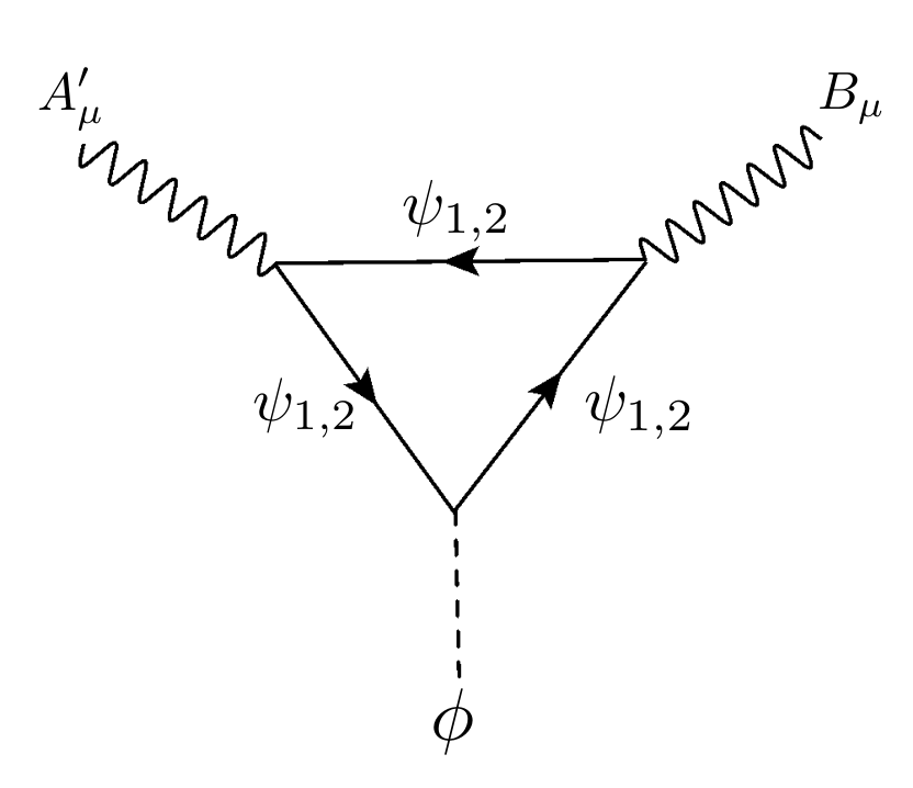
The $\phi B^{\mu\nu}F^{\prime}_{\mu\nu}$ operator is generated at 1-loop from $\psi_{1,2}$ loops (see Fig. 4). We find

Then, following the steps that led to the bounds (27) with more precise numerical coefficients for this model, we find

It should be emphasized that this inequality is still rough as it comes from the condition not to fine-tune $\lambda_{\phi}$ against quantum corrections, which is not a quantitatively sharp criterion. Moreover, the right-hand side above will be enhanced by a factor of $N^{3/4}$ if there are $N$ pairs of $\psi_{1,2}$, which is natural if $\psi_{i}$ forms a multiplet under some other symmetry such as SU(2)_W.

Let us now explicitly UV complete the electron density dependent operator. The aforementioned requirement of generating the operator at tree level via $O(1)$ couplings to the electron and/or Higgs strongly suggests vectorlike leptons with Yukawa couplings to $\phi$. A minimal possibility is to consider two vector-like pairs of leptons, $L_{\rm L,R}$ and $E_{\rm L,R}$, with masses $M_{L}$ and $M_{E}$, respectively. All of these are neutral under U(1)${}_{A^{\prime}}$, and they are all odd under $Z_{2}^{A^{\prime}}$. Writing down all gauge and $Z_{2}^{A^{\prime}}$ invariant renormalizable interactions, we have

where $\ell_{\rm L}$ and $e_{\rm R}$ are the SM lepton fields. Integrating out the vector-like leptons at tree level, we find

Therefore, $c=2y_{E}^{\phantom{*}}$, $y=\sqrt{y_{1}y_{2}^{*}}$, and $M=\sqrt{M_{L}M_{E}}$ in Eq. (28). Upon integrating out $L$ and $E$, corrections to $\lambda_{\phi}$ is given by

up to scheme dependent finite terms. So, our estimate (29) is now refined as

Thus, this can be experimentally probed as well. Unlike the guaranteed existence of new hypercharged particles at $M^{\prime}$, however, the vectorlike leptons may not be a unique possibility. For example, it may be possible that the new particles at $M$ carry no SM charges, e.g., via some kind of a Higgs portal. Also, a viable range of $\Lambda^{\prime}/\Lambda$ is small in the simple example construction above, which could become larger for a complicated model with multiple hierarchical scales and couplings. But such model building exercises are beyond the scope of our present work.

The simple UV model above offers rich experimental probes. First, electroweak/Higgs precision tests place severe constraints on a vector-like lepton Ellis:2014dza, which tends to push the mass beyond the LHC reach Kumar:2015tna; Aaboud:2019trc; Khachatryan:2016sfv. However, if the flavor/CP structures of the Yukawa couplings (33) are generic, the vector-like-lepton sector can be indirectly tested through lepton flavor violation, such as $\mu\to e\gamma$ and $\mu\to eee$ Papa:2020umc, as well as the electric dipole moment of the electron Andreev:2018ayy.

On the other hand, $\psi_{i}$ ($i=1,2$) can be produced at the LHC because the mass scale is expected to be a few hundred GeV as in (32). They can be constrained by searches for heavy charged states Aaboud:2019trc; Khachatryan:2016sfv. The bound can be relaxed if $\psi_{i}$ is a weak multiplet containing a neutral state $\psi_{i}^{0}$ (e.g., a weak doublet (triplet) with $Y_{\psi}=1/2$ ($Y_{\psi}=1$)), which will allow weak decays of the charged states, e.g., $\psi_{i}^{\pm}\to\psi_{i}^{0}\pi^{\pm}$. The neutral states $\psi_{i}^{0}$ can be a WIMP dark matter candidate as they are stable thanks to the accidental U(1)${}_{\psi_{1}}\times$U(1)${}_{\psi_{2}}$ symmetry mentioned below (30). In this case, searches for disappearing tracks will be relevant (e.g. Sirunyan:2020pjd; ATL-PHYS-PUB-2019-011). Detailed phenomenologies are UV model specific and beyond the scope of the present paper.

The most obvious alternative to our dark photon scenario of Sec. II would be the following. In Fig. 1, instead of going down by turning off $\epsilon$ in dense stars, going far to the left by turning off $m_{A^{\prime}}$ in dense stars could also evade the HB/RG bounds. It is straightforward to modify the Lagrangian (1) to realize this alternative. We just need to do two replacements: (i) replace the $\phi B^{\mu\nu}F^{\prime}_{\mu\nu}$ interaction by a bare kinetic mixing term $\epsilon B^{\mu\nu}F^{\prime}_{\mu\nu}$ with a fixed mixing parameter $\epsilon=2.5\times 10^{-13}$, and (ii) replace the real scalar $\phi$ by a complex scalar $\Phi$ charged under U(1)${}_{A^{\prime}}$, and delete the Stückelberg mass term for $A^{\prime}$. Then, denoting the U(1)${}_{A^{\prime}}$ gauge coupling by $g^{\prime}$, we would have $m_{A^{\prime}}=g^{\prime}\langle\Phi\rangle=2.3\>{\rm keV}$ in the vacuum/sun while $m_{A^{\prime}}=0$ in HB/RG stars. This would be a simpler theory as it introduces only one non-renormalizable operator, $m_{e}\bar{e}e|\Phi|^{2}/\Lambda^{2}$, rather than two.

It does not work, however. Essentially, the problem is that, unlike $\phi$ in the model of Sec. II, $\Phi$ here is charged under U(1)${}_{A^{\prime}}$. The CW potential from $A^{\prime}$ loop can then more directly impact the flatness of the $\Phi$ potential here than in the $\phi$ case. If we decrease $g^{\prime}$ to mitigate the impact, we would have to increase $\langle\Phi\rangle$ to keep $m_{A^{\prime}}$ fixed in the vacuum/sun, which, however, would require an even more flat potential. While the model still passes all 1-loop tests, it does not survive through the 2-loop diagrams discussed around Eq. (19). Here, Eq. (19) should be adapted as follows. The scale $\Lambda$ can be eliminated in favor of $v_{0}$ and $\lambda_{\phi}$ via $\lambda_{\phi}v_{0}^{2}\sim m_{e}n_{\rm c}/\Lambda^{2}$, where $v_{0}$ can be further expressed as $v_{0}=m_{A^{\prime}}/g^{\prime}$. The modified Eq. (19) now roughly reads $g^{\prime 4}/\lambda_{\phi}\gtrsim(m_{h}m_{A^{\prime}}^{2}/n_{\rm c})^{2}/(16\pi^{4})\sim 10^{7}$ for $m_{A^{\prime}}\sim 2\>{\rm keV}$ and $n_{\rm c}\sim 10^{3}\>{\rm keV}^{3}$. But this contradicts with the condition $g^{\prime 4}/\lambda_{\phi}\lesssim 1$ to ensure the 1-loop CW potential from $A^{\prime}$ loop not to destroy the flat potential.

The same reason also excludes yet another dark photon scenario in which $m_{A^{\prime}}$ increases in dense stars instead of decreasing. This is the same model as above except that the sign of the $\bar{e}e|\Phi|^{2}/\Lambda$ term is flipped so that U(1)${}_{A^{\prime}}$ is more broken in denser stars than in the vacuum/sun. Since the estimates above never relied on the sign of this term, this alternative is also unattainable due to too large quantum corrections. We thus conclude that, at least among the simplest dark photon models, our scenario of Sec. II seems the only viable option.

We now consider the case when an ALP gives the XENON1T signal instead of a dark photon. In this case, we have two directions for utilizing the density dependence: suppressing ALP couplings or increasing the ALP mass in dense stars.

Let us begin by the idea of suppressing ALP couplings. In the “chameleon-like” ALP model of Ref. Bloch:2020uzh, there is an operator, $c_{ee}m_{e}\bar{e}eXS/M^{2}$, where $X$ and $S$ are respectively real and complex scalars, both of them being odd under a $Z_{2}$ symmetry. The ALP, $a$, comes from $S\sim(f_{a}+s)\,{\rm e}^{{\rm i}a/f_{a}}$. The potential $V(X)$ is identical to our potential $V(\phi)$ in (3) with the replacements of $\phi$ and $m_{e}\bar{e}e/\Lambda^{2}$ by $X$ and $\rho/M^{2}$, respectively, where $\rho$ is the energy density as opposed to the number density. Thus, in dense stars $\langle X\rangle$ vanishes and eliminates the stellar cooling problem due to ALP production.

Unfortunately, as it is already discussed in Ref. Bloch:2020uzh, the flatness of the potential suffers from too large quantum corrections. In addition, since $\rho$ appears in a quantum field theory Lagrangian, we interpret it as arising as the expectation value of a dynamical operator such as $m_{e}\bar{e}e$, $m_{N}\bar{N}N$ or ${\rm tr}[G_{\mu\nu}G^{\mu\nu}]$, where $N$ and $G$ are a nucleon and the gluon field, respectively. Then, there are additional loops from, e.g., a gluon loop or two-loop diagrams as in Fig. 3 left. We also find that the $c_{ee}$ operator generates a tadpole term of $X$ in dense stars proportional to $n_{e}$ which prevents $\langle X\rangle$ from vanishing. These effects could lead to even stronger constraints on the potential.

We now switch to the idea of increasing the ALP mass. In Ref. DeRocco:2020xdt, the ALP mass increases in dense stars as $\langle\phi\rangle$ and its production is kinematically forbidden when the mass becomes heavier than the core temperature of the star. The ALP is the “pion” of a dark QCD, where the dark quark masses are proportional to $\langle\phi\rangle^{2}$ via a see-saw with a heavy fermion. A nonzero $\langle\phi\rangle$ arises from a tadpole due to a Yukawa interaction $\phi\bar{N}N$ when the nucleon density $\bar{N}N$ is turned on.

Ref. DeRocco:2020xdt already mentions fine tuning issues in some parameters in the dark sector. Here, to relate to our earlier discussions, let us look at 1-loop quantum corrections to the $\phi$ potential. In particular, the see-saw requires Yukawa couplings of $\phi$ to a light dark quark and a heavy dark quark, which then contribute to the 1-loop CW potential from dark quark loops, where the coefficient of $\phi^{2n}$ is roughly given by $y^{2n}M^{4-2n}/16\pi^{2}$. Requiring the generated $\phi^{2n}$ term to be smaller than the tree-level $\lambda\phi^{4}$ for $\phi\sim\langle\phi\rangle$, we have $y^{2n}(\langle\phi\rangle/M)^{2n-4}/16\pi^{2}\lesssim\lambda$. In the benchmark model of Ref. DeRocco:2020xdt, we have $\lambda=10^{-78}$, $y=\sqrt{g_{1}g_{2}}=3\times 10^{-11}$, $M=30\,{\rm TeV}$, and $\langle\phi\rangle\simeq 3\times 10^{12}\,m_{a}$ with $m_{a}\simeq 7\>{\rm MeV}$ in white dwarfs. With these values, the potential needs to be fine-tuned up to and including $\phi^{10}$.

As our final example, we consider a scenario where the ALP coupling to the electron is proportional to $1/\langle\phi\rangle$, where $\langle\phi\rangle$ increase in dense stars to suppress the ALP production. This can be realized in a DFSZ-like model of the axion Dine:1981rt; Zhitnitsky:1980tq where $\langle\phi\rangle$ breaks the Pecci-Quinn (PQ) symmetry in a density dependent way as in (3) but with the sign of the $\Lambda^{2}$ term being flipped. Provided that $\langle\phi\rangle$ in the vacuum, $v_{0}$, is much larger than the electroweak symmetry breaking scale, the coupling of the axion to the electron is given by $(m_{e}/v_{0})\,a\bar{e}\gamma_{5}e$. Then, from the value of $g_{aee}$ in Ref. Aprile:2020tmw, we get $v_{0}\sim 10^{9}\,{\rm GeV}$.

Now, the cutoff $\Lambda$ of the effective theory provides the maximum possible value of $\langle\phi\rangle$ in a dense environment. The validity of the theory in white dwarfs, where the electron density is $10^{4}$ higher than in the sun, requires $\Lambda\gtrsim 10^{2}\,v_{0}\sim 10^{11}\,{\rm GeV}$. Such large $\Lambda$ forces $\mu_{\phi}\lesssim 10^{-11}\,{\rm eV}$. The large hierarchy between $m_{\phi}$ and $v_{0}$ requires a tiny quartic coupling $\lambda_{\phi}\sim\mu_{\phi}^{2}/v_{0}^{2}\lesssim 10^{-58}$. But the theory needs an interaction of the form $c\phi^{2}H_{1}H_{2}$ to identify the global U(1) carried by $\phi$ as the U(1)${}_{\text{PQ}}$ carried by the two Higgs doublets (and, therefore, the SM fermions). This operator radiatively corrects $\lambda_{\phi}$, which is roughly $c^{2}/16\pi^{2}$. But one of the CP-odd scalars, $A$, has a mass $m_{A}\sim\sqrt{c}v_{0}$. Requiring $m_{A}\gtrsim 100\>{\rm GeV}$, we have $c\gtrsim 10^{-14}$, but this implies the above correction to $\lambda_{\phi}$ is at least $\sim 10^{-30}$, which is $\gg 10^{-58}$. Thus, again, the model suffers from too large quantum corrections.

To conclude, it appears to be generic that an extremely flat potential is needed to explain the XENON1T excess while evading the stellar cooling problems in denser stars by a density-dependent vev of a scalar field. What we have seen in the examples above is that it is not easy to maintain the flatness of the potential at quantum level. Therefore, it is quite nontrivial that our dark photon model has a large region in the parameter space where the potential receives no large quantum corrections (except for the mass terms, of course).

References

- (1) XENON Collaboration, E. Aprile et al., “Observation of Excess Electronic Recoil Events in XENON1T,” arXiv:2006.09721 [hep-ex].
- (2) H. An, M. Pospelov, J. Pradler, and A. Ritz, “Direct Detection Constraints on Dark Photon Dark Matter,” Phys. Lett. B 747 (2015) 331–338, arXiv:1412.8378 [hep-ph].
- (3) G. Raffelt, Stars as laboratories for fundamental physics: The astrophysics of neutrinos, axions, and other weakly interacting particles. 5, 1996.
- (4) J. Redondo, “Helioscope Bounds on Hidden Sector Photons,” JCAP 07 (2008) 008, arXiv:0801.1527 [hep-ph].
- (5) H. An, M. Pospelov, and J. Pradler, “New stellar constraints on dark photons,” Phys. Lett. B 725 (2013) 190–195, arXiv:1302.3884 [hep-ph].
- (6) M. Giannotti, I. Irastorza, J. Redondo, and A. Ringwald, “Cool WISPs for stellar cooling excesses,” JCAP 05 (2016) 057, arXiv:1512.08108 [astro-ph.HE].
- (7) E. Hardy and R. Lasenby, “Stellar cooling bounds on new light particles: plasma mixing effects,” JHEP 02 (2017) 033, arXiv:1611.05852 [hep-ph].
- (8) M. Giannotti, I. G. Irastorza, J. Redondo, A. Ringwald, and K. Saikawa, “Stellar Recipes for Axion Hunters,” JCAP 10 (2017) 010, arXiv:1708.02111 [hep-ph].
- (9) H. An, M. Pospelov, J. Pradler, and A. Ritz, “New limits on dark photons from solar emission and keV scale dark matter,” arXiv:2006.13929 [hep-ph].
- (10) C. Gao, J. Liu, L.-T. Wang, X.-P. Wang, W. Xue, and Y.-M. Zhong, “Re-examining the Solar Axion Explanation for the XENON1T Excess,” arXiv:2006.14598 [hep-ph].
- (11) L. Di Luzio, M. Fedele, M. Giannotti, F. Mescia, and E. Nardi, “Solar axions cannot explain the XENON1T excess,” arXiv:2006.12487 [hep-ph].
- (12) I. M. Bloch, A. Caputo, R. Essig, D. Redigolo, M. Sholapurkar, and T. Volansky, “Exploring New Physics with O(keV) Electron Recoils in Direct Detection Experiments,” arXiv:2006.14521 [hep-ph].
- (13) R. Budnik, H. Kim, O. Matsedonskyi, G. Perez, and Y. Soreq, “Probing the relaxed relaxion and Higgs-portal with S1 & S2,” arXiv:2006.14568 [hep-ph].
- (14) P. Athron et al., “Global fits of axion-like particles to XENON1T and astrophysical data,” arXiv:2007.05517 [astro-ph.CO].
- (15) D. McKeen, M. Pospelov, and N. Raj, “Hydrogen portal to exotic radioactivity,” arXiv:2006.15140 [hep-ph].
- (16) W. DeRocco, P. W. Graham, and S. Rajendran, “Exploring the robustness of stellar cooling constraints on light particles,” arXiv:2006.15112 [hep-ph].
- (17) R. Budnik, O. Davidi, H. Kim, G. Perez, and N. Priel, “Searching for a solar relaxion or scalar particle with XENON1T and LUX,” Phys. Rev. D 100 no. 9, (2019) 095021, arXiv:1909.02568 [hep-ph].
- (18) M. B. Wise and Y. Zhang, “Lepton Flavorful Fifth Force and Depth-dependent Neutrino Matter Interactions,” JHEP 06 (2018) 053, arXiv:1803.00591 [hep-ph].
- (19) D. Kapner, T. Cook, E. Adelberger, J. Gundlach, B. R. Heckel, C. Hoyle, and H. Swanson, “Tests of the gravitational inverse-square law below the dark-energy length scale,” Phys. Rev. Lett. 98 (2007) 021101, arXiv:hep-ph/0611184.
- (20) E. Salumbides, W. Ubachs, and V. Korobov, “Bounds on fifth forces at the sub-Angstrom length scale,” J. Molec. Spectrosc. 300 (2014) 65, arXiv:1308.1711 [hep-ph].
- (21) S. Schlamminger, K.-Y. Choi, T. Wagner, J. Gundlach, and E. Adelberger, “Test of the equivalence principle using a rotating torsion balance,” Phys. Rev. Lett. 100 (2008) 041101, arXiv:0712.0607 [gr-qc].
- (22) A. Arvanitaki, M. Baryakhtar, and X. Huang, “Discovering the QCD Axion with Black Holes and Gravitational Waves,” Phys. Rev. D 91 no. 8, (2015) 084011, arXiv:1411.2263 [hep-ph].
- (23) S. A. Ellis, R. M. Godbole, S. Gopalakrishna, and J. D. Wells, “Survey of vector-like fermion extensions of the Standard Model and their phenomenological implications,” JHEP 09 (2014) 130, arXiv:1404.4398 [hep-ph].
- (24) N. Kumar and S. P. Martin, “Vectorlike Leptons at the Large Hadron Collider,” Phys. Rev. D 92 no. 11, (2015) 115018, arXiv:1510.03456 [hep-ph].
- (25) ATLAS Collaboration, M. Aaboud et al., “Search for heavy charged long-lived particles in the ATLAS detector in 36.1 fb-1 of proton-proton collision data at TeV,” Phys. Rev. D 99 no. 9, (2019) 092007, arXiv:1902.01636 [hep-ex].
- (26) CMS Collaboration, V. Khachatryan et al., “Search for long-lived charged particles in proton-proton collisions at 13 TeV,” Phys. Rev. D 94 no. 11, (2016) 112004, arXiv:1609.08382 [hep-ex].
- (27) MEG II, Mu3e Collaboration, A. Papa, “Towards a new generation of Charged Lepton Flavour Violation searches at the Paul Scherrer Institut: The MEG upgrade and the Mu3e experiment,” EPJ Web Conf. 234 (2020) 01011.
- (28) ACME Collaboration, V. Andreev et al., “Improved limit on the electric dipole moment of the electron,” Nature 562 no. 7727, (2018) 355–360.
- (29) CMS Collaboration, A. M. Sirunyan et al., “Search for disappearing tracks in proton-proton collisions at 13 TeV,” Phys. Lett. B 806 (2020) 135502, arXiv:2004.05153 [hep-ex].
- (30) ATLAS Collaboration Collaboration, “Performance of tracking and vertexing techniques for a disappearing track plus soft track signature with the ATLAS detector,” Tech. Rep. ATL-PHYS-PUB-2019-011, CERN, Geneva, Mar, 2019. https://cds.cern.ch/record/2669015.
- (31) M. Dine, W. Fischler, and M. Srednicki, “A Simple Solution to the Strong CP Problem with a Harmless Axion,” Phys. Lett. 104B (1981) 199–202.
- (32) A. R. Zhitnitsky, “On Possible Suppression of the Axion Hadron Interactions. (In Russian),” Sov. J. Nucl. Phys. 31 (1980) 260. [Yad. Fiz.31,497(1980)].
- (33) R. Lasenby and K. Van Tilburg, “Dark Photons in the Solar Basin,” arXiv:2008.08594 [hep-ph].