跳到论文正文
W Papers独立论文阅读器 arXiv:2008.10554 论文正文 计算阅读时间 · 0%
引用这篇论文根据当前论文元数据生成,正式投稿前建议核对。


License: arXiv.org perpetual non-exclusive license
arXiv:2008.10554v1 [math.NA] 24 Aug 2020

Eigenvalues and Eigenvectors of Tau Matrices
with Applications to Markov Processes and EconomicsThanks: Correspondence to: Carlo Garoni (garoni@mat.uniroma2.it).

Sven-Erik Ekström Affiliation: [-2pt] Department of Information Technology, Division of Scientific Computing, Uppsala University, Sweden Affiliation: [-2pt] Faculty of Mathematics and Natural Sciences, Bergische Universität Wuppertal, Germany Affiliation: [7pt] Carlo Garoni Affiliation: [-2pt] Department of Mathematics, University of Rome Tor Vergata, Italy Affiliation: [7pt] Adam Jozefiak Affiliation: [-2pt] Department of Computer Science, University of British Columbia, Canada Affiliation: [7pt] Jesse Perla Affiliation: [-2pt] Vancouver School of Economics, University of British Columbia, Canada
Abstract

In the context of matrix displacement decomposition, Bozzo and Di Fiore introduced the so-called τε,φ\tau_{\varepsilon,\varphi} algebra, a generalization of the more known τ\tau algebra originally proposed by Bini and Capovani. We study the properties of eigenvalues and eigenvectors of the generator Tn,ε,φT_{n,\varepsilon,\varphi} of the τε,φ\tau_{\varepsilon,\varphi} algebra. In particular, we derive the asymptotics for the outliers of Tn,ε,φT_{n,\varepsilon,\varphi} and the associated eigenvectors; we obtain equations for the eigenvalues of Tn,ε,φT_{n,\varepsilon,\varphi}, which provide also the eigenvectors of Tn,ε,φT_{n,\varepsilon,\varphi}; and we compute the full eigendecomposition of Tn,ε,φT_{n,\varepsilon,\varphi} in the specific case ε​φ=1\varepsilon\varphi=1. We also present applications of our results in the context of queuing models, random walks, and diffusion processes, with a special attention to their implications in the study of wealth/income inequality and portfolio dynamics.

Keywords: eigenvalues and eigenvectors, tau matrices, queuing models, random walks, diffusion processes, wealth and income inequality, portfolio dynamics

2020 MSC: 15A18, 15B05, 60K25, 60G50, 60J60, 91G10

1 Introduction

Consider the n×nn\times n matrix

Tn,ε,φ=[ε1101⋱⋱⋱1011φ],T_{n,\varepsilon,\varphi}=\begin{bmatrix}\varepsilon&1&&&\\ 1&0&1&&\\ &\ddots&\ddots&\ddots&\\ &&1&0&1\\ &&&1&\varphi\end{bmatrix},

where ε,φ∈ℝ\varepsilon,\varphi\in\mathbb{R} are given parameters. For ε,φ∈{0,1,−1}\varepsilon,\varphi\in\{0,1,-1\}, the eigendecomposition of Tn,ε,φT_{n,\varepsilon,\varphi} is already available in the literature. In particular, for (ε,φ)=(0,0)(\varepsilon,\varphi)=(0,0), the matrix Tn,ε,φ=Tn,0,0T_{n,\varepsilon,\varphi}=T_{n,0,0} is the generator of the τ\tau algebra originally introduced by Bini and Capovani [10]; its eigendecomposition, as well as the eigendecomposition of any tridiagonal Toeplitz matrix, has long been known [12, Section 2.2]. For (ε,φ)≠(0,0)(\varepsilon,\varphi)\neq(0,0), the matrix Tn,ε,φT_{n,\varepsilon,\varphi} is the generator of the so-called τε,φ\tau_{\varepsilon,\varphi} algebra introduced by Bozzo and Di Fiore in [13]; its eigendecomposition for (ε,φ)=(1,1)(\varepsilon,\varphi)=(1,1), (−1,−1)(-1,-1), (1,−1)(1,-1), (−1,1)(-1,1) was provided in [13, Section 4]. Finally, for (ε,φ)=(1,0)(\varepsilon,\varphi)=(1,0), (0,1)(0,1), (−1,0)(-1,0), (0,−1)(0,-1)—actually for all ε,φ∈{0,1,−1}\varepsilon,\varphi\in\{0,1,-1\}—the eigendecomposition of Tn,ε,φT_{n,\varepsilon,\varphi} can be derived, e.g., from the results in [15, Appendix 1]; see in particular [15, pp. 394–395].

For all ε,φ∈ℝ\varepsilon,\varphi\in\mathbb{R}, the asymptotic spectral distribution of Tn,ε,φT_{n,\varepsilon,\varphi} in Weyl’s sense can be easily obtained from the theory of generalized locally Toeplitz sequences [19, 20], which immediately yields for Tn,ε,φT_{n,\varepsilon,\varphi} the asymptotic spectral distribution function (or symbol) 2​cos⁡θ2\cos\theta. Precise eigenvalue estimates can also be given on the basis of classical interlacing results [22, Section 4.3] after observing that Tn,ε,φT_{n,\varepsilon,\varphi} is a small-rank perturbation of Tn,0,0T_{n,0,0} and the eigenvalues of Tn,0,0T_{n,0,0} are known. It should be noted, however, that both asymptotic spectral distribution results and interlacing estimates completely ignore the outliers of Tn,ε,φT_{n,\varepsilon,\varphi}, i.e., the eigenvalues lying outside the interval [−2,2][-2,2] (the range of the symbol 2​cos⁡θ2\cos\theta). On the other hand, the outliers, which are determined by the parameters ε,φ\varepsilon,\varphi, are precisely the objects one is interested in when dealing with several noteworthy applications. Such applications include, for example, queuing models and Markov chains/processes [5, 9, 21, 24], where the eigenvector corresponding to the (unique) outlier of (a suitable transform of) Tn,ε,φT_{n,\varepsilon,\varphi} corresponds to the steady-state distribution of the considered chain/process.

In this paper, we study the spectral properties of Tn,ε,φT_{n,\varepsilon,\varphi} and present a few applications in the context of Markov chains/processes, with a special focus on queuing models, random walks, diffusion processes and economics issues. The structure of the paper, including a summary of our contributions, is given below.

  • •

    In Section 2, we study some basic spectral properties of Tn,ε,φT_{n,\varepsilon,\varphi} that will simplify the analysis of later sections.

  • •

    In Section 3, we derive the asymptotics of the outliers of Tn,ε,φT_{n,\varepsilon,\varphi} and the associated eigenvectors. Our main results in this regard are Theorems 3.1–3.3, which are validated through numerical experiments in Tables 3.1–3.3.

  • •

    In Section 4, we derive equations for the eigenvalues of Tn,ε,φT_{n,\varepsilon,\varphi}. For all ε,φ∈ℝ\varepsilon,\varphi\in\mathbb{R} for which these equations can be solved, one obtains not only the eigenvalues but also the eigenvectors of Tn,ε,φT_{n,\varepsilon,\varphi}. Our main results in Section 4 are Theorems 4.1–4.5.

  • •

    In Section 5, we solve the equations obtained in Section 4 for specific values of ε,φ\varepsilon,\varphi. In particular, we show how it is possible to re-obtain through our equations the eigendecomposition of Tn,ε,φT_{n,\varepsilon,\varphi} for ε,φ∈{0,1,−1}\varepsilon,\varphi\in\{0,1,-1\}; and we address the new case ε​φ=1\varepsilon\varphi=1, which is the case of interest for the applications presented in Section 6.

  • •

    In Section 6, we present a few applications in the context of Markov chains/processes, with a special focus on queuing models, random walks in a multidimensional lattice, multidimensional reflected diffusion processes and economics issues. In particular, we investigate the implications of our results within a model for wealth/income inequality and portfolio dynamics with an arbitrary number of assets: we provide analytical formulas for the steady-state (stationary) distribution of the underlying stochastic process (a multidimensional reflected diffusion process), we compute the convergence speed towards the steady state, and we also derive closed-form expressions for relevant moments of the stationary distribution such as the average wealth and the wealth variance.

  • •

    In Section 7, we draw conclusions and outline possible future lines of research.

2 Basic Properties of the Eigenvalues and Eigenvectors of 𝑻𝒏,𝜺,𝝋\boldsymbol{T_{n,\varepsilon,\varphi}}

In this section, we collect some basic properties of the eigenvalues and eigenvectors of Tn,ε,φT_{n,\varepsilon,\varphi} which will allow us to tackle the analysis of the next sections with useful a priori knowledge. Throughout this paper, the eigenvalues of Tn,ε,φT_{n,\varepsilon,\varphi} which do not belong to the interval [−2,2][-2,2] are referred to as outliers. We denote by 𝐞1,…,𝐞n{\mathbf{e}}_{1},\ldots,{\mathbf{e}}_{n} the vectors of the canonical basis of ℝn\mathbb{R}^{n}, and by EnE_{n} the symmetric permutation matrix (flip matrix) whose rows are those of the identity matrix InI_{n} in reverse order:

En=[1⋰1].E_{n}=\begin{bmatrix}&&1\\ &\iddots&\\ 1&&\end{bmatrix}.
Theorem 2.1.

The following properties hold.

  1. 1.

    Tn,φ,ε=En​Tn,ε,φ​EnT_{n,\varphi,\varepsilon}=E_{n}T_{n,\varepsilon,\varphi}E_{n}. It follows that (λ,𝐮)(\lambda,{\mathbf{u}}) is an eigenpair of Tn,ε,φT_{n,\varepsilon,\varphi} if and only if (λ,En​𝐮)(\lambda,E_{n}{\mathbf{u}}) is an eigenpair of Tn,φ,εT_{n,\varphi,\varepsilon}.

  2. 2.

    If ε≠0\varepsilon\neq 0 and

    𝐯n=[ε−i+1]i=1n=[1ε−1ε−n+1]{\mathbf{v}}_{n}=[\varepsilon^{-i+1}]_{i=1}^{n}=\begin{bmatrix}1\\ \varepsilon^{-1}\\ \vdots\\ \varepsilon^{-n+1}\end{bmatrix}

    then Tn,ε,φ​𝐯n−(ε+ε−1)​𝐯n=ε−n​(ε​φ−1)​𝐞nT_{n,\varepsilon,\varphi}{\mathbf{v}}_{n}-(\varepsilon+\varepsilon^{-1}){\mathbf{v}}_{n}=\varepsilon^{-n}(\varepsilon\varphi-1){\mathbf{e}}_{n}. Similarly, if φ≠0\varphi\neq 0 and

    𝐰n=[φ−n+i]i=1n=[φ−n+1φ−11]{\mathbf{w}}_{n}=[\varphi^{-n+i}]_{i=1}^{n}=\begin{bmatrix}\varphi^{-n+1}\\ \vdots\\ \varphi^{-1}\\ 1\end{bmatrix}

    then Tn,ε,φ​𝐰n−(φ+φ−1)​𝐰n=φ−n​(ε​φ−1)​𝐞1T_{n,\varepsilon,\varphi}{\mathbf{w}}_{n}-(\varphi+\varphi^{-1}){\mathbf{w}}_{n}=\varphi^{-n}(\varepsilon\varphi-1){\mathbf{e}}_{1}.

  3. 3.

    Tn,ε,φT_{n,\varepsilon,\varphi} has nn real distinct eigenvalues.

  4. 4.

    If |ε|,|φ|≤1|\varepsilon|,|\varphi|\leq 1 then all the eigenvalues of Tn,ε,φT_{n,\varepsilon,\varphi} belong to [−2,2][-2,2].

  5. 5.

    If |ε|≤1,|φ|>1|\varepsilon|\leq 1,\>|\varphi|>1 or |ε|>1,|φ|≤1|\varepsilon|>1,\>|\varphi|\leq 1 then all the eigenvalues of Tn,ε,φT_{n,\varepsilon,\varphi} belong to [−2,2][-2,2] except for at most 11 outlier.

  6. 6.

    If |ε|,|φ|>1|\varepsilon|,|\varphi|>1 then all the eigenvalues of Tn,ε,φT_{n,\varepsilon,\varphi} belong to [−2,2][-2,2] except for at most 22 outliers.

  7. 7.

    If |ε|<1|\varepsilon|<1 or |φ|<1|\varphi|<1 then both 22 and −2-2 are not eigenvalues of Tn,ε,φT_{n,\varepsilon,\varphi}.

Proof.

1. It follows from direct computation.

2. It follows from direct computation.

3. Tn,ε,φT_{n,\varepsilon,\varphi} is nonderogatory just like any Hessenberg matrix with nonzero subdiagonal entries [22, p. 82]. Since Tn,ε,φT_{n,\varepsilon,\varphi} is also real and symmetric (hence diagonalizable), we infer that Tn,ε,φT_{n,\varepsilon,\varphi} has nn real distinct eigenvalues.

4. The result follows immediately from Gershgorin’s theorem [22, Theorem 6.1.1].

5. We prove the statement in the case where |ε|≤1|\varepsilon|\leq 1 and |φ|>1|\varphi|>1 (the proof in the other case is identical). Write

Tn,ε,φ=Tn,ε,0+φ​𝐞n​𝐞n⊤.T_{n,\varepsilon,\varphi}=T_{n,\varepsilon,0}+\varphi\,{\mathbf{e}}_{n}{\mathbf{e}}_{n}^{\top}.

All the eigenvalues of Tn,ε,0T_{n,\varepsilon,0} belong to [−2,2][-2,2] by Gershgorin’s theorem. Since the unique nonzero eigenvalue of the matrix φ​𝐞n​𝐞n⊤\varphi\,{\mathbf{e}}_{n}{\mathbf{e}}_{n}^{\top} is φ\varphi, it follows from a classical interlacing theorem [22, Corollary 4.3.3] that n−1n-1 eigenvalues of Tn,ε,φT_{n,\varepsilon,\varphi} belong to [−2,2][-2,2].

6. Write

Tn,ε,φ=Tn,0,0+ε​𝐞1​𝐞1⊤+φ​𝐞n​𝐞n⊤.T_{n,\varepsilon,\varphi}=T_{n,0,0}+\varepsilon\,{\mathbf{e}}_{1}{\mathbf{e}}_{1}^{\top}+\varphi\,{\mathbf{e}}_{n}{\mathbf{e}}_{n}^{\top}.

All the eigenvalues of Tn,0,0T_{n,0,0} belong to [−2,2][-2,2] by Gershgorin’s theorem. Since the unique nonzero eigenvalues of the matrix ε​𝐞1​𝐞1⊤+φ​𝐞n​𝐞n⊤\varepsilon\,{\mathbf{e}}_{1}{\mathbf{e}}_{1}^{\top}+\varphi\,{\mathbf{e}}_{n}{\mathbf{e}}_{n}^{\top} are ε\varepsilon and φ\varphi, it follows from [22, Corollary 4.3.3] that n−2n-2 eigenvalues of Tn,ε,φT_{n,\varepsilon,\varphi} belong to [−2,2][-2,2].

7. The result follows immediately from the fact that the matrix Tn,ε,φT_{n,\varepsilon,\varphi} is irreducible and from the so-called Gershgorin’s third theorem [11, p. 80]. ∎

3 Asymptotics of the Outliers of 𝑻𝒏,𝜺,𝝋\boldsymbol{T_{n,\varepsilon,\varphi}}

If |ε|>1|\varepsilon|>1 and nn is large enough, property 2 of Theorem 2.1 says that (ε+ε−1,𝐯n)(\varepsilon+\varepsilon^{-1},{\mathbf{v}}_{n}) is substantially an eigenpair of Tn,ε,φT_{n,\varepsilon,\varphi} (it is an exact eigenpair if ε​φ=1\varepsilon\varphi=1). A similar consideration applies to (φ+φ−1,𝐰n)(\varphi+\varphi^{-1},{\mathbf{w}}_{n}). The next theorems formalize this intuition. We remark that, for every x>0x>0,

x+x−1=2​cosh⁡(log⁡x)≥2,x+x^{-1}=2\cosh(\log x)\geq 2,

with equality holding if and only if x=1x=1. In what follows, Λ⁡(X)\Lambda(X) denotes the spectrum of the matrix XX.

Lemma 3.1.

The following properties hold.

  1. 1.

    If |ε|>1|\varepsilon|>1 then there exists an eigenvalue μn\mu_{n} of Tn,ε,φT_{n,\varepsilon,\varphi} such that μn→ε+ε−1\mu_{n}\to\varepsilon+\varepsilon^{-1} as n→∞n\to\infty. Since ε+ε−1>2\varepsilon+\varepsilon^{-1}>2, the eigenvalue μn\mu_{n} is eventually an outlier.

  2. 2.

    If |φ|>1|\varphi|>1 then there exists an eigenvalue νn\nu_{n} of Tn,ε,φT_{n,\varepsilon,\varphi} such that νn→φ+φ−1\nu_{n}\to\varphi+\varphi^{-1} as n→∞n\to\infty. Since φ+φ−1>2\varphi+\varphi^{-1}>2, the eigenvalue νn\nu_{n} is eventually an outlier.

Proof.

1. Let {𝐮1,n,…,𝐮n,n}\{{\mathbf{u}}_{1,n},\ldots,{\mathbf{u}}_{n,n}\} be an orthonormal basis of ℝn\mathbb{R}^{n} formed by eigenvectors of Tn,ε,φT_{n,\varepsilon,\varphi} with corresponding eigenvalues λ1,n,…,λn,n\lambda_{1,n},\ldots,\lambda_{n,n}:

Tn,ε,φ𝐮i,n=λi,n𝐮i,n,i=1,…,n.T_{n,\varepsilon,\varphi}{\mathbf{u}}_{i,n}=\lambda_{i,n}{\mathbf{u}}_{i,n},\qquad i=1,\ldots,n.

Expand the vector 𝐯n=[1,ε−1,…,ε−n+1]⊤{\mathbf{v}}_{n}=[1,\varepsilon^{-1},\ldots,\varepsilon^{-n+1}]^{\top} on this basis:

𝐯n\displaystyle{\mathbf{v}}_{n} =∑i=1nαi,n​𝐮i,n,\displaystyle=\sum_{i=1}^{n}\alpha_{i,n}{\mathbf{u}}_{i,n}, (3.1)
∑i=1nαi,n2\displaystyle\sum_{i=1}^{n}\alpha_{i,n}^{2} =‖𝐯n‖22=1−ε−2​n1−ε−2→11−ε−2.\displaystyle=\|{\mathbf{v}}_{n}\|_{2}^{2}=\frac{1-\varepsilon^{-2n}}{1-\varepsilon^{-2}}\to\frac{1}{1-\varepsilon^{-2}}. (3.2)

The equation Tn,ε,φ​𝐯n−(ε+ε−1)​𝐯n=ε−n​(ε​φ−1)​𝐞nT_{n,\varepsilon,\varphi}{\mathbf{v}}_{n}-(\varepsilon+\varepsilon^{-1}){\mathbf{v}}_{n}=\varepsilon^{-n}(\varepsilon\varphi-1){\mathbf{e}}_{n} in Theorem 2.1 becomes

∑i=1n(λi,n−(ε+ε−1))​αi,n​𝐮i,n=ε−n​(ε​φ−1)​𝐞n.\sum_{i=1}^{n}(\lambda_{i,n}-(\varepsilon+\varepsilon^{-1}))\alpha_{i,n}{\mathbf{u}}_{i,n}=\varepsilon^{-n}(\varepsilon\varphi-1){\mathbf{e}}_{n}. (3.3)

Passing to the norms, we obtain

∑i=1n(λi,n−(ε+ε−1))2​αi,n2=ε−2​n​(ε​φ−1)2→0.\sum_{i=1}^{n}(\lambda_{i,n}-(\varepsilon+\varepsilon^{-1}))^{2}\alpha_{i,n}^{2}=\varepsilon^{-2n}(\varepsilon\varphi-1)^{2}\to 0. (3.4)

If we assume by contradiction that dist⁡(Λ⁡(Tn,ε,φ),ε+ε−1)=mini=1,…,n⁡|λi,n−(ε+ε−1)|↛0{\rm dist}(\Lambda(T_{n,\varepsilon,\varphi}),\varepsilon+\varepsilon^{-1})=\min_{i=1,\ldots,n}|\lambda_{i,n}-(\varepsilon+\varepsilon^{-1})|\not\to 0 as n→∞n\to\infty, then there exists a positive constant cc such that

dist⁡(Λ⁡(Tn,ε,φ),ε+ε−1)≥c{\rm dist}(\Lambda(T_{n,\varepsilon,\varphi}),\varepsilon+\varepsilon^{-1})\geq c

frequently as n→∞n\to\infty, hence

∑i=1n(λi,n−(ε+ε−1))2​αi,n2≥c2​∑i=1nαi,n2=c2​‖𝐯n‖22≥c2\sum_{i=1}^{n}(\lambda_{i,n}-(\varepsilon+\varepsilon^{-1}))^{2}\alpha_{i,n}^{2}\geq c^{2}\sum_{i=1}^{n}\alpha_{i,n}^{2}=c^{2}\|{\mathbf{v}}_{n}\|_{2}^{2}\geq c^{2}

frequently as n→∞n\to\infty, which is a contradiction to (3.4). We conclude that dist⁡(Λ⁡(Tn,ε,φ),ε+ε−1)→0{\rm dist}(\Lambda(T_{n,\varepsilon,\varphi}),\varepsilon+\varepsilon^{-1})\to 0 as n→∞n\to\infty, which is the thesis.

2. It follows from item 1 applied to Tn,φ,εT_{n,\varphi,\varepsilon}, taking into account that Λ⁡(Tn,φ,ε)=Λ⁡(Tn,ε,φ)\Lambda(T_{n,\varphi,\varepsilon})=\Lambda(T_{n,\varepsilon,\varphi}) by Theorem 2.1. ∎

If 𝐱,𝐲∈ℝn{\mathbf{x}},{\mathbf{y}}\in\mathbb{R}^{n}, we set (𝐱,𝐲)=𝐱⊤​𝐲({\mathbf{x}},{\mathbf{y}})={\mathbf{x}}^{\top}{\mathbf{y}}. If 𝐮∈ℝn{\mathbf{u}}\in\mathbb{R}^{n}, we denote by P𝐮P_{{\mathbf{u}}} the orthogonal projector onto the subspace ⟨𝐮⟩\langle{\mathbf{u}}\rangle generated by 𝐮{\mathbf{u}}. In the case where 𝐮≠𝟎{\mathbf{u}}\neq\mathbf{0}, the projector P𝐮P_{\mathbf{u}} is explicitly given by

P𝐮​𝐱=(𝐱,𝐮)(𝐮,𝐮)​𝐮,𝐱∈ℝn.P_{\mathbf{u}}{\mathbf{x}}=\frac{({\mathbf{x}},{\mathbf{u}})}{({\mathbf{u}},{\mathbf{u}})}\,{\mathbf{u}},\qquad{\mathbf{x}}\in\mathbb{R}^{n}.
Table 3.1: Validation of Theorem 3.1 in the case ε=3\varepsilon=3 and φ=1/2\varphi=1/2 where ε+ε−1=3.3¯\varepsilon+\varepsilon^{-1}=3.\overline{3}. For every nn we have denoted by μn\mu_{n} the unique outlier of Tn,ε,φT_{n,\varepsilon,\varphi} and by 𝐱n{\mathbf{x}}_{n} the corresponding normalized eigenvector computed by Julia.
nn outlier μn\mu_{n} |μn−(ε+ε−1)||\mu_{n}-(\varepsilon+\varepsilon^{-1})| ‖𝐱n−P𝐯n​𝐱n‖2\|{\mathbf{x}}_{n}-P_{{\mathbf{v}}_{n}}{\mathbf{x}}_{n}\|_{2}
8 3.3333333663723654  3.3⋅10−8\hphantom{\mu_{n}}\,3.3\cdot 10^{-8}  3.0⋅10−5\hphantom{\|{\mathbf{x}}}\,3.0\cdot 10^{-5}\vphantom{\int^{\Sigma^{1}}}
16 3.3333333333333341  7.7⋅10−16\hphantom{\mu_{n}}\,7.7\cdot 10^{-16}  4.6⋅10−9\hphantom{\|{\mathbf{x}}}\,4.6\cdot 10^{-9}\vphantom{\int^{\Sigma^{1}}}
32 3.3333333333333333  4.1⋅10−31\hphantom{\mu_{n}}\,4.1\cdot 10^{-31}  1.1⋅10−16\hphantom{\|{\mathbf{x}}}\,1.1\cdot 10^{-16}\vphantom{\int^{\Sigma^{1}}}
64 3.3333333333333333  1.2⋅10−61\hphantom{\mu_{n}}\,1.2\cdot 10^{-61}  5.8⋅10−32\hphantom{\|{\mathbf{x}}}\,5.8\cdot 10^{-32}\vphantom{\int^{\Sigma^{1}}}
128 3.3333333333333333  1.0⋅10−122\hphantom{\mu_{n}}\,1.0\cdot 10^{-122}  1.7⋅10−62\hphantom{\|{\mathbf{x}}}\,1.7\cdot 10^{-62}\vphantom{\int^{\Sigma^{1}}}
Theorem 3.1.

Suppose that |ε|>1|\varepsilon|>1 and φ≠ε\varphi\neq\varepsilon. Let (μn,𝐱n)(\mu_{n},{\mathbf{x}}_{n}) be an eigenpair of Tn,ε,φT_{n,\varepsilon,\varphi} such that μn→ε+ε−1\mu_{n}\to\varepsilon+\varepsilon^{-1} as n→∞n\to\infty and ‖𝐱n‖2=1\|{\mathbf{x}}_{n}\|_{2}=1 for all nn. Then, the following properties hold.

  1. 1.

    Eventually, μn\mu_{n} is an outlier of Tn,ε,φT_{n,\varepsilon,\varphi} and any other eigenvalue λn∈Λ⁡(Tn,ε,φ)\lambda_{n}\in\Lambda(T_{n,\varepsilon,\varphi}) satisfies |λn−(ε+ε−1)|≥c|\lambda_{n}-(\varepsilon+\varepsilon^{-1})|\geq c for some positive constant cc independent of nn.

  2. 2.

    ‖𝐱n−P𝐯n​𝐱n‖2→0\|{\mathbf{x}}_{n}-P_{{\mathbf{v}}_{n}}{\mathbf{x}}_{n}\|_{2}\to 0 as n→∞n\to\infty, where 𝐯n=[1,ε−1,…,ε−n+1]⊤{\mathbf{v}}_{n}=[1,\varepsilon^{-1},\ldots,\varepsilon^{-n+1}]^{\top}.

Proof.

1. If |φ|≤1|\varphi|\leq 1 then all eigenvalues of Tn,ε,φT_{n,\varepsilon,\varphi} belong to [−2,2][-2,2] except for at most 1 outlier (by Theorem 2.1). Since μn→ε+ε−1∉[−2,2]\mu_{n}\to\varepsilon+\varepsilon^{-1}\not\in[-2,2], it is clear that μn\mu_{n} coincides eventually with the unique outlier of Tn,ε,φT_{n,\varepsilon,\varphi}. Moreover, any other eigenvalue λn\lambda_{n} of Tn,ε,φT_{n,\varepsilon,\varphi} satisfies the inequality |λn−(ε+ε−1)|≥c|\lambda_{n}-(\varepsilon+\varepsilon^{-1})|\geq c with

c=dist⁡(ε+ε−1,[−2,2]).c={\rm dist}(\varepsilon+\varepsilon^{-1},[-2,2]).

If |φ|>1|\varphi|>1 then all eigenvalues of Tn,ε,φT_{n,\varepsilon,\varphi} belong to [−2,2][-2,2] except for at most 2 outliers (by Theorem 2.1) and there exists an eigenvalue νn\nu_{n} of Tn,ε,φT_{n,\varepsilon,\varphi} such that νn→φ+φ−1∉[−2,2]\nu_{n}\to\varphi+\varphi^{-1}\not\in[-2,2] (by Lemma 3.1). Since μn→ε+ε−1∉[−2,2]\mu_{n}\to\varepsilon+\varepsilon^{-1}\not\in[-2,2] and ε+ε−1≠φ+φ−1\varepsilon+\varepsilon^{-1}\neq\varphi+\varphi^{-1} (because φ≠ε\varphi\neq\varepsilon by assumption), it is clear that, eventually, μn≠νn\mu_{n}\neq\nu_{n} and μn,νn\mu_{n},\nu_{n} are the unique two outliers of Tn,ε,φT_{n,\varepsilon,\varphi}. Moreover, any eigenvalue λn\lambda_{n} of Tn,ε,φT_{n,\varepsilon,\varphi} with λn≠μn\lambda_{n}\neq\mu_{n} satisfies eventually the inequality |λn−(ε+ε−1)|≥c|\lambda_{n}-(\varepsilon+\varepsilon^{-1})|\geq c with

c=dist⁡(ε+ε−1,[−2,2]∪[φ+φ−1−δ,φ+φ−1+δ]),c={\rm dist}(\varepsilon+\varepsilon^{-1},[-2,2]\cup[\varphi+\varphi^{-1}-\delta,\,\varphi+\varphi^{-1}+\delta]),

where δ\delta is a fixed positive constant chosen so that ε+ε−1∉[φ+φ−1−δ,φ+φ−1+δ]\varepsilon+\varepsilon^{-1}\not\in[\varphi+\varphi^{-1}-\delta,\,\varphi+\varphi^{-1}+\delta].

2. Let {𝐮1,n,…,𝐮n,n=𝐱n}\{{\mathbf{u}}_{1,n},\ldots,{\mathbf{u}}_{n,n}={\mathbf{x}}_{n}\} be an orthonormal basis of ℝn\mathbb{R}^{n} formed by eigenvectors of Tn,ε,φT_{n,\varepsilon,\varphi} with corresponding eigenvalues λ1,n,…,λn,n=μn\lambda_{1,n},\ldots,\lambda_{n,n}=\mu_{n}:

Tn,ε,φ𝐮i,n=λi,n𝐮i,n,i=1,…,n.T_{n,\varepsilon,\varphi}{\mathbf{u}}_{i,n}=\lambda_{i,n}{\mathbf{u}}_{i,n},\qquad i=1,\ldots,n.

We expand the vector 𝐯n{\mathbf{v}}_{n} on this basis as in (3.1) and we get (3.2)–(3.4). By item 1, we eventually have

∑i=1n(λi,n−(ε+ε−1))2​αi,n2≥c2​∑i=1n−1αi,n2+(μn−(ε+ε−1))2​αn,n2.\sum_{i=1}^{n}(\lambda_{i,n}-(\varepsilon+\varepsilon^{-1}))^{2}\alpha_{i,n}^{2}\geq c^{2}\sum_{i=1}^{n-1}\alpha_{i,n}^{2}+(\mu_{n}-(\varepsilon+\varepsilon^{-1}))^{2}\alpha_{n,n}^{2}. (3.5)

Hence, by (3.2) and (3.4),

∑i=1n−1αi,n2→0,αn,n2→11−ε−2.\sum_{i=1}^{n-1}\alpha_{i,n}^{2}\to 0,\qquad\alpha_{n,n}^{2}\to\frac{1}{1-\varepsilon^{-2}}. (3.6)

Keeping in mind (3.1), (3.2) and (3.6), we obtain

‖𝐱n−P𝐯n​𝐱n‖22\displaystyle\|{\mathbf{x}}_{n}-P_{{\mathbf{v}}_{n}}{\mathbf{x}}_{n}\|_{2}^{2} =‖𝐮n,n−P𝐯n​𝐮n,n‖22=‖𝐮n,n−(𝐮n,n,𝐯n)(𝐯n,𝐯n)​𝐯n‖22=‖𝐮n,n−αn,n‖𝐯n‖22​∑i=1nαi,n​𝐮i,n‖22\displaystyle=\|{\mathbf{u}}_{n,n}-P_{{\mathbf{v}}_{n}}{\mathbf{u}}_{n,n}\|_{2}^{2}=\left\|{\mathbf{u}}_{n,n}-\frac{({\mathbf{u}}_{n,n},{\mathbf{v}}_{n})}{({\mathbf{v}}_{n},{\mathbf{v}}_{n})}\,{\mathbf{v}}_{n}\right\|_{2}^{2}=\left\|{\mathbf{u}}_{n,n}-\frac{\alpha_{n,n}}{\|{\mathbf{v}}_{n}\|_{2}^{2}}\sum_{i=1}^{n}\alpha_{i,n}{\mathbf{u}}_{i,n}\right\|_{2}^{2}
=‖(1−αn,n2‖𝐯n‖22)​𝐮n,n+αn,n‖𝐯n‖22​∑i=1n−1αi,n​𝐮i,n‖22=(1−αn,n2‖𝐯n‖22)2+αn,n2‖𝐯n‖24​∑i=1n−1αi,n2→0,\displaystyle=\left\|\biggl(1-\frac{\alpha_{n,n}^{2}}{\|{\mathbf{v}}_{n}\|_{2}^{2}}\biggr){\mathbf{u}}_{n,n}+\frac{\alpha_{n,n}}{\|{\mathbf{v}}_{n}\|_{2}^{2}}\sum_{i=1}^{n-1}\alpha_{i,n}{\mathbf{u}}_{i,n}\right\|_{2}^{2}=\biggl(1-\frac{\alpha_{n,n}^{2}}{\|{\mathbf{v}}_{n}\|_{2}^{2}}\biggr)^{2}+\frac{\alpha_{n,n}^{2}}{\|{\mathbf{v}}_{n}\|_{2}^{4}}\sum_{i=1}^{n-1}\alpha_{i,n}^{2}\to 0, (3.7)

which concludes the proof. ∎

The next theorem is completely analogous to Theorem 3.1 and can be proved by the same type of argument or by using the relation between Tn,ε,φT_{n,\varepsilon,\varphi} and Tn,φ,εT_{n,\varphi,\varepsilon} (see Theorem 2.1).

Theorem 3.2.

Suppose that |φ|>1|\varphi|>1 and ε≠φ\varepsilon\neq\varphi. Let (νn,𝐲n)(\nu_{n},{\mathbf{y}}_{n}) be an eigenpair of Tn,ε,φT_{n,\varepsilon,\varphi} such that νn→φ+φ−1\nu_{n}\to\varphi+\varphi^{-1} as n→∞n\to\infty and ‖𝐲n‖2=1\|{\mathbf{y}}_{n}\|_{2}=1 for all nn. Then, the following properties hold.

  1. 1.

    Eventually, νn\nu_{n} is an outlier of Tn,ε,φT_{n,\varepsilon,\varphi} and any other eigenvalue λn∈Λ⁡(Tn,ε,φ)\lambda_{n}\in\Lambda(T_{n,\varepsilon,\varphi}) satisfies |λn−(φ+φ−1)|≥c|\lambda_{n}-(\varphi+\varphi^{-1})|\geq c for some positive constant cc independent of nn.

  2. 2.

    ‖𝐲n−P𝐰n​𝐲n‖2→0\|{\mathbf{y}}_{n}-P_{{\mathbf{w}}_{n}}{\mathbf{y}}_{n}\|_{2}\to 0 as n→∞n\to\infty, where 𝐰n=[φ−n+1,…,φ−1,1]⊤{\mathbf{w}}_{n}=[\varphi^{-n+1},\ldots,\varphi^{-1},1]^{\top}.

Table 3.2: Validation of Theorems 3.1 and 3.2 in the case ε=4\varepsilon=4 and φ=−2\varphi=-2 where ε+ε−1=4.25\varepsilon+\varepsilon^{-1}=4.25 and φ+φ−1=−2.5\varphi+\varphi^{-1}=-2.5. For every nn we have denoted by μn,νn\mu_{n},\nu_{n} the unique two outliers of Tn,ε,φT_{n,\varepsilon,\varphi} and by 𝐱n,𝐲n{\mathbf{x}}_{n},{\mathbf{y}}_{n} the corresponding normalized eigenvectors computed by Julia. We have called μn\mu_{n} the outlier closest to ε+ε−1\varepsilon+\varepsilon^{-1} and νn\nu_{n} the other outlier.
nn outlier μn\mu_{n} |μn−(ε+ε−1)|\hskip 1.2pt|\mu_{n}-(\varepsilon+\varepsilon^{-1})| ‖𝐱n−P𝐯n​𝐱n‖2\hskip 0.5pt\|{\mathbf{x}}_{n}-P_{{\mathbf{v}}_{n}}{\mathbf{x}}_{n}\|_{2}
outlier νn\nu_{n} |νn−(φ+φ−1)||\nu_{n}-(\varphi+\varphi^{-1})| ‖𝐲n−P𝐰n​𝐲n‖2\|{\mathbf{y}}_{n}-P_{{\mathbf{w}}_{n}}{\mathbf{y}}_{n}\|_{2}
8 4.2499999950887285\hphantom{-}4.2499999950887285  4.9⋅10−9\hphantom{|\mu_{n}}\,4.9\cdot 10^{-9}  2.3⋅10−5\hphantom{\|{\mathbf{x}}}\,2.3\cdot 10^{-5}\vphantom{\int^{\Sigma^{1}}}
−2.4999484772090417-2.4999484772090417  5.2⋅10−5\hphantom{|\mu_{n}}\,5.2\cdot 10^{-5}  5.9⋅10−3\hphantom{\|{\mathbf{x}}}\,5.9\cdot 10^{-3}
16 4.2500000000000000\hphantom{-}4.2500000000000000  1.1⋅10−18\hphantom{|\mu_{n}}\,1.1\cdot 10^{-18}  3.5⋅10−10\hphantom{\|{\mathbf{x}}}\,3.5\cdot 10^{-10}\vphantom{\int^{\Sigma^{1}}}
−2.4999999992141966-2.4999999992141966  7.9⋅10−10\hphantom{|\mu_{n}}\,7.9\cdot 10^{-10}  2.3⋅10−5\hphantom{\|{\mathbf{x}}}\,2.3\cdot 10^{-5}
32 4.2500000000000000\hphantom{-}4.2500000000000000  6.2⋅10−38\hphantom{|\mu_{n}}\,6.2\cdot 10^{-38}  8.1⋅10−20\hphantom{\|{\mathbf{x}}}\,8.1\cdot 10^{-20}\vphantom{\int^{\Sigma^{1}}}
−2.5000000000000000-2.5000000000000000  1.8⋅10−19\hphantom{|\mu_{n}}\,1.8\cdot 10^{-19}  3.5⋅10−10\hphantom{\|{\mathbf{x}}}\,3.5\cdot 10^{-10}
64 4.2500000000000000\hphantom{-}4.2500000000000000  1.8⋅10−76\hphantom{|\mu_{n}}\,1.8\cdot 10^{-76}  4.4⋅10−39\hphantom{\|{\mathbf{x}}}\,4.4\cdot 10^{-39}\vphantom{\int^{\Sigma^{1}}}
−2.5000000000000000-2.5000000000000000  9.9⋅10−39\hphantom{|\mu_{n}}\,9.9\cdot 10^{-39}  8.1⋅10−20\hphantom{\|{\mathbf{x}}}\,8.1\cdot 10^{-20}
128 4.2500000000000000\hphantom{-}4.2500000000000000  1.6⋅10−153\hphantom{|\mu_{n}}\,1.6\cdot 10^{-153}  1.3⋅10−77\hphantom{\|{\mathbf{x}}}\,1.3\cdot 10^{-77}\vphantom{\int^{\Sigma^{1}}}
−2.5000000000000000-2.5000000000000000  2.9⋅10−77\hphantom{|\mu_{n}}\,2.9\cdot 10^{-77}  4.4⋅10−39\hphantom{\|{\mathbf{x}}}\,4.4\cdot 10^{-39}

To conclude our analysis, we address the case where |ε|,|φ|>1|\varepsilon|,|\varphi|>1 and ε=φ\varepsilon=\varphi.

Theorem 3.3.

Suppose that |ε|,|φ|>1|\varepsilon|,|\varphi|>1 and ε=φ\varepsilon=\varphi. Then, the following properties hold.

  1. 1.

    There exist exactly two distinct eigenvalues μn,νn\mu_{n},\nu_{n} of Tn,ε,φT_{n,\varepsilon,\varphi} which are eventually the unique two outliers of Tn,ε,φT_{n,\varepsilon,\varphi} and satisfy μn,νn→ε+ε−1=φ+φ−1\mu_{n},\nu_{n}\to\varepsilon+\varepsilon^{-1}=\varphi+\varphi^{-1}.

  2. 2.

    Let 𝐱n{\mathbf{x}}_{n} and 𝐲n{\mathbf{y}}_{n} be eigenvectors of Tn,ε,φT_{n,\varepsilon,\varphi} associated with μn\mu_{n} and νn\nu_{n}, respectively, and satisfying ‖𝐱n‖2=‖𝐲n‖2=1\|{\mathbf{x}}_{n}\|_{2}=\|{\mathbf{y}}_{n}\|_{2}=1 for all nn. Then, up to a renaming of μn\mu_{n} and νn\nu_{n}, we eventually have En​𝐱n=𝐱nE_{n}{\mathbf{x}}_{n}={\mathbf{x}}_{n} and En​𝐲n=−𝐲nE_{n}{\mathbf{y}}_{n}=-{\mathbf{y}}_{n}. Moreover, ‖𝐱n−P𝐯n+𝐰n​𝐱n‖2→0\|{\mathbf{x}}_{n}-P_{{\mathbf{v}}_{n}+{\mathbf{w}}_{n}}{\mathbf{x}}_{n}\|_{2}\to 0 and ‖𝐲n−P𝐯n−𝐰n​𝐲n‖2→0\|{\mathbf{y}}_{n}-P_{{\mathbf{v}}_{n}-{\mathbf{w}}_{n}}{\mathbf{y}}_{n}\|_{2}\to 0 as n→∞n\to\infty, where 𝐯n=[1,ε−1,…,ε−n+1]⊤{\mathbf{v}}_{n}=[1,\varepsilon^{-1},\ldots,\varepsilon^{-n+1}]^{\top} and 𝐰n=[φ−n+1,…,φ−1,1]⊤=En​𝐯n{\mathbf{w}}_{n}=[\varphi^{-n+1},\ldots,\varphi^{-1},1]^{\top}=E_{n}{\mathbf{v}}_{n}.

Proof.

1. We first recall that all eigenvalues of Tn,ε,φT_{n,\varepsilon,\varphi} are distinct by Theorem 2.1. Also, an eigenvalue converging to ε+ε−1\varepsilon+\varepsilon^{-1} exists for sure by Lemma 3.1 and more than two eigenvalues converging to ε+ε−1\varepsilon+\varepsilon^{-1} cannot exist by Theorem 2.1 as ε+ε−1∉[−2,2]\varepsilon+\varepsilon^{-1}\not\in[-2,2]. Suppose by contradiction that there exists a unique eigenvalue μn\mu_{n} converging to ε+ε−1\varepsilon+\varepsilon^{-1} and let 𝐱n{\mathbf{x}}_{n} be a corresponding eigenvector with ‖𝐱n‖2=1\|{\mathbf{x}}_{n}\|_{2}=1. Let {𝐮1,n,…,𝐮n,n=𝐱n}\{{\mathbf{u}}_{1,n},\ldots,{\mathbf{u}}_{n,n}={\mathbf{x}}_{n}\} be an orthonormal basis of ℝn\mathbb{R}^{n} formed by eigenvectors of Tn,ε,φT_{n,\varepsilon,\varphi} with corresponding eigenvalues λ1,n,…,λn,n=μn\lambda_{1,n},\ldots,\lambda_{n,n}=\mu_{n}:

Tn,ε,φ𝐮i,n=λi,n𝐮i,n,i=1,…,n.T_{n,\varepsilon,\varphi}{\mathbf{u}}_{i,n}=\lambda_{i,n}{\mathbf{u}}_{i,n},\qquad i=1,\ldots,n.

We expand the vector 𝐯n{\mathbf{v}}_{n} on this basis as in (3.1) and we get (3.2)–(3.4). Since μn\mu_{n} is the unique eigenvalue of Tn,ε,φT_{n,\varepsilon,\varphi} converging to ε+ε−1∉[−2,2]\varepsilon+\varepsilon^{-1}\notin[-2,2] and n−2n-2 eigenvalues of Tn,ε,φT_{n,\varepsilon,\varphi} belong to [−2,2][-2,2] for all nn, there exists a positive constant cc independent of nn such that

∑i=1n(λi,n−(ε+ε−1))2​αi,n2≥c2​∑i=1n−1αi,n2+(μn−(ε+ε−1))2​αn,n2\sum_{i=1}^{n}(\lambda_{i,n}-(\varepsilon+\varepsilon^{-1}))^{2}\alpha_{i,n}^{2}\geq c^{2}\sum_{i=1}^{n-1}\alpha_{i,n}^{2}+(\mu_{n}-(\varepsilon+\varepsilon^{-1}))^{2}\alpha_{n,n}^{2} (3.8)

frequently as n→∞n\to\infty. Passing to a subsequence of indices nn, if necessary, we may assume that (3.8) is satisfied for all nn. Note that (3.8) is the same as (3.5). Hence, by reasoning as before, we infer that (3.6)–(3.7) hold and we conclude that ‖𝐱n−P𝐯n​𝐱n‖2→0\|{\mathbf{x}}_{n}-P_{{\mathbf{v}}_{n}}{\mathbf{x}}_{n}\|_{2}\to 0 (for the considered subsequence of indices nn). This is impossible for the following reasons.

  • •

    Since ε=φ\varepsilon=\varphi, we have Tn,ε,φ=Tn,φ,εT_{n,\varepsilon,\varphi}=T_{n,\varphi,\varepsilon} and, by Theorem 2.1, (λ,𝐮)(\lambda,{\mathbf{u}}) is an eigenpair of Tn,ε,φT_{n,\varepsilon,\varphi} if and only if the same is true for (λ,En​𝐮)(\lambda,E_{n}{\mathbf{u}}).

  • •

    By Theorem 2.1, each eigenvalue λ\lambda of Tn,ε,φT_{n,\varepsilon,\varphi} is simple and so En​𝐮=±𝐮E_{n}{\mathbf{u}}=\pm{\mathbf{u}} for all eigenvectors 𝐮{\mathbf{u}} of Tn,ε,φT_{n,\varepsilon,\varphi}. In particular En​𝐱n=±𝐱nE_{n}{\mathbf{x}}_{n}=\pm{\mathbf{x}}_{n} for all nn.

  • •

    If ‖𝐱n−P𝐯n​𝐱n‖2→0\|{\mathbf{x}}_{n}-P_{{\mathbf{v}}_{n}}{\mathbf{x}}_{n}\|_{2}\to 0 then the relation En​𝐱n=±𝐱nE_{n}{\mathbf{x}}_{n}=\pm{\mathbf{x}}_{n} cannot hold for all nn. Indeed, considering that P𝐯n​𝐱n=cn​𝐯nP_{{\mathbf{v}}_{n}}{\mathbf{x}}_{n}=c_{n}{\mathbf{v}}_{n} is a multiple of 𝐯n{\mathbf{v}}_{n}, from ‖𝐱n−P𝐯n​𝐱n‖2→0\|{\mathbf{x}}_{n}-P_{{\mathbf{v}}_{n}}{\mathbf{x}}_{n}\|_{2}\to 0 and ‖𝐱n‖2=1\|{\mathbf{x}}_{n}\|_{2}=1 we deduce that ‖P𝐯n​𝐱n‖2=|cn|​‖𝐯n‖2→1\|P_{{\mathbf{v}}_{n}}{\mathbf{x}}_{n}\|_{2}=|c_{n}|\,\|{\mathbf{v}}_{n}\|_{2}\to 1, i.e., cn→1−ε−2c_{n}\to 1-\varepsilon^{-2} (see (3.2)), and

    |(𝐱n)1−(P𝐯n​𝐱n)1|\displaystyle|({\mathbf{x}}_{n})_{1}-(P_{{\mathbf{v}}_{n}}{\mathbf{x}}_{n})_{1}| =|(𝐱n)1−cn|→0,\displaystyle=|({\mathbf{x}}_{n})_{1}-c_{n}|\to 0,
    |(𝐱n)n−(P𝐯n​𝐱n)n|\displaystyle|({\mathbf{x}}_{n})_{n}-(P_{{\mathbf{v}}_{n}}{\mathbf{x}}_{n})_{n}| =|(𝐱n)n−cn​ε−n+1|→0,\displaystyle=|({\mathbf{x}}_{n})_{n}-c_{n}\varepsilon^{-n+1}|\to 0,

    which are clearly incompatible with En​𝐱n=±𝐱nE_{n}{\mathbf{x}}_{n}=\pm{\mathbf{x}}_{n} as the latter implies (𝐱n)n=±(𝐱n)1({\mathbf{x}}_{n})_{n}=\pm({\mathbf{x}}_{n})_{1}.

2. Let {𝐮1,n,…,𝐮n−1,n=𝐱n,𝐮n,n=𝐲n}\{{\mathbf{u}}_{1,n},\ldots,{\mathbf{u}}_{n-1,n}={\mathbf{x}}_{n},{\mathbf{u}}_{n,n}={\mathbf{y}}_{n}\} be an orthonormal basis of ℝn\mathbb{R}^{n} formed by eigenvectors of Tn,ε,φT_{n,\varepsilon,\varphi} with corresponding eigenvalues λ1,n,…,λn−1,n=μn,λn,n=νn\lambda_{1,n},\ldots,\lambda_{n-1,n}=\mu_{n},\lambda_{n,n}=\nu_{n}:

Tn,ε,φ𝐮i,n=λi,n𝐮i,n,i=1,…,n.T_{n,\varepsilon,\varphi}{\mathbf{u}}_{i,n}=\lambda_{i,n}{\mathbf{u}}_{i,n},\qquad i=1,\ldots,n.

Expand the vectors 𝐯n+𝐰n{\mathbf{v}}_{n}+{\mathbf{w}}_{n} and 𝐯n−𝐰n{\mathbf{v}}_{n}-{\mathbf{w}}_{n} on this basis:

𝐯n+𝐰n\displaystyle{\mathbf{v}}_{n}+{\mathbf{w}}_{n} =∑i=1nρi,n​𝐮i,n,\displaystyle=\sum_{i=1}^{n}\rho_{i,n}{\mathbf{u}}_{i,n}, (3.9)
𝐯n−𝐰n\displaystyle{\mathbf{v}}_{n}-{\mathbf{w}}_{n} =∑i=1nτi,n​𝐮i,n,\displaystyle=\sum_{i=1}^{n}\tau_{i,n}{\mathbf{u}}_{i,n}, (3.10)
∑i=1nρi,n2\displaystyle\sum_{i=1}^{n}\rho_{i,n}^{2} =‖𝐯n+𝐰n‖22=2​1−ε−2​n1−ε−2+2​n​ε−n+1→21−ε−2,\displaystyle=\|{\mathbf{v}}_{n}+{\mathbf{w}}_{n}\|_{2}^{2}=2\,\frac{1-\varepsilon^{-2n}}{1-\varepsilon^{-2}}+2n\varepsilon^{-n+1}\to\frac{2}{1-\varepsilon^{-2}}, (3.11)
∑i=1nτi,n2\displaystyle\sum_{i=1}^{n}\tau_{i,n}^{2} =‖𝐯n−𝐰n‖22=2​1−ε−2​n1−ε−2−2​n​ε−n+1→21−ε−2.\displaystyle=\|{\mathbf{v}}_{n}-{\mathbf{w}}_{n}\|_{2}^{2}=2\,\frac{1-\varepsilon^{-2n}}{1-\varepsilon^{-2}}-2n\varepsilon^{-n+1}\to\frac{2}{1-\varepsilon^{-2}}. (3.12)

Keeping in mind that ε=φ\varepsilon=\varphi, the equations

Tn,ε,φ​𝐯n−(ε+ε−1)​𝐯n\displaystyle T_{n,\varepsilon,\varphi}{\mathbf{v}}_{n}-(\varepsilon+\varepsilon^{-1}){\mathbf{v}}_{n} =ε−n​(ε​φ−1)​𝐞n,\displaystyle=\varepsilon^{-n}(\varepsilon\varphi-1){\mathbf{e}}_{n},
Tn,ε,φ​𝐰n−(φ+φ−1)​𝐰n\displaystyle T_{n,\varepsilon,\varphi}{\mathbf{w}}_{n}-(\varphi+\varphi^{-1}){\mathbf{w}}_{n} =φ−n​(ε​φ−1)​𝐞1\displaystyle=\varphi^{-n}(\varepsilon\varphi-1){\mathbf{e}}_{1}

in Theorem 2.1 yield

Tn,ε,φ​(𝐯n+𝐰n)−(ε+ε−1)​(𝐯n+𝐰n)\displaystyle T_{n,\varepsilon,\varphi}({\mathbf{v}}_{n}+{\mathbf{w}}_{n})-(\varepsilon+\varepsilon^{-1})({\mathbf{v}}_{n}+{\mathbf{w}}_{n}) =ε−n​(ε​φ−1)​(𝐞n+𝐞1),\displaystyle=\varepsilon^{-n}(\varepsilon\varphi-1)({\mathbf{e}}_{n}+{\mathbf{e}}_{1}),
Tn,ε,φ​(𝐯n−𝐰n)−(ε+ε−1)​(𝐯n−𝐰n)\displaystyle T_{n,\varepsilon,\varphi}({\mathbf{v}}_{n}-{\mathbf{w}}_{n})-(\varepsilon+\varepsilon^{-1})({\mathbf{v}}_{n}-{\mathbf{w}}_{n}) =ε−n​(ε​φ−1)​(𝐞n−𝐞1),\displaystyle=\varepsilon^{-n}(\varepsilon\varphi-1)({\mathbf{e}}_{n}-{\mathbf{e}}_{1}),

that is,

∑i=1n(λi,n−(ε+ε−1))​ρi,n​𝐮i,n=ε−n​(ε​φ−1)​(𝐞n+𝐞1),\displaystyle\sum_{i=1}^{n}(\lambda_{i,n}-(\varepsilon+\varepsilon^{-1}))\rho_{i,n}{\mathbf{u}}_{i,n}=\varepsilon^{-n}(\varepsilon\varphi-1)({\mathbf{e}}_{n}+{\mathbf{e}}_{1}),
∑i=1n(λi,n−(ε+ε−1))​τi,n​𝐮i,n=ε−n​(ε​φ−1)​(𝐞n−𝐞1).\displaystyle\sum_{i=1}^{n}(\lambda_{i,n}-(\varepsilon+\varepsilon^{-1}))\tau_{i,n}{\mathbf{u}}_{i,n}=\varepsilon^{-n}(\varepsilon\varphi-1)({\mathbf{e}}_{n}-{\mathbf{e}}_{1}).

Passing to the norms, we obtain

∑i=1n(λi,n−(ε+ε−1))2​ρi,n2=2​ε−2​n​(ε​φ−1)2→0,\displaystyle\sum_{i=1}^{n}(\lambda_{i,n}-(\varepsilon+\varepsilon^{-1}))^{2}\rho_{i,n}^{2}=2\varepsilon^{-2n}(\varepsilon\varphi-1)^{2}\to 0, (3.13)
∑i=1n(λi,n−(ε+ε−1))2​τi,n2=2​ε−2​n​(ε​φ−1)2→0.\displaystyle\sum_{i=1}^{n}(\lambda_{i,n}-(\varepsilon+\varepsilon^{-1}))^{2}\tau_{i,n}^{2}=2\varepsilon^{-2n}(\varepsilon\varphi-1)^{2}\to 0. (3.14)

Since μn,νn\mu_{n},\nu_{n} are eventually the unique two outliers of Tn,ε,φT_{n,\varepsilon,\varphi}, the other n−2n-2 eigenvalues λ1,n,…,λn−2,n\lambda_{1,n},\ldots,\lambda_{n-2,n} eventually belong to [−2,2][-2,2] and from (3.11)–(3.14) we infer that

∑i=1n−2ρi,n2→0,ρn−1,n2+ρn,n2→21−ε−2,\displaystyle\sum_{i=1}^{n-2}\rho_{i,n}^{2}\to 0,\qquad\rho_{n-1,n}^{2}+\rho_{n,n}^{2}\to\frac{2}{1-\varepsilon^{-2}}, (3.15)
∑i=1n−2τi,n2→0,τn−1,12+τn,n2→21−ε−2.\displaystyle\sum_{i=1}^{n-2}\tau_{i,n}^{2}\to 0,\qquad\tau_{n-1,1}^{2}+\tau_{n,n}^{2}\to\frac{2}{1-\varepsilon^{-2}}. (3.16)

Now, recall from the proof of item 1 that (in the present case where ε=φ\varepsilon=\varphi) all eigenvectors 𝐮{\mathbf{u}} of Tn,ε,φT_{n,\varepsilon,\varphi} satisfy En​𝐮=±𝐮E_{n}{\mathbf{u}}=\pm{\mathbf{u}}. Since En​(𝐯n+𝐰n)=𝐯n+𝐰nE_{n}({\mathbf{v}}_{n}+{\mathbf{w}}_{n})={\mathbf{v}}_{n}+{\mathbf{w}}_{n} and E⁡(𝐯n−𝐰n)=−(𝐯n−𝐰n)E({\mathbf{v}}_{n}-{\mathbf{w}}_{n})=-({\mathbf{v}}_{n}-{\mathbf{w}}_{n}), for the eigenvectors 𝐮i,n{\mathbf{u}}_{i,n} satisfying En​𝐮i,n=𝐮i,nE_{n}{\mathbf{u}}_{i,n}={\mathbf{u}}_{i,n} we have τi,n=0\tau_{i,n}=0 in the expansion (3.10), and for the eigenvectors 𝐮i,n{\mathbf{u}}_{i,n} satisfying En​𝐮i,n=−𝐮i,nE_{n}{\mathbf{u}}_{i,n}=-{\mathbf{u}}_{i,n} we have ρi,n=0\rho_{i,n}=0 in the expansion (3.9). It follows that, eventually, one among 𝐱n{\mathbf{x}}_{n} and 𝐲n{\mathbf{y}}_{n} (say 𝐱n{\mathbf{x}}_{n}) must satisfy En​𝐱n=𝐱nE_{n}{\mathbf{x}}_{n}={\mathbf{x}}_{n} and the other (say 𝐲n{\mathbf{y}}_{n}) must satisfy the “opposite” equation En​𝐲n=−𝐲nE_{n}{\mathbf{y}}_{n}=-{\mathbf{y}}_{n}. Indeed, if we frequently had En​𝐱n=𝐱nE_{n}{\mathbf{x}}_{n}={\mathbf{x}}_{n} and En​𝐲n=𝐲nE_{n}{\mathbf{y}}_{n}={\mathbf{y}}_{n}, then we would also have τn−1,n=τn,n=0\tau_{n-1,n}=\tau_{n,n}=0 frequently, which is impossible by (3.16). Similarly, if we frequently had En​𝐱n=−𝐱nE_{n}{\mathbf{x}}_{n}=-{\mathbf{x}}_{n} and En​𝐲n=−𝐲nE_{n}{\mathbf{y}}_{n}=-{\mathbf{y}}_{n}, then we would also have ρn−1,n=ρn,n=0\rho_{n-1,n}=\rho_{n,n}=0 frequently, which is impossible by (3.15). By renaming μn\mu_{n} and νn\nu_{n} (if necessary), we can assume that the eigenvector 𝐱n{\mathbf{x}}_{n} associated with μn\mu_{n} eventually satisfies En​𝐱n=𝐱nE_{n}{\mathbf{x}}_{n}={\mathbf{x}}_{n}, and the eigenvector 𝐲n{\mathbf{y}}_{n} associated with νn\nu_{n} eventually satisfies En​𝐲n=−𝐲nE_{n}{\mathbf{y}}_{n}=-{\mathbf{y}}_{n}. In particular, we eventually have

ρn,n\displaystyle\rho_{n,n} =0,\displaystyle=0, (3.17)
τn−1,n\displaystyle\tau_{n-1,n} =0.\displaystyle=0. (3.18)

Thus, by applying (3.9), (3.11), (3.15) and (3.17), we eventually obtain

‖𝐱n−P𝐯n+𝐰n​𝐱n‖22\displaystyle\|{\mathbf{x}}_{n}-P_{{\mathbf{v}}_{n}+{\mathbf{w}}_{n}}{\mathbf{x}}_{n}\|_{2}^{2} =‖𝐮n−1,n−P𝐯n+𝐰n​𝐮n−1,n‖22=‖𝐮n−1,n−(𝐮n−1,n,𝐯n+𝐰n)(𝐯n+𝐰n,𝐯n+𝐰n)​(𝐯n+𝐰n)‖22\displaystyle=\|{\mathbf{u}}_{n-1,n}-P_{{\mathbf{v}}_{n}+{\mathbf{w}}_{n}}{\mathbf{u}}_{n-1,n}\|_{2}^{2}=\left\|{\mathbf{u}}_{n-1,n}-\frac{({\mathbf{u}}_{n-1,n},{\mathbf{v}}_{n}+{\mathbf{w}}_{n})}{({\mathbf{v}}_{n}+{\mathbf{w}}_{n},{\mathbf{v}}_{n}+{\mathbf{w}}_{n})}({\mathbf{v}}_{n}+{\mathbf{w}}_{n})\right\|_{2}^{2}
=‖𝐮n−1,n−ρn−1,n‖𝐯n+𝐰n‖22​∑i=1nρi,n​𝐮i,n‖22\displaystyle=\left\|{\mathbf{u}}_{n-1,n}-\frac{\rho_{n-1,n}}{\|{\mathbf{v}}_{n}+{\mathbf{w}}_{n}\|_{2}^{2}}\sum_{i=1}^{n}\rho_{i,n}{\mathbf{u}}_{i,n}\right\|_{2}^{2}
=‖(1−ρn−1,n2‖𝐯n+𝐰n‖22)​𝐮n−1,n−ρn−1,n‖𝐯n+𝐰n‖22​∑i=1n−2ρi,n​𝐮i,n‖22\displaystyle=\left\|\biggl(1-\frac{\rho_{n-1,n}^{2}}{\|{\mathbf{v}}_{n}+{\mathbf{w}}_{n}\|_{2}^{2}}\biggr){\mathbf{u}}_{n-1,n}-\frac{\rho_{n-1,n}}{\|{\mathbf{v}}_{n}+{\mathbf{w}}_{n}\|_{2}^{2}}\sum_{i=1}^{n-2}\rho_{i,n}{\mathbf{u}}_{i,n}\right\|_{2}^{2}
=(1−ρn−1,n2‖𝐯n+𝐰n‖22)2+ρn−1,n2‖𝐯n+𝐰n‖24​∑i=1n−2ρi,n2→0.\displaystyle=\biggl(1-\frac{\rho_{n-1,n}^{2}}{\|{\mathbf{v}}_{n}+{\mathbf{w}}_{n}\|_{2}^{2}}\biggr)^{2}+\frac{\rho_{n-1,n}^{2}}{\|{\mathbf{v}}_{n}+{\mathbf{w}}_{n}\|_{2}^{4}}\sum_{i=1}^{n-2}\rho_{i,n}^{2}\to 0.

Similarly, one can show that ‖𝐲n−P𝐯n−𝐰n​𝐲n‖22→0\|{\mathbf{y}}_{n}-P_{{\mathbf{v}}_{n}-{\mathbf{w}}_{n}}{\mathbf{y}}_{n}\|_{2}^{2}\to 0. ∎

Table 3.3: Validation of Theorem 3.3 in the case ε=φ=8/5\varepsilon=\varphi=8/5 where ε+ε−1=φ+φ−1=2.225\varepsilon+\varepsilon^{-1}=\varphi+\varphi^{-1}=2.225. For every nn we have denoted by μn,νn\mu_{n},\nu_{n} the unique two outliers of Tn,ε,φT_{n,\varepsilon,\varphi} and by 𝐱n,𝐲n{\mathbf{x}}_{n},{\mathbf{y}}_{n} the corresponding normalized eigenvectors computed by Julia. We have called μn\mu_{n} the outlier whose eigenvector 𝐱n{\mathbf{x}}_{n} is the closest to its projection onto ⟨𝐯n+𝐰n⟩\langle{\mathbf{v}}_{n}+{\mathbf{w}}_{n}\rangle and νn\nu_{n} the other outlier. We have numerically verified that, up to rounding errors, En​𝐱n=𝐱nE_{n}{\mathbf{x}}_{n}={\mathbf{x}}_{n} and En​𝐲n=−𝐲nE_{n}{\mathbf{y}}_{n}=-{\mathbf{y}}_{n} for all the considered nn.
nn outlier μn\mu_{n} |μn−(ε+ε−1)|\hskip 1.2pt|\mu_{n}-(\varepsilon+\varepsilon^{-1})| ‖𝐱n−P𝐯n+𝐰n​𝐱n‖2\|{\mathbf{x}}_{n}-P_{{\mathbf{v}}_{n}+{\mathbf{w}}_{n}}{\mathbf{x}}_{n}\|_{2}
outlier νn\nu_{n} |νn−(φ+φ−1)||\nu_{n}-(\varphi+\varphi^{-1})| ‖𝐲n−P𝐯n−𝐰n​𝐲n‖2\|{\mathbf{y}}_{n}-P_{{\mathbf{v}}_{n}-{\mathbf{w}}_{n}}{\mathbf{y}}_{n}\|_{2}
8 2.2447548446486838  2.0⋅10−2\hphantom{|\mu_{n}}\,2.0\cdot 10^{-2} 2.1⋅10−2\hphantom{\|{\mathbf{x}}_{n}\!-}2.1\cdot 10^{-2}\vphantom{\int^{\Sigma^{1}}}
2.1991364375014231  2.6⋅10−2\hphantom{|\mu_{n}}\,2.6\cdot 10^{-2} 1.2⋅10−2\hphantom{\|{\mathbf{x}}_{n}\!-}1.2\cdot 10^{-2}
16 2.2255116405185864  5.1⋅10−4\hphantom{|\mu_{n}}\,5.1\cdot 10^{-4} 5.9⋅10−4\hphantom{\|{\mathbf{x}}_{n}\!-}5.9\cdot 10^{-4}\vphantom{\int^{\Sigma^{1}}}
2.2244808853312168  5.2⋅10−5\hphantom{|\mu_{n}}\,5.2\cdot 10^{-5} 4.9⋅10−4\hphantom{\|{\mathbf{x}}_{n}\!-}4.9\cdot 10^{-4}
32 2.2250002793612006  2.8⋅10−7\hphantom{|\mu_{n}}\,2.8\cdot 10^{-7} 2.9⋅10−7\hphantom{\|{\mathbf{x}}_{n}\!-}2.9\cdot 10^{-7}\vphantom{\int^{\Sigma^{1}}}
2.2249997206340419  2.8⋅10−7\hphantom{|\mu_{n}}\,2.8\cdot 10^{-7} 2.9⋅10−7\hphantom{\|{\mathbf{x}}_{n}\!-}2.9\cdot 10^{-7}
64 2.2250000000000821  8.2⋅10−14\hphantom{|\mu_{n}}\,8.2\cdot 10^{-14} 8.6⋅10−14\hphantom{\|{\mathbf{x}}_{n}\!-}8.6\cdot 10^{-14}\vphantom{\int^{\Sigma^{1}}}
2.2249999999999180  8.2⋅10−14\hphantom{|\mu_{n}}\,8.2\cdot 10^{-14} 8.6⋅10−14\hphantom{\|{\mathbf{x}}_{n}\!-}8.6\cdot 10^{-14}
128 2.2250000000000000  7.1⋅10−27\hphantom{|\mu_{n}}\,7.1\cdot 10^{-27} 7.5⋅10−27\hphantom{\|{\mathbf{x}}_{n}\!-}7.5\cdot 10^{-27}\vphantom{\int^{\Sigma^{1}}}
2.2250000000000000  7.1⋅10−27\hphantom{|\mu_{n}}\,7.1\cdot 10^{-27} 7.5⋅10−27\hphantom{\|{\mathbf{x}}_{n}\!-}7.5\cdot 10^{-27}

In Tables 3.1–3.3, we validate through numerical experiments the results presented in Theorems 3.1–3.3. The experiments have been performed via the high-performance computing language Julia [8] with a machine precision equal to 1.1⋅10−3081.1\cdot 10^{-308} (1024-bit precision). We note that the convergences predicted by Theorems 3.1–3.3 are quite fast. Actually, this could be expected on the basis of property 2 in Theorem 2.1, where we see that for |ε|,|φ|>1|\varepsilon|,|\varphi|>1 the pairs (ε+ε−1,𝐯n)(\varepsilon+\varepsilon^{-1},{\mathbf{v}}_{n}) and (φ+φ−1,𝐰n)(\varphi+\varphi^{-1},{\mathbf{w}}_{n}) are substantially eigenpairs of Tn,ε,φT_{n,\varepsilon,\varphi} already for moderate nn due to the exponential convergence to 0 of the error terms ε−n​(ε​φ−1)​𝐞n\varepsilon^{-n}(\varepsilon\varphi-1){\mathbf{e}}_{n} and φ−n​(ε​φ−1)​𝐞1\varphi^{-n}(\varepsilon\varphi-1){\mathbf{e}}_{1}.

4 Equations for the Eigenvalues and Eigenvectors of 𝑻𝒏,𝜺,𝝋\boldsymbol{T_{n,\varepsilon,\varphi}}

In this section, we derive equations for the eigenvalues of Tn,ε,φT_{n,\varepsilon,\varphi}. As we shall see, the equations for the outliers are formally the same as the equations for the non-outliers with the only difference that the trigonometric functions sin⁡x\sin x and cos⁡x\cos x must be replaced by the corresponding hyperbolic functions sinh⁡x\sinh x and cosh⁡x\cosh x. For all ε,φ∈ℝ\varepsilon,\varphi\in\mathbb{R} for which these equations can be solved, one obtains not only the eigenvalues but also the eigenvectors of Tn,ε,φT_{n,\varepsilon,\varphi}. A special role in the following derivation is played by the theory of linear difference equations [23].

Let λ∈ℝ\lambda\in\mathbb{R} and 𝐯∈ℂn\{𝟎}{\mathbf{v}}\in\mathbb{C}^{n}\backslash\{\mathbf{0}\}, so that (λ,𝐯)(\lambda,{\mathbf{v}}) is a candidate eigenpair for the real symmetric matrix Tn,ε,φT_{n,\varepsilon,\varphi}. We have

Tn,ε,φ​𝐯=λ​𝐯\displaystyle T_{n,\varepsilon,\varphi}{\mathbf{v}}=\lambda{\mathbf{v}} ⇔{ε​v1+v2=λ​v1vi−1+vi+1=λvi∀i=2,…,n−1vn−1+φ​vn=λ​vn\displaystyle\iff\left\{\begin{aligned} \varepsilon v_{1}+v_{2}&=\lambda v_{1}\\ v_{i-1}+v_{i+1}&=\lambda v_{i}\qquad\forall\,i=2,\ldots,n-1\\ v_{n-1}+\varphi v_{n}&=\lambda v_{n}\end{aligned}\right.
⇔exists a sequence ​(w0,w1,…)​ such that ​wi=vi​ for ​i=1,…,n​ and\displaystyle\iff\text{exists a sequence }(w_{0},w_{1},\ldots)\text{ such that }w_{i}=v_{i}\text{ for }i=1,\ldots,n\text{ and}
⇔{w0=ε​w1wi−1+wi+1=λ​wi∀i≥1wn+1=φ​wn\displaystyle\hphantom{\iff}\ \left\{\begin{aligned} w_{0}&=\varepsilon w_{1}\\ w_{i-1}+w_{i+1}&=\lambda w_{i}\qquad\forall\,i\geq 1\\ w_{n+1}&=\varphi w_{n}\end{aligned}\right. (4.1)

The characteristic equation of the linear difference equation (4.1) is given by

x2−λ​x+1=0.x^{2}-\lambda x+1=0. (4.2)

We consider five different cases.

4.1 Case 1: 𝝀∈(−𝟐,𝟐)\boldsymbol{\lambda\in(-2,2)}

In this case, we set λ=2​cos⁡θ\lambda=2\cos\theta with θ∈(0,π)\theta\in(0,\pi). The roots of the characteristic equation (4.2) are given by

λ±λ2−42=2​cos⁡θ±2​i​sin⁡θ2=e±i​θ,\frac{\lambda\pm\sqrt{\lambda^{2}-4}}{2}=\frac{2\cos\theta\pm 2{\rm i}\sin\theta}{2}={\rm e}^{\pm{\rm i}\theta},

and they are distinct because θ∈(0,π)\theta\in(0,\pi). The general solution of (4.1) is given by

wi=A​ei​i​θ+B​e−i​i​θ∀i≥0,w_{i}=A{\rm e}^{{\rm i}i\theta}+B{\rm e}^{-{\rm i}i\theta}\qquad\forall\,i\geq 0,

where A,B∈ℂA,B\in\mathbb{C} are arbitrary constants. Keeping in mind that 𝐯≠𝟎{\mathbf{v}}\neq\mathbf{0}, we have

Tn,ε,φ​𝐯=λ​𝐯\displaystyle T_{n,\varepsilon,\varphi}{\mathbf{v}}=\lambda{\mathbf{v}} ⇔exists a sequence ​(w0,w1,…)​ such that ​wi=vi​ for ​i=1,…,n​ and\displaystyle\iff\text{exists a sequence }(w_{0},w_{1},\ldots)\text{ such that }w_{i}=v_{i}\text{ for }i=1,\ldots,n\text{ and}
⇔{wi=A​ei​i​θ+B​e−i​i​θ∀i≥0A+B=ε​A​ei​θ+ε​B​e−i​θA​ei⁡(n+1)​θ+B​e−i⁡(n+1)​θ=φ​A​ei​n​θ+φ​B​e−i​n​θ\displaystyle\hphantom{\iff}\ \left\{\begin{aligned} w_{i}&=A{\rm e}^{{\rm i}i\theta}+B{\rm e}^{-{\rm i}i\theta}\qquad\forall\,i\geq 0\\ A+B&=\varepsilon A{\rm e}^{{\rm i}\theta}+\varepsilon B{\rm e}^{-{\rm i}\theta}\\ A{\rm e}^{{\rm i}(n+1)\theta}+B{\rm e}^{-{\rm i}(n+1)\theta}&=\varphi A{\rm e}^{{\rm i}n\theta}+\varphi B{\rm e}^{-{\rm i}n\theta}\end{aligned}\right.
⇔{vi=Aei​i​θ+Be−i​i​θ∀i=1,…,nA=ε​e−i​θ−11−ε​ei​θB(1−ε​ei​θ≠0 because θ∈(0,π))0=|1−ε​ei​θ1−ε​e−i​θei​n​θ​(ei​θ−φ)e−i​n​θ​(e−i​θ−φ)|\displaystyle\iff\left\{\begin{aligned} v_{i}&=A{\rm e}^{{\rm i}i\theta}+B{\rm e}^{-{\rm i}i\theta}\qquad\forall\,i=1,\ldots,n\\ A&=\frac{\varepsilon{\rm e}^{-{\rm i}\theta}-1}{1-\varepsilon{\rm e}^{{\rm i}\theta}}B\qquad\mbox{\footnotesize($1-\varepsilon{\rm e}^{{\rm i}\theta}\neq 0$ because $\theta\in(0,\pi)$)}\\ 0&=\left|\begin{array}[]{cc}1-\varepsilon{\rm e}^{{\rm i}\theta}&1-\varepsilon{\rm e}^{-{\rm i}\theta}\\ {\rm e}^{{\rm i}n\theta}({\rm e}^{{\rm i}\theta}-\varphi)&{\rm e}^{-{\rm i}n\theta}({\rm e}^{-{\rm i}\theta}-\varphi)\end{array}\right|\end{aligned}\right.
⇔{vi=B(ε​e−i​θ−11−ε​ei​θei​i​θ+e−i​i​θ)=2​i​Bε​ei​θ−1(sin(iθ)−εsin((i−1)θ))∀i=1,…,n0=sin⁡((n+1)​θ)−(ε+φ)​sin⁡(n​θ)+ε​φ​sin⁡((n−1)​θ)\displaystyle\iff\left\{\begin{aligned} v_{i}&=B\Bigl(\frac{\varepsilon{\rm e}^{-{\rm i}\theta}-1}{1-\varepsilon{\rm e}^{{\rm i}\theta}}{\rm e}^{{\rm i}i\theta}+{\rm e}^{-{\rm i}i\theta}\Bigr)=\frac{2{\rm i}B}{\varepsilon{\rm e}^{{\rm i}\theta}-1}\Bigl(\sin(i\theta)-\varepsilon\sin((i-1)\theta)\Bigr)\qquad\forall\,i=1,\ldots,n\\ 0&=\sin((n+1)\theta)-(\varepsilon+\varphi)\sin(n\theta)+\varepsilon\varphi\sin((n-1)\theta)\end{aligned}\right.

We summarize in the next theorem the result that we have obtained.

Theorem 4.1.

For every θ∈(0,π)\theta\in(0,\pi), the number λ=2​cos⁡θ\lambda=2\cos\theta is an eigenvalue of Tn,ε,φT_{n,\varepsilon,\varphi} if and only if

sin⁡((n+1)​θ)−(ε+φ)​sin⁡(n​θ)+ε​φ​sin⁡((n−1)​θ)=0.\sin((n+1)\theta)-(\varepsilon+\varphi)\sin(n\theta)+\varepsilon\varphi\sin((n-1)\theta)=0. (4.3)

In this case, a corresponding eigenvector 𝐯=(v1,…,vn){\mathbf{v}}=(v_{1},\ldots,v_{n}) is given by

vi=sin(iθ)−εsin((i−1)θ),i=1,…,n.v_{i}=\sin(i\theta)-\varepsilon\sin((i-1)\theta),\qquad i=1,\ldots,n. (4.4)

4.2 Case 2: 𝝀∈(𝟐,∞)\boldsymbol{\lambda\in(2,\infty)}

In this case, we set λ=2​cosh⁡θ\lambda=2\cosh\theta with θ∈(0,∞)\theta\in(0,\infty). The roots of the characteristic equation (4.2) are given by

λ±λ2−42=2​cosh⁡θ±2​sinh⁡θ2=e±θ,\frac{\lambda\pm\sqrt{\lambda^{2}-4}}{2}=\frac{2\cosh\theta\pm 2\sinh\theta}{2}={\rm e}^{\pm\theta},

and they are distinct because θ∈(0,∞)\theta\in(0,\infty). The general solution of (4.1) is given by

wi=A​ei​θ+B​e−i​θ∀i≥0,w_{i}=A{\rm e}^{i\theta}+B{\rm e}^{-i\theta}\qquad\forall\,i\geq 0,

where A,B∈ℂA,B\in\mathbb{C} are arbitrary constants. Keeping in mind that 𝐯≠𝟎{\mathbf{v}}\neq\mathbf{0}, we have

Tn,ε,φ​𝐯=λ​𝐯\displaystyle T_{n,\varepsilon,\varphi}{\mathbf{v}}=\lambda{\mathbf{v}} ⇔exists a sequence ​(w0,w1,…)​ such that ​wi=vi​ for ​i=1,…,n​ and\displaystyle\iff\text{exists a sequence }(w_{0},w_{1},\ldots)\text{ such that }w_{i}=v_{i}\text{ for }i=1,\ldots,n\text{ and}
⇔{wi=A​ei​θ+B​e−i​θ∀i≥0A+B=ε​A​eθ+ε​B​e−θA​e(n+1)​θ+B​e−(n+1)​θ=φ​A​en​θ+φ​B​e−n​θ\displaystyle\hphantom{\iff}\ \left\{\begin{aligned} w_{i}&=A{\rm e}^{i\theta}+B{\rm e}^{-i\theta}\qquad\forall\,i\geq 0\\ A+B&=\varepsilon A{\rm e}^{\theta}+\varepsilon B{\rm e}^{-\theta}\\ A{\rm e}^{(n+1)\theta}+B{\rm e}^{-(n+1)\theta}&=\varphi A{\rm e}^{n\theta}+\varphi B{\rm e}^{-n\theta}\end{aligned}\right.
⇔{vi=Aei​θ+Be−i​θ∀i=1,…,nA+B=εAeθ+εBe−θ(this equation is not identically 0 because 1−ε​eθ=0⟹1−ε​e−θ≠0)0=|1−ε​eθ1−ε​e−θen​θ​(eθ−φ)e−n​θ​(e−θ−φ)|\displaystyle\iff\left\{\begin{aligned} v_{i}&=A{\rm e}^{i\theta}+B{\rm e}^{-i\theta}\qquad\forall\,i=1,\ldots,n\\ A+B&=\varepsilon A{\rm e}^{\theta}+\varepsilon B{\rm e}^{-\theta}\qquad\mbox{\footnotesize(this equation is not identically 0 because $1-\varepsilon{\rm e}^{\theta}=0\implies 1-\varepsilon{\rm e}^{-\theta}\neq 0$)}\\ 0&=\left|\begin{array}[]{cc}1-\varepsilon{\rm e}^{\theta}&1-\varepsilon{\rm e}^{-\theta}\\ {\rm e}^{n\theta}({\rm e}^{\theta}-\varphi)&{\rm e}^{-n\theta}({\rm e}^{-\theta}-\varphi)\end{array}\right|\end{aligned}\right.
⇔{vi=Aei​θ+Be−i​θ∀i=1,…,nA+B=ε​A​eθ+ε​B​e−θ0=sinh⁡((n+1)​θ)−(ε+φ)​sinh⁡(n​θ)+ε​φ​sinh⁡((n−1)​θ)\displaystyle\iff\left\{\begin{aligned} v_{i}&=A{\rm e}^{i\theta}+B{\rm e}^{-i\theta}\qquad\forall\,i=1,\ldots,n\\ A+B&=\varepsilon A{\rm e}^{\theta}+\varepsilon B{\rm e}^{-\theta}\\ 0&=\sinh((n+1)\theta)-(\varepsilon+\varphi)\sinh(n\theta)+\varepsilon\varphi\sinh((n-1)\theta)\end{aligned}\right.
  • •

    If 1−ε​eθ=01-\varepsilon{\rm e}^{\theta}=0, i.e., e−θ=ε{\rm e}^{-\theta}=\varepsilon, then the equation A+B=ε​A​eθ+ε​B​e−θA+B=\varepsilon A{\rm e}^{\theta}+\varepsilon B{\rm e}^{-\theta} is equivalent to B=0B=0 and so

    Tn,ε,φ𝐯=λ𝐯⇔{vi=Aei​θ=Aε−i∀i=1,…,n0=sinh⁡((n+1)​θ)−(ε+φ)​sinh⁡(n​θ)+ε​φ​sinh⁡((n−1)​θ)T_{n,\varepsilon,\varphi}{\mathbf{v}}=\lambda{\mathbf{v}}\iff\left\{\begin{aligned} v_{i}&=A{\rm e}^{i\theta}=A\varepsilon^{-i}\qquad\forall\,i=1,\ldots,n\\ 0&=\sinh((n+1)\theta)-(\varepsilon+\varphi)\sinh(n\theta)+\varepsilon\varphi\sinh((n-1)\theta)\end{aligned}\right.
  • •

    If 1−ε​eθ≠01-\varepsilon{\rm e}^{\theta}\neq 0, then the equation A+B=ε​A​eθ+ε​B​e−θA+B=\varepsilon A{\rm e}^{\theta}+\varepsilon B{\rm e}^{-\theta} is equivalent to A=ε​e−θ−11−ε​eθ​BA=\dfrac{\varepsilon{\rm e}^{-\theta}-1}{1-\varepsilon{\rm e}^{\theta}}B and so

    Tn,ε,φ𝐯=λ𝐯⇔{vi=B(ε​e−θ−11−ε​eθei​θ+e−i​θ)=2​Bε​eθ−1(sinh(iθ)−εsinh((i−1)θ))∀i=1,…,n0=sinh⁡((n+1)​θ)−(ε+φ)​sinh⁡(n​θ)+ε​φ​sinh⁡((n−1)​θ)T_{n,\varepsilon,\varphi}{\mathbf{v}}=\lambda{\mathbf{v}}\iff\left\{\begin{aligned} v_{i}&=B\Bigl(\dfrac{\varepsilon{\rm e}^{-\theta}-1}{1-\varepsilon{\rm e}^{\theta}}{\rm e}^{i\theta}+{\rm e}^{-i\theta}\Bigr)=\frac{2B}{\varepsilon{\rm e}^{\theta}-1}\Bigl(\sinh(i\theta)-\varepsilon\sinh((i-1)\theta)\Bigr)\qquad\forall\,i=1,\ldots,n\\ 0&=\sinh((n+1)\theta)-(\varepsilon+\varphi)\sinh(n\theta)+\varepsilon\varphi\sinh((n-1)\theta)\end{aligned}\right.

As often happens in mathematics, the “limit” case 1−ε​eθ=01-\varepsilon{\rm e}^{\theta}=0 merges with the case 1−ε​eθ≠01-\varepsilon{\rm e}^{\theta}\neq 0. Indeed, if 1−ε​eθ=01-\varepsilon{\rm e}^{\theta}=0 then ε=e−θ∈(0,1)\varepsilon={\rm e}^{-\theta}\in(0,1) (because θ∈(0,∞)\theta\in(0,\infty)) and

sinh(iθ)−εsinh((i−1)θ)=1−ε22ε−i,i=1,…,n.\displaystyle\sinh(i\theta)-\varepsilon\sinh((i-1)\theta)=\frac{1-\varepsilon^{2}}{2}\,\varepsilon^{-i},\qquad i=1,\ldots,n.

We summarize in the next theorem the result that we have obtained.

Theorem 4.2.

For every θ∈(0,∞)\theta\in(0,\infty), the number λ=2​cosh⁡θ\lambda=2\cosh\theta is an eigenvalue of Tn,ε,φT_{n,\varepsilon,\varphi} if and only if

sinh⁡((n+1)​θ)−(ε+φ)​sinh⁡(n​θ)+ε​φ​sinh⁡((n−1)​θ)=0.\sinh((n+1)\theta)-(\varepsilon+\varphi)\sinh(n\theta)+\varepsilon\varphi\sinh((n-1)\theta)=0. (4.5)

In this case, a corresponding eigenvector 𝐯=(v1,…,vn){\mathbf{v}}=(v_{1},\ldots,v_{n}) is given by

vi=sinh(iθ)−εsinh((i−1)θ),i=1,…,n.v_{i}=\sinh(i\theta)-\varepsilon\sinh((i-1)\theta),\qquad i=1,\ldots,n. (4.6)

4.3 Case 3: 𝝀=𝟐\boldsymbol{\lambda=2}

In this case, the characteristic equation (4.2) has only one root x=1x=1 with multiplicity 2. The general solution of (4.1) is given by

wi=A+B​i∀i≥0,w_{i}=A+Bi\qquad\forall\,i\geq 0,

where A,BA,B are arbitrary constants. Keeping in mind that 𝐯≠𝟎{\mathbf{v}}\neq\mathbf{0}, we have

Tn,ε,φ​𝐯=λ​𝐯\displaystyle T_{n,\varepsilon,\varphi}{\mathbf{v}}=\lambda{\mathbf{v}} ⇔exists a sequence ​(w0,w1,…)​ such that ​wi=vi​ for ​i=1,…,n​ and\displaystyle\iff\text{exists a sequence }(w_{0},w_{1},\ldots)\text{ such that }w_{i}=v_{i}\text{ for }i=1,\ldots,n\text{ and}
⇔{wi=A+B​i∀i≥0A=ε​A+ε​BA+B⁡(n+1)=φ​A+φ​B​n\displaystyle\hphantom{\iff}\ \left\{\begin{aligned} w_{i}&=A+Bi\qquad\forall\,i\geq 0\\ A&=\varepsilon A+\varepsilon B\\ A+B(n+1)&=\varphi A+\varphi Bn\end{aligned}\right.
⇔{vi=A+Bi∀i=1,…,nA=εA+εB(this equation is not identically 0 because 1−ε=0⟹ε≠0)0=|1−ε−ε1−φn+1−φ​n|\displaystyle\iff\left\{\begin{aligned} v_{i}&=A+Bi\qquad\forall\,i=1,\ldots,n\\ A&=\varepsilon A+\varepsilon B\qquad\mbox{\footnotesize(this equation is not identically 0 because $1-\varepsilon=0\implies\varepsilon\neq 0$)}\\ 0&=\left|\begin{array}[]{cc}1-\varepsilon&-\varepsilon\\ 1-\varphi&n+1-\varphi n\end{array}\right|\end{aligned}\right.
⇔{vi=A+Bi∀i=1,…,nA=ε​A+ε​B0=n+1−(ε+φ)​n+ε​φ​(n−1)\displaystyle\iff\left\{\begin{aligned} v_{i}&=A+Bi\qquad\forall\,i=1,\ldots,n\\ A&=\varepsilon A+\varepsilon B\\ 0&=n+1-(\varepsilon+\varphi)n+\varepsilon\varphi(n-1)\end{aligned}\right.
  • •

    If 1−ε=01-\varepsilon=0, then the equation A=ε​A+ε​BA=\varepsilon A+\varepsilon B is equivalent to B=0B=0 and so

    Tn,ε,φ𝐯=λ𝐯⇔{vi=A∀i=1,…,n0=n+1−(ε+φ)​n+ε​φ​(n−1)T_{n,\varepsilon,\varphi}{\mathbf{v}}=\lambda{\mathbf{v}}\iff\left\{\begin{aligned} v_{i}&=A\qquad\forall\,i=1,\ldots,n\\ 0&=n+1-(\varepsilon+\varphi)n+\varepsilon\varphi(n-1)\end{aligned}\right.
  • •

    If 1−ε≠01-\varepsilon\neq 0, then the equation A=ε​A+ε​BA=\varepsilon A+\varepsilon B is equivalent to A=ε1−ε​BA=\dfrac{\varepsilon}{1-\varepsilon}B and so

    Tn,ε,φ𝐯=λ𝐯⇔{vi=B(ε1−ε+i)=B1−ε(ε+(1−ε)i)∀i=1,…,n0=n+1−(ε+φ)​n+ε​φ​(n−1)T_{n,\varepsilon,\varphi}{\mathbf{v}}=\lambda{\mathbf{v}}\iff\left\{\begin{aligned} v_{i}&=B\Bigl(\dfrac{\varepsilon}{1-\varepsilon}+i\Bigr)=\frac{B}{1-\varepsilon}\Bigl(\varepsilon+(1-\varepsilon)i\Bigr)\qquad\forall\,i=1,\ldots,n\\ 0&=n+1-(\varepsilon+\varphi)n+\varepsilon\varphi(n-1)\end{aligned}\right.

The case 1−ε=01-\varepsilon=0 merges with the case 1−ε≠01-\varepsilon\neq 0, because if 1−ε=01-\varepsilon=0 then ε=1\varepsilon=1 and

ε+(1−ε)i=ε,i=1,…,n.\displaystyle\varepsilon+(1-\varepsilon)i=\varepsilon,\qquad i=1,\ldots,n.

We summarize in the next theorem the result that we have obtained.

Theorem 4.3.

The number λ=2\lambda=2 is an eigenvalue of Tn,ε,φT_{n,\varepsilon,\varphi} if and only if

n+1−(ε+φ)​n+ε​φ​(n−1)=0.n+1-(\varepsilon+\varphi)n+\varepsilon\varphi(n-1)=0. (4.7)

In this case, a corresponding eigenvector 𝐯=(v1,…,vn){\mathbf{v}}=(v_{1},\ldots,v_{n}) is given by

vi=ε+(1−ε)i,i=1,…,n.v_{i}=\varepsilon+(1-\varepsilon)i,\qquad i=1,\ldots,n. (4.8)
Remark 4.1.

Note that

limθ→0sin⁡((n+1)​θ)−(ε+φ)​sin⁡(n​θ)+ε​φ​sin⁡((n−1)​θ)sin⁡θ\displaystyle\lim_{\theta\to 0}\frac{\sin((n+1)\theta)-(\varepsilon+\varphi)\sin(n\theta)+\varepsilon\varphi\sin((n-1)\theta)}{\sin\theta}
=limθ→0sinh⁡((n+1)​θ)−(ε+φ)​sinh⁡(n​θ)+ε​φ​sinh⁡((n−1)​θ)sinh⁡θ=n+1−(ε+φ)​n+ε​φ​(n−1),\displaystyle\quad=\lim_{\theta\to 0}\frac{\sinh((n+1)\theta)-(\varepsilon+\varphi)\sinh(n\theta)+\varepsilon\varphi\sinh((n-1)\theta)}{\sinh\theta}=n+1-(\varepsilon+\varphi)n+\varepsilon\varphi(n-1),
limθ→0sin⁡(i​θ)−ε​sin⁡((i−1)​θ)sin⁡θ=limθ→0sinh⁡(i​θ)−ε​sinh⁡((i−1)​θ)sinh⁡θ=ε+(1−ε)​i.\displaystyle\lim_{\theta\to 0}\frac{\sin(i\theta)-\varepsilon\sin((i-1)\theta)}{\sin\theta}=\lim_{\theta\to 0}\frac{\sinh(i\theta)-\varepsilon\sinh((i-1)\theta)}{\sinh\theta}=\varepsilon+(1-\varepsilon)i.

This shows that (4.7)–(4.8) can be obtained from (4.3)–(4.4) (resp., (4.5)–(4.6)) by division by sin⁡θ\sin\theta (resp., sinh⁡θ\sinh\theta). In particular, we could reformulate Theorems 4.1–4.2 to include Theorem 4.3.

4.4 Case 4: 𝝀∈(−∞,−𝟐)\boldsymbol{\lambda\in(-\infty,-2)}

In this case, we set λ=−2​cosh⁡θ\lambda=-2\cosh\theta with θ∈(0,∞)\theta\in(0,\infty). The derivation is essentially the same as in Section 4.2; we leave the details to the reader and we report the analog of Theorem 4.2.

Theorem 4.4.

For every θ∈(0,∞)\theta\in(0,\infty), the number λ=−2​cosh⁡θ\lambda=-2\cosh\theta is an eigenvalue of Tn,ε,φT_{n,\varepsilon,\varphi} if and only if

sinh⁡((n+1)​θ)+(ε+φ)​sinh⁡(n​θ)+ε​φ​sinh⁡((n−1)​θ)=0.\sinh((n+1)\theta)+(\varepsilon+\varphi)\sinh(n\theta)+\varepsilon\varphi\sinh((n-1)\theta)=0. (4.9)

In this case, a corresponding eigenvector 𝐯=(v1,…,vn){\mathbf{v}}=(v_{1},\ldots,v_{n}) is given by

vi=(−1)i(sinh(iθ)+εsinh((i−1)θ)),i=1,…,n.v_{i}=(-1)^{i}\bigl(\sinh(i\theta)+\varepsilon\sinh((i-1)\theta)\bigr),\qquad i=1,\ldots,n. (4.10)

4.5 Case 5: 𝝀=−𝟐\boldsymbol{\lambda=-2}

The derivation is essentially the same as in Section 4.3; we leave the details to the reader and we report the analog of Theorem 4.3.

Theorem 4.5.

The number λ=−2\lambda=-2 is an eigenvalue of Tn,ε,φT_{n,\varepsilon,\varphi} if and only if

n+1+(ε+φ)​n+ε​φ​(n−1)=0.n+1+(\varepsilon+\varphi)n+\varepsilon\varphi(n-1)=0. (4.11)

In this case, a corresponding eigenvector 𝐯=(v1,…,vn){\mathbf{v}}=(v_{1},\ldots,v_{n}) is given by

vi=(−1)i(−ε+(1+ε)i),i=1,…,n.v_{i}=(-1)^{i}\bigl(-\varepsilon+(1+\varepsilon)i\bigr),\qquad i=1,\ldots,n. (4.12)
Remark 4.2.

Note that

limθ→π(−1)n​sin⁡((n+1)​θ)−(ε+φ)​sin⁡(n​θ)+ε​φ​sin⁡((n−1)​θ)sin⁡θ\displaystyle\lim_{\theta\to\pi}(-1)^{n}\frac{\sin((n+1)\theta)-(\varepsilon+\varphi)\sin(n\theta)+\varepsilon\varphi\sin((n-1)\theta)}{\sin\theta}
=limθ→0sinh⁡((n+1)​θ)+(ε+φ)​sinh⁡(n​θ)+ε​φ​sinh⁡((n−1)​θ)sinh⁡θ=n+1+(ε+φ)​n+ε​φ​(n−1),\displaystyle\quad=\lim_{\theta\to 0}\frac{\sinh((n+1)\theta)+(\varepsilon+\varphi)\sinh(n\theta)+\varepsilon\varphi\sinh((n-1)\theta)}{\sinh\theta}=n+1+(\varepsilon+\varphi)n+\varepsilon\varphi(n-1),
−limθ→πsin⁡(i​θ)−ε​sin⁡((i−1)​θ)sin⁡θ=limθ→0(−1)i​(sinh⁡(i​θ)+ε​sinh⁡((i−1)​θ))sinh⁡θ=(−1)i(−ε+(1+ε)i).\displaystyle-\lim_{\theta\to\pi}\frac{\sin(i\theta)-\varepsilon\sin((i-1)\theta)}{\sin\theta}=\lim_{\theta\to 0}\frac{(-1)^{i}\bigl(\sinh(i\theta)+\varepsilon\sinh((i-1)\theta)\bigr)}{\sinh\theta}=(-1)^{i}\bigl(-\varepsilon+(1+\varepsilon)i\bigr).

This shows that (4.11)–(4.12) can be obtained from (4.3)–(4.4) (resp., (4.9)–(4.10)) by division by sin⁡θ\sin\theta (resp., sinh⁡θ\sinh\theta). In particular, we could reformulate Theorems 4.1 and 4.4 to include Theorem 4.5.

5 Eigendecomposition of 𝑻𝒏,𝜺,𝝋\boldsymbol{T_{n,\varepsilon,\varphi}} for Specific Choices of 𝜺\boldsymbol{\varepsilon} and 𝝋\boldsymbol{\varphi}

5.1 𝜺,𝝋∈{𝟎,𝟏,−𝟏}\boldsymbol{\varepsilon,\varphi\in\{0,1,-1\}}

As noted in the introduction, the eigendecomposition of Tn,ε,φT_{n,\varepsilon,\varphi} for ε,φ∈{0,1,−1}\varepsilon,\varphi\in\{0,1,-1\} is already available in the literature. The purpose of this section is simply to show that it can also be obtained from Theorems 4.1, 4.3, and 4.5. Note that Theorems 4.2 and 4.4 are useless in this case as Tn,ε,φT_{n,\varepsilon,\varphi} does not have outliers for ε,φ∈{0,1,−1}\varepsilon,\varphi\in\{0,1,-1\}; see Theorem 2.1.

For (ε,φ)=(0,0)(\varepsilon,\varphi)=(0,0), Theorem 4.1 immediately yields the eigenpairs (λk,𝐯(k))(\lambda_{k},{\mathbf{v}}^{(k)}), k=1,…,nk=1,\ldots,n, with

λk=2cosθk,𝐯(k)=[sin(iθk)]i=1n,θk=k​πn+1.\lambda_{k}=2\cos\theta_{k},\qquad{\mathbf{v}}^{(k)}=\bigl[\sin(i\theta_{k})\bigr]_{i=1}^{n},\qquad\theta_{k}=\frac{k\pi}{n+1}.

For (ε,φ)=(1,1)(\varepsilon,\varphi)=(1,1), using sine addition/subtraction formulas, we see that equation (4.3) is equivalent to

sin⁡(n​θ)​(2​cos⁡θ−2)=0,\sin(n\theta)(2\cos\theta-2)=0,

whose solutions in (0,π)(0,\pi) are θk=k​πn\theta_{k}=\frac{k\pi}{n}, k=1,…,n−1k=1,\ldots,n-1; moreover, equation (4.7) is satisfied. Since, by prosthaphaeresis formulas,

sin⁡(i​θ)−sin⁡((i−1)​θ)=2​sin⁡θ2​cos⁡(2​i−1)​θ2,\sin(i\theta)-\sin((i-1)\theta)=2\sin\frac{\theta}{2}\cos\frac{(2i-1)\theta}{2},

we conclude by Theorems 4.1 and 4.3 that, for (ε,φ)=(1,1)(\varepsilon,\varphi)=(1,1), a complete set of eigenpairs for Tn,ε,φ=Tn,1,1T_{n,\varepsilon,\varphi}=T_{n,1,1} is given by (λk,𝐯(k))(\lambda_{k},{\mathbf{v}}^{(k)}), k=0,…,n−1k=0,\ldots,n-1, with

λk=2cosθk,𝐯(k)=[cos(2​i−1)​θk2]i=1n,θk=k​πn.\lambda_{k}=2\cos\theta_{k},\qquad{\mathbf{v}}^{(k)}=\biggl[\cos\frac{(2i-1)\theta_{k}}{2}\biggr]_{i=1}^{n},\qquad\theta_{k}=\frac{k\pi}{n}.

Similar derivations, using sine addition/subtraction and prosthaphaeresis formulas, can be done for all ε,φ∈{0,1,−1}\varepsilon,\varphi\in\{0,1,-1\}; we leave the details to the reader.

5.2 𝜺​𝝋=𝟏\boldsymbol{\varepsilon\varphi=1}

We focus in this section on the case ε​φ=1\varepsilon\varphi=1, which is crucial for the applications presented in Section 6. To the best of the authors’ knowledge, this case has never been addressed in the literature. Besides ε​φ=1\varepsilon\varphi=1, we also assume that:

  • •

    ε,φ>0\varepsilon,\varphi>0 (because no additional difficulties are encountered if ε,φ<0\varepsilon,\varphi<0);

  • •

    ε,φ≠1\varepsilon,\varphi\neq 1 (because the case ε=φ=1\varepsilon=\varphi=1 has already been addressed in Section 5.1).

Under these assumptions, we have

ε+φ2=ε+ε−12=cosh⁡(log⁡ε)>1.\frac{\varepsilon+\varphi}{2}=\frac{\varepsilon+\varepsilon^{-1}}{2}=\cosh(\log\varepsilon)>1.

Using sine addition/subtraction formulas, we see that equation (4.3) is equivalent to

sin⁡(n​θ)​(cos⁡θ−ε+ε−12)=0,\sin(n\theta)\Bigl(\cos\theta-\frac{\varepsilon+\varepsilon^{-1}}{2}\Bigr)=0,

whose solutions in (0,π)(0,\pi) are θk=k​πn\theta_{k}=\frac{k\pi}{n}, k=1,…,n−1k=1,\ldots,n-1. Thus, Theorem 4.1 yields n−1n-1 eigenpairs of Tn,ε,φT_{n,\varepsilon,\varphi}, i.e., (λk,𝐯(k))(\lambda_{k},{\mathbf{v}}^{(k)}), k=1,…,n−1k=1,\ldots,n-1, with

λk=2cosθk,𝐯(k)=[sin(iθk)−εsin((i−1)θk)]i=1n,θk=k​πn.\lambda_{k}=2\cos\theta_{k},\qquad{\mathbf{v}}^{(k)}=\bigl[\sin(i\theta_{k})-\varepsilon\sin((i-1)\theta_{k})\bigr]_{i=1}^{n},\qquad\theta_{k}=\frac{k\pi}{n}.

We still have to find one eigenvalue, which can be neither 22 nor −2-2 because, under our assumptions, equations (4.7) and (4.11) are not satisfied. In other words, the eigenvalue we are looking for is an outlier. Since equation (4.5) is equivalent to

sinh⁡(n​θ)​(cosh⁡θ−ε+ε−12)=0,\sinh(n\theta)\Bigl(\cosh\theta-\frac{\varepsilon+\varepsilon^{-1}}{2}\Bigr)=0,

it has a unique solution in (0,∞)(0,\infty) given by θ=|log⁡ε|\theta=|\hskip-1.0pt\log\varepsilon|. We then obtain the outlier λ\lambda and the corresponding eigenvector 𝐯{\mathbf{v}} from Theorem 4.2:

λ=2​cosh⁡θ,𝐯=[sinh⁡(i​θ)−ε​sinh⁡((i−1)​θ)]i=1n,θ=|log⁡ε|.\lambda=2\cosh\theta,\qquad{\mathbf{v}}=\bigl[\sinh(i\theta)-\varepsilon\sinh((i-1)\theta)\bigr]_{i=1}^{n},\qquad\theta=|\hskip-1.0pt\log\varepsilon|.

After straightforward manipulations, involving also a renormalization of 𝐯{\mathbf{v}}, we get for the outlier eigenpair (λ,𝐯)(\lambda,{\mathbf{v}}) the following simplified expressions:

λ=ε+ε−1=φ+φ−1=ε+φ,𝐯=[ε−i+1]i=1n=[φi−1]i=1n.\lambda=\varepsilon+\varepsilon^{-1}=\varphi+\varphi^{-1}=\varepsilon+\varphi,\qquad{\mathbf{v}}=\bigl[\varepsilon^{-i+1}\bigr]_{i=1}^{n}=\bigl[\varphi^{i-1}\bigr]_{i=1}^{n}.

Note that this outlier eigenpair could also be obtained from property 2 of Theorem 2.1. In conclusion, if we set

Vn,ε=[𝐯|𝐯(1)|⋯𝐯(n−1)],V_{n,\varepsilon}=\bigl[\,{\mathbf{v}}\ \big|\ {\mathbf{v}}^{(1)}\ \big|\ \cdots\ {\mathbf{v}}^{(n-1)}\,\bigr],

then the eigendecomposition of Tn,ε,φT_{n,\varepsilon,\varphi} is given by

Tn,ε,φ=Vn,ε​[ε+ε−12​cos⁡πn2​cos⁡2​πn⋱2​cos⁡(n−1)​πn]​Vn,ε−1.T_{n,\varepsilon,\varphi}=V_{n,\varepsilon}\begin{bmatrix}\varepsilon+\varepsilon^{-1}&&&&\\ &2\cos\frac{\pi}{n}&&&\\ &&2\cos\frac{2\pi}{n}&&\\ &&&\ddots&\\ &&&&2\cos\frac{(n-1)\pi}{n}\end{bmatrix}V_{n,\varepsilon}^{-1}.

6 Applications

In this section, we present a few applications of our results in the context of Markov chains and processes. Section 6.1 deals with a queuing model. Sections 6.2 and 6.3 are devoted to random walks in unidimensional and multidimensional lattices, respectively. Finally, Sections 6.4 and 6.5 focus on multidimensional reflected diffusion processes and related economics applications.

6.1 Queuing Model

Consider a continuous-time Markov chain with nn states 0,…,n−10,\ldots,n-1 and with transition rate matrix (infinitesimal generator) given by

Qn,λ,μ=[−λλμ−λ−μλ⋱⋱⋱μ−λ−μλμ−μ],Q_{n,\lambda,\mu}=\begin{bmatrix}-\lambda&\lambda&&&\\[5.0pt] \mu&-\lambda-\mu&\lambda&&\\[5.0pt] &\ddots&\ddots&\ddots&\\[5.0pt] &&\mu&-\lambda-\mu&\lambda\\[5.0pt] &&&\mu&-\mu\end{bmatrix}, (6.1)

where λ,μ>0\lambda,\mu>0. Markov chains of this kind are referred to as M/M/1/KK queues (with K=n−1K=n-1). They find applications in queuing theory [9, 21, 24], especially in telecommunications [21, Section 5.7]. In this section, we derive the eigendecomposition of

Qn,λ,μ⊤=[−λμλ−λ−μμ⋱⋱⋱λ−λ−μμλ−μ].Q_{n,\lambda,\mu}^{\top}=\begin{bmatrix}-\lambda&\mu&&&\\[5.0pt] \lambda&-\lambda-\mu&\mu&&\\[5.0pt] &\ddots&\ddots&\ddots&\\[5.0pt] &&\lambda&-\lambda-\mu&\mu\\[5.0pt] &&&\lambda&-\mu\end{bmatrix}.

We begin with the following lemma, which can be proved by direct computation.

Lemma 6.1.

Let

T=[a1b1c1a2b2c2⋱⋱⋱⋱bn−1cn−1an]T=\begin{bmatrix}a_{1}&b_{1}&&&\\ c_{1}&a_{2}&b_{2}&&\\ &c_{2}&\ddots&\ddots&\\ &&\ddots&\ddots&b_{n-1}\\ &&&c_{n-1}&a_{n}\end{bmatrix}

be a real tridiagonal matrix such that bi​ci>0b_{i}c_{i}>0 for all i=1,…,n−1i=1,\ldots,n-1. Then

T=D​[a1b1​c1b1​c1a2b2​c2b2​c2⋱⋱⋱⋱bn−1​cn−1bn−1​cn−1an]​D−1,T=D\begin{bmatrix}a_{1}&\sqrt{b_{1}c_{1}}&&&\\[8.0pt] \sqrt{b_{1}c_{1}}&a_{2}&\sqrt{b_{2}c_{2}}&&\\[8.0pt] &\sqrt{b_{2}c_{2}}&\ddots&\ddots&\\[8.0pt] &&\ddots&\ddots&\sqrt{b_{n-1}c_{n-1}}\\[8.0pt] &&&\sqrt{b_{n-1}c_{n-1}}&a_{n}\end{bmatrix}D^{-1},

where D=diag⁡(1,c1b1,c1​c2b1​b2,…,c1⋯cn−1b1⋯bn−1)\displaystyle D={\rm diag}\biggl(1,\sqrt{\frac{c_{1}}{b_{1}}},\sqrt{\frac{c_{1}c_{2}}{b_{1}b_{2}}},\ldots,\sqrt{\frac{c_{1}\cdots c_{n-1}}{b_{1}\cdots b_{n-1}}}\,\biggr).

By applying Lemma 6.1 to the matrix Qn,λ,μ⊤Q_{n,\lambda,\mu}^{\top}, we obtain

Qn,λ,μ⊤=Dn,λ,μ​Xn,λ,μ​Dn,λ,μ−1,Q_{n,\lambda,\mu}^{\top}=D_{n,\lambda,\mu}X_{n,\lambda,\mu}D_{n,\lambda,\mu}^{-1},

where

Dn,λ,μ\displaystyle D_{n,\lambda,\mu} =diag⁡(1,τ,τ2,…,τn−1),τ=λμ,\displaystyle={\rm diag}(1,\tau,\tau^{2},\ldots,\tau^{n-1}),\qquad\tau=\sqrt{\frac{\lambda}{\mu}},
Xn,λ,μ\displaystyle X_{n,\lambda,\mu} =[−λλ​μλ​μ−λ−μλ​μ⋱⋱⋱λ​μ−λ−μλ​μλ​μ−μ].\displaystyle=\begin{bmatrix}-\lambda&\sqrt{\lambda\mu}&&&\\[5.0pt] \sqrt{\lambda\mu}&-\lambda-\mu&\sqrt{\lambda\mu}&&\\[5.0pt] &\ddots&\ddots&\ddots&\\[5.0pt] &&\sqrt{\lambda\mu}&-\lambda-\mu&\sqrt{\lambda\mu}\\[5.0pt] &&&\sqrt{\lambda\mu}&-\mu\end{bmatrix}.

A direct verification shows that

Xn,λ,μ=(−λ−μ)​In+λ​μ​Tn,ε,φwith{ε=τ−1=μλ,φ=τ=λμ.X_{n,\lambda,\mu}=(-\lambda-\mu)I_{n}+\sqrt{\lambda\mu}\,T_{n,\varepsilon,\varphi}\qquad{\rm with}\qquad\begin{cases}\varepsilon=\tau^{-1}=\sqrt{\dfrac{\mu}{\lambda}},\\[10.0pt] \varphi=\tau=\sqrt{\dfrac{\lambda}{\mu}}.\end{cases}

Since ε​φ=1\varepsilon\varphi=1, the eigendecomposition of Xn,λ,μX_{n,\lambda,\mu} (and hence also of Qn,λ,μ⊤Q_{n,\lambda,\mu}^{\top}) is immediately obtained from the results in Section 5.2. In particular, the eigenpairs of Qn,λ,μ⊤Q_{n,\lambda,\mu}^{\top} are given by (νk,𝐰k)(\nu_{k},{\mathbf{w}}_{k}), k=0,…,n−1k=0,\ldots,n-1, where

ν0\displaystyle\nu_{0} =0,\displaystyle=0, 𝐰0\displaystyle\qquad{\mathbf{w}}_{0} =[1,τ2,τ4,…,τ2​n−2]⊤,\displaystyle=\bigl[1,\tau^{2},\tau^{4},\ldots,\tau^{2n-2}\bigr]^{\top}, (6.2)

and, for k=1,…,n−1k=1,\ldots,n-1,

νk\displaystyle\nu_{k} =−λ−μ+2λ​μcosθk,\displaystyle=-\lambda-\mu+2\sqrt{\lambda\mu}\cos\theta_{k}, 𝐰k\displaystyle\qquad{\mathbf{w}}_{k} =[τi−1​sin⁡(i​θk)−τi−2​sin⁡((i−1)​θk)]i=1n,\displaystyle=\bigl[\tau^{i-1}\sin(i\theta_{k})-\tau^{i-2}\sin((i-1)\theta_{k})\bigr]_{i=1}^{n}, θk\displaystyle\qquad\theta_{k} =k​πn.\displaystyle=\frac{k\pi}{n}. (6.3)
Remark 6.1 (Steady-State Distribution).

Since

‖𝐰0‖1=∑i=0n−1τ2​i=1−τ2​n1−τ2=1−ρn1−ρ,ρ=τ2,\|{\mathbf{w}}_{0}\|_{1}=\sum_{i=0}^{n-1}\tau^{2i}=\frac{1-\tau^{2n}}{1-\tau^{2}}=\frac{1-\rho^{n}}{1-\rho},\qquad\rho=\tau^{2},

the steady-state (or stationary/limiting) distribution of the considered queuing model, i.e., the normalized positive eigenvector of Qn,λ,μ⊤Q_{n,\lambda,\mu}^{\top} associated with the eigenvalue 0, is given by

𝐰0‖𝐰0‖1=1−ρ1−ρn​[1,ρ,ρ2,…,ρn−1]⊤,\frac{{\mathbf{w}}_{0}}{\|{\mathbf{w}}_{0}\|_{1}}=\frac{1-\rho}{1-\rho^{n}}\bigl[1,\rho,\rho^{2},\ldots,\rho^{n-1}\bigr]^{\top},

where it is understood that in the case ρ=1\rho=1 we take the limit ρ→1\rho\to 1. For a different derivation of this result, see [21, Section 5.7].

Remark 6.2 (Second Eigenvalue).

It is clear from (6.3) and the geometric-arithmetic mean inequality λ​μ≤12​(λ+μ)\sqrt{\lambda\mu}\leq\frac{1}{2}(\lambda+\mu) that all nonzero eigenvalues of Qn,λ,μ⊤Q_{n,\lambda,\mu}^{\top} are negative. The largest of them, i.e., the second largest eigenvalue after 0, is ν1=−λ−μ+2​λ​μ​cos⁡πn\nu_{1}=-\lambda-\mu+2\sqrt{\lambda\mu}\cos\frac{\pi}{n}. The second eigenvalue gives information about the convergence speed towards the steady-state distribution of power methods [11, p. 371]; see also [17] and [24, Section 7.2]. We will return to the role of the second eigenvalue in Section 6.5.

Remark 6.3.

The above derivation of the eigendecomposition of Qn,λ,μ⊤Q_{n,\lambda,\mu}^{\top} requires only the hypothesis λ​μ>0\lambda\mu>0. In other words, the eigendecomposition of Qn,λ,μ⊤Q_{n,\lambda,\mu}^{\top} is given by (6.2)–(6.3) for all λ,μ∈ℝ\lambda,\mu\in\mathbb{R} such that λ​μ>0\lambda\mu>0.

6.2 Random Walk in a Unidimensional Lattice

Refer to caption
Figure 6.1: Random walk in a unidimensional lattice.

Consider a discrete-time Markov chain with nn states 1,…,n1,\ldots,n and with matrix of transition probabilities given by

Pn,p,q=[1−ppq1−p−qp⋱⋱⋱q1−p−qpq1−q],P_{n,p,q}=\begin{bmatrix}1-p&p&&&\\[5.0pt] q&1-p-q&p&&\\[5.0pt] &\ddots&\ddots&\ddots&\\[5.0pt] &&q&1-p-q&p\\[5.0pt] &&&q&1-q\end{bmatrix}, (6.4)

where p,q>0p,q>0 and p+q≤1p+q\leq 1. Markov chains of this kind are often referred to as random walks in the unidimensional lattice {1,…,n}\{1,\ldots,n\}; see Figure 6.1. The difference with respect to traditional random walks in ℤ\mathbb{Z} is that states 1 and nn act as absorbing/reflecting barriers: when the system is in state 1, it cannot go to a hypothetical previous state 0 with probability qq (as it happens for all other states 2,…,n2,\ldots,n), because the probability qq of going to a previous state 0 is absorbed in the probability of staying in state 1, which grows from 1−p−q1-p-q to 1−p1-p; a similar discussion applies to state nn.

In this section, we derive the eigendecomposition of

Pn,p,q⊤=[1−pqp1−p−qq⋱⋱⋱p1−p−qqp1−q].P_{n,p,q}^{\top}=\begin{bmatrix}1-p&q&&&\\[5.0pt] p&1-p-q&q&&\\[5.0pt] &\ddots&\ddots&\ddots&\\[5.0pt] &&p&1-p-q&q\\[5.0pt] &&&p&1-q\end{bmatrix}.

To this end, simply note that

Pn,p,q⊤=In+Qn,p,q⊤,P_{n,p,q}^{\top}=I_{n}+Q_{n,p,q}^{\top},

where Qn,p,qQ_{n,p,q} is given by (6.1) for (λ,μ)=(p,q)(\lambda,\mu)=(p,q). By (6.2)–(6.3), the eigenpairs of Pn,p,q⊤P_{n,p,q}^{\top} are given by (μk,𝐰k)(\mu_{k},{\mathbf{w}}_{k}), k=0,…,n−1k=0,\ldots,n-1, where

μ0\displaystyle\mu_{0} =1,\displaystyle=1, 𝐰0\displaystyle\qquad{\mathbf{w}}_{0} =[1,α2,α4,…,α2​n−2]⊤,\displaystyle=\bigl[1,\alpha^{2},\alpha^{4},\ldots,\alpha^{2n-2}\bigr]^{\top}, (6.5)

and, for k=1,…,n−1k=1,\ldots,n-1,

μk\displaystyle\mu_{k} =1−p−q+2p​qcosθk,\displaystyle=1-p-q+2\sqrt{pq}\cos\theta_{k}, 𝐰k\displaystyle\qquad{\mathbf{w}}_{k} =[αi−1​sin⁡(i​θk)−αi−2​sin⁡((i−1)​θk)]i=1n,\displaystyle=\bigl[\alpha^{i-1}\sin(i\theta_{k})-\alpha^{i-2}\sin((i-1)\theta_{k})\bigr]_{i=1}^{n}, θk\displaystyle\qquad\theta_{k} =k​πn,\displaystyle=\frac{k\pi}{n}, (6.6)

with

α=pq.\alpha=\sqrt{\frac{p}{q}}.
Remark 6.4 (Steady-State Distribution).

Since

‖𝐰0‖1=∑i=0n−1α2​i=1−α2​n1−α2=1−βn1−β,β=α2,\|{\mathbf{w}}_{0}\|_{1}=\sum_{i=0}^{n-1}\alpha^{2i}=\frac{1-\alpha^{2n}}{1-\alpha^{2}}=\frac{1-\beta^{n}}{1-\beta},\qquad\beta=\alpha^{2},

the steady-state distribution of the unidimensional random walk, i.e., the normalized positive eigenvector of Pn,p,q⊤P_{n,p,q}^{\top} associated with the eigenvalue 1, is given by

𝐰0‖𝐰0‖1=1−β1−βn​[1,β,β2,…,βn−1]⊤,\frac{{\mathbf{w}}_{0}}{\|{\mathbf{w}}_{0}\|_{1}}=\frac{1-\beta}{1-\beta^{n}}\bigl[1,\beta,\beta^{2},\ldots,\beta^{n-1}\bigr]^{\top},

where it is understood that in the case β=1\beta=1 we take the limit β→1\beta\to 1.

6.3 Random Walk in a Multidimensional Lattice
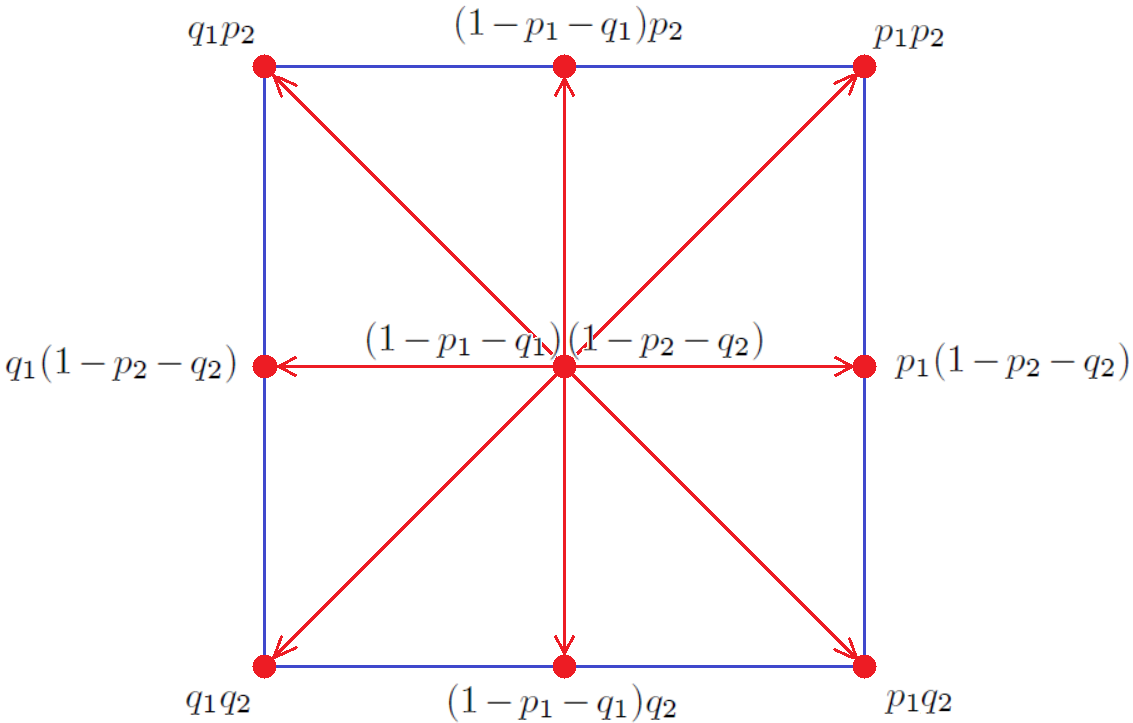
Refer to caption
Figure 6.2: Random walk in a bidimensional lattice.

Let 𝒏=(n1,…,nd)∈ℕd{\boldsymbol{n}}=(n_{1},\ldots,n_{d})\in\mathbb{N}^{d} and N⁡(𝒏)=∏i=1dniN({\boldsymbol{n}})=\prod_{i=1}^{d}n_{i}. We denote by {𝟏,…,𝒏}\{\mathbf{1},\ldots,{\boldsymbol{n}}\} the multi-index range {𝒊∈ℕd: 1≤𝒊≤𝒏}\{{\boldsymbol{i}}\in\mathbb{N}^{d}:\>\mathbf{1}\leq{\boldsymbol{i}}\leq{\boldsymbol{n}}\}, where 𝟏=(1,…,1)\mathbf{1}=(1,\ldots,1) and inequalities between vectors such as 𝒊≤𝒏{\boldsymbol{i}}\leq{\boldsymbol{n}} must be interpreted componentwise. When writing 𝒊=𝟏,…,𝒏{\boldsymbol{i}}=\mathbf{1},\ldots,{\boldsymbol{n}}, we mean that 𝒊{\boldsymbol{i}} varies from 𝟏\mathbf{1} to 𝒏{\boldsymbol{n}} over the multi-index range {𝟏,…,𝒏}\{\mathbf{1},\ldots,{\boldsymbol{n}}\} following the standard lexicographic ordering:

[…​[[(i1,…,id)]id=1,…,nd]id−1=1,…,nd−1​…]i1=1,…,n1.\Bigl[\ \ldots\ \bigl[\ [\>(i_{1},\ldots,i_{d})\>]_{i_{d}=1,\ldots,n_{d}}\ \bigr]_{i_{d-1}=1,\ldots,n_{d-1}}\ \ldots\ \Bigr]_{i_{1}=1,\ldots,n_{1}}.

We refer the reader to [20, Section 2.1.2] for more details on the multi-index notation.

Consider a discrete-time Markov chain with N⁡(𝒏)N({\boldsymbol{n}}) states 𝟏,…,𝒏\mathbf{1},\ldots,{\boldsymbol{n}} and with matrix of transition probabilities

P𝒏,𝒑,𝒒=⨂r=1dPnr,pr,qr,P_{{\boldsymbol{n}},{\boldsymbol{p}},{\boldsymbol{q}}}=\bigotimes_{r=1}^{d}P_{n_{r},p_{r},q_{r}},

where

  • •

    𝒑=(p1,…,pd){\boldsymbol{p}}=(p_{1},\ldots,p_{d}) and 𝒒=(q1,…,qd){\boldsymbol{q}}=(q_{1},\ldots,q_{d}) satisfy 𝒑,𝒒>𝟎{\boldsymbol{p}},{\boldsymbol{q}}>\mathbf{0} and 𝒑+𝒒≤𝟏{\boldsymbol{p}}+{\boldsymbol{q}}\leq\mathbf{1},

  • •

    the matrix Pnr,pr,qrP_{n_{r},p_{r},q_{r}} is defined by (6.4) for (n,p,q)=(nr,pr,qr)(n,p,q)=(n_{r},p_{r},q_{r}),

  • •

    ⨂\bigotimes denotes the tensor (Kronecker) product.

Markov chains of this kind are often referred to as random walks in the dd-dimensional lattice {𝟏,…,𝒏}\{\mathbf{1},\ldots,{\boldsymbol{n}}\}. They are a generalization of the unidimensional random walks discussed in Section 6.2. By the properties of tensor products [20, Section 2.5], for all 𝒊,𝒋=𝟏,…,𝒏{\boldsymbol{i}},{\boldsymbol{j}}=\mathbf{1},\ldots,{\boldsymbol{n}}, the probability of going from state 𝒊{\boldsymbol{i}} to state 𝒋{\boldsymbol{j}} is given by

(P𝒏,𝒑,𝒒)𝒊​𝒋=∏r=1d(Pnr,pr,qr)ir​jr,(P_{{\boldsymbol{n}},{\boldsymbol{p}},{\boldsymbol{q}}})_{{\boldsymbol{i}}{\boldsymbol{j}}}=\prod_{r=1}^{d}(P_{n_{r},p_{r},q_{r}})_{i_{r}j_{r}},

and it is equal to the product for r=1,…,dr=1,\ldots,d of the probability of going from state iri_{r} to state jrj_{r} in a unidimensional random walk with transition matrix Pnr,pr,qrP_{n_{r},p_{r},q_{r}} as considered in Section 6.2. In short, a dd-dimensional random walk is the result of dd independent unidimensional random walks (one for each space dimension); see Figure 6.2 for a bidimensional illustration.

By the properties of tensor products and the results of Section 6.2, we can immediately obtain the eigendecomposition of P𝒏,𝒑,𝒒⊤P_{{\boldsymbol{n}},{\boldsymbol{p}},{\boldsymbol{q}}}^{\top}. In particular, the eigenpairs of P𝒏,𝒑,𝒒⊤P_{{\boldsymbol{n}},{\boldsymbol{p}},{\boldsymbol{q}}}^{\top} are given by (μ𝒌,𝐰𝒌)(\mu_{\boldsymbol{k}},{\mathbf{w}}_{\boldsymbol{k}}), 𝒌=𝟎,…,𝒏−𝟏{\boldsymbol{k}}=\mathbf{0},\ldots,{\boldsymbol{n}}-\mathbf{1}, where

μ𝒌=∏r=1dμkr,𝐰𝒌=⨂r=1d𝐰kr,\mu_{\boldsymbol{k}}=\prod_{r=1}^{d}\mu_{k_{r}},\qquad{\mathbf{w}}_{\boldsymbol{k}}=\bigotimes_{r=1}^{d}{\mathbf{w}}_{k_{r}},

and (μkr,𝐰kr)(\mu_{k_{r}},{\mathbf{w}}_{k_{r}}) is defined by (6.5)–(6.6) for (k,n,p,q,α)=(kr,nr,pr,qr,αr)(k,n,p,q,\alpha)=(k_{r},n_{r},p_{r},q_{r},\alpha_{r}) with αr=pr/qr\alpha_{r}=\sqrt{p_{r}/q_{r}}.

Remark 6.5 (Steady-State Distribution).

The steady-state distribution of the dd-dimensional random walk is given by

𝐰𝟎‖𝐰𝟎‖1=⨂r=1d1−βr1−βrnr​[1,βr,βr2,…,βrnr−1]⊤,βr=αr2,\frac{{\mathbf{w}}_{\mathbf{0}}}{\|{\mathbf{w}}_{\mathbf{0}}\|_{1}}=\bigotimes_{r=1}^{d}\frac{1-\beta_{r}}{1-\beta_{r}^{n_{r}}}\bigl[1,\beta_{r},\beta_{r}^{2},\ldots,\beta_{r}^{n_{r}-1}\bigr]^{\top},\qquad\beta_{r}=\alpha_{r}^{2},

i.e., it is the tensor product of the steady-state distributions of the individual unidimensional random walks that compose it.

6.4 Multidimensional Diffusion Processes

Consider a dd-dimensional diffusion process, where the diffusions in each dimension are independent of each other and subject to a reflecting boundary condition at each side. We assume for simplicity that, for every r=1,…,dr=1,\ldots,d, the direction xrx_{r} is discretized uniformly with nrn_{r} nodes separated by a discretization step Δr>0\Delta_{r}>0. This discretization gives rise to a n1×⋯×ndn_{1}\times\cdots\times n_{d} lattice whose points 𝐱𝒊{\mathbf{x}}_{\boldsymbol{i}} are naturally indexed by a multi-index 𝒊=𝟏,…,𝒏{\boldsymbol{i}}=\mathbf{1},\ldots,{\boldsymbol{n}}, with 𝒏=(n1,…,nd){\boldsymbol{n}}=(n_{1},\ldots,n_{d}). The diffusion in direction xrx_{r} is a Brownian motion characterized by two parameters: a drift μr∈ℝ\mu_{r}\in\mathbb{R} and a variance σr2>0\sigma_{r}^{2}>0. For the direction xrx_{r}, the infinitesimal generator Lnr,μr,σrL_{n_{r},\mu_{r},\sigma_{r}} coincides with the generator of a 1-dimensional diffusion process with drift μr\mu_{r} and variance σr2\sigma_{r}^{2} discretized uniformly with nrn_{r} nodes separated by a discretization step Δr\Delta_{r}. In formulas, Lnr,μr,σrL_{n_{r},\mu_{r},\sigma_{r}} is an nr×nrn_{r}\times n_{r} matrix, which in the case μr≤0\mu_{r}\leq 0 is given by

Lnr,μr,σr\displaystyle L_{n_{r},\mu_{r},\sigma_{r}} =μrΔr​[0−11−11⋱⋱−11]+σr22​Δr2​[−111−21⋱⋱⋱1−211−1]=Qnr,λ~r,μ~r,\displaystyle=\frac{\mu_{r}}{\Delta_{r}}\left[\begin{array}[]{rrrrr}0&&&&\\ -1&1&&&\\ &-1&1&&\\ &&\ddots&\ddots&\\ &&&-1&1\end{array}\right]+\frac{\sigma_{r}^{2}}{2\Delta_{r}^{2}}\left[\begin{array}[]{rrrrr}-1&1&&&\\ 1&-2&1&&\\ &\ddots&\ddots&\ddots&\\ &&1&-2&1\\ &&&1&-1\\ \end{array}\right]=Q_{n_{r},\tilde{\lambda}_{r},\tilde{\mu}_{r}},

where λ~r=σr22​Δr2\displaystyle\tilde{\lambda}_{r}=\frac{\sigma_{r}^{2}}{2\Delta_{r}^{2}}, μ~r=σr22​Δr2−μrΔr\displaystyle\tilde{\mu}_{r}=\frac{\sigma_{r}^{2}}{2\Delta_{r}^{2}}-\frac{\mu_{r}}{\Delta_{r}}, and Qn,λ,μQ_{n,\lambda,\mu} is defined in (6.1); and in the case μr≥0\mu_{r}\geq 0 is given by

Lnr,μr,σr\displaystyle L_{n_{r},\mu_{r},\sigma_{r}} =μrΔr​[−11−11⋱⋱−110]+σr22​Δr2​[−111−21⋱⋱⋱1−211−1]=Qnr,λ~r,μ~r,\displaystyle=\frac{\mu_{r}}{\Delta_{r}}\left[\begin{array}[]{rrrrr}-1&1&&&\\ &-1&1&&\\ &&\ddots&\ddots&\\ &&&-1&1\\ &&&&0\end{array}\right]+\frac{\sigma_{r}^{2}}{2\Delta_{r}^{2}}\left[\begin{array}[]{rrrrr}-1&1&&&\\ 1&-2&1&&\\ &\ddots&\ddots&\ddots&\\ &&1&-2&1\\ &&&1&-1\\ \end{array}\right]=Q_{n_{r},\tilde{\lambda}_{r},\tilde{\mu}_{r}},

where λ~r=σr22​Δr2+μrΔr\displaystyle\tilde{\lambda}_{r}=\frac{\sigma_{r}^{2}}{2\Delta_{r}^{2}}+\frac{\mu_{r}}{\Delta_{r}}, μ~r=σr22​Δr2\displaystyle\tilde{\mu}_{r}=\frac{\sigma_{r}^{2}}{2\Delta_{r}^{2}}, and Qn,λ,μQ_{n,\lambda,\mu} is defined in (6.1). In short,

Lnr,μr,σr=Qnr,λ~r,μ~r,λ~r={σr22​Δr2,if μr≤0,σr22​Δr2+μrΔr,if μr≥0,μ~r={σr22​Δr2−μrΔr,if μr≤0,σr22​Δr2,if μr≥0.L_{n_{r},\mu_{r},\sigma_{r}}=Q_{n_{r},\tilde{\lambda}_{r},\tilde{\mu}_{r}},\qquad\tilde{\lambda}_{r}=\left\{\begin{aligned} &\frac{\sigma_{r}^{2}}{2\Delta_{r}^{2}},&&&\mbox{if $\mu_{r}\leq 0$},\\ &\frac{\sigma_{r}^{2}}{2\Delta_{r}^{2}}+\frac{\mu_{r}}{\Delta_{r}},&&&\mbox{if $\mu_{r}\geq 0$},\end{aligned}\right.\qquad\tilde{\mu}_{r}=\left\{\begin{aligned} &\frac{\sigma_{r}^{2}}{2\Delta_{r}^{2}}-\frac{\mu_{r}}{\Delta_{r}},&&&\mbox{if $\mu_{r}\leq 0$},\\ &\frac{\sigma_{r}^{2}}{2\Delta_{r}^{2}},&&&\mbox{if $\mu_{r}\geq 0$}.\end{aligned}\right.

The differential operator (infinitesimal generator) of the dd-dimensional diffusion process is given by

L𝒏,𝝁,𝝈\displaystyle L_{{\boldsymbol{n}},{\boldsymbol{\mu}},{\boldsymbol{\sigma}}} =∑i=1dIn1⊗⋯⊗Ini−1⊗Lnr,μr,σr⊗Ini+1⊗⋯⊗Ind,\displaystyle=\sum_{i=1}^{d}I_{n_{1}}\otimes\cdots\otimes I_{n_{i-1}}\otimes L_{n_{r},\mu_{r},\sigma_{r}}\otimes I_{n_{i+1}}\otimes\cdots\otimes I_{n_{d}}, (6.7)

where 𝝁=(μ1,…,μd){\boldsymbol{\mu}}=(\mu_{1},\ldots,\mu_{d}) and 𝝈=(σ1,…,σd){\boldsymbol{\sigma}}=(\sigma_{1},\ldots,\sigma_{d}). More details on the discretized multidimensional diffusion process considered here will be given in Section 6.5 along with an economics application; for more on diffusion processes, see [5] for a mathematical treatment and [2, 3, 17] for an economical application-oriented approach.

By the properties of tensor products and the results of Section 6.1, we can immediately obtain the eigendecomposition of L𝒏,𝝁,𝝈⊤L_{{\boldsymbol{n}},{\boldsymbol{\mu}},{\boldsymbol{\sigma}}}^{\top}. In particular, the eigenpairs of L𝒏,𝝁,𝝈⊤L_{{\boldsymbol{n}},{\boldsymbol{\mu}},{\boldsymbol{\sigma}}}^{\top} are given by (ν𝒌,𝐰𝒌)(\nu_{\boldsymbol{k}},{\mathbf{w}}_{\boldsymbol{k}}), 𝒌=𝟎,…,𝒏−𝟏{\boldsymbol{k}}=\mathbf{0},\ldots,{\boldsymbol{n}}-\mathbf{1}, where

ν𝒌=∑r=1dνkr,𝐰𝒌=⨂r=1d𝐰kr,\nu_{\boldsymbol{k}}=\sum_{r=1}^{d}\nu_{k_{r}},\qquad{\mathbf{w}}_{\boldsymbol{k}}=\bigotimes_{r=1}^{d}{\mathbf{w}}_{k_{r}}, (6.8)

and (νkr,𝐰kr)(\nu_{k_{r}},{\mathbf{w}}_{k_{r}}) is defined by (6.2)–(6.3) for (k,n,λ,μ,τ)=(kr,nr,λ~r,μ~r,τ~r)(k,n,\lambda,\mu,\tau)=(k_{r},n_{r},\tilde{\lambda}_{r},\tilde{\mu}_{r},\tilde{\tau}_{r}) with τ~r=λ~r/μ~r\tilde{\tau}_{r}=\sqrt{\tilde{\lambda}_{r}/\tilde{\mu}_{r}}.

Remark 6.6 (Steady-State Distribution).

The steady-state distribution of the dd-dimensional diffusion process generated by L𝒏,𝝁,𝝈L_{{\boldsymbol{n}},{\boldsymbol{\mu}},{\boldsymbol{\sigma}}}, i.e., the normalized positive eigenvector of L𝒏,𝝁,𝝈⊤L_{{\boldsymbol{n}},{\boldsymbol{\mu}},{\boldsymbol{\sigma}}}^{\top} associated with the eigenvalue 00, is given by

𝐩=𝐰𝟎‖𝐰𝟎‖1=⨂r=1d1−ρ~r1−ρ~rnr​[1,ρ~r,ρ~r2,…,ρ~rnr−1]⊤=⨂r=1d𝐩r,ρ~r=τ~r2,{\mathbf{p}}=\frac{{\mathbf{w}}_{\mathbf{0}}}{\|{\mathbf{w}}_{\mathbf{0}}\|_{1}}=\bigotimes_{r=1}^{d}\frac{1-\tilde{\rho}_{r}}{1-\tilde{\rho}_{r}^{n_{r}}}\bigl[1,\tilde{\rho}_{r},\tilde{\rho}_{r}^{2},\ldots,\tilde{\rho}_{r}^{n_{r}-1}\bigr]^{\top}=\bigotimes_{r=1}^{d}{\mathbf{p}}_{r},\qquad\tilde{\rho}_{r}=\tilde{\tau}_{r}^{2}, (6.9)

i.e., it is the tensor product of the steady-state distributions 𝐩r{\mathbf{p}}_{r} of the individual unidimensional diffusion processes generated by the operators Lnr,μr,σrL_{n_{r},\mu_{r},\sigma_{r}}, r=1,…,dr=1,\ldots,d.

6.5 Dynamics of Wealth and Income Inequality

In this section, we present an economic application of the results obtained in Section 6.4. We begin with an overview of the topic, which may not be so familiar to non-economists.

6.5.1 Modeling the Evolution of Wealth and Income

The sources of the vast wealth and income inequality is a key topic of study within macroeconomics and finance; see [2, 3, 4, 6, 7] for empirical evidence and modeling approaches. Central to the questions of inequality are:

  • •

    what is the source of heterogeneity that drives the stationary distribution of income or wealth?

  • •

    how would the income or wealth distribution evolve over time given aggregate changes?

For example, researchers can ask how the stationary distribution of wealth will change—and how long it will take to be reached—given experiments such as a new income tax, technological changes driving more volatile wages, or increases in the returns on an asset such as housing. Methodologically, the analysis of income inequality is done through examining the stationary distribution of discrete- or continuous-time stochastic processes associated with income or wealth. Typically, researchers act as follows.

  • •

    They choose a stochastic process for the assets of interest (for example, housing wealth, human wealth (i.e., wages), stocks, bonds, social security income, etc.).

  • •

    They use data to estimate the parameters of the stochastic process for that “portfolio” of assets; see [2] for a survey intended to bridge the continuous-time versions of these models. In some cases, the parameters are derived from optimal control of a Hamilton–Jacobi–Bellman equation [2, 3, 7].

  • •

    They solve for the stationary distribution associated with the stochastic process. In this way, they can examine properties of the distribution, relate it back to the data, and conduct hypotheticals on the impact of policy.

With this approach, the emphasis on the steady-state distribution has come out of necessity. Even the speed of convergence towards the steady state has recently become an active research field; see [18] for a theory of the convergence rates largely focused on infinite-dimensional univariate models, and [25] for earlier evidence and theory on transition rates of the firm size distribution (methodologically, much of the literature on income/wealth inequality is similar to the firm dynamics literature, where the goal is to understand the distribution of firm sizes or productivity as well as the role of firm or worker heterogeneity in generating that distribution [17, 25, 26]).

6.5.2 Continuous-State Formulation

Consider a portfolio of dd assets 𝐗⁡(t)=(X1​(t),…,Xd​(t)){\mathbf{X}}(t)=(X_{1}(t),\ldots,X_{d}(t)) (e.g., housing wealth, wage income, social security, etc.). We emphasize the dependence on tt because the assets evolve over time. We assume that X1​(t),…,Xd​(t)X_{1}(t),\ldots,X_{d}(t) are dd independent Brownian motions with drifts μ1,…,μd\mu_{1},\ldots,\mu_{d} and variances σ12,…,σd2\sigma_{1}^{2},\ldots,\sigma_{d}^{2}. Without loss of generality, we also assume that X1​(t),…,Xd​(t)X_{1}(t),\ldots,X_{d}(t) take values in [0,1][0,1], so that the portfolio 𝐗⁡(t){\mathbf{X}}(t) determining an individual’s wealth is an element 𝐱=(x1,…,xd)∈[0,1]d{\mathbf{x}}=(x_{1},\ldots,x_{d})\in[0,1]^{d} at any time tt. The resulting stochastic process for the considered set of assets is a dd-dimensional Brownian motion with drifts 𝝁=(μ1,…,μd){\boldsymbol{\mu}}=(\mu_{1},\ldots,\mu_{d}) and variances 𝝈2=(σ12,…,σd2){\boldsymbol{\sigma}}^{2}=(\sigma_{1}^{2},\ldots,\sigma_{d}^{2}), and with the edges of the hypercube [0,1]d[0,1]^{d} acting as reflecting barriers. The probability density function pr​(xr,t)p_{r}(x_{r},t) for the asset Xr​(t)X_{r}(t) at time tt is determined by the Kolmogorov forward equation (Fokker–Planck equation)

∂pr∂t​(xr,t)\displaystyle\frac{\partial p_{r}}{\partial t}(x_{r},t) =−μr​∂pr∂xr​(xr,t)+σr22​∂2pr∂xr2​(xr,t)\displaystyle=-\mu_{r}\frac{\partial p_{r}}{\partial x_{r}}(x_{r},t)+\frac{\sigma_{r}^{2}}{2}\,\frac{\partial^{2}p_{r}}{\partial x_{r}^{2}}(x_{r},t) (6.10)

subject to the boundary conditions induced by reflecting boundaries at 00 and 11:

0\displaystyle 0 =−μrpr(xr,t)+σr22∂pr∂xr(xr,t),xr=0,1.\displaystyle=-\mu_{r}p_{r}(x_{r},t)+\frac{\sigma_{r}^{2}}{2}\,\frac{\partial p_{r}}{\partial x_{r}}(x_{r},t),\qquad x_{r}=0,1. (6.11)

The objects of interest are the following.

  • •

    The stationary density function pr​(xr)p_{r}(x_{r}), that is, the density function independent of tt satisfying (6.10)–(6.11). The function pr​(xr)p_{r}(x_{r}) does not evolve over time and determines the limiting (equilibrium) density function p(𝐱)=p1(x1)⋯pd(xd)p({\mathbf{x}})=p_{1}(x_{1})\cdots p_{d}(x_{d}) characterizing the steady-state probability distribution of the process.

  • •

    Any function WW that maps a state 𝐱∈[0,1]d{\mathbf{x}}\in[0,1]^{d} to a scalar “wealth” or “payoff” W⁡(𝐱)W({\mathbf{x}}). 11 1  As an example in the case d=2d=2, asset X1​(t)X_{1}(t) could be housing wealth at time tt and asset X2​(t)X_{2}(t) could be bank holdings at time tt in an individual’s portfolio. If w1w_{1} is the per-unit value of a house and w2w_{2} the per-unit value of a bank holding, then the “wealth” of an individual in state (X1,X2)=(x1,x2)(X_{1},X_{2})=(x_{1},x_{2}) is W⁡(x1,x2)=w1​x1+w2​x2W(x_{1},x_{2})=w_{1}x_{1}+w_{2}x_{2}. Clearly, W⁡(𝐗⁡(t))W({\mathbf{X}}(t)) is a random variable evolving over time together with the portfolio 𝐗⁡(t){\mathbf{X}}(t), and we are interested in quantities like the average wealth 𝔼⁡[W⁡(𝐗)]\mathbb{E}[W({\mathbf{X}})] and the wealth variance Var⁡[W⁡(𝐗)]{\rm Var}[W({\mathbf{X}})] computed in the steady-state distribution p⁡(𝐱)p({\mathbf{x}}), that is,

    𝔼⁡[W⁡(𝐗)]\displaystyle\mathbb{E}[W({\mathbf{X}})] =∫[0,1]2W⁡(𝐱)​p​(𝐱)​𝑑𝐱,\displaystyle=\int_{[0,1]^{2}}W({\mathbf{x}})p({\mathbf{x}}){\rm d}{\mathbf{x}},
    Var⁡[W⁡(𝐗)]\displaystyle{\rm Var}[W({\mathbf{X}})] =𝔼⁡[W​(𝐗)2]−𝔼​[W⁡(𝐗)]2=∫[0,1]2W​(𝐱)2​p​(𝐱)​𝑑𝐱−(∫[0,1]2W⁡(𝐱)​p​(𝐱)​𝑑𝐱)2.\displaystyle=\mathbb{E}[W({\mathbf{X}})^{2}]-\mathbb{E}[W({\mathbf{X}})]^{2}=\int_{[0,1]^{2}}W({\mathbf{x}})^{2}p({\mathbf{x}}){\rm d}{\mathbf{x}}-\biggl(\int_{[0,1]^{2}}W({\mathbf{x}})p({\mathbf{x}}){\rm d}{\mathbf{x}}\biggr)^{2}.

6.5.3 Discrete-State Formulation

Suppose we discretize the hypercube [0,1]d[0,1]^{d} by introducing a n1×⋯×ndn_{1}\times\cdots\times n_{d} lattice with nrn_{r} points in direction xrx_{r} separated by a discretization step Δr>0\Delta_{r}>0, as in Section 6.4. This essentially means that we allow each random variable (asset) Xr​(t)X_{r}(t) to assume only a finite number of values. Consequently, the portfolio 𝐗⁡(t)=(X1​(t),…,Xr​(t)){\mathbf{X}}(t)=(X_{1}(t),\ldots,X_{r}(t)) can only be in a finite number of states 𝐱𝟏,…,𝐱𝒏{\mathbf{x}}_{\mathbf{1}},\ldots,{\mathbf{x}}_{\boldsymbol{n}}. The use of upwind finite differences allow us to convert the 2​d2d PDEs (6.10)–(6.11) to a unique system of ODEs

d​𝐩d​t​(t)\displaystyle\frac{{\rm d}{\mathbf{p}}}{{\rm d}t}(t) =L𝒏,𝝁,𝝈⊤​𝐩​(t)\displaystyle=L_{{\boldsymbol{n}},{\boldsymbol{\mu}},{\boldsymbol{\sigma}}}^{\top}\mathbf{p}(t) (6.12)

subject to an initial condition 𝐩⁡(0){\mathbf{p}}(0), where L𝒏,𝝁,𝝈L_{{\boldsymbol{n}},{\boldsymbol{\mu}},{\boldsymbol{\sigma}}} is the infinitesimal generator (6.7) and 𝐩𝒊​(t){\mathbf{p}}_{\boldsymbol{i}}(t) is the probability that the portfolio 𝐗⁡(t){\mathbf{X}}(t) is in state 𝐱𝒊{\mathbf{x}}_{\boldsymbol{i}} at time tt. After this discretization, the continuous-state continuous-time Markov process of Section 6.5.2 is changed into a discrete-state continuous-time Markov chain. Here, the objects of interest are the discrete counterparts of those mentioned in Section 6.5.2, i.e., the following.

  • •

    The stationary distribution 𝐩=(p𝟏,…,p𝒏){\mathbf{p}}=(p_{\mathbf{1}},\ldots,p_{\boldsymbol{n}}) of the process, that is, the probability vector independent of tt satisfying (6.12). Clearly, 𝐩{\mathbf{p}} is the normalized positive eigenvector of L𝒏,𝝁,𝝈⊤L_{{\boldsymbol{n}},{\boldsymbol{\mu}},{\boldsymbol{\sigma}}}^{\top} associated with the zero eigenvalue and is given by (6.9).

  • •

    Any function WW that maps a state 𝐱𝒊∈[0,1]d{\mathbf{x}}_{\boldsymbol{i}}\in[0,1]^{d} to a scalar “wealth” or “payoff” W⁡(𝐱𝒊)=W𝒊W({\mathbf{x}}_{\boldsymbol{i}})=W_{\boldsymbol{i}}. Clearly, W⁡(𝐗⁡(t))W({\mathbf{X}}(t)) is a random variable evolving over time together with the portfolio 𝐗⁡(t){\mathbf{X}}(t), and we are interested in quantities like the average wealth 𝔼⁡[W⁡(𝐗)]\mathbb{E}[W({\mathbf{X}})] and the wealth variance Var⁡[W⁡(𝐗)]{\rm Var}[W({\mathbf{X}})] computed in the steady-state distribution 𝐩{\mathbf{p}}, that is,

    𝔼⁡[W⁡(𝐗)]\displaystyle\mathbb{E}[W({\mathbf{X}})] =𝐖⋅𝐩,\displaystyle={\mathbf{W}}\cdot{\mathbf{p}}, (6.13)
    Var⁡[W⁡(𝐗)]\displaystyle{\rm Var}[W({\mathbf{X}})] =𝔼⁡[W​(𝐗)2]−𝔼​[W⁡(𝐗)]2=𝐖2⋅𝐩−(𝐖⋅𝐩)2,\displaystyle=\mathbb{E}[W({\mathbf{X}})^{2}]-\mathbb{E}[W({\mathbf{X}})]^{2}={\mathbf{W}}^{2}\cdot{\mathbf{p}}-({\mathbf{W}}\cdot{\mathbf{p}})^{2}, (6.14)

    where 𝐖=(W𝟏,…,W𝒏){\mathbf{W}}=(W_{\mathbf{1}},\ldots,W_{\boldsymbol{n}}) is the vector (tensor) of payoffs and 𝐖2{\mathbf{W}}^{2} is the componentwise square of 𝐖{\mathbf{W}} (in general, operations on vectors that have no meaning in themselves must be interpreted in the componentwise sense).

Considering that 𝐩{\mathbf{p}} is known from (6.9), formulas (6.13)–(6.14) allow us to compute both the average wealth and the wealth variance in the steady state of the process. This lets us analyze different hypothetical scenarios. For example, if the drift μ1\mu_{1} of the housing component of an individual’s portfolio increases, what would the impact be on the average wealth? Alternatively, we could ask how the wealth variance (a simple measure of inequality) would change if the variance of wages increases.

6.5.4 Convergence Speed to the Steady State

The results of Section 6.4 allow us to quantify the convergence speed to the steady state of the Markov chain presented in Section 6.5.3. Indeed, as we know from Section 6.4, all nonzero eigenvalues of L𝒏,𝝁,𝝈L_{{\boldsymbol{n}},{\boldsymbol{\mu}},{\boldsymbol{\sigma}}} are negative and the largest of them, i.e., the second largest eigenvalue after 0, is given by

ν=maxr=1,…,d⁡(−λ~r−μ~r+2​λ~r​μ~r​cos⁡πnr).\nu=\max_{r=1,\ldots,d}\Bigl(-\tilde{\lambda}_{r}-\tilde{\mu}_{r}+2\sqrt{\tilde{\lambda}_{r}\tilde{\mu}_{r}}\cos\frac{\pi}{n_{r}}\Bigr). (6.15)

The second eigenvalue provides a measure of the convergence speed towards the steady state. The reason is the following: for essentially every choice of the initial distribution 𝐩⁡(0){\mathbf{p}}(0), the quantities 𝐩⁡(t){\mathbf{p}}(t), 𝔼⁡[W⁡(𝐗⁡(t))]\mathbb{E}[W({\mathbf{X}}(t))], Var⁡[W⁡(𝐗⁡(t))]{\rm Var}[W({\mathbf{X}}(t))] converge to their stationary counterparts 𝐩{\mathbf{p}}, 𝔼⁡[W⁡(𝐗)]\mathbb{E}[W({\mathbf{X}})], Var⁡[W⁡(𝐗)]{\rm Var}[W({\mathbf{X}})] in (6.9), (6.13), (6.14) with asymptotic convergence rates given by

limt→∞dd​t​ln⁡‖𝐩⁡(t)−𝐩‖2\displaystyle\lim_{t\to\infty}\frac{{\rm d}}{{\rm d}t}\ln\|{\mathbf{p}}(t)-{\mathbf{p}}\|_{2} =ν,\displaystyle=\nu, (6.16)
limt→∞dd​t​ln​|𝔼⁡[W⁡(𝐗⁡(t))]−𝔼⁡[W⁡(𝐗)]|\displaystyle\lim_{t\to\infty}\frac{{\rm d}}{{\rm d}t}\ln|\mathbb{E}[W({\mathbf{X}}(t))]-\mathbb{E}[W({\mathbf{X}})]| =ν,\displaystyle=\nu, (6.17)
limt→∞dd​t​ln​|Var⁡[W⁡(𝐗⁡(t))]−Var⁡[W⁡(𝐗)]|\displaystyle\lim_{t\to\infty}\frac{{\rm d}}{{\rm d}t}\ln|{\rm Var}[W({\mathbf{X}}(t))]-{\rm Var}[W({\mathbf{X}})]| =ν.\displaystyle=\nu. (6.18)

For more details on the role of the second eigenvalue as a measure of the asymptotic convergence rate towards the steady state, see, e.g., [17] and [24, Section 7.2].

6.5.5 Derivatives with Respect to Drifts and Variances

For the convenience of economists, we here report the derivatives of the steady-state distribution 𝐩{\mathbf{p}} in (6.9), the average wealth 𝔼⁡[W⁡(𝐗)]\mathbb{E}[W({\mathbf{X}})] in (6.13), and the wealth variance Var⁡[W⁡(𝐗)]{\rm Var}[W({\mathbf{X}})] in (6.14) with respect to the drifts 𝝁{\boldsymbol{\mu}} and the variances 𝝈2{\boldsymbol{\sigma}}^{2}. For r=1,…,dr=1,\ldots,d, we have

∂ρ~r∂μr\displaystyle\frac{\partial\tilde{\rho}_{r}}{\partial\mu_{r}} ={σr22​Δr3​μ~r2=2​Δr​σr2(σr2−2​Δr​μr)2,if μr≤0,1Δr​μ~r=2​Δrσr2,if μr≥0,\displaystyle=\left\{\begin{aligned} &\frac{\sigma_{r}^{2}}{2\Delta_{r}^{3}\tilde{\mu}_{r}^{2}}=\frac{2\Delta_{r}\sigma_{r}^{2}}{(\sigma_{r}^{2}-2\Delta_{r}\mu_{r})^{2}},&&&\mbox{if $\mu_{r}\leq 0$},\\ &\frac{1}{\Delta_{r}\tilde{\mu}_{r}}=\frac{2\Delta_{r}}{\sigma_{r}^{2}},&&&\mbox{if $\mu_{r}\geq 0$},\end{aligned}\right.
∂ρ~r∂σr2\displaystyle\frac{\partial\tilde{\rho}_{r}}{\partial\sigma_{r}^{2}} =−μr2​Δr3​μ~r2,\displaystyle=-\frac{\mu_{r}}{2\Delta_{r}^{3}\tilde{\mu}_{r}^{2}},
∂𝐩r∂ρ~r\displaystyle\frac{\partial{\mathbf{p}}_{r}}{\partial\tilde{\rho}_{r}} =(1−nr)​ρ~rnr+nr​ρ~rnr−1−1(1−ρ~rnr)2​[1,ρ~r,ρ~r2,…,ρ~rnr−1]⊤+1−ρ~r1−ρ~rnr​[0,1,2​ρ~r,…,(nr−1)​ρ~rnr−2]⊤,\displaystyle=\frac{(1-n_{r})\tilde{\rho}_{r}^{n_{r}}+n_{r}\tilde{\rho}_{r}^{n_{r}-1}-1}{(1-\tilde{\rho}_{r}^{n_{r}})^{2}}\bigl[1,\tilde{\rho}_{r},\tilde{\rho}_{r}^{2},\ldots,\tilde{\rho}_{r}^{n_{r}-1}\bigr]^{\top}+\frac{1-\tilde{\rho}_{r}}{1-\tilde{\rho}_{r}^{n_{r}}}\bigl[0,1,2\tilde{\rho}_{r},\ldots,(n_{r}-1)\tilde{\rho}_{r}^{n_{r}-2}\bigr]^{\top},
∂𝐩r∂μr\displaystyle\frac{\partial{\mathbf{p}}_{r}}{\partial\mu_{r}} =∂ρ~r∂μr​∂𝐩r∂ρ~r,\displaystyle=\frac{\partial\tilde{\rho}_{r}}{\partial\mu_{r}}\,\frac{\partial{\mathbf{p}}_{r}}{\partial\tilde{\rho}_{r}},
∂𝐩r∂σr2\displaystyle\frac{\partial{\mathbf{p}}_{r}}{\partial\sigma_{r}^{2}} =∂ρ~r∂σr2​∂𝐩r∂ρ~r,\displaystyle=\frac{\partial\tilde{\rho}_{r}}{\partial\sigma_{r}^{2}}\,\frac{\partial{\mathbf{p}}_{r}}{\partial\tilde{\rho}_{r}},
∂𝐩∂μr\displaystyle\frac{\partial{\mathbf{p}}}{\partial\mu_{r}} =𝐩1⊗⋯⊗𝐩r−1⊗∂𝐩r∂μr⊗𝐩r+1⊗⋯⊗𝐩d,\displaystyle={\mathbf{p}}_{1}\otimes\cdots\otimes{\mathbf{p}}_{r-1}\otimes\frac{\partial{\mathbf{p}}_{r}}{\partial\mu_{r}}\otimes{\mathbf{p}}_{r+1}\otimes\cdots\otimes{\mathbf{p}}_{d}, (6.19)
∂𝐩∂σr2\displaystyle\frac{\partial{\mathbf{p}}}{\partial\sigma_{r}^{2}} =𝐩1⊗⋯⊗𝐩r−1⊗∂𝐩r∂σr2⊗𝐩r+1⊗⋯⊗𝐩d,\displaystyle={\mathbf{p}}_{1}\otimes\cdots\otimes{\mathbf{p}}_{r-1}\otimes\frac{\partial{\mathbf{p}}_{r}}{\partial\sigma_{r}^{2}}\otimes{\mathbf{p}}_{r+1}\otimes\cdots\otimes{\mathbf{p}}_{d}, (6.20)
∂𝔼⁡[W⁡(𝐗)]∂μr\displaystyle\frac{\partial\mathbb{E}[W({\mathbf{X}})]}{\partial\mu_{r}} =𝐖⋅∂𝐩∂μr,\displaystyle={\mathbf{W}}\cdot\frac{\partial{\mathbf{p}}}{\partial\mu_{r}}, (6.21)
∂𝔼⁡[W⁡(𝐗)]∂σr2\displaystyle\frac{\partial\mathbb{E}[W({\mathbf{X}})]}{\partial\sigma_{r}^{2}} =𝐖⋅∂𝐩∂σr2,\displaystyle={\mathbf{W}}\cdot\frac{\partial{\mathbf{p}}}{\partial\sigma_{r}^{2}}, (6.22)
∂Var⁡[W⁡(𝐗)]∂μr\displaystyle\frac{\partial{\rm Var}[W({\mathbf{X}})]}{\partial\mu_{r}} =𝐖2⋅∂𝐩∂μr−2​(𝐖⋅𝐩)​(𝐖⋅∂𝐩∂μr),\displaystyle={\mathbf{W}}^{2}\cdot\frac{\partial{\mathbf{p}}}{\partial\mu_{r}}-2({\mathbf{W}}\cdot{\mathbf{p}})\Bigl({\mathbf{W}}\cdot\frac{\partial{\mathbf{p}}}{\partial\mu_{r}}\Bigr), (6.23)
∂Var⁡[W⁡(𝐗)]∂σr2\displaystyle\frac{\partial{\rm Var}[W({\mathbf{X}})]}{\partial\sigma_{r}^{2}} =𝐖2⋅∂𝐩∂σr2−2​(𝐖⋅𝐩)​(𝐖⋅∂𝐩∂σr2).\displaystyle={\mathbf{W}}^{2}\cdot\frac{\partial{\mathbf{p}}}{\partial\sigma_{r}^{2}}-2({\mathbf{W}}\cdot{\mathbf{p}})\Bigl({\mathbf{W}}\cdot\frac{\partial{\mathbf{p}}}{\partial\sigma_{r}^{2}}\Bigr). (6.24)
Refer to caption
Figure 6.3: Changes in moments of the wealth distribution. Parameters are chosen to be illustrative: μ1=μ2=0.01\mu_{1}=\mu_{2}=0.01, σ12=σ22=0.0025\sigma_{1}^{2}=\sigma_{2}^{2}=0.0025, and W⁡(x1,x2)=x1+x2W(x_{1},x_{2})=x_{1}+x_{2}.

We remark that the above derivatives are defined even in the case μr=0\mu_{r}=0 and their values in this case are obtained by taking the limit of the corresponding expression as μr→0\mu_{r}\to 0. The derivatives (6.19)–(6.20) enable an analysis of how the steady state changes when properties of the underlying process change. For example, if the volatility of housing prices σ12\sigma_{1}^{2} increases, equations (6.19)–(6.20) provide the resulting impact on the steady state. The derivatives (6.21)–(6.24) can be used to examine how key moments of the stationary distribution change. For example, a researcher could analyze the impact on the steady-state variance of the wealth distribution, i.e., Var⁡[W⁡(𝐗)]{\rm Var}[W({\mathbf{X}})], in the case where the volatility of housing prices σ12\sigma_{1}^{2} increases. Figure 6.3 illustrates this by showing how the mean and variance of the stationary wealth distribution change with respect to the parameters of the underlying stochastic process. The figure has been realized through a discretization of the square [0,1]2[0,1]^{2} by a n1×n2n_{1}\times n_{2} lattice with n1=n2=31n_{1}=n_{2}=31 points in each direction and (consequently) two equal discretization steps Δ1=Δ2=1/30\Delta_{1}=\Delta_{2}=1/30. It should be noted, however, that the graphs in Figure 6.3 do not really depend on n1n_{1} and n2n_{2}, because they converge to limiting graphs as n1,n2→∞n_{1},n_{2}\to\infty (and convergence is already reached for n1=n2=31n_{1}=n_{2}=31).

7 Conclusions and Perspectives

We have studied the spectral properties of the generator Tn,ε,φT_{n,\varepsilon,\varphi} of the τε,φ\tau_{\varepsilon,\varphi} algebra introduced by Bozzo and Di Fiore in the context of matrix displacement decomposition [13]. In particular:

  • •

    we have derived precise asymptotics for the outliers of Tn,ε,φT_{n,\varepsilon,\varphi} and the associated eigenvectors;

  • •

    we have obtained equations for the eigenvalues of Tn,ε,φT_{n,\varepsilon,\varphi}, which automatically provide also the eigenvectors of Tn,ε,φT_{n,\varepsilon,\varphi};

  • •

    we have computed the full eigendecomposition of Tn,ε,φT_{n,\varepsilon,\varphi} in the case ε​φ=1\varepsilon\varphi=1.

Finally, we have presented applications of our results to queuing models, random walks, diffusion processes, and economics, with a special emphasis on wealth/income inequality and portfolio dynamics. We conclude this paper by mentioning a few possible future lines of research.

  1. 1.

    The applications presented herein do not exhaust all possible applications of the τε,φ\tau_{\varepsilon,\varphi} algebra. For example, matrices belonging to this algebra for suitable choices of ε\varepsilon and φ\varphi arise in the discretization of differential equations by finite difference methods, finite element methods and, as recently discovered, isogeometric methods [16, Section 3]. A future research could take care of investigating further discretizations where τε,φ\tau_{\varepsilon,\varphi} matrices arise and, consequently, the results of this paper find applications.

  2. 2.

    On the economics side, Sections 6.4–6.5 are interesting and useful, but the reflected constant-coefficient diffusion process 𝐗⁡(t){\mathbf{X}}(t) that has been considered therein is not sufficient to understand top income inequality, since in that case researchers need alternative specifications [6, 18]. That said, there could be a large class of stochastic processes 𝐗^​(t)\hat{\mathbf{X}}(t) that can be mapped to 𝐗⁡(t){\mathbf{X}}(t) through an appropriate change of measure. Loosely, given a stochastic process 𝐗^​(t)\hat{\mathbf{X}}(t), let W^\hat{W} be a mapping such that W^​(𝐗^​(t))\hat{W}(\hat{\mathbf{X}}(t)) represents the “wealth” of an individual with portfolio 𝐗^​(t)\hat{\mathbf{X}}(t). Then, there may exist a change of measure ℙ→ℚ\mathbb{P}\to\mathbb{Q} (i.e., a Radon–Nikodym derivative d​ℚ/d​ℙ{\rm d}\mathbb{Q}/{\rm d}\mathbb{P}) mapping 𝐗^​(t)\hat{\mathbf{X}}(t) to 𝐗⁡(t){\mathbf{X}}(t) and W^​(𝐗^​(t))\hat{W}(\hat{\mathbf{X}}(t)) to W⁡(𝐗⁡(t))W({\mathbf{X}}(t)) for a suitable WW. If so, then the computation of, say, the average wealth 𝔼ℙ​[W^​(𝐗^)]\mathbb{E}_{\mathbb{P}}[\hat{W}(\hat{\mathbf{X}})] in the steady-state distribution of process 𝐗^​(t)\hat{\mathbf{X}}(t) could be traced back to computing the corresponding expectation 𝔼ℚ​[W​(𝐗)]\mathbb{E}_{\mathbb{Q}}[W({\mathbf{X}})] for process 𝐗⁡(t){\mathbf{X}}(t) as we have done in Section 6.5; see [14, Section 9.5] for an analysis of changes in probability measures and associated expectations, as well as for practical tools for working with such concepts. A careful investigation of all this topic may form the content of a future research that would extend the applicability of the results presented in this paper.

Acknowledgements

The authors wish to thank Carmine Di Fiore for useful discussions. This work has been supported by the MIUR Excellence Department Project awarded to the Department of Mathematics of the University of Rome Tor Vergata (CUP E83C18000100006), by the Beyond Borders Programme of the University of Rome Tor Vergata through the Project ASTRID (CUP E84I19002250005), by the Research Group GNCS (Gruppo Nazionale per il Calcolo Scientifico) of INdAM (Istituto Nazionale di Alta Matematica), and by the Swedish Research Council through the International Postdoc Grant (Registration Number 2019-00495).

References

  • [1]
  • [2] Achdou Y., Buera F. J., Lasry J.-M., Lions P.-L., Moll B. Partial differential equation models in macroeconomics. Philos. Trans. Royal Soc. A 372 (2014) 20130397.
  • [3] Achdou Y., Han J., Lasry J.-M., Lions P.-L., Moll B. Income and wealth distribution in macroeconomics: a continuous-time approach. Working Paper 23732, National Bureau of Economic Research (2017).
  • [4] Atkinson A. B., Piketty T., Saez E. Top incomes in the long run of history. J. Econ. Lit. 49 (2011) 3–71.
  • [5] Baldi P. Stochastic Calculus: An Introduction Through Theory and Exercises. Springer, Cham (2017).
  • [6] Benhabib J., Bisin A. Skewed wealth distributions: theory and empirics. J. Econ. Lit. 56 (2018) 1261–1291.
  • [7] Benhabib J., Bisin A., Luo M. Wealth distribution and social mobility in the US: a quantitative approach. Am. Econ. Rev. 109 (2019) 1623–1647.
  • [8] Bezanson J., Edelman A., Karpinski S., Shah V. B. Julia: a fresh approach to numerical computing. SIAM Rev. 59 (2017) 65–98.
  • [9] Bini D. A. Matrix structures in queuing models. In: Benzi M., Simoncini V. (Eds.), “Exploiting Hidden Structure in Matrix Computations: Algorithms and Applications”. Lect. Notes Math. 2173 (2016) 65–159.
  • [10] Bini D., Capovani M. Spectral and computational properties of band symmetric Toeplitz matrices. Linear Algebra Appl. 52–53 (1983) 99–126.
  • [11] Bini D., Capovani M., Menchi O. Metodi Numerici per l’Algebra Lineare. Zanichelli, Bologna (1988).
  • [12] Böttcher A., Grudsky S. M. Spectral Properties of Banded Toeplitz Matrices. SIAM, Philadelphia (2005).
  • [13] Bozzo E., Di Fiore C. On the use of certain matrix algebras associated with discrete trigonometric transforms in matrix displacement decomposition. SIAM J. Matrix Anal. Appl. 16 (1995) 312–326.
  • [14] Campolieti G., Makarov R. N. Financial Mathematics: A Comprehensive Treatment. CRC Press, Boca Raton (2014).
  • [15] Ceccherini-Silberstein T., Scarabotti F., Tolli F. Harmonic Analysis on Finite Groups: Representation Theory, Gelfand Pairs and Markov Chains. Cambridge University Press, New York (2008).
  • [16] Ekström S.-E., Furci I., Garoni C., Manni C., Serra-Capizzano S., Speleers H. Are the eigenvalues of the B-spline isogeometric analysis approximation of −Δ​u=λ​u-\Delta u=\lambda u known in almost closed form? Numer. Linear. Algebra Appl. 25 (2018) e2198.
  • [17] Gabaix X. Power laws in economics and finance. Annu. Rev. Econ. 1 (2009) 255–293.
  • [18] Gabaix X., Lasry J.-M., Lions P.-L., Moll B. The dynamics of inequality. Econometrica 84 (2016) 2071–2111.
  • [19] Garoni C., Serra-Capizzano S. Generalized Locally Toeplitz Sequences: Theory and Applications (Volume I). Springer, Cham (2017).
  • [20] Garoni C., Serra-Capizzano S. Generalized Locally Toeplitz Sequences: Theory and Applications (Volume II). Springer, Cham (2018).
  • [21] Giambene G. Queuing Theory and Telecommunications: Networks and Applications. Second Edition, Springer, New York (2014).
  • [22] Horn R. A., Johnson C. R. Matrix Analysis. Second Edition, Cambridge University Press, New York (2013).
  • [23] Kelley W. G., Peterson A. C. Difference Equations: An Introduction with Applications. Second Edition, Academic Press, San Diego (2001).
  • [24] Lawler G. F. Introduction to Stochastic Processes. Second Edition, CRC Press, Boca Raton (2006).
  • [25] Luttmer E. G. J. Selection, growth, and the size distribution of firms. Q. J. Econ. 122 (2007) 1103–1144.
  • [26] Luttmer E. G. J. Slow convergence in economies with firm heterogeneity. Working Paper 696, Federal Reserve Bank of Minneapolis (2012).