Column $\ell_{2,0}$ -norm regularized factorization model of low-rank matrix recovery and its computationThanks: (revised)December 26, 2021.

Ting Tao Email: mattao@mail.scut.edu.cn Thanks: School of Mathematics, South China University of Technology, Guangzhou, China (). Yitian Qian Email: mayttqian@mail.scut.edu.cn Thanks: School of Mathematics, South China University of Technology, Guangzhou, China (). Shaohua Pan Email: shhpan@scut.edu.cn Thanks: School of Mathematics, South China University of Technology, Guangzhou, China ().

Abstract

This paper is concerned with the column $\ell_{2,0}$ -regularized factorization model of low-rank matrix recovery problems and its computation. The column $\ell_{2,0}$ -norm of factor matrices is introduced to promote column sparsity of factors and low-rank solutions. For this nonconvex discontinuous optimization problem, we develop an alternating majorization-minimization (AMM) method with extrapolation, and a hybrid AMM in which a majorized alternating proximal method is proposed to seek an initial factor pair with less nonzero columns and the AMM with extrapolation is then employed to minimize of a smooth nonconvex loss. We provide the global convergence analysis for the proposed AMM methods and apply them to the matrix completion problem with non-uniform sampling schemes. Numerical experiments are conducted with synthetic and real data examples, and comparison results with the nuclear-norm regularized factorization model and the max-norm regularized convex model show that the column $\ell_{2,0}$ -regularized factorization model has an advantage in offering solutions of lower error and rank within less time.

keywords

Low-rank matrix recovery, column

\ell_{2,0}

-norm, factorization model, alternating MM method

Funding.

This work was supported by the National Natural Science Foundation of China under projects No.11971177 and Guangdong Basic and Applied Basic Research Foundation (2020A1515010408).

1 Introduction

Low-rank matrix recovery problems aim at recovering a true but unknown low-rank matrix $M^{*}\in\mathbb{R}^{n\times m}$ from as few observations as possible, and have wide applications in a host of fields such as statistics, control and system identification, signal and image processing, machine learning, quantum state tomography, and so on (see, e.g., [9, 11, 13, 45] and the reference therein). When the rank $r^{*}$ of $M^{*}$ or a tight upper bound for it, say integer $r\geq 1$ , is available, these problems can be modeled as the following rank constrained optimization model

\min_{X\in\mathbb{R}^{n\times m}}\Big\{f(X)\ \ {\rm s.t.}\ \ {\rm rank}(X)\leq r\Big\}

where $f\!:\mathbb{R}^{n\times m}\rightarrow\mathbb{R}_{+}$ is a loss function. However, in many scenarios, only the rough upper estimation $\min(m,n)$ for $r^{*}$ is available to us. Now it is reasonable to consider the model

\min_{X\in\mathbb{R}^{n\times m}}\Big\{f(X)+\lambda\,{\rm rank}(X)\Big\},

(1)

which leads to a desirable low-rank solution by tuning the regularization parameter $\lambda>0$ . Unless otherwise stated, we assume that $f$ is smooth and its gradient $\nabla\!f$ is Lipschitz with modulus $L_{\!f}$ .

Due to the combinatorial property of the rank function, the problem (1) is NP-hard and it is impossible to seek a global optimal solution via an algorithm with a polynomial-time complexity. A common way to deal with it is to achieve a desirable solution by solving its convex relaxation problem. For the rank regularized problem (1), the popular nuclear norm relaxation method (see, e.g., [5, 6, 11, 30]) yields a desirable solution by solving a single convex minimization problem

\displaystyle\min_{X\in\mathbb{R}^{n\times m}}\Big\{f(X)+\lambda\|X\|_{*}\Big\}.

(2)

In the past decade, this method has made great progress in theory (see, e.g., [5, 6, 24, 25, 30]). In spite of the satisfying theoretical results, to improve its computational efficiency remains a challenge. In fact, almost all convex relaxation algorithms for (1) require an economic SVD of an $n\times m$ matrix in each iteration, which poses the major computational bottleneck and restricts their scalability to large-scale problems. Inspired by this, recent years have witnessed the renewed interest in the Burer-Monteiro factorization model [4] of low-rank optimization problems. By replacing $X$ with $UV^{\mathbb{T}}$ where $(U,V)\in\!\mathbb{R}^{n\times r}\times\mathbb{R}^{m\times r}$ for some $r\in(r^{*},\min(n,m))$ , the factorized form of (2) is

\min_{U\in\mathbb{R}^{n\times r},V\in\mathbb{R}^{m\times r}}F_{\lambda}(U,V):=f(UV^{\mathbb{T}}\!)+\frac{\lambda}{2}\big(\|U\|_{F}^{2}+\|V\|_{F}^{2}\big).

(3)

Although the factorization form tremendously reduces the number of optimization variables since $r$ is usually smaller than $\min(n,m)$ , the intrinsic bi-linearity makes the factorized objective function nonconvex and introduces additional critical points that are not global optimizers of the factored optimization problem. A recent research line for factorized models focuses on their nonconvex geometry landscape, especially the strict saddle property (see, e.g., [2, 8, 12, 17, 18, 19, 28, 44]). That is, every critical point of the nonconvex factorized models is shown to be either a local optimizer or a strict saddle point (i.e., the critical point at which the Hessian matrix has a strictly negative eigenvalue). Another research line considers the (regularized) factorization models from a local view and aims to characterize the convergence rate of the iterates in terms of a certain measure or the growth behavior of objective functions around the set of global optimal solutions (see, e.g., [15, 27, 35, 36, 42, 43]). Most of these results are obtained for the factorized model under an implicit assumption that $r=r^{*}$ . As we mentioned above, in many scenarios only a rough upper estimation is accessible to $r^{*}$ . Thus, to ensure that these theoretical results fully work in practice, it is necessary to seek a factorized model involving a regularized term to reduce $r$ to $r^{*}$ automatically.

The squared Frobenius-norm term in (3) indeed plays such a role, and it can also reduce the ambiguities caused by invertible transformations. However, to achieve a low-rank solution by solving model (3), a suitably large $\lambda$ is necessary which, as will be shown by Proposition 1 in Appendix A, inevitably leads to a worse error bound to the true matrix $M^{*}$ . In fact, the numerical results in [10] also indicate that the nuclear norm regularized model has a worse performance on matrix completion in non-uniform sampling setting (see also Figure 2 in Section 5.3). In view of the weakness of the nuclear norm to promote low rank, Shang et al. [32] considered the factorization model involving the bi-trace and tri-trace quasi-norms of factor matrices. Their bi-trace and tri-trace quasi-norms are only the approximations of the rank function, and it is unclear whether their model is effective or not for matrix completion in non-uniform sampling. Note that for any $X\!\in\!\mathbb{R}^{n\times m}$ with ${\rm rank}(X)\!\leq\!r$ ,

{\rm rank}(X)=\min_{U\in\mathbb{R}^{n\times r},V\in\mathbb{R}^{m\times r}}\Big\{\frac{1}{2}\big(\|U\|_{2,0}+\|V\|_{2,0}\big)\ \ {\rm s.t.}\ \ X=UV^{\mathbb{T}}\Big\},

(4)

where $\|U\|_{2,0}$ is the column $\ell_{2,0}$ -norm (the number of nonzero columns) of $U$ . This, along with the works on the zero-norm (see [21, 22]), inspires us to study the column $\ell_{2,0}$ -norm regularized model

\min_{U\in\mathbb{R}^{n\times r},V\in\mathbb{R}^{m\times r}}\Phi_{\lambda,\mu}(U,V)\!:=f(UV^{\mathbb{T}}\!)+\frac{\mu}{2}\big(\|U\|_{F}^{2}+\|V\|_{F}^{2}\big)+\lambda\big(\|U\|_{2,0}+\|V\|_{2,0}\big),

(5)

where $\mu>0$ is a tiny constant and the term $\frac{\mu}{2}(\|U\|_{F}^{2}+\|V\|_{F}^{2})$ is added to ensure that (5) has a nonempty global optimal solution set, and consequently a nonempty critical point set.

Model (5) is a little more complicated due to the nonsmooth term $\|U\|_{2,0}+\|V\|_{2,0}$ , but by Proposition 2.5 the introduction of this term does not induce additional critical points. Moreover, as will be shown by Proposition 2.6, the critical points of $\Phi_{\lambda,\mu}$ associated to a suitable $\lambda$ and a tiny $\mu$ will have a rank equal to $r^{*}$ , provided that their objective values are not greater than that of the projection of the noisy observation onto the rank $r^{*}$ -constraint set. Some of the critical points of $F_{\mu}$ indeed also have a rank equal to $r^{*}$ , but unfortunately they can not be identified by solving model (3) solely. To the best of our knowledge, there is no work to present such a result for the critical points of model (3). In particular, along with [38, Theorem 3.1], for some classes of loss functions $f$ , when the critical point associated to such $\lambda$ is a non-strict critical point of $F_{\mu}$ , the solution corresponding to it will have a desirable error bound to the true $M^{*}$ . In addition, by combining Proposition 2.7 with [38, Theorem 3.1], we conclude that if $f$ satisfies the assumption of [38, Theorem 3.1], the solution corresponding to a local minimizer of rank $r^{*}$ of model (5) has a better error bound to the true $M^{*}$ than the solution corresponding to a local minimizer of rank $r^{*}$ of model (3) does (see also Remark 2.8). These results demonstrate the superiority of model (5).

Refer to caption — Figure 1: Solving problem (5) by tuning $\lambda$ and minimizing $F_{\mu}$ with $\mu=10^{-8}$ by tuning $r$ (The example is generated randomly in the same way as in Section 5.3 with ${\rm SR}=0.1,r^{*}=20$ and $n=m=2000$ .)

Since an upper bound $r$ for $r^{*}$ is incorporated into model (5), it is natural to ask why do not we consider model (3) directly with $r$ treated as a tuning parameter. At first glance, tuning the integer $r\in[1,\min(m,n)]$ will be much easier than tuning the real number $\lambda>0$ . Moreover, the popular solver “LMaFit” developed by Wen et al. [39] for low-rank matrix recovery precisely uses $r$ as the tuning parameter. After running LMaFit for synthetic examples, we find that under the uniform sampling it outputs a solution with a rank equal to $r^{*}$ whenever the initial upper bound $r$ is not too loose, but under the non-uniform sampling it outputs a solution with rank greater than $r^{*}$ even if the initial $r$ is less than twice of $r^{*}$ . The subfigure on the right hand side of Figure 1 above shows that treating $r$ as a tuning parameter with change interval $\Delta r=1$ will require more time, while treating $r$ with change interval $\Delta r=2$ yields a solution with a higher relative error since its rank is not equal to $r^{*}$ . On the contrary, tuning $\lambda>0$ with change interval $\Delta\lambda=\frac{\overline{\lambda}-\underline{\lambda}}{n_{\lambda}-1}$ can yield a desirable solution within less time, where $\overline{\lambda}$ and $\underline{\lambda}$ are easily determined by the structure of the proximal operator of the $\ell_{2,0}$ -norm (see Section 5.2 for details).

To compute the nonconvex and discontinuous model (5), we develop in Section 3 an alternating majorization-minimization (AMM) method with extrapolation. Although our AMM method is a special case of the inertial proximal alternating linearized minimization (iPALM) method in [29], an inertial version of the PALM proposed by Bolte et al. [3], our global convergence analysis is more concise by removing the assumption on the boundedness of the generated sequence and quantifying the upper bound for the inertial parameter by the structure of $F_{\mu}$ . In addition, our AMM method belongs to the framework of the block prox-linear method proposed by Xu and Yin [40], but the convergence analysis there for acceleration is not applicable since the proximal operator of the column $\ell_{2,0}$ -norm is not single-valued and it is unclear whether Condition 1 there holds or not for $\Phi_{\lambda,\mu}$ . For the least squares loss $f$ from matrix completion problem, one may use the method proposed in [41] to solve (5), but the subsequential convergence there can not be obtained since the column $\ell_{2,0}$ -norm is not continuous on its domain. Observe that the AMM method is actually a majorized alternating proximal (MAP) method with a variable metric proximal term. In Section 4, we first develop an MAP method that can yield stable nonzero column indices after a finite number of iterations, and then propose a hybrid AMM with a global convergence guarantee in which the MAP method is employed to seek an initial factor pair with less nonzero columns and the AMM with extrapolation is used to minimize $F_{\mu}$ . The term “global convergence” in this work means the convergence of the whole sequence generated by an algorithm from any starting point.

Finally, we apply the developed AMM methods to the matrix completion problem with non-uniform sampling schemes, and conduct numerical experiments with synthetic data and real datasets including the Jester joke, MovieLens, and Netflix datasets. Numerical comparisons with the alternating least squares (ALS) method [14] for computing model (3) and the ADMM developed in [10] for the SDP reformulation of the max-norm regularized convex model demonstrate that the AMM and the hybrid AMM for model (5) have a remarkable advantage in offering solutions of lower error and rank for simulated data, while for the three real datasets, the hybrid AMM is superior to other three methods in terms of the NMAE and rank except jester-3, and it requires a comparable running time as ALS does and yields a desirable result for $10000\times 10000$ Netflix data in $300$ seconds.

Notation: $\mathbb{R}^{n\times m}$ represents the vector space of all $n\times m$ real matrices, equipped with the trace inner product $\langle X,Y\rangle={\rm trace}(X^{\mathbb{T}}Y)$ and its induced Frobenius norm $\|\cdot\|_{F}$ , and we stipulate $n\leq m$ . The notation $\mathbb{O}^{n\times k}$ denotes the set of matrices with orthonormal columns, and $\mathbb{O}^{n}$ signifies $\mathbb{O}^{n\times n}$ . For a matrix $X\in\mathbb{R}^{n\times m}$ , we denote by $\sigma(X)\in\mathbb{R}^{n}$ the singular value vector of $X$ arranged in a nonincreasing order, and by $\Sigma_{k}(X):={\rm Diag}(\sigma_{1}(X),\ldots,\sigma_{k}(X))$ the diagonal matrix consisting of the first $k\in[1,n]$ largest singular values. The notation $\|X\|$ and $\|X\|_{*}$ respectively denote the spectral norm and the nuclear norm of a matrix $X$ , $X_{i}$ means the $i$ th column of $X$ , and $J_{\!X}$ and $\overline{J}_{\!X}$ denote the index set of nonzero and zero columns of $X$ , respectively. For a self-adjoint positive semidefinite (PSD) linear operator $\mathcal{Q}\!:\mathbb{R}^{n\times m}\to\mathbb{R}^{n\times m}$ , $\|\cdot\|_{\mathcal{Q}}=\sqrt{\langle\cdot,\mathcal{Q}\cdot\rangle}$ means its induced norm. Given a point $(\overline{U},\overline{V})\in\mathbb{R}^{n\times r}\times\mathbb{R}^{m\times r}$ and a constant $\delta>0$ , write $\mathbb{B}_{\delta}(\overline{U},\overline{V}):=\{(U,V)\,|\,\|(U,V)-(\overline{U},\overline{V})\|_{F}\leq\delta\}$ . For a vector $x$ , $x^{\downarrow}$ means the vector consisting of the entries of $x$ arranged in a nonincreasing order. Write $[k]:=\{1,2,\ldots,k\}$ . In the sequel, we write $F(U,V):=f(UV^{\mathbb{T}}\!)$ for $(U,V)\in\mathbb{R}^{n\times r}\times\mathbb{R}^{m\times r}$ , and let $\nabla_{\!1}F(U^{\prime},V^{\prime})$ and $\nabla_{\!2}F(U^{\prime},V^{\prime})$ denote the partial gradient of $F$ at $(U^{\prime},V^{\prime})$ w.r.t. variable $U$ and $V$ , respectively. Similarly, let $\partial_{1}\Phi_{\lambda,\mu}(U^{\prime},V^{\prime})$ and $\partial_{2}\Phi_{\lambda,\mu}(U^{\prime},V^{\prime})$ denote the partial subdifferential of $\Phi_{\lambda,\mu}$ at $(U^{\prime},V^{\prime})$ w.r.t. variable $U$ and $V$ , respectively.

2 Preliminaries

We first recall the notions of generalized subdifferentials and subderivative for an extended real-valued function $h\!:\mathbb{R}^{p}\to[-\infty,+\infty]$ at a point with finite value.

Definition 2.1.

(see [31, Definition 8.3]) Consider a function $h\!:\mathbb{R}^{p}\to[-\infty,+\infty]$ and a point $x$ with $h(x)$ finite. The regular subdifferential of $h$ at $x$ is defined as

\widehat{\partial}h(x):=\bigg\{v\in\mathbb{R}^{p}\ \big|\ \liminf_{x\neq x^{\prime}\to x}\frac{h(x^{\prime})-h(x)-\langle v,x^{\prime}-x\rangle}{\|x^{\prime}-x\|}\geq 0\bigg\};

the (basic) subdifferential (also known as the limiting subdifferential) of $h$ at $x$ is defined as

\partial h(x):=\Big\{v\in\mathbb{R}^{p}\ |\ \exists\,x^{k}\xrightarrow[h]{}x\ {\rm and}\ v^{k}\in\widehat{\partial}h(x^{k})\ {\rm with}\ v^{k}\to v\Big\};

and the horizon subdifferential of $h$ at $x$ , denoted by $\partial^{\infty}h(x)$ , is defined as

\partial^{\infty}h(x):=\Big\{v\in\mathbb{R}^{p}\ |\ \exists\,x^{k}\xrightarrow[h]{}x\ {\rm and}\ v^{k}\in\widehat{\partial}h(x^{k})\ {\rm with}\ \lambda^{k}v^{k}\to v\ {\rm for\ some}\ \lambda^{k}\downarrow 0\Big\},

where the above notation $x^{k}\xrightarrow[h]{}x$ means $x^{k}\to x$ with $h(x^{k})\to h(x)$ .

Let $\{(x^{k},v^{k})\}$ be a sequence converging to $(\overline{x},\overline{v})$ from the graph of the mapping $\partial h$ . Clearly, if $h(x^{k})\to h(\overline{x})$ as $k\to\infty$ , then $(\overline{x},\overline{v})\in{\rm gph}\partial h$ . In the sequel, a point $x\in\mathbb{R}^{p}$ with $0\in\partial h(x)$ is called a (limiting) critical point of $h$ , and the set of critical points of $h$ is denoted by ${\rm crit}\,h$ . By [31, Theorem 10.1], a necessary condition for $\overline{x}\in\mathbb{R}^{p}$ to be a local minimizer of $h$ is $0\in\widehat{\partial}h(\overline{x})$ .

Definition 2.2.

(see [31, Definition 8.1]) Consider a function $h\!:\mathbb{R}^{p}\to[-\infty,+\infty]$ and a point $x$ with $h(x)$ finite. The subderivative function $dh(x)\!:\mathbb{R}^{p}\to[-\infty,+\infty]$ is defined as

dh(x)(w):=\liminf_{t\downarrow 0\atop w^{\prime}\to w}\frac{h(x+tw^{\prime})-h(x)}{t}\quad\ \forall w\in\mathbb{R}^{p}.

2.1 Subdifferentials and subderivative of column $\ell_{2,0}$ -norm

The following lemma characterizes the subdifferentials and the subderivative function of the column $\ell_{2,0}$ -norm.

Lemma 2.3.

Let $g(Z)\!:=\!\|Z\|_{2,0}$ for $Z\in\!\mathbb{R}^{n\times r}$ . Fix any $(U,V)\in\!\mathbb{R}^{n\times r}\times\mathbb{R}^{m\times r}$ . Then,

(i)

$\widehat{\partial}g(U)\!=\partial g(U)=\partial^{\infty}g(U)\!=\Lambda_{1}\times\cdots\times\Lambda_{r}$ with $\Lambda_{i}=\!\left\{\begin{array}[]{cl}\!\{0\}^{n}&{\rm if}\ i\in\!J_{U},\\ \mathbb{R}^{n}&{\rm if}\ i\notin\!J_{U}.\end{array}\right.$

(ii)

For any $\Gamma\in\mathbb{R}^{n\times r}$ , $dg(U)(\Gamma)=\!\left\{\begin{array}[]{cl}0&{\rm if}\ \overline{J}_{\!U}\cap J_{\Gamma}=\emptyset;\\ \infty&{\rm if}\ \overline{J}_{\!U}\cap J_{\Gamma}\neq\emptyset,\end{array}\right.$ which means that for any $(S,W)$ ,

d(g(U)+g(V))(S,W)=\left\{\begin{array}[]{cl}0&{\rm if}\ \overline{J}_{\!U}\cap J_{\!S}=\emptyset,\overline{J}_{\!V}\cap J_{W}=\emptyset;\\ +\infty&{\rm otherwise}.\end{array}\right.

Proof.

Let $\vartheta(z):={\rm sign}(\|z\|)$ for $z\in\mathbb{R}^{n}$ . Fix an arbitrary $x\in\mathbb{R}^{n}$ . Then, it holds that

\partial^{\infty}\vartheta(x)=\partial\vartheta(x)=\widehat{\partial}\vartheta(x)=\left\{\begin{array}[]{cl}\!\{0\}&{\rm if}\ x\neq 0;\\ \mathbb{R}^{n}&{\rm if}\ x=0\end{array}\right.=\big[\widehat{\partial}\vartheta(x)\big]^{\infty},

where $\big[\widehat{\partial}\vartheta(x)\big]^{\infty}$ denotes the recession cone of the closed convex set $\widehat{\partial}\vartheta(x)$ . This by [31, Corollary 8.11] shows that $\vartheta$ is regular at $x$ . In addition, for any given $w\in\mathbb{R}^{n}$ , it is easy to calculate that

d\vartheta(x)(w)=0\ \ {\rm when}\ \ x\neq 0\ \ {\rm and}\ \ d\vartheta(0)(w)=\left\{\begin{array}[]{cl}0&{\rm if}\ w=0;\\ +\infty&{\rm if}\ w\neq 0.\end{array}\right.

This means that $d\vartheta(x)(0)=0$ . Together with [31, Proposition 10.5] and $g(Z)=\sum_{j=1}^{r}\vartheta(\|Z_{j}\|)$ for $Z\in\mathbb{R}^{n\times r}$ , it is immediate to obtain part (i) and the first part of (ii). By combining the first part of (ii) and [31, Proposition 10.5], we obtain the second part of (ii).

Combining Lemma 2.3 and [31, Exercise 8.8], we get the following characterization on $\partial\Phi_{\lambda,\mu}$ .

Proposition 2.4.

Fix any $\lambda>0$ and $\mu>0$ . Consider any $(\overline{U},\overline{V})\!\in\mathbb{R}^{n\times r}\!\times\mathbb{R}^{m\times r}$ . Then, it holds that $\widehat{\partial}\Phi_{\lambda,\mu}(\overline{U},\overline{V})=\partial\Phi_{\lambda,\mu}(\overline{U},\overline{V})=\partial_{1}\Phi_{\lambda,\mu}(\overline{U},\overline{V})\times\partial_{2}\Phi_{\lambda,\mu}(\overline{U},\overline{V})$ with

		$\displaystyle\partial_{1}\Phi_{\lambda,\mu}(\overline{U},\overline{V})=\!\Big\{G\in\mathbb{R}^{n\times r}\,\|\ G_{j}=\nabla\!f(\overline{U}\overline{V}^{\mathbb{T}})\overline{V}_{\!j}+\mu\overline{U}_{\!j}\ \ {\rm for}\ j\in J_{\overline{U}}\Big\},$			(6a)
		$\displaystyle\partial_{2}\Phi_{\lambda,\mu}(\overline{U},\overline{V})=\!\Big\{H\in\mathbb{R}^{m\times r}\,\|\ H_{j}=\big[\nabla\!f(\overline{U}\overline{V}^{\mathbb{T}})\big]^{\mathbb{T}}\overline{U}_{\!j}+\mu\overline{V}_{\!j}\ \ {\rm for}\ j\in J_{\overline{V}}\Big\},$			(6b)

which implies that $[\widehat{\partial}\Phi_{\lambda,\mu}(\overline{U},\overline{V})]^{\infty}=\partial^{\infty}\Phi_{\lambda,\mu}(\overline{U},\overline{V})$ , and hence $\Phi_{\lambda,\mu}$ is a regular function.

2.2 Properties of critical points to $\Phi_{\lambda,\mu}$

From equations (6a)-(6b), it is easy to check that the critical point set of $\Phi_{\lambda,\mu}$ defined on $\mathbb{R}^{n\times r}\times\mathbb{R}^{m\times r}$ is strictly contained in that of $\Phi_{\lambda,\mu}$ defined on $\mathbb{R}^{n\times\kappa}\times\mathbb{R}^{m\times\kappa}$ for $r<\kappa$ . The critical points of $\Phi_{\lambda,\mu}$ also have the following properties.

Proposition 2.5.

Fix any $\lambda>0$ and $\mu>0$ . Then, ${\rm crit}\Phi_{\lambda,\mu}={\rm crit}F_{\mu}$ , which means that every $(\overline{U},\overline{V})\in{\rm crit}\Phi_{\lambda,\mu}$ satisfies $\overline{U}^{\mathbb{T}}\overline{U}=\overline{V}^{\mathbb{T}}\overline{V}$ and $\sigma(\overline{U})=\sigma(\overline{V})$ . In addition, every global minimizer $(\overline{U}^{*},\overline{V}^{*})$ of the function $\Phi_{\lambda,\mu}$ also satisfies ${\rm rank}(\overline{U}^{*})=\|\overline{U}^{*}\|_{2,0}=\|\overline{V}^{*}\|_{2,0}={\rm rank}(\overline{V}^{*})$ .

Proof.

Pick any $(\overline{U},\overline{V})\in{\rm crit}\Phi_{\lambda,\mu}$ . If one of $J_{\overline{U}}$ and $J_{\overline{V}}$ is empty, then they are both empty. Indeed, if $J_{\overline{U}}=\emptyset$ but $J_{\overline{V}}\neq\emptyset$ , by Proposition 2.4, $\big[\nabla\!f(\overline{U}\overline{V}^{\mathbb{T}})\big]^{\mathbb{T}}\overline{U}_{\!j}+\mu\overline{V}_{\!j}=0$ for $j\in J_{\overline{V}}$ , which yields a contradiction $\overline{V}_{\!j}=0$ for $j\in J_{\overline{V}}$ . Similarly, if $J_{\overline{V}}=\emptyset$ , then $J_{\overline{U}}=\emptyset$ also holds. Thus, when either of $J_{\overline{U}}$ and $J_{\overline{V}}$ is empty, we have $\overline{U}=0$ and $\overline{V}=0$ , which implies that $\nabla\!F_{\mu}(\overline{U},\overline{V})=0$ . When $J_{\overline{U}}\neq\emptyset$ and $J_{\overline{V}}\neq\emptyset$ , by Proposition 2.4 it holds that

\nabla\!f(\overline{U}\overline{V}^{\mathbb{T}})\overline{V}_{\!j}+\mu\overline{U}_{\!j}=0\ \ {\rm for}\ j\in J_{\overline{U}}\ \ {\rm and}\ \ \big[\nabla\!f(\overline{U}\overline{V}^{\mathbb{T}})\big]^{\mathbb{T}}\overline{U}_{\!j}+\mu\overline{V}_{\!j}=0\ \ {\rm for}\ j\in J_{\overline{V}}.

The first equality implies that $\overline{V}_{\!j}\neq 0$ for $j\in J_{\overline{U}}$ , and then $J_{\overline{U}}\subseteq J_{\overline{V}}$ . The second equality implies that $\overline{U}_{\!j}\neq 0$ for $j\in J_{\overline{V}}$ , and then $J_{\overline{V}}\subseteq J_{\overline{U}}$ . Thus, $J_{\overline{U}}=J_{\overline{V}}:=J$ . Consequently,

\left\{\begin{array}[]{ll}\nabla\!f(\overline{U}\overline{V}^{\mathbb{T}})\overline{V}_{\!J}+\mu\overline{U}_{\!J}=0;\\ \ [\nabla\!f(\overline{U}\overline{V}^{\mathbb{T}})]^{\mathbb{T}}\overline{U}_{\!J}+\mu\overline{V}_{\!J}=0,\end{array}\right.

which implies that $\nabla\!F_{\mu}(\overline{U},\overline{V})=0$ and $(\overline{U},\overline{V})\in{\rm crit}F_{\mu}$ . Conversely, pick any $(\overline{U},\overline{V})\in{\rm crit}F_{\mu}$ . Then $\nabla\!f(\overline{U}\overline{V}^{\mathbb{T}})\overline{V}+\mu\overline{U}=0$ and $[\nabla\!f(\overline{U}\overline{V}^{\mathbb{T}})]^{\mathbb{T}}\overline{U}+\mu\overline{V}=0$ . By Proposition 2.4, $(0,0)\in\partial\Phi_{\lambda,\mu}(\overline{U},\overline{V})$ , which means that $(\overline{U},\overline{V})\in{\rm crit}\Phi_{\lambda,\mu}$ . From ${\rm crit}\Phi_{\lambda,\mu}={\rm crit}F_{\mu}$ and [38, Lemma 2.2], it follows that every $(\overline{U},\overline{V})\in{\rm crit}\Phi_{\lambda,\mu}$ satisfies $\overline{U}^{\mathbb{T}}\overline{U}=\overline{V}^{\mathbb{T}}\overline{V}$ and $\sigma(\overline{U})=\sigma(\overline{V})$ .

Let $(\overline{U}^{*},\overline{V}^{*})$ be a global minimizer of $\Phi_{\lambda,\mu}$ . Then ${\rm rank}(\overline{U}^{*})={\rm rank}(\overline{V}^{*})$ and $\|\overline{U}^{*}\|_{2,0}=\|\overline{V}^{*}\|_{2,0}$ . Since $(\overline{U}^{*},\overline{V}^{*})$ is a global optimal solution of (5), we deduce from (4) that $X^{*}=\overline{U}^{*}(\overline{V}^{*})^{\mathbb{T}}$ satisfies ${\rm rank}(X^{*})=\frac{1}{2}(\|\overline{U}^{*}\|_{2,0}+\|\overline{V}^{*}\|_{2,0})$ . If not, ${\rm rank}(X^{*})<\frac{1}{2}(\|\overline{U}^{*}\|_{2,0}+\|\overline{V}^{*}\|_{2,0})$ . Let $X^{*}$ have the SVD as $X^{*}=P\Sigma Q^{\mathbb{T}}$ for $P\in\mathbb{O}^{n}$ and $Q\in\mathbb{O}^{m}$ . Write $\widehat{U}=P_{1}\Sigma_{1}^{1/2}$ and $\widehat{V}=Q_{1}\Sigma_{1}^{1/2}$ , where $P_{1}$ and $Q_{1}$ are the matrix consisting of the first $r$ columns of $P$ and $Q$ , respectively, and $\Sigma_{1}$ is a diagonal matrix consisting of the first $r$ singular values. Then, by noting that $F_{\mu}(\widehat{U},\widehat{V})=F_{\mu}(\overline{U}^{*},\overline{V}^{*})$ ,

\Phi_{\lambda,\mu}(\widehat{U},\widehat{V})=F_{\mu}(\widehat{U},\widehat{V})+\lambda(\|\widehat{U}\|_{2,0}+\|\widehat{V}\|_{2,0})\\ =F_{\mu}(\widehat{U},\widehat{V})+2\lambda{\rm rank}(X^{*})<\Phi_{\lambda,\mu}(\overline{U}^{*},\overline{V}^{*}),

a contradiction to the fact that $(\overline{U}^{*},\overline{V}^{*})$ is a global minimizer of $\Phi_{\lambda,\mu}$ . Now combining ${\rm rank}(X^{*})=\frac{1}{2}(\|\overline{U}^{*}\|_{2,0}+\|\overline{V}^{*}\|_{2,0})$ with ${\rm rank}(X^{*})\leq{\rm rank}(\overline{U}^{*})\leq\|\overline{V}^{*}\|_{2,0}$ yields the desired equalities.

When $f$ has the form as in Proposition 1 of Appendix A, for every $(\overline{U},\overline{V})\in{\rm crit}\Phi_{\lambda,\mu}$ we have

\|\overline{U}\overline{V}^{\mathbb{T}}\!-M^{*}\|_{F}\geq\max\Big(0,\frac{\mu-\|\mathcal{A}^{*}\nabla h(\omega)\|}{L_{h}\|\mathcal{A}\|^{2}}\Big).

Since $\mu$ is a tiny constant, this lower bound does not cause any inconsistency as that of Proposition 1 does for model (3). The following proposition states that under a mild assumption on $f$ , any critical point of model (5) associated to a suitable $\lambda$ and a tiny $\mu$ has a rank equal to the true $r^{*}$ .

Proposition 2.6.

Let $f(X)\!:=h(\mathcal{A}(X)-b)$ where $h\!:\mathbb{R}^{p}\to\mathbb{R}$ is a differentiable $\rho$ -strongly convex function, $\mathcal{A}\!:\mathbb{R}^{n\times m}\to\mathbb{R}^{p}$ is a linear operator and $b\in\mathbb{R}^{p}$ is a given vector. Let $M_{r^{*}}$ be the projection of $\mathcal{A}^{*}(b)$ onto the rank $r^{*}$ -constraint set. Suppose the $2r^{*}$ -restricted smallest eigenvalue $\alpha$ of $\mathcal{A}$ satisfies $\frac{\rho\alpha\sigma_{r^{*}}(M_{r^{*}})}{2\sqrt{2}+1}\geq\|\mathcal{A}^{*}[\nabla h(\mathcal{A}(M_{r^{*}})\!-b)]\big\|_{F}.$ Then, for any critical point $(\overline{U},\overline{V})$ of $\Phi_{\lambda,\mu}$ associated to $\lambda\in[f(M_{r^{*}}),\frac{\rho\alpha}{16}\big(\sigma_{r^{*}}(M_{r^{*}})-\!\frac{1}{\rho\alpha}\|\mathcal{A}^{*}(\nabla h(\mathcal{A}(M_{r^{*}})\!-b))\|)^{2}]$ and small enough $\mu>0$ such that $\Phi_{\lambda,\mu}(\overline{U},\overline{V})\leq f(M_{r^{*}})+\mu\|M_{r^{*}}\|_{*}+2\lambda r^{*}$ , it holds that ${\rm rank}(\overline{U}\overline{V}^{\mathbb{T}})=r^{*}$ .

Proof.

Write $\overline{M}:=\!M_{r^{*}}-(\rho\alpha)^{-1}\mathcal{A}^{*}[\nabla h(\mathcal{A}(M_{r^{*}})\!-b)]$ . Without loss of generality, we assume

0<\mu<\min\Big\{\frac{\lambda}{\|M_{r^{*}}\|_{*}},\frac{\rho\alpha\sigma_{r^{*}}(\overline{M})}{2\sqrt{r^{*}}},\frac{\rho\alpha\sigma_{\min}(\overline{M})}{8},\frac{{\rho^{2}}\alpha^{2}\sigma^{2}_{r^{*}}(\overline{M})}{16\|\mathcal{A}^{*}[\nabla h(\mathcal{A}(M_{r^{*}})-b)]\|_{*}}\Big\},

where $\sigma_{\min}(\overline{M})$ is the smallest nonzero singular value of $\overline{M}$ . From $\Phi_{\lambda,\mu}(\overline{U},\overline{V})\leq\!f(M_{r^{*}})\!+\mu\|M_{r^{*}}\|_{*}\!+2\lambda r^{*}$ , we get $\lambda(\|\overline{U}\|_{2,0}+\|\overline{V}\|_{2,0})\leq\!f(M_{r^{*}})+\mu\|M_{r^{*}}\|_{*}+2\lambda r^{*}$ . Note that $f(M_{r^{*}})\leq\lambda$ and $\mu<\frac{\lambda}{\|M_{r^{*}}\|_{*}}$ . Hence, $\lambda(\|\overline{U}\|_{2,0}+\|\overline{V}\|_{2,0})<2\lambda(r^{*}+1)$ , which along with ${\rm rank}(\overline{U}\overline{V}^{\mathbb{T}})\leq\|\overline{U}\|_{2,0}$ and $\|\overline{U}\|_{2,0}=\|\overline{V}\|_{2,0}$ implies that ${\rm rank}(\overline{U}\overline{V}^{\mathbb{T}})\leq r^{*}$ . We next argue that $\overline{r}:={\rm rank}(\overline{U}\overline{V}^{\mathbb{T}})<r^{*}$ can not hold. Suppose on the contradiction that $\overline{r}<r^{*}$ . Then,

	$\displaystyle\Phi_{\lambda,\mu}(\overline{U},\overline{V})$	$\displaystyle=h(\mathcal{A}(\overline{U}\overline{V}^{\mathbb{T}})-b)+\frac{\mu}{2}\big(\\|\overline{U}\\|_{F}^{2}+\\|\overline{V}\\|_{F}^{2}\big)+\lambda\big(\\|\overline{U}\\|_{2,0}+\\|\overline{V}\\|_{2,0}\big)$
		$\displaystyle\geq f(M_{r^{}})+\langle\nabla h(\mathcal{A}(M_{r^{}})-b),\mathcal{A}(\overline{U}\overline{V}^{\mathbb{T}}\!-M_{r^{}})\rangle+\frac{\rho}{2}\\|\mathcal{A}(\overline{U}\overline{V}^{\mathbb{T}}\!-M_{r^{}})\\|^{2}$
		$\displaystyle\quad+\frac{\mu}{2}\big(\\|\overline{U}\\|_{F}^{2}+\\|\overline{V}\\|_{F}^{2}\big)+\lambda\big(\\|\overline{U}\\|_{2,0}+\\|\overline{V}\\|_{2,0}\big)$
		$\displaystyle\geq\frac{\rho\alpha}{2}\\|\overline{U}\overline{V}^{\mathbb{T}}\!-M_{r^{}}\\|^{2}+\langle\mathcal{A}^{}[\nabla h(\mathcal{A}(M_{r^{}})-b)],\overline{U}\overline{V}^{\mathbb{T}}\!-M_{r^{}}\rangle$
		$\displaystyle\quad+\frac{\mu}{2}\big(\\|\overline{U}\\|_{F}^{2}+\\|\overline{V}\\|_{F}^{2}\big)+\lambda\big(\\|\overline{U}\\|_{2,0}+\\|\overline{V}\\|_{2,0}\big)+f(M_{r^{*}})$
		$\displaystyle\geq\frac{\rho\alpha}{2}\big\\|\overline{U}\overline{V}^{\mathbb{T}}\!-M_{r^{}}+(\rho\alpha)^{-1}\mathcal{A}^{}[\nabla h(\mathcal{A}(M_{r^{*}})-b)]\big\\|_{F}^{2}+\frac{\mu}{2}\big(\\|\overline{U}\\|_{F}^{2}+\\|\overline{V}\\|_{F}^{2}\big)$
		$\displaystyle\quad\!+\!\lambda\big(\\|\overline{U}\\|_{2,0}\!+\!\\|\overline{V}\\|_{2,0}\big)\!-\!\frac{1}{2\rho\alpha}\!\big\\|\mathcal{A}^{}[\nabla h(\mathcal{A}(M_{r^{}})-b)]\big\\|_{F}^{2}\!+f(M_{r^{*}})$
		$\displaystyle\!\geq\min_{{\rm rank}(X)\leq\overline{r}}\Big\{\frac{\rho\alpha}{2}\\|X\!-\!\overline{M}\\|_{F}^{2}+\mu\\|X\\|_{}\Big\}+\!2\lambda\overline{r}-\!\frac{1}{2\rho\alpha}\!\big\\|\!\mathcal{A}^{}[\nabla h(\mathcal{A}(M_{r^{}})-b)]\big\\|_{F}^{2}\!+f(M_{r^{}})$

where the first inequality is due to the strong convexity of $h$ , and the second one is using the fact that $\alpha$ is the $2{r^{*}}$ -restricted smallest eigenvalue of $\mathcal{A}$ . Note that $0<\mu<\rho\alpha\sigma_{r^{*}}(\overline{M})$ . Then,

	$\displaystyle\min_{{\rm rank}(X)\leq\overline{r}}\Big\{\frac{\rho\alpha}{2}\\|X\!-\!\overline{M}\\|_{F}^{2}+\mu\\|X\\|_{*}\Big\}$	$\displaystyle=-\frac{\overline{r}\mu^{2}}{2\alpha\rho}+\frac{\rho\alpha}{2}\sum_{i=\overline{r}+1}^{n}\sigma_{i}^{2}(\overline{M})-\mu\sum_{i=\overline{r}+1}^{n}\sigma_{i}(\overline{M})+\mu\\|\overline{M}\\|_{*}$
		$\displaystyle\geq\!\Big(\frac{\rho\alpha}{4}\sum_{i=\overline{r}+1}^{n}\sigma_{i}^{2}(\overline{M})\!-\!\frac{\overline{r}\mu^{2}}{2\alpha\rho}\!-\!\mu\sum_{i=\overline{r}+1}^{n}\sigma_{i}(\overline{M})\Big)$
		$\displaystyle\quad\!+\!\frac{\rho\alpha}{4}(r^{}\!-\!\overline{r})\sigma_{r^{}}^{2}(\overline{M})\!+\!\mu\\|\overline{M}\\|_{}\!+\!\frac{\rho\alpha}{4}\sum_{i=r^{}+1}^{n}\sigma_{i}^{2}(\overline{M})$
		$\displaystyle\geq\!\frac{\rho\alpha}{4}(r^{}\!-\!\overline{r})\sigma_{r^{}}^{2}(\overline{M})+\mu\\|\overline{M}\\|_{*}$

where the last inequality is using $\mu<\min(\frac{\rho\alpha\sigma_{r^{*}}(\overline{M})}{2\sqrt{r^{*}}}\!,\!\frac{\rho\alpha\sigma_{\min}(\overline{M})}{8})$ . From the last two inequalities,

	$\displaystyle\Phi_{\lambda,\mu}(\overline{U},\overline{V})$	$\displaystyle\geq\frac{\rho\alpha}{4}(r^{}\!-\!\overline{r})\sigma_{r^{}}^{2}(\overline{M})+\mu\\|\overline{M}\\|_{}+\!2\lambda\overline{r}-\!\frac{1}{2\rho\alpha}\!\big\\|\!\mathcal{A}^{}[\nabla h(\mathcal{A}(M_{r^{}})-b)]\!\big\\|_{F}^{2}\!+f(M_{r^{}})$
		$\displaystyle\geq\frac{\rho\alpha}{4}(r^{}\!-\!\overline{r})\sigma^{2}_{r^{}}(\overline{M})\!+\!\mu\\|M_{r^{}}\\|_{}\!-\frac{\mu}{\rho\alpha}\big\\|\mathcal{A}^{}[\nabla h(\mathcal{A}(M_{r^{}})-b)]\big\\|_{*}$
		$\displaystyle\quad+\!2\lambda\overline{r}\!+\!f(M_{r^{}})-\!\frac{1}{2\rho\alpha}\big\\|\mathcal{A}^{}[\nabla h(\mathcal{A}(M_{r^{*}})-b)]\big\\|_{F}^{2}$

where the second inequality is using the fact that $\|\overline{M}\|_{*}\geq\|M_{r^{*}}\|_{*}-(\rho\alpha)^{-1}\|\mathcal{A}^{*}[\nabla h(\mathcal{A}(M_{r^{*}})-b)]\|_{*}$ . From the given assumption on $\alpha$ , it follows that $\frac{{\rho}\alpha}{16}(r^{*}\!-\!\overline{r})\sigma_{r^{*}}^{2}(\overline{M})-\frac{1}{2{\rho}\alpha}\!\|\mathcal{A}^{*}[\nabla h(\mathcal{A}(M_{r^{*}})-b)]\|_{F}^{2}\geq 0$ , while from the range of $\mu$ , we have $\frac{{\rho}\alpha}{16}(r^{*}\!-\!\overline{r})\sigma_{r^{*}}^{2}(\overline{M})-\frac{\mu}{{\rho}\alpha}\big\|\mathcal{A}^{*}[\nabla h(\mathcal{A}(M_{r^{*}})-b)]\|_{*}>0$ . Thus,

\displaystyle\Phi_{\lambda,\mu}(\overline{U},\overline{V})>\frac{\rho\alpha}{8}(r^{*}\!-\!\overline{r})\sigma^{2}_{r^{*}}(\overline{M})+f(M_{r^{*}})\!+\!\mu\|M_{r^{*}}\|_{*}\!+2\lambda\overline{r}\geq f(M_{r^{*}})\!+\!\mu\|M_{r^{*}}\|_{*}\!+2\lambda r^{*}

where the second inequality is due to $\frac{{\rho}\alpha}{8}(r^{*}\!-\!\overline{r})\sigma_{r^{*}}^{2}(\overline{M})\geq 2\lambda(r^{*}-\overline{r}),$ implied by the upper bound of $\lambda$ and the fact that $\sigma_{r^{*}}(\overline{M})\geq\sigma_{r^{*}}(M_{r^{*}})-(\rho\alpha)^{-1}\|\mathcal{A}^{*}[\nabla h(\mathcal{A}(M_{r^{*}})-b)]\|>0.$ The last inequality contradicts the given assumption on the point $(\overline{U},\overline{V})$ . Consequently, $\overline{r}=r^{*}$ .

Proposition 2.6 states that the critical points of $\Phi_{\lambda,\mu}$ associated to a suitable $\lambda$ and a tiny $\mu$ must have rank $r^{*}$ if their objective values are not greater than $f(M_{r^{*}})+\mu\|M_{r^{*}}\|_{*}+2\lambda r^{*}$ . Clearly, the global minimizer of $\Phi_{\lambda,\mu}$ associated to such $\lambda$ and $\mu$ precisely belongs to this class of critical points. Although the condition involves the unknown $r^{*}$ , Algorithm 1 and 3 developed in the next two sections provide an effective method for estimating it. By Proposition 2.5, some of the critical points of $F_{\mu}$ also have a rank equal to $r^{*}$ , but they can be identified only by leveraging model (5). To the best of our knowledge, there are no work to discuss which critical points of model (3) will have a rank equal to that of the true $M^{*}$ . By [38, Theorem 3.1], when $f$ satisfies the assumption there, if the critical point $(\overline{U},\overline{V})$ of $\Phi_{\lambda,\mu}$ associated to a suitable $\lambda$ (say, to guarantee that ${\rm rank}(\overline{U}\overline{V}^{\mathbb{T}})\leq r^{*}$ ) and a tiny $\mu$ is a non-strict critical point of $F_{\mu}$ , there exists a constant $\overline{c}>0$ such that

\|\overline{U}\overline{V}^{\mathbb{T}}\!-M^{*}\|_{F}\leq\overline{c}\sqrt{r^{*}(\mu^{2}+\|\nabla f(M^{*})\|^{2})}.

(7)

To close this section, we disclose the relation between the (strong) local minimizer of $\Phi_{\lambda,\mu}$ and that of $F_{\mu}$ . Recall that $(\overline{U},\overline{V})$ is a strong local minimizer of $F_{\mu}$ if $\exists\alpha>0$ and $\delta>0$ such that

F_{\mu}(U,V)\geq F_{\mu}(\overline{U},\overline{V})+\alpha\|(U,V)-(\overline{U},\overline{V})\|_{F}^{2}\quad\forall(U,V)\in\mathbb{B}_{\delta}(\overline{U},\overline{V}).

(8)

Proposition 2.7.

Fix any $\lambda>0$ and $\mu>0$ . If $(\overline{U},\overline{V})$ is a (strong) local minimizer of $F_{\mu}$ , then it is a (strong) local minimizer of $\Phi_{\lambda,\mu}$ ; and if $(\overline{U},\overline{V})$ is a nonzero (strong) local minimizer of $\Phi_{\lambda,\mu}$ , then $(\overline{U}_{\!J},\overline{V}_{\!J})$ with $J=J_{\overline{U}}$ is a (strong) local minimizer of $F_{\mu}$ defined on $\mathbb{R}^{n\times|J|}\times\mathbb{R}^{m\times|J|}$ .

Proof.

Let $(\overline{U},\overline{V})$ be a strong local minimizer of $F_{\mu}$ . There exist $\alpha>0$ and $\delta>0$ such that (8) holds for all $(U,V)\in\mathbb{B}_{\delta}(\overline{U},\overline{V})$ . Clearly, there exists $\delta^{\prime}>0$ such that for all $(U,V)\in\mathbb{B}_{\delta^{\prime}}(\overline{U},\overline{V})$ , $\|U\|_{2,0}\geq\|\overline{U}\|_{2,0}$ and $\|V\|_{2,0}\geq\|\overline{V}\|_{2,0}$ . Then, for any $(U,V)\in\mathbb{B}_{\varepsilon}(\overline{U},\overline{V})$ with $\varepsilon=\min(\delta,\delta^{\prime})$ ,

	$\displaystyle\Phi_{\lambda,\mu}(U,V)$	$\displaystyle=F_{\mu}(U,V)+\lambda(\\|U\\|_{2,0}+\\|V\\|_{2,0})$
		$\displaystyle\geq F_{\mu}(\overline{U},\overline{V})+\lambda(\\|\overline{U}\\|_{2,0}+\\|\overline{V}\\|_{2,0})+\alpha\\|(U,V)-(\overline{U},\overline{V})\\|_{F}^{2}$
		$\displaystyle=\Phi_{\lambda,\mu}(\overline{U},\overline{V})+\alpha\\|(U,V)-(\overline{U},\overline{V})\\|_{F}^{2}.$

This shows that $(\overline{U},\overline{V})$ is a strong local minimizer of $\Phi_{\lambda,\mu}$ . Now let $(\overline{U},\overline{V})$ be a nonzero strong local minimizer of $\Phi_{\lambda,\mu}$ . Clearly, $\overline{U}\neq 0$ and $\overline{V}\neq 0$ . By Proposition 2.5, $J_{\overline{U}}=J_{\overline{V}}=J$ . Also, there exist $\alpha>0$ and $\varepsilon>0$ such that for all $(U,V)\in\mathbb{B}_{\varepsilon}(\overline{U},\overline{V})$ ,

	$\displaystyle\Phi_{\lambda,\mu}(U,V)$	$\displaystyle\geq\Phi_{\lambda,\mu}(\overline{U},\overline{V})+\alpha\\|(U,V)-(\overline{U},\overline{V})\\|_{F}^{2}$
		$\displaystyle=f(\overline{U}_{\!J}\overline{V}_{\!J}^{\mathbb{T}}\!)+\frac{\mu}{2}\big(\\|\overline{U}_{\!J}\\|_{F}^{2}+\\|\overline{V}_{\!J}\\|_{F}^{2}\big)+2\lambda\|J\|+\alpha\\|(U,V)-(\overline{U},\overline{V})\\|_{F}^{2}.$

In addition, there exists $\varepsilon^{\prime}>0$ such that $\|A^{\prime}\|_{2,0}=\|B^{\prime}\|_{2,0}=|J|$ for all $(A^{\prime},B^{\prime})\in\mathbb{B}_{\varepsilon^{\prime}}(\overline{U}_{\!J},\overline{V}_{\!J})$ . Pick any $(A,B)\in\mathbb{B}_{\widehat{\varepsilon}}(\overline{U}_{\!J},\overline{V}_{\!J})$ with $\widehat{\varepsilon}=\min(\varepsilon^{\prime},\varepsilon)$ . Let $(U,V)\in\mathbb{R}^{n\times r}\times\mathbb{R}^{m\times r}$ with $U_{\!J}=A,U_{\!\overline{J}}=0$ and $V_{J}=B,V_{\!\overline{J}}=0$ . Together with the last inequality, it follows that

	$\displaystyle F_{\mu}(A,B)$	$\displaystyle=f(AB^{\mathbb{T}}\!)+\frac{\mu}{2}\big(\\|A\\|_{F}^{2}+\\|B\\|_{F}^{2}\big)=f(UV^{\mathbb{T}}\!)+\frac{\mu}{2}\big(\\|U\\|_{F}^{2}+\\|V\\|_{F}^{2}\big)$
		$\displaystyle=\Phi_{\lambda,\mu}(U,V)-2\lambda\|J\|$
		$\displaystyle\geq f(\overline{U}_{\!J}\overline{V}_{\!J}^{\mathbb{T}}\!)+\frac{\mu}{2}\big(\\|\overline{U}_{\!J}\\|_{F}^{2}+\\|\overline{V}_{\!J}\\|_{F}^{2}\big)+\alpha\\|(U,V)-(\overline{U},\overline{V})\\|_{F}^{2}$
		$\displaystyle=F_{\mu}(\overline{U}_{\!J},\overline{V}_{\!J})+\alpha\\|(A,B)-(\overline{U}_{\!J},\overline{V}_{\!J})\\|_{F}^{2}.$

This shows that $(\overline{U}_{\!J},\overline{V}_{\!J})$ is a strong local minimizer of $F_{\mu}$ defined on $\mathbb{R}^{n\times|J|}\times\mathbb{R}^{m\times|J|}$ . The above arguments with $\alpha=0$ yield the conclusion on the local minimizer of $F_{\mu}$ and $\Phi_{\lambda,\mu}$ .

Remark 2.8.

Let $(\overline{U},\overline{V})$ be a local minimizer of $\Phi_{\lambda,\mu}$ with ${\rm rank}(\overline{U}\overline{V}^{\mathbb{T}})=r^{*}$ . From the second part of Proposition 2.7 and [38, Theorem 3.1], we deduce that $\overline{U}\overline{V}^{\mathbb{T}}$ has an error bound to $M^{*}$ as in (7) whenever $f$ satisfies the assumption of [38, Theorem 3.1]. Similarly, if $(\widehat{U},\widehat{V})$ is a local minimizer of $F_{\lambda}$ with ${\rm rank}(\widehat{U}\widehat{V}^{\mathbb{T}})\leq r^{*}$ and $f$ satisfies the assumption of [38, Theorem 3.1], then

\|\widehat{U}\widehat{V}^{\mathbb{T}}\!-M^{*}\|_{F}\leq c^{\prime}\sqrt{r^{*}(\lambda^{2}+\|\nabla f(M^{*})\|^{2})}\ \ {\rm for\ some}\ c^{\prime}>0.

As discussed in Appendix A, only a suitably large $\lambda$ is enough to ensure that ${\rm rank}(\widehat{U}\widehat{V}^{\mathbb{T}})\leq r^{*}$ . Thus, when $f$ satisfies the assumption of [38, Theorem 3.1], the solution $\overline{U}\overline{V}^{\mathbb{T}}$ associated to a local minimizer $(\overline{U},\overline{V})$ of model (5) with ${\rm rank}(\overline{U})=r^{*}$ has a better error bound to the true $M^{*}$ than the solution $\widehat{U}\widehat{V}^{\mathbb{T}}$ associated to a local minimizer $(\widehat{U},\widehat{V})$ of model (3) with ${\rm rank}(\widehat{U})=r^{*}$ does.

3 An alternating MM method with extrapolation

Fix any $(U,V)\in\mathbb{R}^{n\times r}\times\mathbb{R}^{m\times r}$ . Since $f$ is smooth and its gradient $\nabla\!f$ is Lipschitz with modulus $L_{\!f}$ , the function $F(\cdot,V)$ is smooth and $\nabla_{\!1}F(\cdot,V)$ is Lipschitz continuous with modulus $\tau_{\!V}\!:=L_{\!f}\|V\|^{2}$ . By the decent lemma, for any $U^{\prime}\in\mathbb{R}^{n\times r}$ and $\gamma\geq\tau_{\!V}$ it holds that

		$\displaystyle F(U^{\prime},V)\leq F(U,V)+\langle\nabla_{\!1}F(U,V),U^{\prime}\!-\!U\rangle+\frac{\gamma}{2}\\|U^{\prime}\!-\!U\\|_{F}^{2},$			(9a)
		$\displaystyle-F(U^{\prime},V)\leq-F(U,V)-\langle\nabla_{\!1}F(U,V),U^{\prime}\!-\!U\rangle+\frac{\gamma}{2}\\|U^{\prime}\!-\!U\\|_{F}^{2}.$			(9b)

Similarly, since $F(U,\cdot)$ is a smooth function and its gradient $\nabla_{\!2}F(U,\cdot)$ is Lipschitz continuous with modulus $\tau_{U}\!:=L_{\!f}\|U\|^{2}$ , for any $V^{\prime}\in\mathbb{R}^{m\times r}$ and $\gamma\geq\tau_{U}$ it holds that

		$\displaystyle F(U,V^{\prime})\leq F(U,V)+\langle\nabla_{\!2}F(U,V),V^{\prime}\!-\!V\rangle+\frac{\gamma}{2}\\|V^{\prime}\!-\!V\\|_{F}^{2},$			(10a)
		$\displaystyle-F(U,V^{\prime})\leq-F(U,V)-\langle\nabla_{\!2}F(U,V),V^{\prime}\!-\!V\rangle+\frac{\gamma}{2}\\|V^{\prime}\!-\!V\\|_{F}^{2}.$			(10b)

From inequalities (9a) and (10a), and the expression of $\Phi_{\lambda,\mu}$ , it follows that

	$\displaystyle\Phi_{\lambda,\mu}(U^{\prime},V)$	$\displaystyle\leq F_{U,\gamma}(U^{\prime};U,V):=\langle\nabla_{\!1}F(U,V),U^{\prime}\rangle+\frac{\gamma}{2}\\|U^{\prime}\!-\!U\\|_{F}^{2}+\frac{\mu}{2}\\|U^{\prime}\\|_{F}^{2}+\lambda\\|U^{\prime}\\|_{2,0}$
		$\displaystyle\qquad\qquad\qquad\qquad\quad+F(U,V)-\langle\nabla_{\!1}F(U,V),U\rangle+\frac{\mu}{2}\\|V\\|_{F}^{2}+\lambda\\|V\\|_{2,0},$
	$\displaystyle\Phi_{\lambda,\mu}(U,V^{\prime})$	$\displaystyle\leq F_{V,\gamma}(V^{\prime};U,V):=\langle\nabla_{\!2}F(U,V),V^{\prime}\rangle+\frac{\gamma}{2}\\|V^{\prime}\!-\!V\\|_{F}^{2}+\frac{\mu}{2}\\|V^{\prime}\\|_{F}^{2}+\lambda\\|V^{\prime}\\|_{2,0}$
		$\displaystyle\qquad\qquad\qquad\qquad\quad+F(U,V)-\langle\nabla_{\!2}F(U,V),V\rangle+\frac{\mu}{2}\\|U\\|_{F}^{2}+\lambda\\|U\\|_{2,0},$

which become equalities when $U^{\prime}=U$ and $V^{\prime}=V$ . Hence, $F_{U,\gamma}(\cdot;U,V)$ and $F_{V,\gamma}(\cdot;U,V)$ are respectively a majorization of $\Phi_{\lambda,\mu}(\cdot,V)$ at $U$ and $\Phi_{\lambda,\mu}(U,\cdot)$ at $V$ . Inspired by this, we propose an AMM method with extrapolation by minimizing such two majorizations in each iterate.

Algorithm 1 (AMM method for solving (5))

Initialization: Choose a starting point $(U^{0},V^{0})\in\mathbb{R}^{n\times r}\times\mathbb{R}^{m\times r}$ . Select $\beta\in[0,1]$ and $\beta_{0}\in[0,\beta]$ , $0<\alpha_{1}\leq\alpha_{2}$ . Let $(U^{-1},V^{-1})\!:=(U^{0},V^{0})$ and set $k:=0$ .
while the stopping conditions are not satisfied do

Select $\gamma_{1,k}\in\tau_{\!V^{k}}+{[}\alpha_{1},\alpha_{2}{]}$ . Let $\widetilde{U}^{k}\!:=U^{k}+\beta_{k}(U^{k}-U^{k-1})$ and compute

U^{k+1}\in\mathop{\arg\min}_{U\in\mathbb{R}^{n\times r}}\Big\{\langle\nabla_{\!1}F(\widetilde{U}^{k},V^{k}),U\rangle+\frac{\gamma_{1,k}}{2}\|U\!-\!\widetilde{U}^{k}\|_{F}^{2}+\frac{\mu}{2}\|U\|_{F}^{2}+\lambda\|U\|_{2,0}\Big\}.

(11)

Select $\gamma_{2,k}\in\tau_{\!U^{k+1}}+{[}\alpha_{1},\alpha_{2}{]}$ . Let $\widetilde{V}^{k}\!:=V^{k}+\beta_{k}(V^{k}-V^{k-1})$ and compute

V^{k+1}\!\in\mathop{\arg\min}_{\!V\in\mathbb{R}^{m\times r}}\Big\{\langle\nabla_{\!2}F(U^{k+1},\widetilde{V}^{k}),V\rangle+\frac{\gamma_{2,k}}{2}\|V\!-\!\widetilde{V}^{k}\|_{F}^{2}+\frac{\mu}{2}\|V\|_{F}^{2}+\lambda\|V\|_{2,0}\Big\}.

(12)

3.

Update $\beta_{k}$ by $\beta_{k+1}\in[0,\beta]$ and let $k\leftarrow k+1$ .

end while

Remark 3.1.

(a) Algorithm 1 is a special case of the iPALM in [29] with $\alpha_{i}^{k}\!=\!\beta_{i}^{k}$ for $i=1,2$ , but as will be shown below our global convergence analysis is different from that of [29] since, the boundedness of the generated sequence $\{(U^{k},V^{k})\}$ is directly achieved under a mild restriction on $\beta$ by leveraging the structure of $F$ , and moreover, a quantification on $\beta$ is also provided.

(b) Let $G^{k}=\frac{1}{\mu+\gamma_{1,k}}(\gamma_{1,k}\widetilde{U}^{k}\!-\!\nabla_{\!1}F(\widetilde{U}^{k},V^{k}))$ and $H^{k}=\frac{1}{\mu+\gamma_{2,k}}(\gamma_{2,k}\widetilde{V}^{k}\!-\!\nabla_{\!2}F(U^{k+1},\widetilde{V}^{k}))$ . By the expression of $F$ , the columns of $U^{k+1}$ and $V^{k+1}$ have the following closed form:

	$\displaystyle U_{i}^{k+1}$	$\displaystyle={\rm sign}\Big[\max\Big(0,\\|G_{i}^{k}\\|\!-\!\sqrt{2(\mu\!+\!\gamma_{1,k})^{-1}\lambda}\Big)\Big]G_{i}^{k}\ \ {\rm for}\ i=1,\ldots,r;$
	$\displaystyle V_{i}^{k+1}$	$\displaystyle={\rm sign}\Big[\max\Big(0,\\|H_{i}^{k}\\|\!-\!\sqrt{2(\mu\!+\!\gamma_{2,k})^{-1}\lambda}\Big)\Big]H_{i}^{k}\ \ {\rm for}\ i=1,\ldots,r.$

Consequently, we deduce that each step of Algorithm 1 involves about $4mnr$ flops.

Next we shall establish the global convergence of Algorithm 1 by following the analysis recipe of algorithms for nonconvex nonsmooth problems in the KL framework (see [1, 3, 20, 29]). Define

\alpha_{1,k}\!:=\gamma_{1,k}-\tau_{V^{k}}\ \ {\rm and}\ \ \alpha_{2,k}\!:=\gamma_{2,k}-\tau_{U^{k+1}}\ \ {\rm for\ each}\ k\in\mathbb{N}.

(13)

The following proposition characterizes an important property of the sequence $\{(U^{k},V^{k})\}_{k\in\mathbb{N}}$ , whose proof is included in Appendix B.

Proposition 3.2.

Let $\{(U^{k},V^{k})\}_{k\in\mathbb{N}}$ be the sequence generated by Algorithm 1. Then, for any given $\rho_{1}\in(0,1)$ and $\rho_{2}\in(0,1)$ , the following inequality holds for each $k\in\mathbb{N}$ :

		$\displaystyle\Big[\Phi_{\lambda,\mu}(U^{k+1},V^{k+1})+\frac{\rho_{1}\alpha_{1,k}}{2}\\|U^{k+1}-U^{k}\\|_{F}^{2}+\frac{\rho_{2}\alpha_{2,k}}{2}\\|V^{k+1}-V^{k}\\|_{F}^{2}\Big]$
		$\displaystyle-\Big[\Phi_{\lambda,\mu}(U^{k},V^{k})+\frac{\rho_{1}\alpha_{1,k}}{2}\\|U^{k}-U^{k-1}\\|_{F}^{2}+\frac{\rho_{2}\alpha_{2,k}}{2}\\|V^{k}-V^{k-1}\\|_{F}^{2}\Big]$
		$\displaystyle\leq-\Big[\frac{\rho_{1}\alpha_{1,k}}{2}-\frac{(2(1\!-\!\rho_{1})\tau_{V^{k}}+\alpha_{1,k})\beta_{k}^{2}}{2(1\!-\!\rho_{1})}\Big]\big\\|U^{k}\!-\!U^{k-1}\big\\|_{F}^{2}$
		$\displaystyle\quad-\Big[\frac{\rho_{2}\alpha_{2,k}}{2}-\frac{(2(1\!-\!\rho_{2})\tau_{U^{k+1}}+\alpha_{2,k})\beta_{k}^{2}}{2(1\!-\!\rho_{2})}\Big]\big\\|V^{k}\!-\!V^{k-1}\big\\|_{F}^{2}.$		(14)

Consequently, $(U^{k},V^{k})\in\mathcal{L}_{\lambda,\mu}\!:=\big\{(U,V)\in\mathbb{R}^{n\times r}\times\mathbb{R}^{m\times r}\,|\,\Phi_{\lambda,\mu}(U,V)\leq\Phi_{\lambda,\mu}(U^{0},V^{0})\big\}$ whenever $\beta_{k}\!\in[0,\min(\overline{\beta}_{1,k},\overline{\beta}_{2,k})]$ with $\overline{\beta}_{1,k}\!:=\!\sqrt{\frac{\rho_{1}(1-\rho_{1})(\gamma_{1,k}-\tau_{\!V^{k}})}{2(1-\rho_{1})\tau_{\!V^{k}}+(\gamma_{1,k}-\tau_{\!V^{k}})}}$ and $\overline{\beta}_{2,k}\!:=\!\sqrt{\frac{\rho_{2}(1-\rho_{2})(\gamma_{2,k}-\tau_{\!U^{k+1}})}{2(1-\rho_{2})\tau_{\!U^{k+1}}+(\gamma_{2,k}-\tau_{\!U^{k+1}})}}.$

Remark 3.3.

(a) Write $\overline{\beta}:=\inf_{k\in\mathbb{N}}\min(\overline{\beta}_{1,k},\overline{\beta}_{2,k})$ . Clearly, $\overline{\beta}$ is well defined. By the second part of Proposition 3.2, if $\beta$ is chosen from the interval $[0,\overline{\beta}]$ , then $\tau\!:=\sup_{k\in\mathbb{N}}\max(\tau_{U^{k}},\tau_{V^{k}})<\infty$ is well defined. We see that, when taking $\gamma_{1,k}=\eta_{1}\tau_{\!V^{k}}$ and $\gamma_{2,k}=\eta_{2}\tau_{\!U^{k+1}}$ for $\eta_{1}=2$ and $\eta_{2}=2$ , the value of $\overline{\beta}$ equals $\min\Big(\!\sqrt{\frac{\rho_{1}(1-\rho_{1})}{2(1-\rho_{1})+1}},\sqrt{\frac{\rho_{2}(1-\rho_{2})}{2(1-\rho_{2})+1}}\Big),$ whose maximum is close to $0.366$ .

(b) When $f$ is convex, $\frac{\tau_{\!V^{k}}}{2}\|U^{k}\!-\!\widetilde{U}^{k}\|_{F}^{2}$ in (Column $\ell_{2,0}$ -norm regularized factorization model of low-rank matrix recovery and its computation) and $\frac{\tau_{U^{k+1}}}{2}\|V^{k}\!-\!\widetilde{V}^{k}\|_{F}^{2}$ in (Column $\ell_{2,0}$ -norm regularized factorization model of low-rank matrix recovery and its computation) do not appear. Now Proposition 3.2 holds with $\overline{\beta}_{1,k}\!:=\!\sqrt{\frac{\rho_{1}(1-\rho_{1})(\gamma_{1,k}-\tau_{\!V^{k}})}{(1-\rho_{1})\tau_{\!V^{k}}+(\gamma_{1,k}-\tau_{V^{k}})}}$ and $\overline{\beta}_{2,k}\!:=\!\sqrt{\frac{\rho_{2}(1-\rho_{2})(\gamma_{2,k}-\tau_{\!U^{k+1}})}{(1-\rho_{2})\tau_{\!U^{k+1}}+(\gamma_{2,k}-\tau_{\!U^{k+1}})}}.$

To achieve the global convergence of Algorithm 1, with some $\rho_{1},\rho_{2}\in(0,\frac{\alpha_{1}}{2\alpha_{2}})$ we define

\Xi_{\lambda,\mu}(U,V,U^{\prime},V^{\prime}):=\Phi_{\lambda,\mu}(U,V)+\frac{\rho_{1}\alpha_{2}}{2}\|U-U^{\prime}\|_{F}^{2}+\frac{\rho_{2}\alpha_{2}}{2}\|V-V^{\prime}\|_{F}^{2}.

(15)

The following proposition characterizes the properties of the potential function $\Xi_{\lambda,\mu}$ on the sequence $\{(U^{k},V^{k},U^{k-1},V^{k-1})\}_{k\in\mathbb{N}}$ , whose proof is included in Appendix C.

Proposition 3.4.

Let $\{(U^{k},V^{k})\}_{k\in\mathbb{N}}$ be the sequence generated by Algorithm 1 with $\beta\in[0,\overline{\beta}]$ , where $\overline{\beta}$ is the constant defined in Remark 3.3 (a). Then, the following statements hold.

(i)

With $\nu_{1,k}=\frac{(\alpha_{1,k}-\rho_{1}\alpha_{2})(\rho_{1}\alpha_{2}-2\tau_{\!V^{k}}\beta_{k}^{2})-\alpha_{1,k}^{2}\beta_{k}^{2}}{2(\alpha_{1,k}-\rho_{1}\alpha_{2})}$ and $\nu_{2,k}=\frac{(\alpha_{2,k}-\rho_{2}\alpha_{2})(\rho_{2}\alpha_{2}-2\tau_{\!U^{k+1}}\beta_{k}^{2})-\alpha_{2,k}^{2}\beta_{k}^{2}}{2(\alpha_{2,k}-\rho_{2}\alpha_{2})}$ ,

		$\displaystyle\Xi_{\lambda,\mu}(U^{k+1},V^{k+1},U^{k},V^{k})-\Xi_{\lambda,\mu}(U^{k},V^{k},U^{k-1},V^{k-1})$
		$\displaystyle\leq-\nu_{1,k}\\|U^{k}-U^{k-1}\\|_{F}^{2}-\nu_{2,k}\\|V^{k}-V^{k-1}\\|_{F}^{2}\quad\ {\rm for\ each}\ k\in\mathbb{N}.$

(ii)

The sequence $\{(U^{k},V^{k})\}_{k\in\mathbb{N}}$ is bounded. Therefore, the set of accumulation points of the sequence $\{(U^{k},V^{k},U^{k-1},V^{k-1})\}_{k\in\mathbb{N}}$ , denoted by $\Upsilon$ , is nonempty and compact.
(iii)

If $\beta\in[0,\min(\overline{\beta},\widetilde{\beta})]$ with $0\leq\widetilde{\beta}<\min\Big(\sqrt{\frac{\rho_{1}(1-\rho_{1})\alpha_{2}}{2(1-\rho_{1})\tau+\alpha_{2}}},\sqrt{\frac{\rho_{2}(1-\rho_{2})\alpha_{2}}{2(1-\rho_{2})\tau+\alpha_{2}}}\Big)$ for $\tau$ in Remark 3.3 (a), then $\{\Xi_{\lambda,\mu}(U^{k}\!,V^{k}\!,U^{k-1}\!\!,V^{k-1}\!)\}_{k\in\mathbb{N}}$ has a limit as $k\!\to\!\infty$ , say $\varpi^{*}$ , and $\Xi_{\lambda,\mu}\!\equiv\!\varpi^{*}$ on $\Upsilon$ .

(iv)

If $\beta\in[0,\min(\overline{\beta},\widetilde{\beta})]$ where $\widetilde{\beta}$ is same as in part (iii), then for each $k\in\mathbb{N}$ it holds that

	$\displaystyle{\rm dist}\big(0,\partial\Xi_{\lambda,\mu}(U^{k+1},V^{k+1},U^{k},V^{k})\big)$	$\displaystyle\leq c_{1}\big(\\|U^{k+1}\!-\!U^{k}\!\\|_{F}\!+\\|U^{k}-U^{k-1}\\|_{F}\big)$
		$\displaystyle\quad+c_{2}\big(\\|V^{k+1}\!-\!V^{k}\!\\|_{F}^{2}\!+\\|V^{k}-V^{k-1}\\|_{F}\big)$

for $c_{1}\!=\tau+\overline{\gamma}+2\rho_{1}\alpha_{2}$ and $c_{2}\!=c_{f}+2\tau+\overline{\gamma}+2\rho_{2}\alpha_{2}$ with $c_{f}\!=\sup_{k\in\mathbb{N}}\{\|\nabla\!f(U^{k}(V^{k})^{\mathbb{T}})\|\}$ .

Remark 3.5.

By Remark 3.3 (b), the constants $\overline{\beta}$ and $\widetilde{\beta}$ in Proposition 3.4 can be improved when $f$ is convex. From equation (38) and Proposition 2.4, whenever $(\overline{U},\overline{V},\overline{U},\overline{V})\in{\rm crit}\,\Xi_{\lambda,\mu}$ , we have $(\overline{U},\overline{V})\in{\rm crit}\Phi_{\lambda,\mu}$ . Along with Proposition 3.4 (iv), if the sequence $\{(U^{k},V^{k})\}_{k\in\mathbb{N}}$ generated by Algorithm 1 with $\beta\in[0,\min(\overline{\beta},\widetilde{\beta})]$ is convergent, then its limit is a critical point of $\Phi_{\lambda,\mu}$ .

Since the zero-norm and the function $\theta(Z)\!:=(\|Z_{1}\|,\ldots,\|Z_{r}\|)$ for $Z\in\mathbb{R}^{n\times r}$ are semialgebraic, the column $\ell_{2,0}$ -norm, as a composition of $\theta$ and the zero-norm, is semialgebraic. This means that $\Xi_{\lambda,\mu}$ is a KL function (see [1, Section 4]). By Proposition 3.4 and Remark 3.5, using the same arguments as those for [1, Theorem 3.2] or [20, Theorem 3.1] yields the following result.

Theorem 3.6.

Let $\{(U^{k},V^{k})\}_{k\in\mathbb{N}}$ be the sequence given by Algorithm 1 with $\beta\in[0,\min(\overline{\beta},\widetilde{\beta})]$ for solving problem (5) associated to $\lambda$ and $\mu$ . Then, the sequence $\{(U^{k},V^{k})\}_{k\in\mathbb{N}}$ is convergent and its limit, say $(U^{*},V^{*})$ , is a critical point of $\Phi_{\lambda,\mu}$ , which by Proposition 2.7 is also a local optimizer of problem (5) if $(U^{*},V^{*})$ is a local minimizer of $F_{\mu}$ .

4 A hybrid alternating MM method

Algorithm 1 is actually a majorized alternating proximal (MAP) method for solving (5). Indeed, for any $(U,V),(G,H)\in\mathbb{R}^{n\times r}\times\mathbb{R}^{m\times r}$ , we have

f(UV^{\mathbb{T}})\leq\widehat{F}(U,V,G,H):=f(GH^{\mathbb{T}})+\langle\nabla\!f(GH^{\mathbb{T}}),UV^{\mathbb{T}}\!-\!GH^{\mathbb{T}}\rangle+\frac{L_{\!f}}{2}\|UV^{\mathbb{T}}\!-\!GH^{\mathbb{T}}\|_{F}^{2},

which by the expression of $\Phi_{\lambda,\mu}$ implies that

\displaystyle\Phi_{\lambda,\mu}(U,V)\leq\widehat{\Phi}_{\lambda,\mu}(U,V,G,H):=\widehat{F}(U,V,G,H)+\frac{\mu}{2}\big(\|U\|_{F}^{2}\!+\!\|V\|_{F}^{2}\big)+\lambda\big(\|U\|_{2,0}\!+\!\|V\|_{2,0}\big).

This, along with $\Phi_{\lambda,\mu}(G,H)=\widehat{\Phi}_{\lambda,\mu}(G,H,G,H)$ , means that $\widehat{\Phi}_{\lambda,\mu}(\cdot,\cdot,G,H)$ is a majorization of $\Phi_{\lambda,\mu}$ at $(G,H)$ . Observe that the subproblems (11) and (12) are respectively equivalent to

		$\displaystyle U^{k+1}\in\mathop{\arg\min}_{U\in\mathbb{R}^{n\times r}}\Big\{\widehat{\Phi}_{\lambda,\mu}(U,V^{k},\widetilde{U}^{k},V^{k})+\frac{1}{2}\\|U-\widetilde{U}^{k}\\|_{\mathcal{A}_{k}}^{2}\Big\},$			(16a)
		$\displaystyle V^{k+1}\in\mathop{\arg\min}_{V\in\mathbb{R}^{m\times r}}\Big\{\widehat{\Phi}_{\lambda,\mu}({U}^{k+1},V,{U}^{k+1},\widetilde{V}^{k})+\frac{1}{2}\\|V-\widetilde{V}^{k}\\|_{\mathcal{B}_{k+1}}^{2}\Big\}$			(16b)

where $\mathcal{A}_{k}(X)\!:=\!X(\gamma_{1,k}I\!-\!L_{\!f}(V^{k})^{\mathbb{T}}V^{k})$ for $X\in\mathbb{R}^{n\times r}$ and $\mathcal{B}_{k}(Z)\!:=\!Z(\gamma_{2,k-1}I\!-\!L_{\!f}(U^{k})^{\mathbb{T}}U^{k})$ for $Z\in\mathbb{R}^{m\times r}$ are the self-adjoint positive definite linear operators, and the proximal terms $\frac{1}{2}\|U\!-\widetilde{U}^{k}\|_{\mathcal{A}_{k}}^{2}$ and $\frac{1}{2}\|V\!-\widetilde{V}^{k}\|_{\mathcal{B}_{k+1}}^{2}$ are introduced to ensure that the subproblems have a closed-form solution. Hence, Algorithm 1 is precisely minimizing $\widehat{\Phi}_{\lambda,\mu}(U,V,G,H)$ in an alternating proximal way. Next we develop another MAP method by minimizing $\widehat{\Phi}_{\lambda,\mu}$ . Its iterates are described as follows.

Algorithm 2 (MAP method for solving (5))

Initialization: Select the parameters $\varrho\in(0,1),\underline{\gamma_{1}}>0,\underline{\gamma_{2}}>0,\gamma_{1,0}>0$ and $\gamma_{2,0}>0$ . Choose $P^{0}\!\in\mathbb{O}^{m\times r},Q^{0}\!\in\mathbb{O}^{n\times r},D^{0}=I_{r}$ . Let $\overline{U}^{0}=Q^{0}$ and $\overline{V}^{0}=P^{0}$ . Set $k:=0$ .
while the stopping conditions are not satisfied do

1.

Compute $U^{k+1}\in\displaystyle{\mathop{\arg\min}_{U\in\mathbb{R}^{n\times r}}}\Big\{\widehat{\Phi}_{\lambda,\mu}(U,\overline{V}^{k},\overline{U}^{k},\overline{V}^{k})+\frac{\gamma_{1,k}}{2}\|U-\overline{U}^{k}\|_{F}^{2}\Big\}.$
2.

Perform an SVD for $U^{k+1}D^{k}$ such that $U^{k+1}D^{k}=\widehat{P}^{k+1}(\widehat{D}^{k+1})^{2}(\widehat{Q}^{k+1})^{\mathbb{T}}$ , and set

$\widehat{U}^{k+1}:=\widehat{P}^{k+1}\widehat{D}^{k+1}\ \ {\rm and}\ \ \widehat{V}^{k+1}\!:=P^{k}\widehat{Q}^{k+1}\widehat{D}^{k+1}.$
3.

Compute $V^{k+1}\in\displaystyle{\mathop{\arg\min}_{V\in\mathbb{R}^{m\times r}}}\Big\{\widehat{\Phi}_{\lambda,\mu}(\widehat{U}^{k+1},V,\widehat{U}^{k+1},\widehat{V}^{k+1})+\frac{\gamma_{2,k}}{2}\|V-\widehat{V}^{k+1}\|_{F}^{2}\Big\}.$
4.

Perform an SVD for $V^{k+1}\widehat{D}^{k+1}$ such that $V^{k+1}\widehat{D}^{k+1}=P^{k+1}(D^{k+1})^{2}(Q^{k+1})^{\mathbb{T}}$ , and set

$\overline{U}^{k+1}\!:=\widehat{P}^{k+1}Q^{k+1}D^{k+1}\ \ {\rm and}\ \ \overline{V}^{k+1}\!:=P^{k+1}D^{k+1}.$
5.

Set $\gamma_{1,k+1}=\max(\underline{\gamma_{1}},\varrho\gamma_{1,k})$ and $\gamma_{2,k+1}=\max(\underline{\gamma_{2}},\varrho\gamma_{2,k})$ . Let $k\leftarrow k+1$ .

end while

Remark 4.1.

(a) For each $k\in\mathbb{N}$ , let $\overline{X}^{k+1}\!:=U^{k+1}(\overline{V}^{k})^{\mathbb{T}}\!=U^{k+1}D^{k}(P^{k})^{\mathbb{T}}$ . Since $P^{k}\in\mathbb{O}^{m\times r}$ , Step 2 is actually performing an SVD of $\overline{X}^{k+1}$ to seek a new factor pair $(\widehat{U}^{k+1},\widehat{V}^{k+1})$ such that the subproblem in Step 3 has a closed-form solution. As will be shown in (22) later, $(\widehat{U}^{k+1},\widehat{V}^{k+1})$ is at least as good as $(U^{k+1},\overline{V}^{k})$ for the function $\widehat{\Phi}_{\lambda,\mu}(\cdot,\cdot,\overline{U}^{k},\overline{V}^{k})$ . Similarly, by letting $\widehat{X}^{k+1}\!:=\widehat{U}^{k+1}(V^{k+1})^{\mathbb{T}}=\widehat{P}^{k+1}\widehat{D}^{k+1}(V^{k+1})^{\mathbb{T}}$ , Step 4 is performing an SVD of $\widehat{X}^{k+1}$ to seek a factor pair $(\overline{U}^{k+1},\overline{V}^{k+1})$ such that the subproblem in Step 1 has a closed-form solution. To the best of our knowledge, such a technique appeared in the alternating least squares method of [14].

(b) For each $k\!\in\mathbb{N}$ , let $G^{k}\!:=\!\big(L_{\!f}\widehat{Z}^{k}P^{k}\!+\!\gamma_{1,k}\widehat{P}^{k}Q^{k}\big)D^{k}(\Lambda^{k})^{-1}$ with $\widehat{Z}^{k}\!:=\!\widehat{X}^{k}\!-\!L_{\!f}^{-1}\nabla\!f(\widehat{X}^{k})$ for $\widehat{P}^{0}=I$ , and $\Lambda^{k}\!:=\!\big[L_{\!f}(D^{k})^{2}\!+\!(\mu+\!\gamma_{1,k})I_{r}\big]^{1/2}$ . By the expression of $\widehat{\Phi}_{\lambda,\mu}$ , Step 1 is equivalent to

U^{k+1}\in\mathop{\arg\min}_{U\in\mathbb{R}^{n\times r}}\Big\{\frac{1}{2}\big\|G^{k}-U\Lambda^{k}\big\|_{F}^{2}+\lambda\|U\|_{2,0}\Big\}.

By this, it is easy to calculate that the columns of $U^{k+1}$ take the following form

U_{i}^{k+1}=\frac{{\rm sign}\big[\max(0,\|G_{i}^{k}\|\!-\!\sqrt{2\lambda})\big]}{\sigma_{i}(\Lambda^{k})}G_{i}^{k}\ \ {\rm for}\ i=1,\ldots,r.

(17)

Similarly, by letting $\Delta^{k+1}:=\!\big[L_{\!f}(\widehat{D}^{k+1})^{2}+(\mu+\gamma_{2,k})I_{r}\big]^{1/2}$ , $\overline{Z}^{k+1}\!:=\overline{X}^{k+1}\!-\!L_{\!f}^{-1}\nabla\!f(\overline{X}^{k+1})$ and $H^{k+1}\!:=\!\big(L_{\!f}(\overline{Z}^{k+1})^{\mathbb{T}}\widehat{P}^{k+1}\!+\!\gamma_{2,k}P^{k}\widehat{Q}^{k+1}\big)\widehat{D}^{k+1}(\Delta^{k+1})^{-1}$ for $k\!\in\mathbb{N}$ , Step 3 is equivalent to seeking

V^{k+1}\in\mathop{\arg\min}_{V\in\mathbb{R}^{m\times r}}\Big\{\frac{1}{2}\big\|H^{k+1}-V\Delta^{k+1}\big\|_{F}^{2}+\lambda\|V\|_{2,0}\Big\},

which implies that the columns of the matrix $V^{k+1}$ take the following form

V_{i}^{k+1}=\frac{{\rm sign}\big[\max(0,\|H_{i}^{k+1}\|\!-\!\sqrt{2\lambda})\big]}{\sigma_{i}(\Delta^{k+1})}H_{i}^{k+1}\ \ {\rm for}\ \ i=1,2,\ldots,r.

(18)

Thus, we deduce that each step of Algorithm 2 involves about $4mnr+2(m+n)r^{2}$ flops.

The following proposition states the properties of the sequence generated by Algorithm 2.

Proposition 4.2.

Let $\big\{(U^{k},V^{k},\widehat{U}^{k},\widehat{V}^{k},\overline{U}^{k},\overline{V}^{k})\big\}_{k\in\mathbb{N}}$ be generated by Algorithm 2. Then,

(i)

for each $k\in\mathbb{N}$ , it holds that

	$\displaystyle{\Phi}_{\lambda,\mu}(\overline{U}^{k},\overline{V}^{k})$	$\displaystyle\geq{\Phi}_{\lambda,\mu}(\widehat{U}^{k+1},\widehat{V}^{k+1})+\frac{\gamma_{1,k}}{2}\\|U^{k+1}-\overline{U}^{k}\\|_{F}^{2}$
		$\displaystyle\geq{\Phi}_{\lambda,\mu}(\overline{U}^{k+1},\overline{V}^{k+1})+\frac{\gamma_{1,k}}{2}\\|U^{k+1}\!-\overline{U}^{k}\\|_{F}^{2}+\frac{\gamma_{2,k}}{2}\\|V^{k+1}\!-\widehat{V}^{k+1}\\|_{F}^{2},$

and hence $\{\Phi_{\lambda,\mu}(\overline{U}^{k},\overline{V}^{k})\}_{k\in\mathbb{N}}$ and $\{\Phi_{\lambda,\mu}(\widehat{U}^{k},\widehat{V}^{k})\}_{k\in\mathbb{N}}$ are nonincreasing and convergent;

(ii)

the sequence $\big\{(U^{k},V^{k},\widehat{U}^{k},\widehat{V}^{k},\overline{U}^{k},\overline{V}^{k})\big\}_{k\in\mathbb{N}}$ is bounded;
(iii)

there exists $\overline{k}\in\!\mathbb{N}$ such that for all $k\geq\!\overline{k}$ , $J_{V^{k}}\!=\!J_{U^{k}}\!=\!J_{\widehat{U}^{k}}\!=\!J_{\widehat{V}^{k}}\!=\!J_{\overline{V}^{k}}\!=\!J_{\overline{U}^{k}}\!=\!J_{\overline{U}^{k+1}}.$

Proof.

(i) By using $\Phi_{\lambda,\mu}(\overline{U}^{k},\overline{V}^{k})\!=\!\widehat{\Phi}_{\lambda,\mu}(\overline{U}^{k},\overline{V}^{k},\overline{U}^{k},\overline{V}^{k})$ and the definitions of $U^{k+1}$ and $V^{k+1}$ ,


	$\displaystyle{\Phi}_{\lambda,\mu}(\overline{U}^{k},\overline{V}^{k})\geq\widehat{\Phi}_{\lambda,\mu}(U^{k+1},\overline{V}^{k},\overline{U}^{k},\overline{V}^{k})+\frac{\gamma_{1,k}}{2}\\|U^{k+1}-\overline{U}^{k}\\|_{F}^{2};\qquad\quad$		(19a)
	$\displaystyle{\Phi}_{\lambda,\mu}(\widehat{U}^{k+1},\widehat{V}^{k+1})\geq\widehat{\Phi}_{\lambda,\mu}\big(\widehat{U}^{k+1},V^{k+1},\widehat{U}^{k+1},\widehat{V}^{k+1}\big)+\frac{\gamma_{2,k}}{2}\\|V^{k+1}-\widehat{V}^{k+1}\\|_{F}^{2}.$		(19b)

By Remark 4.1 (a) and Step 2, $\overline{X}^{k+1}=U^{k+1}(\overline{V}^{k})^{\mathbb{T}}=\widehat{U}^{k+1}(\widehat{V}^{k+1})^{\mathbb{T}}$ , which implies that

\widehat{F}(U^{k+1},\overline{V}^{k},\overline{U}^{k},\overline{V}^{k})=\widehat{F}(\widehat{U}^{k+1},\widehat{V}^{k+1},\overline{U}^{k},\overline{V}^{k}).

(20)

In addition, by the definitions of $\widehat{U}^{k+1}$ and $\widehat{V}^{k+1}$ , equation (4) and [33, Lemma 1],

		$\displaystyle\frac{1}{2}\big(\\|U^{k+1}\\|_{F}^{2}+\\|\overline{V}^{k}\\|_{F}^{2}\big)\geq\\|\overline{X}^{k+1}\\|_{*}=\frac{1}{2}\big(\\|\widehat{U}^{k+1}\\|_{F}^{2}+\\|\widehat{V}^{k+1}\\|_{F}^{2}\big);$
		$\displaystyle\frac{1}{2}\big(\\|U^{k+1}\\|_{2,0}+\\|\overline{V}^{k}\\|_{2,0}\big)\geq{\rm rank}(\overline{X}^{k+1})=\frac{1}{2}\big(\\|\widehat{U}^{k+1}\\|_{2,0}+\\|\widehat{V}^{k+1}\\|_{2,0}\big).$

By combining the two inequalities with equality (20), it is immediate to obtain that

\widehat{\Phi}_{\lambda,\mu}(U^{k+1},\overline{V}^{k},\overline{U}^{k},\overline{V}^{k})\geq\widehat{\Phi}_{\lambda,\mu}(\widehat{U}^{k+1},\widehat{V}^{k+1},\overline{U}^{k},\overline{V}^{k}).

(22)

Similarly, by Remark 4.1 (a) and Step 3, $\widehat{X}^{k+1}=\widehat{U}^{k+1}(V^{k+1})^{\mathbb{T}}=\overline{U}^{k+1}(\overline{V}^{k+1})^{\mathbb{T}}$ , which along with the definitions of $\overline{U}^{k+1}$ and $\overline{V}^{k+1}$ implies that the following inequality holds:

\widehat{\Phi}_{\lambda,\mu}(\widehat{U}^{k+1},V^{k+1},\widehat{U}^{k+1},\widehat{V}^{k+1})\geq\widehat{\Phi}_{\lambda,\mu}(\overline{U}^{k+1},\overline{V}^{k+1},\widehat{U}^{k+1},\widehat{V}^{k+1}).

Now substituting the last two inequalities into (19a) and (19b) respectively yields that


	$\displaystyle{\Phi}_{\lambda,\mu}(\overline{U}^{k},\overline{V}^{k})\geq\widehat{\Phi}_{\lambda,\mu}(\widehat{U}^{k+1},\widehat{V}^{k+1},\overline{U}^{k},\overline{V}^{k})+\frac{\gamma_{1,k}}{2}\\|U^{k+1}-\overline{U}^{k}\\|_{F}^{2};\qquad$		(23a)
	$\displaystyle{\Phi}_{\lambda,\mu}(\widehat{U}^{k+1},\widehat{V}^{k+1})\geq\widehat{\Phi}_{\lambda,\mu}(\overline{U}^{k+1},\overline{V}^{k+1},\widehat{U}^{k+1},\widehat{V}^{k+1})+\frac{\gamma_{2,k}}{2}\\|V^{k+1}-\widehat{V}^{k+1}\\|_{F}^{2}.$		(23b)

In addition, by the definition of $F$ and $\widehat{F}$ , we have $F(\widehat{U}^{k+1}\!,\widehat{V}^{k+1})\!\leq\widehat{F}(\widehat{U}^{k+1}\!,\widehat{V}^{k+1},\overline{U}^{k}\!,\overline{V}^{k})$ , and $\widehat{\Phi}_{\lambda,\mu}(\widehat{U}^{{k}+1},\widehat{V}^{k+1},\overline{U}^{k},\overline{V}^{k})\geq{\Phi}_{\lambda,\mu}(\widehat{U}^{k+1},\widehat{V}^{k+1})$ . Along with (23a), we get the first inequality in (i). From the first inequality, inequality (23b) and $\widehat{\Phi}_{\lambda,\mu}(\overline{U}^{k+1},\overline{V}^{k+1},\widehat{U}^{k+1},\widehat{V}^{k+1})\geq{\Phi}_{\lambda,\mu}(\overline{U}^{k+1},\overline{V}^{k+1})$ , we obtain the second inequality of part (i).

(ii) From Step 5 of Algorithm 2, $\gamma_{1,k}\geq\underline{\gamma_{1}}$ and $\gamma_{2,k}\geq\underline{\gamma_{2}}$ . Together with part (i), for each $k\in\mathbb{N}$ ,

	$\displaystyle{\Phi}_{\lambda,\mu}(\overline{U}^{0},\overline{V}^{0})$	$\displaystyle\geq{\Phi}_{\lambda,\mu}(\widehat{U}^{1},\widehat{V}^{1})\geq{\Phi}_{\lambda,\mu}(\overline{U}^{1},\overline{V}^{1})\geq\cdots$
		$\displaystyle\geq{\Phi}_{\lambda,\mu}(\overline{U}^{k-1},\overline{V}^{k-1})\geq{\Phi}_{\lambda,\mu}(\widehat{U}^{k},\widehat{V}^{k})\geq{\Phi}_{\lambda,\mu}(\overline{U}^{k},\overline{V}^{k}).$

Recall that the function $\Phi_{\lambda,\mu}$ is coercive. So, the sequence $\{(\overline{U}^{k},\overline{V}^{k},\widehat{U}^{k},\widehat{V}^{k})\}_{k\in\mathbb{N}}$ is bounded. Together with part (i), it follows that the sequence $\{(U^{k},V^{k})\}_{k\in\mathbb{N}}$ is also bounded.

(iii) Fix an arbitrary $k\in\mathbb{N}$ . We first argue that the following inclusions hold:

\displaystyle J_{\overline{U}^{k+1}}\subseteq J_{\widehat{U}^{k+1}}\subseteq J_{\overline{U}^{k}},\,J_{V^{k+1}}\subseteq J_{\widehat{V}^{k+1}}=J_{\widehat{U}^{k+1}}\subseteq J_{\overline{V}^{k}}\ \ {\rm and}\ \ J_{{U}^{k+1}}\subseteq J_{\overline{U}^{k}}.

(24)

By the definitions of $(\overline{U}^{k},\overline{V}^{k})$ and $(\widehat{U}^{k},\widehat{V}^{k})$ , it is easy to check that $J_{\overline{U}^{k}}=J_{\overline{V}^{k}}$ and $J_{\widehat{U}^{k}}=J_{\widehat{V}^{k}}$ . By (17), $J_{{U}^{k+1}}\subseteq J_{G^{k}}$ , while by the expression of $G^{k}$ in Remark 4.1 (b), we deduce that $J_{G^{k}}\subseteq J_{D^{k}}$ . This, by $\overline{V}^{k}=P^{k}D^{k}$ , implies that $J_{{U}^{k+1}}\subseteq J_{\overline{V}^{k}}=J_{\overline{U}^{k}}$ . So, the last inclusion in (24) holds. By the expression of $V^{k+1}$ in (18), we deduce that $J_{V^{k+1}}\subseteq J_{\widehat{U}^{k+1}}=J_{\widehat{V}^{k+1}}$ . Together with $J_{U^{k+1}}\subseteq J_{\overline{V}^{k}}$ ,

\|\widehat{U}^{k+1}\|_{2,0}=\|\widehat{V}^{k+1}\|_{2,0}={\rm rank}(\overline{X}^{k+1})\leq\|U^{k+1}\|_{2,0}\leq\|\overline{V}^{k}\|_{2,0}={\rm rank}(\overline{X}^{k}).

Thus, $J_{\widehat{U}^{k+1}}\subseteq J_{\overline{V}^{k}}=J_{\overline{U}^{k}}$ , and the second group of inclusions in (24) hold. Note that

\|\overline{U}^{k+1}\|_{2,0}=\|\overline{V}^{k+1}\|_{2,0}={\rm rank}(\widehat{X}^{k+1})\leq\min(\|\widehat{U}^{k+1}\|_{2,0},\|V^{k+1}\|_{2,0}).

So, $J_{\overline{U}^{k+1}}\subseteq J_{\widehat{U}^{k+1}}$ . Since $J_{\widehat{U}^{k+1}}\subseteq J_{\overline{V}^{k}}=J_{\overline{U}^{k}}$ , the first group of inclusions in (24) hold. Moreover,

\|\overline{U}^{k+1}\|_{2,0}\leq\|{V}^{k+1}\|_{2,0}\leq\|\widehat{V}^{k+1}\|_{2,0}=\|\widehat{U}^{k+1}\|_{2,0}\leq\|U^{k+1}\|_{2,0}\leq\|\overline{U}^{k}\|_{2,0}.

(25)

This means that the sequence $\{\|\overline{U}^{k}\|_{2,0}\}_{k\in\mathbb{N}}$ is nonincreasing and convergent. By using (25) again, $\lim_{k\to\infty}\|U^{k}\|_{2,0}=\lim_{k\to\infty}\|V^{k}\|_{2,0}=\lim_{k\to\infty}\|\overline{U}^{k}\|_{2,0}=\lim_{k\to\infty}\|\widehat{U}^{k}\|_{2,0}$ . Since $\{\|\overline{U}^{k}\|_{2,0}\}$ is a nonnegative integer sequence, together with (24) we obtain the desired result.

Proposition 4.2 (iii) states that the nonzero column indices of $\{(\overline{U}^{k},\overline{V}^{k})\}_{k\in\mathbb{N}}$ tend to be stable for all $k$ large enough. Inspired by this, we develop a hybrid AMM method in which, Algorithm 2 is first used to generate a point pair $(\overline{U}^{k},\overline{V}^{k})$ with a stable nonzero column index set, and then an alternating MM method similar to Algorithm 1 with $(\overline{U}^{k},\overline{V}^{k})$ as a starting point is applied to

\min_{U\in\mathbb{R}^{n\times\kappa},V\in\mathbb{R}^{m\times\kappa}}F_{\mu}(U,V)\ \ {\rm with}\ \kappa=|J_{\overline{U}^{k}}|

(26)

which is an unconstrained smooth problem. The iterates of the hybrid AMM method are as follows.

Algorithm 3 (Hybrid AMM method for solving (5))

Initialization: Seek an output $(\overline{U}^{k},\overline{V}^{k})$ with a stable $\kappa=J_{\overline{U}^{k}}=J_{\overline{V}^{k}}$ of Algorithm 2 for (5). Set $(U^{-1},V^{-1})=(U^{0},V^{0}):=(\overline{U}^{k},\overline{V}^{k})$ . Choose $\beta_{0}\in[0,\beta)$ with $\beta\in[0,1]$ . Let $l:=0$ .
while the stopping conditions are not satisfied do

Select $\gamma_{1,l}>\tau_{\!V^{l}}$ . Let $\widetilde{U}^{l}\!:=U^{l}+\beta_{l}(U^{l}-U^{l-1})$ and compute

U^{l+1}\in\mathop{\arg\min}_{U\in\mathbb{R}^{n\times\kappa}}\Big\{\langle\nabla_{\!1}F(\widetilde{U}^{l},V^{l}),U\rangle+\frac{\mu}{2}\|U\|_{F}^{2}+\frac{\gamma_{1,l}}{2}\|U\!-\!\widetilde{U}^{l}\|_{F}^{2}\Big\}.

(27)

Select $\gamma_{2,l}>\tau_{\!U^{l+1}}$ . Let $\widetilde{V}^{l}\!:=V^{l}+\beta_{l}(V^{l}-V^{l-1})$ and compute

V^{l+1}\!\in\mathop{\arg\min}_{\!V\in\mathbb{R}^{m\times\kappa}}\Big\{\langle\nabla_{\!2}F(U^{l+1},\widetilde{V}^{l}),V\rangle+\frac{\mu}{2}\|V\|_{F}^{2}+\frac{\gamma_{2,l}}{2}\|V\!-\!\widetilde{V}^{l}\|_{F}^{2}\Big\}.

(28)

3.

Update $\beta_{l}$ by $\beta_{l+1}\in[0,\beta)$ and let $l\leftarrow l+1$ .

end while

Remark 4.3.

(a) When $r$ is a rough upper estimation for the true $r^{*}$ , the value of $\kappa$ is usually much less than $r$ and is close to $r^{*}$ due to the column $\ell_{2,0}$ -norm term in (5). Thus, the computation cost of Algorithm 3 is expected to be much less than that of Algorithm 1 and 2.

(b) Since the subproblems (27) and (28) are strongly convex, by following the same arguments as those for Proposition 3.2 and 3.4, one may show that the sequence $\{(U^{l},V^{l})\}_{l\in\mathbb{N}}$ generated by Algorithm 3 is convergent, which along with Proposition 2.5 means that its limit, say $(\overline{U},\overline{V})$ , is also a critical point of $\Phi_{\lambda,\mu}$ associated to $r=\kappa$ . By [17, Section 5.4], the initial condition set where the sequence $\{(U^{l},V^{l})\}_{l\in\mathbb{N}}$ converges to a strict saddle point has a zero measure. Together with [38, Theorem 3.1], when $f$ satisfies the assumption there, the limit $(\overline{U},\overline{V})$ with ${\rm rank}(\overline{U}\overline{V}^{\mathbb{T}})\leq r^{*}$ will have a high probability to satisfy the error bound in (7).

5 Numerical experiments

We shall test the performance of Algorithm 1 and 3 by applying them to matrix completion problem in a general sampling scheme, and our codes can be downloaded from https://github.com/SCUT-OptGroup/UVFL20. Note that the matrix max-norm has been adopted as a convex surrogate for the rank function in [10, 16, 34], and the max-norm regularized approach was demonstrated in [10] to outperform the nuclear-norm convex relaxation method for matrix completion and collaborative filtering under non-uniform sampling schemes. To confirm the efficiency of the column $\ell_{2,0}$ -norm regularized model (5), we compare the numerical results with those of the ADMM developed in [10] for the SDP reformulation of the max-norm penalized LS model and those of the alternating least squares (ALS) method [14] for the factorized model (3). The ALS method has the same iterate steps as Algorithm 2 does except that the column $\ell_{2,0}$ -norm in $\widehat{\Phi}_{\lambda,\mu}$ and the proximal terms in Step 1 and 3 are removed. The numerical tests were all performed in MATLAB on a desktop computer running on 64-bit Windows Operating System with an Intel(R) Core(TM) i7-7700 CPU 3.60GHz and 16 GB RAM.

5.1 Matrix completion in a general sampling

We assume that a random index set $\Omega=\big\{(i_{t},j_{t})\in[n]\times[m]\!:t=1,\ldots,p\big\}$ is available, and that the samples of the indices are drawn independently from a general sampling distribution $\Pi=\{\pi_{kl}\}_{k\in[n],l\in[m]}$ on $[n]\times[m]$ . We adopt the same non-uniform sampling scheme as in [10], i.e., for each $(k,l)\in[n]\times[m]$ , take $\pi_{kl}=p_{k}p_{l}$ with

\textrm{Scheme 1}\!:\ p_{k}=\!\left\{\begin{array}[]{ll}2p_{0}&{\rm if}\ k\leq\frac{n}{10}\\ 4p_{0}&{\rm if}\ \frac{n}{10}\leq k\leq\frac{n}{5}\\ p_{0}&{\rm otherwise}\\ \end{array}\right.\ {\rm or}\ \ \textrm{Scheme 2}\!:\ p_{k}=\!\left\{\begin{array}[]{ll}3p_{0}&{\rm if}\ k\leq\frac{n}{10}\\ 9p_{0}&{\rm if}\ \frac{n}{10}\leq k\leq\frac{n}{5}\\ p_{0}&{\rm otherwise}\\ \end{array}\right.

(29)

where $p_{0}>0$ is a constant such that $\sum_{k=1}^{n}p_{k}=1$ , and $p_{l}$ is defined in a similar way under the two schemes. For any $X\in\mathbb{R}^{n\times m}$ , we denote by $X_{\Omega}\in\mathbb{R}^{n\times m}$ the projection of $X$ onto the set $\Omega$ , i.e., $[X_{\Omega}]_{ij}=X_{ij}$ if $(i,j)\in\Omega$ , otherwise $[X_{\Omega}]_{ij}=0$ . Then, the function $f$ in (3) and (5) has the form

f(X)=\frac{1}{2}\big\|X_{\Omega}-M_{\Omega}\big\|_{F}^{2}\quad\ {\rm for}\ X\in\mathbb{R}^{n\times m}

where $M_{ij}$ for $(i,j)\in\Omega$ are the observed entries. For the simulated data, we assume that $M_{i_{t},j_{t}}$ with $(i_{t},j_{t})\in\Omega$ for $t=1,2,\ldots,p$ are generated via the following observation model

M_{i_{t},j_{t}}=M_{i_{t},j_{t}}^{*}+\sigma({\xi_{t}}/{\|\xi\|})\|M_{\Omega}^{*}\|_{F},

(30)

where $M^{*}\!\in\mathbb{R}^{n\times m}$ is the true matrix of rank $r^{*}$ , $\xi=(\xi_{1},\ldots,\xi_{p})^{\mathbb{T}}$ is the noisy vector whose entries are i.i.d. random variables obeying $N(0,1)$ , and $\sigma>0$ is the noise level.

5.2 Implementation of algorithms

For the ADMM in [10], we use the default stopping criterion, starting point and parameters. As mentioned before, the ADMM is developed for solving the SDP reformulation of the max-norm penalized LS model:

\min_{Z\in\mathbb{S}^{n+m}}\Big\{\frac{1}{2}\big\|Z_{\Omega}^{12}-M_{\Omega}\big\|_{F}^{2}+\lambda\|{\rm diag}(Z)\|_{\infty}\ \ {\rm s.t.}\ \ \|Z^{12}\|_{\infty}\leq\alpha,\,Z\in\mathbb{S}_{+}^{n+m}\Big\}

(31)

where $Z=\left(\begin{matrix}Z^{11}&Z^{12}\\ (Z^{12})^{\mathbb{T}}&Z^{22}\end{matrix}\right)$ with $Z^{11}\in\mathbb{S}^{n}$ , $Z^{22}\in\mathbb{S}^{m}$ and $Z^{12}\in\mathbb{R}^{n\times m}$ , and $\alpha>0$ is an upper bound for the elementwise $\ell_{\infty}$ -norm of the true matrix $M^{*}$ . It is worthwhile to point out that the code of ADMM is solving model (31) with a varying $\lambda$ instead of a fixed $\lambda$ .

Next we focus on the implementation details of other three algorithms. By comparing (39a)-(39b) with the first-order optimality conditions of problem (5), it is not hard to obtain that

		$\displaystyle E_{U}^{k+1}\in\nabla\!f(U^{k+1}(V^{k+1})^{\mathbb{T}})V^{k+1}+\mu U^{k+1}+\lambda\partial\\|U^{k+1}\\|_{2,0};$
		$\displaystyle E_{V}^{k+1}\in[\nabla\!f(U^{k+1}(V^{k+1})^{\mathbb{T}})]^{\mathbb{T}}U^{k+1}+\mu V^{k+1}+\lambda\partial\\|V^{k+1}\\|_{2,0}$

where

	$\displaystyle E_{U}^{k+1}$	$\displaystyle:=\big[\nabla\!f(U^{k+1}(V^{k+1})^{\mathbb{T}})V^{k+1}-\nabla\!f(\widetilde{U}^{k}(V^{k})^{\mathbb{T}})V^{k}\big]+\gamma_{1,k}(\widetilde{U}^{k}\!-\!U^{k+1});$
	$\displaystyle E_{V}^{k+1}$	$\displaystyle:=\big[\nabla\!f(U^{k+1}(V^{k+1})^{\mathbb{T}})^{\mathbb{T}}U^{k+1}-\nabla\!f(U^{k+1}(\widetilde{V}^{k})^{\mathbb{T}})^{\mathbb{T}}U^{k+1}\big]+\gamma_{2,k}(\widetilde{V}^{k}\!-\!V^{k+1}).$

In view of this, we terminate Algorithm 1 at $(U^{k},V^{k})$ when ${\rm rank}(X^{k})=\cdots={\rm rank}(X^{k-19})$ with $X^{j}=U^{j}(V^{j})^{\mathbb{T}}$ for $j=1,2,\ldots$ and either of the following conditions holds:

\frac{\|(E_{U}^{k},E_{V}^{k})\|_{F}}{1+\|X^{k}\|_{F}}\leq\epsilon_{1}\ \ {\rm or}\ \ \frac{\max_{1\leq i\leq 9}|\Phi_{\lambda,\mu}(U^{k},V^{k})-\!\Phi_{\lambda,\mu}(U^{k-i},V^{k-i})|}{\max(1,\Phi_{\lambda,\mu}(U^{k},V^{k}))}\leq\epsilon.

From the first-order optimality conditions of (26), we terminate Algorithm 3 at $(U^{l},V^{l})$ when

\frac{\|(E_{U}^{l},E_{V}^{l})\|_{F}}{1+\|X^{l}\|_{F}}\leq\epsilon_{3}\ \ {\rm or}\ \ \frac{\max_{1\leq i\leq 9}|F_{\mu}(U^{l},V^{l})-F_{\mu}(U^{l-i},V^{l-i})|}{\max(1,F_{\mu}(U^{l},V^{l}))}\leq\epsilon.

For the ALS method, we adopt a stopping criterion stronger than the one used in [14]:

{\rm rank}(X^{k})=\cdots={\rm rank}(X^{k-19})\ \ {\rm and}\ \ \frac{\|\overline{U}^{k}(\overline{V}^{k})^{\mathbb{T}}-\overline{U}^{k-1}(\overline{V}^{k-1})^{\mathbb{T}}\|_{F}^{2}}{\|\overline{U}^{k-1}(\overline{V}^{k-1})^{\mathbb{T}}\|_{F}^{2}}\leq\epsilon_{2}.

We always choose $\epsilon=10^{-4},\epsilon_{1}=10^{-3},\epsilon_{3}=5\times 10^{-3}$ and $\epsilon_{2}=10^{-6}$ for the subsequent tests.

For Algorithm 1, we set $\gamma_{1,k}=(1+\delta)L_{\!f}\|V^{k}\|^{2}$ and $\gamma_{2,k}=(1+\delta)L_{\!f}\|U^{k+1}\|^{2}$ with $\delta=10^{-6}$ . For Algorithm 3, similar $\gamma_{1,l}$ and $\gamma_{2,l}$ are also used. We employ Nesterov’s accelerated strategy [26] to yield $\beta_{k}$ of Algorithm 1 and 3, i.e., $\beta_{k}=\frac{t_{k-1}-1}{t_{k}}$ with $t_{-1}=t_{0}=1$ and $t_{k+1}=\frac{1+\sqrt{4t_{k}^{2}+1}}{2}$ . Though our convergence results require a restriction on $\beta_{k}$ , numerical tests show that Algorithm 1 and 3 still converge without it. In view of this, we do not impose any restriction on such $\beta_{k}$ for the subsequent tests, and leave this gap for a future research topic. The starting point $(U^{0},V^{0})$ of Algorithm 1 is chosen to be $(P_{1}[\Sigma_{r}(M_{\Omega})]^{1/2},Q_{1}[\Sigma_{r}(M_{\Omega})]^{1/2})$ and that of ALS is chosen to be $(P_{1},Q_{1})$ , where $P_{1}$ and $Q_{1}$ are the matrix consisting of the first $r$ left and right singular vectors of $M_{\Omega}$ , respectively. The starting point $(U^{0},V^{0})$ of Algorithm 3 is given by Algorithm 2 from the starting point $(P_{1},Q_{1})$ with $\underline{\gamma_{1}}=\underline{\gamma_{2}}=10^{-8}$ , $\varrho=0.8$ and $\gamma_{1,0}=\gamma_{2,0}=0.01$ .

For the parameters of model (5), we always choose $r=\max(100,\min(\lceil 0.5\min(n,m)\rceil,100))$ and $\mu=10^{-8}$ . Next we focus on the setting of $\lambda$ . By Remark 3.1 (b), $\overline{\lambda}:=0.5(1+\varsigma)(\mu\!+\!\gamma_{1,0})g^{\downarrow}_{2}$ with $\varsigma=10^{-4}$ is a smaller $\lambda$ such that ${\rm rank}(U^{1})\leq 1$ , and $\underline{\lambda}:=0.5(1-\varsigma)(\mu\!+\!\gamma_{1,0})g^{\downarrow}_{r}$ is a larger $\lambda$ such that ${\rm rank}(U^{1})=r$ , where $g=[\|G_{1}^{0}\|^{2},\ldots,\|G_{r}^{0}\|^{2}]$ with $G^{0}$ same as in Remark 3.1 (b). This means that the desired $\lambda$ lies in the interval $[\underline{\lambda},\overline{\lambda}]$ . Inspired by this, we take $\lambda_{i}=\overline{\lambda}+(1-i)\Delta\lambda$ for $i=1,\ldots,n_{\lambda}$ with $\Delta\lambda=\frac{\overline{\lambda}-\underline{\lambda}}{n_{\lambda}-1}$ , solve model (5) associated to each $\lambda_{i}$ with Algorithm 1, and pick the best from the obtained results associated to all $\lambda_{i}$ as the final output of Algorithm 1. Similarly, we take $\lambda_{i}=\overline{\lambda}+(1-i)\Delta\lambda$ for $i=1,2,\ldots,n_{\lambda}$ with $\overline{\lambda}:=0.5(1+\varsigma)g^{\downarrow}_{2}$ and $\underline{\lambda}:=0.5(1-\varsigma)g^{\downarrow}_{r}$ to define $\Delta\lambda$ , where the vector $g$ is determined by $G^{0}$ from Remark 4.1 (b), solve model (5) associated to each $\lambda_{i}$ with Algorithm 2, and pick the best from the obtained results associated to all $\lambda_{i}$ as the final output of Algorithm 2. For model (3), since there is lack of such a good property, we choose the interval $[\underline{c},\overline{c}]$ of $c_{\lambda}$ heuristically such that the rank of the solution to problem (3) associated to $\lambda=c_{\lambda}{\rm SR}\|M_{\Omega}\|$ is included in $[0,r]$ , where ${\rm SR}$ is the sample ratio. Then, we solve model (3) with $\lambda_{i}=c_{i}{\rm SR}\|M_{\Omega}\|$ for $i=1,\ldots,n_{\lambda}$ and pick the best from the obtained results associated to all $\lambda_{i}$ as the final output of ALS, where $c_{i}=\overline{c}+(1\!-\!i)\Delta c$ with $\Delta c=\frac{\overline{c}-\underline{c}}{n_{\lambda}-1}$ . As shown by the first two subfigures in Figure 2, there is an interval of $\lambda$ such that Algorithm 1 and 3 applied to (5) with any $\lambda$ in this interval yield a lower relative error and a rank equal to $r^{*}$ , while the last subfigure in Figure 2 shows that there is an interval of $\lambda$ such that the outputs of ALS applied to model (3) with one of $\lambda$ in the interval have a lower relative error but their ranks are higher than $r^{*}$ .

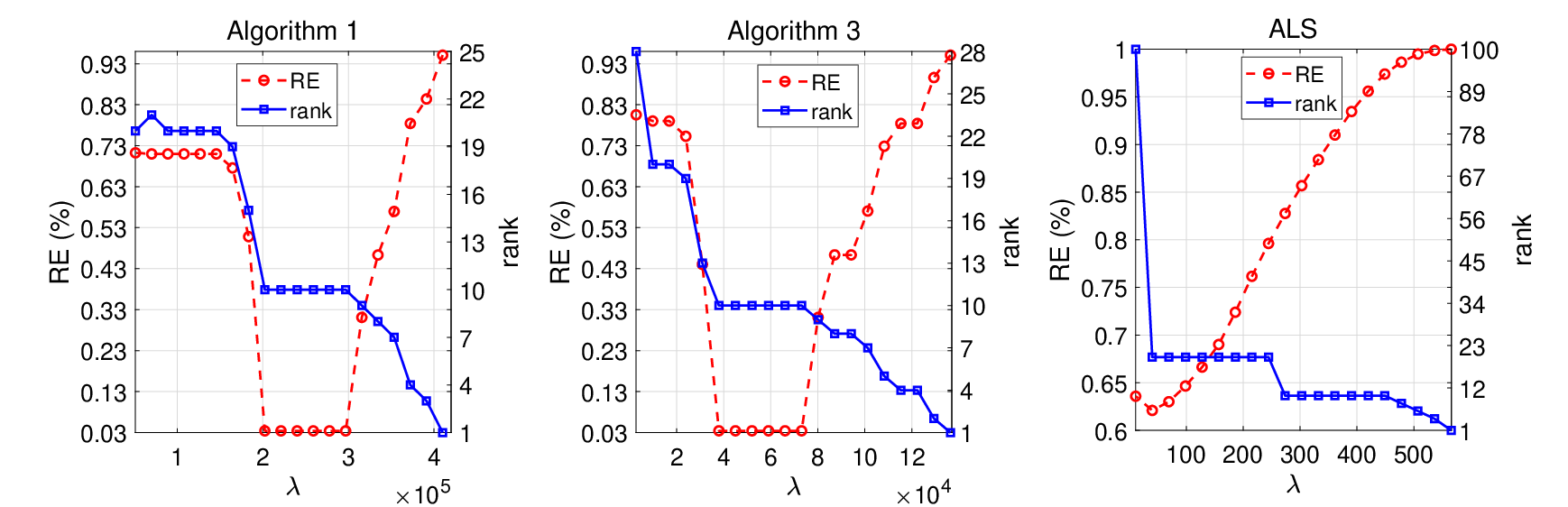
Next we present a rule to pick the best from the obtained results associated to all $\lambda_{i}$ . A desirable solution of low-rank optimization problems is expected to have a low rank and a low relative error. Since the true $M^{*}$ is unknown, the relative error is unavailable. So, in the subsequent numerical experiments, we record the loss value and rank of the output of three algorithms associated to $\lambda_{i}$ in ${\rm loss}(i)$ and ${\rm rank}(i)$ for $i=1,2,\ldots,\widehat{n}_{\lambda}$ , where $\widehat{n}_{\lambda}$ is the number of different ranks. Here, when multiple outputs have the same rank, only the one with the smallest loss value is recorded. Then we set ${\rm loss}(0)=0.5\|M_{\Omega}\|_{F}^{2}$ and ${\rm rank}(0)=0$ , and compute

\vartheta(i)=\frac{|{\rm loss}(i\!-\!1)-{\rm loss}(i)|}{|{\rm rank}(i\!-\!1)-{\rm rank}(i)|}\ \ {\rm for}\ \ i=1,2,\ldots,\widehat{n}_{\lambda}.

Clearly, $\vartheta(i)$ represents the relative change rate of the loss value with respect to the rank, obtained from model (5) associated to $\lambda_{i}$ . For the problem $\min_{U\in\mathbb{R}^{n\times r},V\in\mathbb{R}^{m\times r}}f(UV^{\mathbb{T}})$ where $f$ is the least squares loss, it is easy to verify that its optimal value has the same magnitude as the noise does when $r\geq r^{*}$ , but when $r<r^{*}$ it usually has a higher magnitude. This means that for the outputs of model (5), if their loss values have a larger change rate, it is highly possible for them to have a low rank; otherwise, they will have a high rank. Inspired by this, we find the smallest positive integer $i^{*}$ such that $\vartheta(i^{*}\!-\!1)/\vartheta(i^{*})>5$ for simulated data, and the smallest positive integer $i^{*}$ such that $\vartheta(i^{*}\!-\!1)/\vartheta(i^{*})>2$ for real data (by considering that the real data matrix usually has an approximately low rank), and then choose $\lambda_{i^{*}\!-\!1}$ as the best $\lambda$ for Algorithm 1 and ALS, and the solution associated to $\lambda_{i^{*}\!-\!1}$ yielded by Algorithm 2 as the initial point of Algorithm 3. The subsequent numerical tests always use $n_{\lambda}=21$ for three algorithms.

5.3 Numerical results for simulated data

We test four solvers on simulated data under the non-uniform sampling scheme in (29). We generate the true $M^{*}$ by $M^{*}=M_{L}^{*}(M_{R}^{*})^{\mathbb{T}}$ , where $M_{L}^{*}$ and $M_{R}^{*}$ are an $n\times r^{*}$ matrix with each entry sampled independently from the standard normal distribution $N(0,1)$ . Thus, $M^{*}\in\mathbb{R}^{n\times n}$ is a rank $r^{*}$ matrix. The noisy observation entries $M_{i_{t},j_{t}}$ with $(i_{t},j_{t})\in\Omega$ are obtained from (30) with $\sigma=0.1$ and $\xi_{t}\sim N(0,1)$ , where the index set $\Omega$ is obtained in terms of Scheme 1. To evaluate the recovery results, we adopt the metric of relative error (RE) given by $\frac{\|X^{\rm out}-M^{*}\|_{F}}{\|M^{*}\|_{F}}$ , where $X^{\rm out}$ represents the output of a solver. We consider different setting of $n,r^{*}$ and SR, and run simulation under each setting for five different instances.

Table 1: Average RE and running time of four solvers for non-uniformly sampled synthetic data

$n$	( $r^{*}$ , SR)	Algorithm 1			Algorithm 3			ALS				ADMM
		RE	rank	time(s)	RE	rank	time(s)	$c_{\lambda}$	RE	rank	time(s)	RE	rank	time(s)
1000	(8,0.10)	0.070	8	11.5	0.066	8	5.73	[0.2,10.5]	0.847	17	30.0	0.191	667	154.8
	(8,0.15)	0.046	8	15.2	0.047	8	6.79	[0.1, 7.0]	0.845	14	30.6	0.154	751	155.9
	(8,0.20)	0.038	8	15.9	0.038	8	6.86	[0.1, 5.5]	0.871	13	35.0	0.135	729	161.6
	(8,0.25)	0.032	8	19.1	0.032	8	8.44	[0.1, 4.5]	0.916	10	40.4	0.128	1000	164.2
	(10,0.10)	0.081	10	13.6	0.076	10	5.74	[0.3,10.5]	0.835	20	34.1	0.195	678	159.5
	(10,0.15)	0.052	10	16.0	0.053	10	6.79	[0.2,7.0]	0.872	16	31.7	0.160	741	157.0
	(10,0.20)	0.043	10	16.5	0.043	10	7.21	[0.1,5.5]	0.923	12	35.7	0.142	728	155.9
	(10,0.25)	0.036	10	19.8	0.036	10	8.65	[0.1,4.5]	0.817	16	40.6	0.132	1000	157.4
	(20,0.10)	0.133	20	19.6	0.129	20	6.65	[1.0, 11]	0.880	29	63.5	0.253	691	151.7
	(20,0.15)	0.084	20	18.1	0.082	20	7.57	[0.4,7.5]	0.795	33	76.1	0.187	765	151.8
	(20,0.20)	0.065	20	18.8	0.065	20	7.78	[0.2,5.5]	0.820	20	39.5	0.159	719	156.9
	(20,0.25)	0.053	20	21.2	0.054	20	9.18	[0.1,4.5]	0.883	24	49.9	0.141	1000	156.0
3000	(10,0.10)	0.039	10	105.4	0.038	10	55.8	[0.2, 10]	0.807	24	250.5	-	-	-
	(10,0.15)	0.029	10	145.1	0.028	10	65.3	[0.1,6.5]	0.870	18	220.0	-	-	-
	(10,0.20)	0.024	10	159.9	0.024	10	73.7	[0.1,5.0]	0.881	16	245.1	-	-	-
	(10,0.25)	0.020	10	260.5	0.020	10	98.2	[0.1,4.0]	0.975	10	266.4	-	-	-
	(20,0.10)	0.060	20	119.3	0.055	20	58.0	[0.3, 11]	0.973	20	203.3	-	-	-
	(20,0.15)	0.041	20	147.2	0.041	20	66.1	[0.2,7.0]	0.877	32	255.4	-	-	-
	(20,0.20)	0.034	20	172.9	0.034	20	76.0	[0.1,5.5]	0.933	24	261.5	-	-	-
	(20,0.25)	0.029	20	242.3	0.029	20	98.9	[0.1,4.0]	0.833	32	304.2	-	-	-
5000	(10,0.10)	0.030	10	318.4	0.028	10	165.5	[0.2, 11]	0.850	20	703.2	-	-	-
	(10,0.15)	0.022	10	443.4	0.022	10	200.6	[0.1,7.0]	0.706	14	759.3	-	-	-
	(10,0.20)	0.018	10	513.3	0.018	10	234.7	[0.1,5.5]	0.983	10	837.0	-	-	-
	(10,0.25)	0.016	10	913.4	0.016	10	311.0	[0.1,4.0]	0.984	10	804.4	-	-	-
	(20,0.10)	0.044	20	322.0	0.041	20	178.0	[0.3, 11]	0.934	28	639.2	-	-	-
	(20,0.15)	0.031	20	455.7	0.031	20	212.3	[0.1,7.0]	0.918	28	943.0	-	-	-
	(20,0.20)	0.026	20	546.2	0.026	20	242.9	[0.1,5.5]	0.881	32	826.2	-	-	-
	(20,0.25)	0.022	20	856.5	0.022	20	324.8	[0.1,4.0]	0.975	20	903.7	-	-	-

Table 1 reports the average RE, rank and running time (in seconds) of four solvers, where the results of ADMM are not reported for $n\geq 3000$ because it is too time-consuming. We see that for all test instances, the outputs of Algorithm 1 and 3 not only have much lower RE than those of ALS and ADMM do, but also their ranks are equal to $r^{*}$ , which coincides with their performance in Figure 2 with $\lambda$ from the best interval. This means that the proposed column $\ell_{2,0}$ -regularized factorization model is superior to another two models in capturing a low rank and low RE solution for non-uniformly sampled data. In Table 1, the columns corresponding to ADMM show that the max-norm penalized model is suitable for non-uniform sampling in terms of RE, but can not promote a low-rank solution; while the columns corresponding to ALS show that model (3) can promote low-rank solutions, but is not suitable for non-uniformly sampled data due to high RE. This coincides with the performance of the nuclear-norm and max-norm penalized models in [10].

In addition, for $r^{*}=5$ and $n=m=1000$ , Figure 3 plots the average RE over five repetitions under ${\rm SR}=0.04,0.06,0.08,\ldots,0.2$ . We see that under the two non-uniform sampling schemes, the relative errors yielded by four solvers decrease as the sampling ratio increases, but Algorithm 1 and 3 have better performance than ADMM does, and the ALS method gives the worst results.

5.4 Numerical results for real data

We test four methods with the matrix completion problem based on some real data sets, including the Jester joke dataset, the MovieLens dataset, and the Netflix dataset. For each data set, let $M^{0}$ be the original incomplete data matrix such that the $i$ th row of $M^{0}$ corresponds to the ratings given by the $i$ th user. We first consider the Jester joke dataset which is available through http://www.ieor.berkeley.edu/~goldberg/jester-data/. This dataset contains more than 4.1 million ratings for $100$ jokes from $73,421$ users. The whole Jester joke dataset contains three subdatasets: (1) jester-1: 24,983 users who rate 36 or more jokes; (2) jester-2: 23,500 users who rate 36 or more jokes; (3) jester-3: 24,938 users who rate between 15 and 35 jokes. More descriptions can be found in [7, 23, 37], where the nuclear-norm convex relaxation is used to study this dataset. Due to the large number of users, we first randomly select $n_{u}$ rows from $M^{0}$ and then randomly permute the ratings from these users to generate $M\in\mathbb{R}^{{n_{u}}\times 100}$ as in [10]. Next, we adopt Scheme 1 to generate a set $\Omega$ of observed indices. Since we can only observe the entry $(j,k)$ if $(j,k)\in\Omega$ and $M_{jk}$ is given, the actual sampling ratio is less than the input SR.

Since the true $M^{*}$ is unknown for real datasets, we cannot compute the relative error as we did for simulated data. Similar to [37], we use the metric of the normalized mean absolute error

{\rm NMAE}=\frac{\sum_{(i,j)\in\Gamma\backslash\Omega}|X^{\rm out}_{i,j}-M_{i,j}|}{|\Gamma\backslash\Omega|(r_{\rm max}-r_{\rm min})}

to measure the accuracy of the output of an algorithm, where $\Gamma\!:=\{(i,j)\in[n_{u}]\times[100]\!:M_{ij}\ \textrm{is given}\}$ denotes the set of indices for which $M_{ij}$ is given, and $r_{\rm min}$ and $r_{\rm max}$ denote the lower and upper bounds for the ratings, respectively. In the Jester joke dataset, the range is from $-10$ to $10$ .

Table 2: Average NMAE and running time of four solvers for the Jester joke dataset

Dataset	( $n_{u}$ , SR)	Algorithm 1			Algorithm 3			ALS				ADMM
		NMAE	rank	time	NMAE	rank	time	$\ \ \ \ c_{\lambda}$	NMAE	rank	time	NMAE	rank	time
jester-1	(1000,0.15)	0.228	9	2.01	0.198	1	0.29	[0.9,6.4]	0.217	6	6.62	0.195	100	25.3
	(1000,0.20)	0.188	1	0.33	0.188	1	0.20	[0.8,4.8]	0.221	1	1.46	0.190	100	25.2
	(1000,0.25)	0.187	1	0.21	0.187	1	0.16	[0.8,3.6]	0.223	1	0.82	0.188	100	25.2
	(2000,0.15)	0.195	1	0.82	0.195	1	0.48	[1.2,6.0]	0.221	1	1.79	0.196	100	177.3
	(2000,0.20)	0.194	1	0.58	0.194	1	0.43	[1.0,4.8]	0.222	1	3.10	0.193	100	176.4
	(2000,0.25)	0.189	1	0.50	0.189	1	0.39	[0.9,3.8]	0.221	1	3.16	0.189	100	176.1
	(4000,0.15)	0.203	8	7.46	0.196	1	1.37	[1.4,6.4]	0.222	2	6.82	-	-	-
	(4000,0.20)	0.190	1	1.22	0.190	1	0.88	[1.0,4.6]	0.222	1	2.74	-	-	-
	(4000,0.25)	0.185	1	1.41	0.185	1	0.88	[0.9,3.8]	0.222	1	7.99	-	-	-
jester-2	(1000,0.15)	0.197	1	0.29	0.196	1	0.21	[0.9,6.2]	0.217	8	6.35	0.196	100	24.1
	(1000,0.20)	0.189	1	0.20	0.189	1	0.14	[0.8,4.6]	0.223	1	0.82	0.192	100	24.2
	(1000,0.25)	0.187	1	0.20	0.187	1	0.15	[0.8,3.6]	0.224	1	0.72	0.190	100	24.2
	(2000,0.15)	0.196	1	0.71	0.194	1	0.69	[1.3,6.4]	0.223	1	3.49	0.195	100	178.9
	(2000,0.20)	0.189	1	1.02	0.189	1	0.53	[1.0,4.8]	0.222	1	3.29	0.192	100	177.2
	(2000,0.25)	0.188	1	0.49	0.188	1	0.37	[0.8,3.8]	0.219	4	7.42	0.190	100	177.6
	(4000,0.15)	0.194	1	1.22	0.194	1	0.80	[1.3,6.4]	0.222	2	7.66	-	-	-
	(4000,0.20)	0.187	1	0.86	0.187	1	0.66	[1.0,4.6]	0.222	1	3.46	-	-	-
	(4000,0.25)	0.186	1	0.84	0.186	1	0.64	[0.9,3.4]	0.223	1	2.96	-	-	-
jester-3	(1000,0.15)	0.276	3	1.34	0.259	2	0.43	[0.1,6.8]	0.227	11	6.08	0.217	88	23.8
	(1000,0.20)	0.251	1	0.44	0.244	4	0.27	[0.1,4.8]	0.227	4	5.28	0.212	87	24.2
	(1000,0.25)	0.301	5	2.33	0.263	2	0.25	[0.1,4.4]	0.227	8	7.18	0.213	91	24.2
	(2000,0.15)	0.245	3	6.91	0.241	4	1.30	[0.1,7.2]	0.227	10	13.5	0.217	91	173.9
	(2000,0.20)	0.258	6	9.85	0.248	5	1.52	[0.1,5.0]	0.223	8	17.0	0.212	91	176.1
	(2000,0.25)	0.268	3	5.84	0.252	2	1.16	[0.2,4.0]	0.224	12	20.9	0.213	91	177.8
	(4000,0.15)	0.249	1	4.97	0.245	2	1.65	[0.3,7.0]	0.229	5	21.6	-	-	-
	(4000,0.20)	0.258	2	6.53	0.255	2	2.04	[0.3,5.2]	0.231	3	11.3	-	-	-
	(4000,0.25)	0.234	2	4.64	0.241	2	1.89	[0.3,4.0]	0.226	8	21.7	-	-	-

For the Jester joke dataset, we consider different settings of $n_{u}$ and SR, and report the average NMAE, rank and time (in seconds) for running the same setting five times in Table 2. Among others, the results of ADMM for $n_{u}=4000$ are not reported since the adjusting scheme of $\lambda$ is not available in the code. We see that for jester-1 and jester-2, Algorithm 1 and 3 yield comparable even a little better NMAE than ADMM does, but for jester-3 they give a little worse NMAE than ALS and ADMM do. For all settings, Algorithm 1 and 3 yield much lower rank and require much less running time than ADMM does. The ALS method yields the worst NMAE for jester-1 and jester-2, and require comparable running time with that of Algorithm 1 and 3.

Next we consider the MovieLens dataset from http://www.grouplens.org/node/73. The dataset contains two subdatasets: the Movie-100K dataset and the Movie-1M dataset, and the rating range is from $r_{\rm min}=1$ to $r_{\rm max}=5$ . The Movie-100K dataset contains 100,000 ratings for 1682 movies by 943 users, while the latter contains 1,000,209 ratings of 3900 movies made by 6040 users. For the Movie-100K dataset, we also consider the data matrix $\widetilde{M}^{0}=M^{0}-3$ so as to be consistent with the code of ADMM. We first randomly select $n_{r}$ users from $\widetilde{M}^{0}$ and randomly select their $n_{c}$ column ratings, and then sample the observed entries with the schemes in (29). Table 3 reports the averaged NMAE, rank and running time (in seconds) after running the setting $(n_{r},n_{c})=(943,1682)$ five times. We see that Algorithm 3 yields a little better NMAE than other three solvers do, Algorithm 1 gives worse NMAE than ADMM does for ${\rm SR}=0.1$ and $0.15$ ; and Algorithm 1 and 3 yield the lowest rank solutions for all test problems, but ADMM gives the highest rank solutions.

Table 3: Average NMAE and running time of four methods for Movie-100K dataset

	SR	Algorithm 1			Algorithm 3			ALS				ADMM
		NMAE	rank	time	NMAE	rank	time	$c_{\lambda}$	NMAE	rank	time	NMAE	rank	time
Scheme 1	0.10	0.244	1	15.5	0.231	1	2.93	[0.4,9.2]	0.248	10	18.8	0.232	757	354.3
	0.15	0.226	1	16.9	0.219	1	3.08	[0.4,5.4]	0.247	1	3.63	0.225	867	353.9
	0.20	0.216	1	16.3	0.212	1	3.37	[0.3,5.0]	0.244	5	23.1	0.220	901	361.8
	0.25	0.209	1	17.6	0.207	1	3.59	[0.3,2.6]	0.242	1	5.56	0.215	927	361.8
Scheme 2	0.10	0.246	1	15.3	0.232	1	2.90	[0.3,9.2]	0.248	5	12.5	0.233	752	360.9
	0.15	0.229	1	18.1	0.221	1	3.05	[0.3,6.2]	0.247	12	19.2	0.226	851	361.6
	0.20	0.217	1	17.0	0.212	1	3.33	[0.3,5.0]	0.244	10	21.2	0.221	900	369.0
	0.25	0.210	1	15.4	0.208	1	3.39	[0.3,2.6]	0.244	1	4.93	0.217	922	366.7

Table 4: Average NMAE and running time of four methods for Movie-1M dataset

( $n_{r}$ , $n_{c}$ )	SR	Algorithm 1			Algorithm 3			ALS				ADMM
		NMAE	rank	time	NMAE	rank	time	$c_{\lambda}$	NMAE	rank	time	NMAE	rank	time
$1500\times 1500$	0.10	0.242	1	22.8	0.229	1	4.41	[0.5,8.2]	0.251	1	6.50	0.234	850	525.3
	0.15	0.226	1	25.4	0.218	1	4.44	[0.4,5.2]	0.250	1	6.55	0.227	999	527.4
	0.20	0.212	1	24.4	0.209	1	4.49	[0.3,3.4]	0.249	1	6.07	0.221	1100	532.0
	0.25	0.207	1	29.7	0.205	1	4.85	[0.3,3.0]	0.247	1	7.65	0.217	1156	534.5
$2000\times 2000$	0.10	0.228	1	41.5	0.219	1	8.11	[0.8,9.4]	0.251	3	21.4	0.231	1245	1263.1
	0.15	0.212	1	53.1	0.209	1	8.52	[0.6,4.8]	0.251	1	10.9	0.223	1415	1271.9
	0.20	0.207	1	44.1	0.204	1	8.70	[0.5,3.8]	0.250	1	9.59	0.219	1524	1275.9
	0.25	0.201	1	39.5	0.200	1	9.70	[0.3,2.4]	0.248	1	12.8	0.213	1602	1363.3
$3000\times 3000$	0.10	0.216	1	107.5	0.210	1	23.9	[1.2,7.8]	0.253	1	22.8	-	-	-
	0.15	0.204	1	104.8	0.202	1	23.4	[0.8,4.4]	0.249	1	25.7	-	-	-
	0.20	0.199	1	79.3	0.197	1	24.2	[0.6,3.2]	0.248	1	25.4	-	-	-
	0.25	0.195	1	81.4	0.195	1	28.0	[0.4,2.2]	0.242	1	29.1	-	-	-
$6040\times 3706$	0.10	0.205	1	274.9	0.202	1	56.9	[1.3,6.8]	0.251	1	50.1	-	-	-
	0.15	0.197	1	218.2	0.196	1	60.8	[0.8,4.2]	0.248	1	58.5	-	-	-
	0.20	0.194	1	174.5	0.194	1	61.1	[0.6,3.2]	0.247	1	54.8	-	-	-
	0.25	0.192	1	177.1	0.192	1	64.0	[0.4,2.4]	0.245	1	71.1	-	-	-

For the Movie-1M dataset, we first randomly select $n_{r}$ users and their $n_{c}$ column ratings from $M^{0}$ , and then sample the observed entries with Scheme 1 in (29). We consider the setting of $n_{r}=n_{c}$ with $n_{r}=1500,2000$ or $3000$ and the setting of $(n_{r},n_{c})=(6040,3706)$ . Table 4 reports the average NMAE, rank and running time (in seconds) after running five times for each setting. We see that for this dataset, the solvers have similar performance as they do for the Movie-100K.

Table 5: Average NMAE and running time of three methods for Netflix Dataset

	( $n_{r}$ , $n_{c}$ )	SR	Algorithm 1			Algorithm 3			ALS
			NMAE	rank	time	NMAE	rank	time	$c_{\lambda}$	NMAE	rank	time
scheme 1	$6000\times 6000$	0.10	0.228	1	440.1	0.218	1	121.4	[1.1,8.4]	0.246	1	110.1
		0.15	0.214	1	460.3	0.209	1	125.9	[0.8,5.2]	0.243	1	111.6
		0.20	0.208	1	496.6	0.204	1	127.4	[0.6,3.4]	0.244	1	113.9
		0.25	0.203	1	452.1	0.201	1	133.2	[0.5,3.0]	0.242	1	127.9
	$8000\times 8000$	0.10	0.214	1	726.4	0.208	1	140.7	[1.3,9.0]	0.246	1	106.5
		0.15	0.206	1	762.0	0.203	1	148.5	[0.8,5.4]	0.244	1	104.4
		0.20	0.201	1	824.4	0.199	1	152.5	[0.6,3.6]	0.244	1	126.4
		0.25	0.198	1	760.4	0.196	1	163.4	[0.5,2.8]	0.241	1	130.6
	$10000\times 10000$	0.10	-	-	-	0.207	1	217.3	[1.4,8.2]	0.245	1	170.8
		0.15	-	-	-	0.200	1	241.1	[0.9,5.6]	0.244	1	158.1
		0.20	-	-	-	0.198	1	243.9	[0.7,3.8]	0.245	1	176.2
		0.25	-	-	-	0.195	1	265.2	[0.5,2.8]	0.242	1	191.4
scheme 2	$6000\times 6000$	0.10	0.229	1	395.2	0.219	1	78.3	[1.0,8.4]	0.246	1	63.8
		0.15	0.216	1	433.1	0.209	1	79.9	[0.8,5.6]	0.244	1	63.4
		0.20	0.208	1	452.7	0.204	1	83.5	[0.6,3.6]	0.245	1	69.0
		0.25	0.204	1	421.9	0.201	1	84.0	[0.4,3.0]	0.243	1	83.0
	$8000\times 8000$	0.10	0.214	1	714.5	0.209	1	141.2	[1.2,9.0]	0.246	1	102.8
		0.15	0.206	1	712.8	0.203	1	146.8	[0.8,5.4]	0.245	1	103.1
		0.20	0.201	1	803.2	0.199	1	152.1	[0.6,3.6]	0.244	1	114.4
		0.25	0.198	2	763.6	0.197	1	155.7	[0.4,2.8]	0.241	1	98.0

We also consider the Netflix dataset in https://www.kaggle.com/netflix-inc/netflix-prize-data#qualifying.txt. For this dataset, we first randomly select $n_{r}$ users and their $n_{c}$ column ratings from $M^{0}$ , and then sample the observed entries with the schemes in (29). We consider the setting of $n_{r}=n_{c}$ with $n_{r}=6000,8000$ and $10000$ . Table 5 reports the average NMAE, rank and running time (in seconds) of three solvers after running five times for each setting (the results of ADMM are not reported for these instances since it is too time-consuming). For this dataset, the three solvers have similar performance as they do for the MovieLens dataset. Among others, Algorithm 3 yields better outputs than other two solvers do, and it requires less half of the time than Algorithm 1 does. So, Algorithm 3 has a remarkable advantage in running time for large-scale instances.

From the numerical tests of the previous two subsections, we conclude that for simulated data, Algorithm 1 and 3 are superior to ALS and ADMM in terms of rank and relative error; and for the three real datasets, Algorithm 3 is superior to other three solvers in terms of rank and NMAE except for jester-3, and its running time is also comparable with that of ALS.

6 Conclusion

We have proposed a column $\ell_{2,0}$ -norm regularized factorization model for low-rank matrix recovery to achieve the optimal (or true) rank from a rough upper estimation, so that the recent theoretical results for factorization models work fully in practice. We verify from theory that this model is superior to the squared Frobenius-norm regularized model (3); for example, the critical points of model (5) associated to a suitable $\lambda$ and a tiny $\mu$ will have rank $r^{*}$ if their objective values are not greater than that of the projection of the noisy observation onto the rank $r^{*}$ -constraint set, and under a suitable condition on $f$ , the solution associated to a local minimizer of model (5) with rank $r^{*}$ has a better error bound to the true $M^{*}$ than the solution associated to a local minimizer of model (3) with rank $r^{*}$ does. We have developed an AMM method and a hybrid AMM method for computing this model, and provided their global convergence analysis. Numerical experiments are conducted on simulated data and real datasets for matrix completion problem with non-uniform sampling, and comparison results with the ALS [14] and the ADMM [10] show that the proposed model has an advantage in promoting solutions with lower errors and ranks, and the hybrid AMM method is superior to other three solvers for most of test instances in terms of the error, rank and running time. The interesting future work is about the statistical study on the proposed model.

Acknowledgements The authors would like to express their sincere thanks to Prof. Ethan X. Fang from Pennsylvania State University for providing them with the ADMM code for numerical comparison. The authors would like to express their sincere thanks to two anonymous referees and the Associated Editor for their helpful comments.

References

[1] H. Attouch, J. Bolte, P. Redont and A. Soubeyran, Proximal alternating minimization and projection methods for nonconvex problems: an approach based on the Kurdyka-Łojasiewicz inequality, Mathematics of Operations Research, 35(2010), pp. 438–457.
[2] S. Bhojanapalli, B. Neyshabur and N. srebro, Global optimality of local search for low rank matrix recovery, Advances in Neural Information Processing Systems, 29(2016), pp. 3873–3881.
[3] J. Bolte, S. Sabach and M. Teboulle, Proximal alternating linearized minimization for nonconvex and nonsmooth problems, Mathematical Programming, 146(2014), pp. 459–494.
[4] S. Burer and R. D. Monteiro, A nonlinear programming algorithm for solving semidefinite programs with low-rank factorization, Mathematical Programming, 95(2003), pp. 329–357.
[5] E. J. Candès and B. Recht, Exact matrix completion via convex optimization, Foundations of Computational Mathematics, 9(2009), pp. 717–772.
[6] E. J. Candès and Y. Plain, Tight oracle inequalities for low-rank matrix recovery from a minimal number of noisy random measurements, IEEE Transactions on Information Theory, 57(2011), pp. 2342–2359.
[7] C. H. Chen, B. S. He and X. M. Yuan, Matrix completion via an alternating direction method, IMA Journal of Numerical Analysis, 32(2012), pp. 227–245.
[8] J. Chi, R. Ge, P. Netrapalli, S. M. Kakade and M. I. Jordan, How to escape saddle points efficiently, Proceedings of the 34th International Conference on Machine Learning, 70(2017), pp. 1724–1732.
[9] M. A. Davenport and J. Romberg, An overview of low-rank matrix recovery from incomplete observations, IEEE Journal of Selected Topics in Signal Processing, 10(2016), pp. 608–622.
[10] E. X. Fang, H. Liu, K. C. Toh and W. X. Zhou, Max-norm optimization for robust matrix recovery, Mathematical Programming, 167(2018), pp. 5–35.
[11] M. Fazel, Matrix rank minimization with applications, PhD thesis, Stanford University, 2002.
[12] R. Ge, C. Jin and Y. Zheng, No spurious local minima in nonconvex low rank problems: A unified geometric analysis, Proceedings of the 34th International Conference on Machine Learning, 70(2017), pp. 1233–1242.
[13] D. Gross, Y. K. Liu, S. T. Flammia, S. Becker and J. Eisert, Quantum state tomography via compressed sensing, Physical Review Letters, 105(2010), pp. 1–4.
[14] T. Hastie, R. Mazumder, J. D. Lee and R. Zadeh, Matrix completion and low-rank SVD via fast alternating least squares, Journal of Machine Learning Research, 16(2015), pp. 3367–3402.
[15] P. Jain, P. Netrapalli and S. Sanghavi, Low-rank matrix completion using alternating minimization, In Proceedings of the 45th annual ACM Symposium on Theory of Computing, 2013, pp. 665–674.
[16] J. Lee, B. Recht, R. Salakhutdinov, N. Srebro and J. Tropp, Practical large-scale optimization for max-norm regularization, Advances in Neural Information Processing Systems, 1(2010), pp. 1297–1305.
[17] J. D. Lee, I. Panageas, G. Piliouras, M. Simchowitz, M. I. Jordan and B. Recht, First-order methods almost always avoid strict saddle points, Mathematical Programming, 176(2019), pp. 311–337.
[18] X. G. Li, J. W. Lu, R. Arora, J. Haupt, H. Liu, Z. R. Wang and T. Zhao, Symmetry, saddle points, and global optimization landscape of nonconvex matrix factorization, IEEE Transactions on Information Theory, 65(2019), pp. 3489–3514.
[19] Q. W. Li, Z. H. Zhu and G. G. Tang, The non-convex geometry of low-rank matrix optimization, Information and Inference: A Journal of the IMA, 8(2018), pp. 51–96.
[20] T. X. Liu, T. K. Pong and A. Takeda, A refined convergence analysis of pDCA_e with applications to simultatneous sparse recovery and outlier detection, Computation Optimization and Applications, 73(2019), pp. 69–100.
[21] Z. S. Lu and Y. Zhang, Sparse approximation via penalty decomposition methods, SIAM Journal on Optimization, 23(2013), pp. 2448–2478.
[22] Z. S. Lu, Iterative hard thresholding methods for $l_{0}$ regularized convex cone programming, Mathematical Programming, 147(2014), pp. 125–154.
[23] S. Q. Ma, D. Goldfarb and L. F. Chen, Fixed point and Bregman iterative methods for matrix rank minimization, Mathematical Programming, 128(2009), pp. 321–353.
[24] S. Negahban and M. J. Wainwright, Estimation of (near) low-rank matrices with noise and high-dimensional scaling, The Annals of Statistics, 39(2011), pp. 1069–1097.
[25] S. Negahban and M. J. Wainwright, Restricted strong convexity and weighted matrix completion: optimal bounds with noise, Journal of Machine Learning Research, 13(2012), pp. 1665–1697.
[26] Y. Nesterov, A method of solving a convex programming problem with convergence rate $O(1/k^{2})$ , Soviet Mathematics Doklady, 27(1983), pp. 372–376.
[27] D. Park, A. Kyrillidis, C. Caramanis and S. Sanghavi, Finding low-rank solution via non-convex matrix factorization efficiently and provably, SIAM Journal on Imaging Sciences, 11(2018), pp. 2165–2204.
[28] D. Park, A. Kyrillidis, C. Caramanis and S. Sanghavi, Non-square matrix sensing without spurious local minima via the Burer-Monteiro approach, In Proceedings of the 20th International Conference on Artificial Intelligence and Statistics, 54(2017), pp. 65–74.
[29] T. Pock and S. Sabach, Inertial proximal alternating linearized minimization (iPALM) for nonconvex and nonsmooth problems, SIAM Journal on Imaging Sciences, 9(2016), pp. 1756–1787.
[30] B. Recht, M. Fazel and P. A. Parrilo, Guaranteed minimum-rank solutions of linear matrix equations via nuclear norm minimization, SIAM Review, 52(2010), pp. 471–501.
[31] R. T. Rockafellar and R. J-B. Wets, Variational analysis, Springer, 1998.
[32] F. H. Shang, Y. Y. Liu and J. Cheng, Tractable and scalable schatten quasi-norm approximations for rank minimization, Proceedings of the 19th International Conference on Artificial Intelligence and Statistics, 51(2016), pp. 620–629.
[33] N. Srebro, J. D. M. Rennie and T. Jaakkola, Maximum-margin matrix factorization, Advances in Neural Information Processing Systems, 2005, pp. 1329-1336.
[34] N. Srebro and R. R. Salakhutdinov, Collaborative filtering in a non-uniform world: learning with the weighted trace norm, Advances in Neural Information Processing Systems, 2(2010), pp. 2056–2064.
[35] R. Y. Sun and Z. Q. Luo, Guaranteed matrix completion via non-convex factorization, IEEE Transactions on Information Theory, 62(2016), pp. 6535–6579.
[36] S. Tu, R. Boczar, M. Simchowitz, M. Soltanolkotabi and B. Recht, Low-rank solution of linear matrix equations via procrustes flow, In International Conference on Machine Learning, 48(2016), pp. 964–973.
[37] K. C. Toh and S. Yun, An accelerated proximal gradient algorithm for nuclear norm regularized linear least squares problems, Pacific Journal of Optimization, 6(2010), pp. 615–640.
[38] T. Tao, S. H. Pan and S. J. Bi, Error bound of critical points and KL property of exponent $1/2$ for squared F-norm regularized factorization, Journal of Global Optimization, 81(2021), pp. 991–1017.
[39] Z. W. Wen, W. T. Yin and Y. Zhang, Solving a low-rank factorization model for matrix completion by a nonlinear successive over-relaxation algorithm, Mathematical Programming Computation, 4(2012), pp. 333–361
[40] Y. Y. Xu and W. T. Yin, A globally convergent algorithm for nonconvex optimization based on block coordinate update, Journal of Scientific Computing, 72(2017), pp. 700–734.
[41] L. Yang, T. K. Pong and X. J. Chen, A nonmonotone alternating updating method for a class of matrix factorization problems, SIAM Journal on Optimization, 28(2018), pp. 3402–3430.
[42] Q. Zhang, C. H. Chen, H. K. Liu and A. M. C. So, On the linear convergence of the ADMM for regularized non-convex low-rank matrix recovery, https://www1.se.cuhk.edu.hk/~manchoso/admm_MF.pdf, 2018.
[43] Q. Zheng and J. Lafferty, A convergent gradient descent algorithm for rank minimization and semidefinite programming from random linear measurements, Advances in Neural Information Processing Systems, 1(2015), pp. 109–117.
[44] Z. H. Zhu, Q. W. Li, G. G. Tang and M. B. Wakin, Global optimization in low-rank matrix optimization, IEEE Transactions on Signal Processing, 66(2018), pp. 3614–3628.
[45] X. W. Zhou, C. Yang, H. Y. Zhao and W. C. Yu, Low-rank modeling and its applications in image analysis, ACM Computing Surveys, 47(2015), pp. 1–33.

Appendix A:

This part provides a lower bound to $M^{*}$ for the solution associated to a critical point of $F_{\lambda}$ .

Proposition 1.

Let $f(X)\!:=h(\mathcal{A}(X)-b)$ where $h\!:\mathbb{R}^{p}\to\mathbb{R}$ is an $L_{h}$ -smooth function, $\mathcal{A}\!:\mathbb{R}^{n\times m}\to\mathbb{R}^{p}$ is the sampling operator, and $b=\mathcal{A}(M^{*})+\omega$ for a noise vector $\omega\in\mathbb{R}^{p}$ . Then, for any nonzero $(\overline{U},\overline{V})\in{\rm crit}F_{\lambda}$ , it holds that $\|\overline{U}\overline{V}^{\mathbb{T}}\!-M^{*}\|_{F}\geq\max\big(0,\frac{\lambda-\|\mathcal{A}^{*}\nabla h(\omega)\|}{L_{h}\|\mathcal{A}\|^{2}}\big).$

Proof.

Fix any nonzero $(\overline{U},\overline{V})\in{\rm crit}F_{\lambda}$ . By the expression of $F_{\lambda}$ , it is immediate to have that $\nabla\!f(\overline{U}\overline{V}^{\mathbb{T}})\overline{V}+\lambda\overline{U}=0$ and $[\nabla\!f(\overline{U}\overline{V}^{\mathbb{T}})]^{\mathbb{T}}\overline{U}+\lambda\overline{V}=0$ . Then, it holds that

\langle\overline{U},\nabla\!f(\overline{U}\overline{V}^{\mathbb{T}})\overline{V}+\lambda\overline{U}\rangle=0\ \ {\rm and}\ \ \langle\overline{V},\big[\nabla\!f(\overline{U}\overline{V}^{\mathbb{T}})\big]^{\mathbb{T}}\overline{U}+\lambda\overline{V}\rangle=0.

Recall that $\overline{U}^{\mathbb{T}}\overline{U}=\overline{V}^{\mathbb{T}}\overline{V}$ (see [19, Proposition 4.3]). Together with the last two equalities, we obtain

-\lambda\|\overline{U}\|_{F}^{2}=\langle\overline{U},\nabla\!f(\overline{U}\overline{V}^{\mathbb{T}})\overline{V}\rangle\geq-\|\overline{U}\overline{V}^{\mathbb{T}}\|_{*}\|\nabla\!f(\overline{U}\overline{V}^{\mathbb{T}})\|\geq-\|\overline{U}\|_{F}^{2}\|\nabla\!f(\overline{U}\overline{V}^{\mathbb{T}})\|,

where the last inequality is since $\|X\|_{*}=\displaystyle{\min_{U\in\mathbb{R}^{n\times r},V\in\mathbb{R}^{m\times r}}}\big\{\frac{1}{2}(\|U\|_{F}^{2}+\|V\|_{F}^{2})\ {\rm s.t.}\ X=UV^{\mathbb{T}}\big\}.$ Note that $\overline{U}\neq 0$ and $\overline{V}\neq 0$ since $(\overline{U},\overline{V})$ is nonzero and $\overline{U}^{\mathbb{T}}\overline{U}=\overline{V}^{\mathbb{T}}\overline{V}$ . From the last inequality, it follows that $\|\nabla\!f(\overline{U}\overline{V}^{\mathbb{T}})\|\geq\lambda$ . Substituting $\nabla\!f(X)=\mathcal{A}^{*}\nabla h(\mathcal{A}(X)-b)$ into this inequality and using the Lipschitz continuity of $\nabla h$ yields that $\lambda\leq L_{h}\|\mathcal{A}\|^{2}\|\overline{U}\overline{V}^{\mathbb{T}}\!-M^{*}\|_{F}+\|\mathcal{A}^{*}\nabla h(\omega)\|.$ This implies that the desired inequality holds. The proof is completed.

Note that a suitably large $\lambda$ is necessary for model (3) to achieve a solution with rank close to $r^{*}$ if the upper estimation $r$ is too rough. Together with the lower bound in Proposition 1, such $\lambda$ will lead to a large error bound to the true $M^{*}$ for the solution corresponding to the critical point of (3). Thus, it is very hard to achieve a solution with a small error and a rank close to the true $r^{*}$ by solving model (3). The last subfigure in Figure 2 precisely shows this phenomenon.

Appendix B: The proof of Proposition 3.2.

Proof: By the optimality of $U^{k+1}$ and the feasibility of $U^{k}$ to (11), it follows that

		$\displaystyle\langle\nabla_{\!1}F(\widetilde{U}^{k},V^{k}),U^{k+1}\rangle+\frac{\mu}{2}\\|U^{k+1}\\|_{F}^{2}+\frac{\gamma_{1,k}}{2}\\|U^{k+1}\!-\!\widetilde{U}^{k}\\|_{F}^{2}+\lambda\\|U^{k+1}\\|_{2,0}$
		$\displaystyle\leq\langle\nabla_{\!1}F(\widetilde{U}^{k},V^{k}),U^{k}\rangle+\frac{\mu}{2}\\|U^{k}\\|_{F}^{2}+\frac{\gamma_{1,k}}{2}\\|U^{k}\!-\!\widetilde{U}^{k}\\|_{F}^{2}+\lambda\\|U^{k}\\|_{2,0}.$		(33)

By invoking inequality (9a) with $\gamma=\gamma_{1,k},V=V^{k},U^{\prime}=U^{k+1}$ and $U=\widetilde{U}^{k}$ , we obtain

		$\displaystyle F(U^{k+1},V^{k})\leq F(\widetilde{U}^{k},V^{k})+\langle\nabla_{\!1}F(\widetilde{U}^{k},V^{k}),U^{k+1}\!-\!\widetilde{U}^{k}\rangle+\frac{\tau_{V^{k}}}{2}\\|U^{k+1}\!-\!\widetilde{U}^{k}\\|_{F}^{2}$
		$\displaystyle\leq F(U^{k},V^{k})+\langle\nabla_{\!1}F(\widetilde{U}^{k},V^{k}),U^{k+1}-U^{k}\rangle+\frac{\tau_{V^{k}}}{2}\\|U^{k}\!-\!\widetilde{U}^{k}\\|_{F}^{2}+\frac{\tau_{V^{k}}}{2}\\|U^{k+1}\!-\!\widetilde{U}^{k}\\|_{F}^{2}$		(34)

where the last inequality is by (9b) with $\gamma=\tau_{V^{k}},V=\!V^{k},U=\!\widetilde{U}^{k}$ and $U^{\prime}=U^{k}$ . Along with (Column $\ell_{2,0}$ -norm regularized factorization model of low-rank matrix recovery and its computation),

	$\displaystyle F(U^{k+1},V^{k})$	$\displaystyle\leq F(U^{k},V^{k})+\frac{\mu}{2}\\|U^{k}\\|_{F}^{2}+\lambda\\|U^{k}\\|_{2,0}+\frac{\gamma_{1,k}+\tau_{V^{k}}}{2}\\|U^{k}\!-\!\widetilde{U}^{k}\\|_{F}^{2}$
		$\displaystyle\quad-\frac{\gamma_{1,k}-\tau_{V^{k}}}{2}\\|U^{k+1}\!-\!\widetilde{U}^{k}\\|_{F}^{2}-\frac{\mu}{2}\\|U^{k+1}\\|_{F}^{2}-\lambda\\|U^{k+1}\\|_{2,0}.$		(35)

By using the same arguments as those for (Column $\ell_{2,0}$ -norm regularized factorization model of low-rank matrix recovery and its computation) and the optimality of $V^{k+1}$ to (12), it follows that

	$\displaystyle F(U^{k+1},V^{k+1})$	$\displaystyle\leq F(U^{k+1},V^{k})+\frac{\mu}{2}\\|V^{k}\\|_{F}^{2}+\lambda\\|V^{k}\\|_{2,0}-\frac{\mu}{2}\\|V^{k+1}\\|_{F}^{2}-\lambda\\|V^{k+1}\\|_{2,0}$
		$\displaystyle\quad+\frac{\gamma_{2,k}+\tau_{U^{k+1}}}{2}\\|V^{k}\!-\!\widetilde{V}^{k}\\|_{F}^{2}-\frac{\gamma_{2,k}-\tau_{U^{k+1}}}{2}\\|V^{k+1}\!-\!\widetilde{V}^{k}\\|_{F}^{2}.$		(36)

By substituting (Column $\ell_{2,0}$ -norm regularized factorization model of low-rank matrix recovery and its computation) into this inequality and using the definition of $\Phi_{\lambda,\mu}$ , it follows that

	$\displaystyle\Phi_{\lambda,\mu}(U^{k+1},V^{k+1})$	$\displaystyle\leq\Phi_{\lambda,\mu}(U^{k},V^{k})+\frac{\gamma_{1,k}+\tau_{V^{k}}}{2}\\|U^{k}\!-\!\widetilde{U}^{k}\\|_{F}^{2}+\frac{\gamma_{2,k}+\tau_{U^{k+1}}}{2}\\|V^{k}\!-\!\widetilde{V}^{k}\\|_{F}^{2}$
		$\displaystyle\quad-\frac{\gamma_{1,k}-\tau_{V^{k}}}{2}\\|U^{k+1}\!-\!\widetilde{U}^{k}\\|_{F}^{2}-\frac{\gamma_{2,k}-\tau_{U^{k+1}}}{2}\\|V^{k+1}\!-\!\widetilde{V}^{k}\\|_{F}^{2}.$		(37)

Together with $\widetilde{U}^{k}=U^{k}+\beta_{k}(U^{k}-U^{k-1})$ and $\widetilde{V}^{k}=V^{k}+\beta_{k}(V^{k}\!-\!V^{k-1})$ and the definitions of $\alpha_{1,k}$ and $\alpha_{2,k}$ , we deduce that for each integer $k\geq 0$ the left hand side of (3.2) is not more than

	$\displaystyle{\rm RHT}$	$\displaystyle=\frac{2\tau_{V^{k}}\beta_{k}^{2}-\rho_{1}\alpha_{1,k}}{2}\big\\|U^{k}\!-\!U^{k-1}\big\\|_{F}^{2}-\frac{(1-\rho_{1})(\gamma_{1,k}-\tau_{V^{k}})}{2}\big\\|U^{k+1}\!-\!U^{k}\big\\|_{F}^{2}$
		$\displaystyle\quad+(\gamma_{1,k}\!-\!\tau_{V^{k}})\beta_{k}\langle U^{k+1}\!-\!U^{k},U^{k}\!-\!U^{k-1}\rangle+(\gamma_{2,k}\!-\!\tau_{U^{k+1}})\beta_{k}\langle V^{k+1}\!-\!V^{k},V^{k}\!-\!V^{k-1}\rangle$
		$\displaystyle\quad+\frac{2\tau_{U^{k+1}}\beta_{k}^{2}-\rho_{2}\alpha_{2,k}}{2}\\|V^{k}\!-\!V^{k-1}\\|_{F}^{2}-\frac{(1-\rho_{2})(\gamma_{2,k}-\tau_{U^{k+1}})}{2}\\|V^{k+1}\!-\!V^{k}\\|_{F}^{2}$
		$\displaystyle\leq-\Big(\frac{\rho_{1}\alpha_{1,k}-2\tau_{V^{k}}\beta_{k}^{2}}{2}-\frac{\beta_{k}^{2}}{2t_{1}^{k}}\Big)\\|U^{k}\!-\!U^{k-1}\\|_{F}^{2}$
		$\displaystyle\quad-\frac{(1-\rho_{1})(\gamma_{1,k}-\tau_{V^{k}})-t_{1}^{k}(\gamma_{1,k}\!-\!\tau_{V^{k}})^{2}}{2}\\|U^{k+1}\!-\!U^{k}\\|_{F}^{2}$
		$\displaystyle\quad-\Big(\frac{\rho_{2}\alpha_{2,k}-2\tau_{U^{k+1}}\beta_{k}^{2}}{2}-\frac{\beta_{k}^{2}}{2t_{2}^{k}}\Big)\\|V^{k}\!-\!V^{k-1}\\|_{F}^{2}$
		$\displaystyle\quad-\frac{(1-\rho_{2})(\gamma_{2,k}-\tau_{U^{k+1}})-t_{2}^{k}(\gamma_{2,k}\!-\!\tau_{U^{k+1}})^{2}}{2}\\|V^{k+1}\!-\!V^{k}\\|_{F}^{2}$

for any $t_{1}^{k}>0$ and $t_{2}^{k}>0$ . In particular, taking $t_{1}^{k}=\frac{1-\rho_{1}}{\gamma_{1,k}-\tau_{V^{k}}}$ and $t_{2}^{k}=\frac{1-\rho_{2}}{\gamma_{2,k}-\tau_{U^{k+1}}}$ yields (3.2). $\Box$

Appendix C: The proof of Proposition 3.4.

Proof: (i) By following the same arguments as those for Proposition 3.2, one may obtain

		$\displaystyle\Xi_{\lambda,\mu}(U^{k+1},V^{k+1},U^{k},V^{k})-\Xi_{\lambda,\mu}(U^{k},V^{k},U^{k-1},V^{k-1})$
		$\displaystyle\leq\frac{\rho_{1}\alpha_{2}}{2}\big(\\|U^{k+1}\!-\!U^{k}\\|_{F}^{2}-\\|U^{k}\!-\!U^{k-1}\\|_{F}^{2}\big)+\frac{\rho_{2}\alpha_{2}}{2}\big(\\|V^{k+1}\!-\!V^{k}\\|_{F}^{2}-\\|V^{k}\!-\!V^{k-1}\\|_{F}^{2}\big)$
		$\displaystyle\quad+\frac{\gamma_{1,k}+\tau_{V^{k}}}{2}\\|U^{k}\!-\!\widetilde{U}^{k}\\|_{F}^{2}+\frac{\gamma_{2,k}+\tau_{U^{k+1}}}{2}\\|V^{k}\!-\!\widetilde{V}^{k}\\|_{F}^{2}$
		$\displaystyle\quad-\frac{\gamma_{1,k}-\tau_{V^{k}}}{2}\\|U^{k+1}\!-\!\widetilde{U}^{k}\\|_{F}^{2}-\frac{\gamma_{2,k}-\tau_{U^{k+1}}}{2}\\|V^{k+1}\!-\!\widetilde{V}^{k}\\|_{F}^{2}.$

Then, using the same analysis technique as those for RHT after (Column $\ell_{2,0}$ -norm regularized factorization model of low-rank matrix recovery and its computation) yields the result.

(ii)-(iii) Part (ii) holds by Proposition 3.2 and the coerciveness of $\Xi_{\lambda,\mu}$ . We next focus on the proof of part (iii). By part (i), the nonnegative sequence $\{\Xi_{\lambda,\mu}(U^{k},V^{k},U^{k-1},V^{k-1})\}_{k\in\mathbb{N}}$ is nonincreasing. So, the limit $\varpi^{*}$ exists. Fix an arbitrary $(\overline{U},\overline{V},\overline{Y},\overline{Z})\in\Upsilon$ . There is an index set $\mathcal{K}\subseteq\mathbb{N}$ such that $({U}^{k},{V}^{k},{U}^{k-1},{V}^{k-1})\rightarrow(\overline{U},\overline{V},\overline{Y},\overline{Z})$ when $\mathcal{K}\ni k\rightarrow\infty$ . By the feasibility of $\overline{U}$ to (11), for each $k$ ,

		$\displaystyle\langle\nabla_{\!1}F(\widetilde{U}^{k-1},V^{k-1}),U^{k}\rangle+\frac{\mu}{2}\\|U^{k}\\|_{F}^{2}+\lambda\\|{U}^{k}\\|_{2,0}+\frac{\gamma_{1,k-1}}{2}\\|U^{k}-\widetilde{U}^{k-1}\\|_{F}^{2}$
		$\displaystyle\leq\langle\nabla_{\!1}F(\widetilde{U}^{k-1},V^{k-1}),\overline{U}\rangle+\frac{\mu}{2}\\|\overline{U}\\|_{F}^{2}+\lambda\\|\overline{U}\\|_{2,0}+\frac{\gamma_{1,k-1}}{2}\\|\overline{U}-\widetilde{U}^{k-1}\\|_{F}^{2}.$

Passing to the limit $k\xrightarrow[\mathcal{K}]{}\infty$ and using the boundedness of $\gamma_{1,k}$ , $\limsup_{k\xrightarrow[\mathcal{K}]{}\infty}\|{U}^{k}\|_{2,0}\leq\|\overline{U}\|_{2,0}.$ In addition, by the lower semicontinuity of $\|\cdot\|_{2,0}$ , we have $\liminf_{k\xrightarrow[\mathcal{K}]{}\infty}\|{U}^{k}\|_{2,0}\geq\|\overline{U}\|_{2,0}$ . Thus, $\lim_{k\xrightarrow[\mathcal{K}]{}\infty}\|{U}^{k}\|_{2,0}=\|\overline{U}\|_{2,0}$ . Similarly, we also have $\lim_{k\xrightarrow[\mathcal{K}]{}\infty}\|V^{k}\|_{2,0}=\|\overline{V}\|_{2,0}$ . Together with the expression of $\Xi_{\lambda,\mu}$ , $\lim_{k\xrightarrow[\mathcal{K}]{}\infty}\Xi_{\lambda,\mu}({U}^{k},{V}^{k},{U}^{k-1},{V}^{k-1})=\Xi_{\lambda,\mu}(\overline{U},\overline{V},\overline{Y},\overline{Z})$ . Since the limit of the sequence $\{\Xi_{\lambda,\mu}({U}^{k},{V}^{k},{U}^{k-1},{V}^{k-1})\}_{k\in\mathbb{N}}$ is exactly $\varpi^{*}$ . This implies that $\Xi_{\lambda,\mu}(\overline{U},\overline{V},\overline{Y},\overline{Z})=\varpi^{*}$ . By the arbitrariness of $(\overline{U},\overline{V},\overline{Y},\overline{Z})$ on the set $\Upsilon$ , it follows that $\Xi_{\lambda,\mu}\equiv\varpi^{*}$ on $\Upsilon$ .

(iv) By the expression of $\Xi_{\lambda,\mu}$ and [31, Exercise 8.8], for any $(U,V,U^{\prime},V^{\prime})$ it holds that

\displaystyle\partial\Xi_{\lambda,\mu}(U,V,U^{\prime},V^{\prime})=\left[\begin{matrix}\nabla f(UV^{\mathbb{T}})V+\!\mu U+\lambda\partial\|U\|_{2,0}+\rho_{1}\alpha_{2}(U-U^{\prime})\\ (\nabla f(UV^{\mathbb{T}}))^{\mathbb{T}}U+\!\mu V+\lambda\partial\|V\|_{2,0}+\rho_{2}\alpha_{2}(V-V^{\prime})\\ \rho_{1}\alpha_{2}(U^{\prime}-U)\\ \rho_{2}\alpha_{2}(V^{\prime}-V)\end{matrix}\right].

(38)

In addition, from the definition of $U^{k+1}$ and $V^{k+1}$ in Step 1 and 2, for each $k\in\mathbb{N}$ it follows that

		$\displaystyle 0\in\nabla\!f(\widetilde{U}^{k}(V^{k})^{\mathbb{T}})V^{k}+\mu U^{k+1}+\gamma_{1,k}(U^{k+1}-\widetilde{U}^{k})+\lambda\partial\\|U^{k+1}\\|_{2,0};$			(39a)
		$\displaystyle 0\in[\nabla\!f(U^{k+1}(\widetilde{V}^{k})^{\mathbb{T}})]^{\mathbb{T}}U^{k+1}+\mu V^{k+1}+\gamma_{2,k}(V^{k+1}-\widetilde{V}^{k})+\lambda\partial\\|V^{k+1}\\|_{2,0}.$			(39b)

Hence, $\big(\Gamma_{U}^{k+1},\Gamma_{V}^{k+1},\rho_{1}\alpha_{2}(U^{k}\!-\!U^{k+1}),\rho_{2}\alpha_{2}(V^{k}\!-\!V^{k+1})\big)\in\partial\Xi_{\lambda,\mu}(U^{k+1},V^{k+1},U^{k},V^{k})$ with

		$\displaystyle\Gamma_{U}^{k+1}\!=\!\nabla f(U^{k+1}({V}^{k+1})^{\mathbb{T}})V^{k+1}\!-\!\nabla f(\widetilde{U}^{k}(V^{k})^{\mathbb{T}})V^{k}\!-\!\gamma_{1,k}(U^{k+1}\!-\!\widetilde{U}^{k})\!+\!\rho_{1}\alpha_{2}(U^{k+1}\!-\!U^{k});$
		$\displaystyle\Gamma_{V}^{k+1}\!=\!\big[\!\nabla\!f(U^{k+1}({V}^{k+1})^{\mathbb{T}}\!)\!-\!\nabla f(U^{k+1}(\!\widetilde{V}^{k}\!)^{\mathbb{T}}\!)\big]^{\mathbb{T}}U^{k+1}\!-\!\gamma_{2,k}(V^{k+1}\!-\!\widetilde{V}^{k})\!+\!\rho_{2}\alpha_{2}(V^{k+1}\!-\!V^{k}).$

This means that the distance ${\rm dist}\big(0,\partial\Xi_{\lambda,\mu}(U^{k+1},V^{k+1},U^{k},V^{k})\big)$ is upper bounded by

		$\displaystyle\sqrt{\\|\Gamma_{U}^{k+1}\\|_{F}^{2}+\\|\Gamma_{V}^{k+1}\\|_{F}^{2}+\rho_{1}^{2}\alpha_{2}^{2}\\|U^{k}-U^{k+1}\\|_{F}^{2}+\rho_{2}^{2}\alpha_{2}^{2}\\|V^{k}-V^{k+1}\\|_{F}^{2}}$
		$\displaystyle\leq(\tau_{V^{k}}\!+\!\gamma_{1,k})\\|U^{k+1}\!-\widetilde{U}^{k}\\|_{F}+2\rho_{1}\alpha_{2}\\|U^{k+1}\!-\!U^{k}\\|_{F}\!+(\tau_{U^{k+1}}\!+\!\gamma_{2,k})\\|V^{k+1}\!-\widetilde{V}^{k}\\|_{F}$
		$\displaystyle\quad+(c_{f}+2\rho_{2}\alpha_{2}\!+\!\sqrt{\tau_{U^{k+1}}\tau_{V^{k}}})\\|V^{k+1}-V^{k}\\|_{F}$
		$\displaystyle\leq(\tau_{V^{k}}+\gamma_{1,k}+2\rho_{1}\alpha_{2})\\|U^{k+1}\!-\!{U}^{k}\\|_{F}+(\tau_{V^{k}}+\gamma_{1,k})\beta_{k}\\|U^{k}-U^{k-1}\\|_{F}\!$
		$\displaystyle\quad+(c_{f}\!\!+\!2\rho_{2}\alpha_{2}+\tau_{U^{k+1}}+\gamma_{2,k}\!+\!\sqrt{\tau_{U^{k+1}}\tau_{V^{k}}})\\|V^{k+1}\!-\!V^{k}\\|_{F}+(\tau_{U^{k+1}}\!+\!\gamma_{2,k})\beta_{k}\\|V^{k}\!-\!{V}^{k-1}\\|_{F}.$

This implies that the desired inequality holds. Thus, we complete the proof. $\Box$

	$\displaystyle\Phi_{\lambda,\mu}(\overline{U},\overline{V})$	$\displaystyle=h(\mathcal{A}(\overline{U}\overline{V}^{\mathbb{T}})-b)+\frac{\mu}{2}\big(\\|\overline{U}\\|_{F}^{2}+\\|\overline{V}\\|_{F}^{2}\big)+\lambda\big(\\|\overline{U}\\|_{2,0}+\\|\overline{V}\\|_{2,0}\big)$
		$\displaystyle\geq f(M_{r^{}})+\langle\nabla h(\mathcal{A}(M_{r^{}})-b),\mathcal{A}(\overline{U}\overline{V}^{\mathbb{T}}\!-M_{r^{}})\rangle+\frac{\rho}{2}\\|\mathcal{A}(\overline{U}\overline{V}^{\mathbb{T}}\!-M_{r^{}})\\|^{2}$
		$\displaystyle\quad+\frac{\mu}{2}\big(\\|\overline{U}\\|_{F}^{2}+\\|\overline{V}\\|_{F}^{2}\big)+\lambda\big(\\|\overline{U}\\|_{2,0}+\\|\overline{V}\\|_{2,0}\big)$
		$\displaystyle\geq\frac{\rho\alpha}{2}\\|\overline{U}\overline{V}^{\mathbb{T}}\!-M_{r^{}}\\|^{2}+\langle\mathcal{A}^{}[\nabla h(\mathcal{A}(M_{r^{}})-b)],\overline{U}\overline{V}^{\mathbb{T}}\!-M_{r^{}}\rangle$
		$\displaystyle\quad+\frac{\mu}{2}\big(\\|\overline{U}\\|_{F}^{2}+\\|\overline{V}\\|_{F}^{2}\big)+\lambda\big(\\|\overline{U}\\|_{2,0}+\\|\overline{V}\\|_{2,0}\big)+f(M_{r^{*}})$
		$\displaystyle\geq\frac{\rho\alpha}{2}\big\\|\overline{U}\overline{V}^{\mathbb{T}}\!-M_{r^{}}+(\rho\alpha)^{-1}\mathcal{A}^{}[\nabla h(\mathcal{A}(M_{r^{*}})-b)]\big\\|_{F}^{2}+\frac{\mu}{2}\big(\\|\overline{U}\\|_{F}^{2}+\\|\overline{V}\\|_{F}^{2}\big)$
		$\displaystyle\quad\!+\!\lambda\big(\\|\overline{U}\\|_{2,0}\!+\!\\|\overline{V}\\|_{2,0}\big)\!-\!\frac{1}{2\rho\alpha}\!\big\\|\mathcal{A}^{}[\nabla h(\mathcal{A}(M_{r^{}})-b)]\big\\|_{F}^{2}\!+f(M_{r^{*}})$
		$\displaystyle\!\geq\min_{{\rm rank}(X)\leq\overline{r}}\Big\{\frac{\rho\alpha}{2}\\|X\!-\!\overline{M}\\|_{F}^{2}+\mu\\|X\\|_{}\Big\}+\!2\lambda\overline{r}-\!\frac{1}{2\rho\alpha}\!\big\\|\!\mathcal{A}^{}[\nabla h(\mathcal{A}(M_{r^{}})-b)]\big\\|_{F}^{2}\!+f(M_{r^{}})$

	$\displaystyle\min_{{\rm rank}(X)\leq\overline{r}}\Big\{\frac{\rho\alpha}{2}\\|X\!-\!\overline{M}\\|_{F}^{2}+\mu\\|X\\|_{*}\Big\}$	$\displaystyle=-\frac{\overline{r}\mu^{2}}{2\alpha\rho}+\frac{\rho\alpha}{2}\sum_{i=\overline{r}+1}^{n}\sigma_{i}^{2}(\overline{M})-\mu\sum_{i=\overline{r}+1}^{n}\sigma_{i}(\overline{M})+\mu\\|\overline{M}\\|_{*}$
		$\displaystyle\geq\!\Big(\frac{\rho\alpha}{4}\sum_{i=\overline{r}+1}^{n}\sigma_{i}^{2}(\overline{M})\!-\!\frac{\overline{r}\mu^{2}}{2\alpha\rho}\!-\!\mu\sum_{i=\overline{r}+1}^{n}\sigma_{i}(\overline{M})\Big)$
		$\displaystyle\quad\!+\!\frac{\rho\alpha}{4}(r^{}\!-\!\overline{r})\sigma_{r^{}}^{2}(\overline{M})\!+\!\mu\\|\overline{M}\\|_{}\!+\!\frac{\rho\alpha}{4}\sum_{i=r^{}+1}^{n}\sigma_{i}^{2}(\overline{M})$
		$\displaystyle\geq\!\frac{\rho\alpha}{4}(r^{}\!-\!\overline{r})\sigma_{r^{}}^{2}(\overline{M})+\mu\\|\overline{M}\\|_{*}$

	$\displaystyle\Phi_{\lambda,\mu}(\overline{U},\overline{V})$	$\displaystyle\geq\frac{\rho\alpha}{4}(r^{}\!-\!\overline{r})\sigma_{r^{}}^{2}(\overline{M})+\mu\\|\overline{M}\\|_{}+\!2\lambda\overline{r}-\!\frac{1}{2\rho\alpha}\!\big\\|\!\mathcal{A}^{}[\nabla h(\mathcal{A}(M_{r^{}})-b)]\!\big\\|_{F}^{2}\!+f(M_{r^{}})$
		$\displaystyle\geq\frac{\rho\alpha}{4}(r^{}\!-\!\overline{r})\sigma^{2}_{r^{}}(\overline{M})\!+\!\mu\\|M_{r^{}}\\|_{}\!-\frac{\mu}{\rho\alpha}\big\\|\mathcal{A}^{}[\nabla h(\mathcal{A}(M_{r^{}})-b)]\big\\|_{*}$
		$\displaystyle\quad+\!2\lambda\overline{r}\!+\!f(M_{r^{}})-\!\frac{1}{2\rho\alpha}\big\\|\mathcal{A}^{}[\nabla h(\mathcal{A}(M_{r^{*}})-b)]\big\\|_{F}^{2}$

	$\displaystyle\Phi_{\lambda,\mu}(U,V)$	$\displaystyle=F_{\mu}(U,V)+\lambda(\\|U\\|_{2,0}+\\|V\\|_{2,0})$
		$\displaystyle\geq F_{\mu}(\overline{U},\overline{V})+\lambda(\\|\overline{U}\\|_{2,0}+\\|\overline{V}\\|_{2,0})+\alpha\\|(U,V)-(\overline{U},\overline{V})\\|_{F}^{2}$
		$\displaystyle=\Phi_{\lambda,\mu}(\overline{U},\overline{V})+\alpha\\|(U,V)-(\overline{U},\overline{V})\\|_{F}^{2}.$

	$\displaystyle F_{\mu}(A,B)$	$\displaystyle=f(AB^{\mathbb{T}}\!)+\frac{\mu}{2}\big(\\|A\\|_{F}^{2}+\\|B\\|_{F}^{2}\big)=f(UV^{\mathbb{T}}\!)+\frac{\mu}{2}\big(\\|U\\|_{F}^{2}+\\|V\\|_{F}^{2}\big)$
		$\displaystyle=\Phi_{\lambda,\mu}(U,V)-2\lambda\|J\|$
		$\displaystyle\geq f(\overline{U}_{\!J}\overline{V}_{\!J}^{\mathbb{T}}\!)+\frac{\mu}{2}\big(\\|\overline{U}_{\!J}\\|_{F}^{2}+\\|\overline{V}_{\!J}\\|_{F}^{2}\big)+\alpha\\|(U,V)-(\overline{U},\overline{V})\\|_{F}^{2}$
		$\displaystyle=F_{\mu}(\overline{U}_{\!J},\overline{V}_{\!J})+\alpha\\|(A,B)-(\overline{U}_{\!J},\overline{V}_{\!J})\\|_{F}^{2}.$

Column ℓ2,0\ell_{2,0}-norm regularized factorization model of low-rank matrix recovery and its computationThanks: (revised)December 26, 2021.

Abstract

keywords

Funding.

1 Introduction

2 Preliminaries

Definition 2.1.

Definition 2.2.

2.1 Subdifferentials and subderivative of column ℓ2,0\ell_{2,0}-norm

Lemma 2.3.

Proof.

Proposition 2.4.

2.2 Properties of critical points to Φλ,μ\Phi_{\lambda,\mu}

Proposition 2.5.

Proof.

Proposition 2.6.

Proof.

Proposition 2.7.

Proof.

Remark 2.8.

3 An alternating MM method with extrapolation

Remark 3.1.

Proposition 3.2.

Remark 3.3.

Proposition 3.4.

Remark 3.5.

Theorem 3.6.

4 A hybrid alternating MM method

Remark 4.1.

Proposition 4.2.

Proof.

Remark 4.3.

5 Numerical experiments

5.1 Matrix completion in a general sampling

5.2 Implementation of algorithms

5.3 Numerical results for simulated data

5.4 Numerical results for real data

6 Conclusion

References

Proposition 1.

Proof.

Column $\ell_{2,0}$ -norm regularized factorization model of low-rank matrix recovery and its computationThanks: (revised)December 26, 2021.

2.1 Subdifferentials and subderivative of column $\ell_{2,0}$ -norm

2.2 Properties of critical points to $\Phi_{\lambda,\mu}$