INSIDE: Steering Spatial Attention with Non-Imaging Information in CNNs

Grzegorz Jacenków Affiliation: The University of Edinburgh, United Kingdom E-mail g.jacenkow@ed.ac.uk Alison Q. O’Neil Affiliation: The University of Edinburgh, United Kingdom E-mail g.jacenkow@ed.ac.uk Affiliation: Canon Medical Research Europe, United Kingdom Brian Mohr Affiliation: Canon Medical Research Europe, United Kingdom Sotirios A. Tsaftaris Affiliation: The University of Edinburgh, United Kingdom E-mail g.jacenkow@ed.ac.uk Affiliation: Canon Medical Research Europe, United Kingdom Affiliation: The Alan Turing Institute, United Kingdom

Abstract

We consider the problem of integrating non-imaging information into segmentation networks to improve performance. Conditioning layers such as FiLM provide the means to selectively amplify or suppress the contribution of different feature maps in a linear fashion. However, spatial dependency is difficult to learn within a convolutional paradigm. In this paper, we propose a mechanism to allow for spatial localisation conditioned on non-imaging information, using a feature-wise attention mechanism comprising a differentiable parametrised function (e.g. Gaussian), prior to applying the feature-wise modulation. We name our method INstance modulation with SpatIal DEpendency (INSIDE). The conditioning information might comprise any factors that relate to spatial or spatio-temporal information such as lesion location, size, and cardiac cycle phase. Our method can be trained end-to-end and does not require additional supervision. We evaluate the method on two datasets: a new CLEVR-Seg dataset where we segment objects based on location, and the ACDC dataset conditioned on cardiac phase and slice location within the volume. Code and the CLEVR-Seg dataset are available at https://github.com/jacenkow/inside.

Keywords:

Attention, Conditioning, Non-Imaging, Segmentation

1 Introduction

Acquisition of medical images often involves capturing non-imaging information such as image and patient metadata which are a source of valuable information yet are frequently disregarded in automatic segmentation and classification. The useful information should expose correlation with the task such as body mass index (BMI) with ventricular volume [1], or symptom laterality with stroke lesion laterality [19], and these correlations can be exploited to improve the quality of the structure segmentation. Nevertheless, combining both imaging and non-imaging information in the medical domain remains challenging, with dedicated workshops to approach this problem [21].

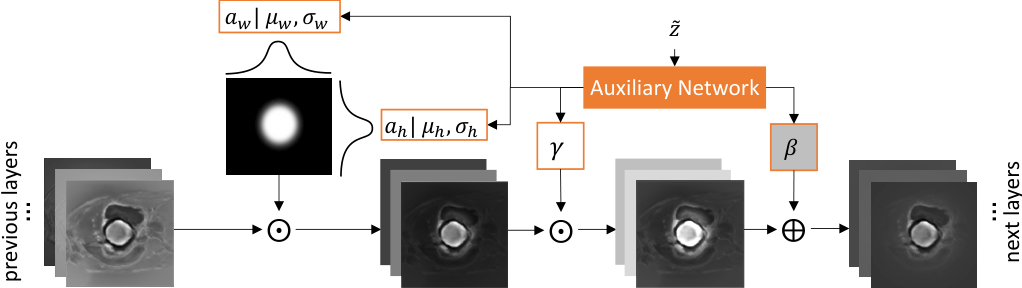
Refer to caption — Figure 1: Visualisation of the method. Given a feature map $F_{c}$ and conditioning vector $\tilde{z}$ , the method first applies spatial attention ( $a$ ) with scale ( $\gamma$ ) and shift ( $\beta$ ) factors to $F_{c}$ respectively. The attention matrix ( $a$ ) is the product of two Gaussian vectors ( $a_{h},a_{w}$ ). Therefore, for a single feature map, the auxiliary network predicts six parameters ( $\gamma$ , $\beta$ , $\mu_{h}$ , $\sigma_{h}$ , $\mu_{w}$ , $\sigma_{w}$ ). We denote Hadamard product with $\odot$ symbol.

Conditioning layers have become the dominant method to tackle this challenge, finding application in image synthesis [3], style transfer [7] and visual question answering (VQA) [16]. In this setup, the network is conditioned on non-imaging information via a learned set of scalar weights which affinely transform feature maps to selectively amplify or suppress each feature, thus controlling its contribution to the final prediction. However, this method has limited capability to adjust channels spatially, and is less suited to conditioning on information relating to spatial or spatio-temporal prior knowledge. Consider a problem where we expect to produce a segmentation only on one side of the image (left or right) indicated by the laterality of the patient’s symptoms. To accomplish this task, the network would require to learn how to encode relative spatial relationships and split them into channels. We show that spatial conditioning can be challenging and propose a method to overcome this limitation.

We present a new conditioning layer which uses non-imaging information to steer spatial attention before applying the affine transformation. We choose a Gaussian for the attention mechanism due to its parameter-efficiency, allowing us to learn a separate attention per channel. However, other differentiable functions can also be used. We first test our method on a simulated dataset, our extension of the CLEVR¹¹ 1 Diagnostic Dataset for Compositional Language and Elementary Visual Reasoning dataset [10], where we segment objects based on their location within the image space. To prove the method is applicable in a clinical setting, we use the ACDC²² 2 Automated Cardiac Diagnosis Challenge (ACDC), MICCAI Challenge 2017 dataset [2] with the task to segment anatomical structures from cardiac cine-MR images. We perform 2D segmentation, and provide slice position and cardiac cycle phase as the non-imaging information to our method.

Contributions: (1) we propose a new conditioning layer capable of handling spatial and spatio-temporal dependency given a conditioning variable; (2) we extend the CLEVR dataset for segmentation tasks and several conditioning scenarios, such as shape-, colour-, or size-based conditioning in the segmentation space; (3) we evaluate different conditioning layers for the task of segmentation on the CLEVR-Seg and ACDC datasets.

2 Related Work

An early work on adapting batch normalisation for conditioning was in style transfer. The conditional instance normalisation layer [6] (Eq. 1) applied a pair of scale ( $\gamma_{s}$ ) and shift ( $\beta_{s}$ ) vectors from the style-dependent parameter matrices, where each pair corresponded to a single style $s$ such as Claude Monet or Edvard Munch. This allowed several styles to be learned using a single network and proved that affine transformations were sufficient for the task. However, the method is restricted to the discrete set of styles seen during training. In Adaptive Instance Normalisation (AdaIN) [7], the authors proposed to instead use a network to predict the style-dependent vectors (as in hypernetworks), allowing parameters to be predicted for arbitrary new styles at inference time.

z=\gamma_{s}\frac{x-\mu_{x}}{\sigma_{x}}+\beta_{s}

(1)

AdaIN has been applied outside of the style transfer domain, for instance to image synthesis using face landmarks where the method is used to inpaint the landmark with face texture [23], and to conditional object segmentation given its coordinates [20]. A similar method to AdaIN was applied to visual question-answering (VQA); the authors used feature-wise linear modulation layer (FiLM) [16] to condition the network with questions. FiLM is identical to AdaIN but omits the instance normalisation step ( $\mu_{x},\sigma_{x}$ in Eq. 1), which the authors found to be unnecessary. FiLM has found application in medical image analysis for disentangled representation learning [4] and for segmentation [9].

A drawback of both AdaIN and FiLM is that they manipulate whole feature maps in an affine fashion, making the methods insensitive to spatial processing. To overcome this limitation, SPADE [15] was proposed, where a segmentation mask is used as a conditioning input in the task of image synthesis, leading to both feature-wise and class-wise scale and shift parameters at each layer. This method is not suitable if the non-imaging information cannot be conveniently expressed in image space.

The closest method to ours is [18]. The authors proposed to extend FiLM with spatial attention, creating a Guiding Block layer, in which the spatial attention is defined as two vectors $\alpha\in\mathbb{R}^{H}$ and $\beta\in\mathbb{R}^{W}$ which are replicated over the $H$ and $W$ axes and added to the global scale factor ( $\gamma_{c}^{(s)}$ ) as shown in Eq. 2 (the authors call the shifting factor as $\gamma_{c}^{(b)}$ ). This spatial conditioning is expensive as there are an additional $H+W$ parameters to learn; perhaps for this reason, a single attention mechanism is learned for each layer and applied across all feature maps.

F^{\prime}_{h,w,c}=(1+\alpha_{h}+\beta_{w}+\gamma_{c}^{(s)})F_{h,w,c}+\gamma_{c}^{(b)}

(2)

In our work, we utilise a learned attention mechanism for each feature map. Our mechanism is similar to [12], where the product of two Gaussian matrices parametrised by mean ( $\mu$ ), standard deviation ( $\sigma$ ) and stride ( $\gamma$ ) between consecutive Gaussians (one Gaussian per row, one matrix per axis) is constructed. However, the relation between standard deviations and strides is estimated before the training and kept fixed. Our method applies a single Gaussian vector per axis (no stride) and we train the whole method end-to-end. Further, the parameters in [12] are estimated using consecutive input images whilst we use an auxiliary conditioning input, and we combine with a FiLM layer.

3 Method

3.1 INstance modulation with SpatIal DEpendency (INSIDE)

Our method adopts the formulation of previous conditioning layers [22] where, given a feature map $F_{c}$ , we apply an affine transformation using scale ( $\gamma$ ) and shift ( $\beta$ ) factors. However, to facilitate spatial manipulation we propose to apply a Gaussian attention mechanism prior to feature-wise linear modulation (FiLM) to process only a (spatially) relevant subset of each feature map. The choice of the attention mechanism, where each matrix is constructed with two Gaussian vectors [( $a_{h}|\mu_{h},\sigma_{h}$ ), ( $a_{w}|\mu_{w},\sigma_{w}$ )] is motivated by parameter efficiency. Therefore, the method can learn one attention mechanism per feature map by adding four additional parameters for each channel (six parameters in total, including the scale and shift factors).

We illustrate the method in Fig. 1. Given a feature map $F_{c}\in\mathbb{R}^{H\times W}$ as input, where $c$ is the channel, we first apply Gaussian attention similar to [12]. We define two vectors $a_{c,h}\in\mathbb{R}^{H}$ and $a_{c,w}\in\mathbb{R}^{W}$ following the Gaussian distribution parametrised by mean and standard deviation to construct an attention matrix $a_{c}=a_{c,h}a_{c,w}^{T}$ . The attention is applied to the feature map prior to feature-wise modulation, i.e.

\text{INSIDE}(F_{c}|\gamma_{c},\beta_{c},a_{c})=F_{c}\odot a_{c}\odot\gamma_{c}+\beta_{c}\text{ .}

(3)

To construct the Gaussian vectors, we normalise the coordinate system, transforming each axis to span the interval $[-1,1]$ . We apply a similar transformation to the standard deviation; the value (the output of a sigmoid activation) lies within the $[0,1]$ range. We set the maximum width to 3.5 standard deviations to cover (at maximum) 99.95% of the image width, thus constraining by design the allowable size of the Gaussian.

3.2 Auxiliary Network

We use a separate auxiliary network (a hypernetwork) for each layer to predict the parameters of INSIDE (see Eq. 3). The network takes a conditional input $\tilde{z}$ to control the Gaussian attention and affine transformation. The information is encoded using a 3-layer MLP arranged as ( $\frac{c}{2}-\frac{c}{2}-6c$ ) where $c$ is the number of channels feeding into the INSIDE layer. We use $tanh$ activation functions except for the last layer where scale ( $\gamma$ ) and shift ( $\beta$ ) factors are predicted with no activation (identity function). The Gaussian’s mean is bounded between $[-1,1]$ (relative position along the axis from the centre), enforced with a $tanh$ function, and we use $sigmoid$ activations to predict the standard deviation of the Gaussian vectors.

3.3 Loss Function

To avoid the network defaulting to a general solution with a large diffuse Gaussian [14], we add an $L_{2}$ regularisation penalty $\eta$ to the cost function to encourage learning of localisation, as in the equation below:

\mathcal{L}=\mathcal{L}_{\text{Dice}}+0.1\cdot\mathcal{L}_{\text{Focal}}+\eta||\sigma||_{2}^{2}\text{ .}

The first part of the cost function relates to the segmentation task and involves a combination of Dice loss [5] (evaluated on the task foreground classes) and Focal loss [13] (evaluated on every class including background). The second part is the penalty applied to our conditioning layer. Throughout the training, we keep $\eta=0.0001$ and the Focal loss focusing parameter $\gamma=0.5$ . The coefficients were selected using a grid search giving reasonable performance across all tested scenarios. We optimise every model with Adam [11] with learning rate set to 0.0001, and $\beta_{1}=0.9$ , $\beta_{2}=0.999$ . We apply early stopping criterion evaluated on validation set using Dice score only.

4 Experiments

We evaluate our method on two datasets and report the Dice coefficient on 3-fold cross validation. Each experiment was further repeated three times using different seeds to avoid variance due to the weight initialisation. We compare our method against the following techniques, as discussed earlier in Section 2:

•

Baseline - a vanilla CNN network without conditioning
•

FiLM [16] - feature-wise affine transformation (also component of INSIDE)
•

Guiding Block [18] - extension of FiLM with spatial attention

4.1 CLEVR-Seg Dataset

We present a novel dataset based on the CLEVR dataset [10], which we name CLEVR-Seg. We have extended the original dataset with segmentation masks and per-object attributes, such as colour (yellow, red, green), location (quadrant containing the centre of mass), shape (cubes, spheres, prisms), and size (small, medium, large). The attributes determine the segmentation task, i.e. segment red objects, segment objects in the bottom left quadrant, etc. The network must thus use the non-imaging information to produce an accurate result. In contrast to the original work, conditioning is provided as categorical one-hot encoded vectors, rather than as natural language questions since VQA is not our primary focus. We generated 4000 random images with 3 to 5 objects each (containing at least one of each shape, size and colour), paired with segmentation masks for which each conditioning factor was drawn at random with equal probability. We split the dataset into training (2880 samples), validation (320), and test (800) subsets which we kept fixed throughout the evaluation. The intensities in each image were normalised to fit the [0, 1] range.

Network:

We use a simple fully-convolutional encoder-decoder with 3 down- and 3 up-sample blocks. Each block consists of ( $3\times 3$ ) kernels followed by ReLU activation function and max-pooling/up-sampling, starting with 16 kernels and doubling/halving at each subsequent step. We test each conditional layer by placing it between the encoder and the decoder, i.e. at the network bottleneck.

Results:

We first evaluate the spatial conditioning scenario. Quantitative results are shown in Table 1 and qualitative examples are presented in Fig. 2 top. We observe that FiLM has poor performance, achieving a Dice score of 0.487 ( $\pm 0.007$ ). This result confirms our hypothesis that spatial conditioning is difficult to disentangle into separate channels, otherwise FiLM would achieve satisfactory performance. On the other hand, the Guiding Block achieves adequate performance with a Dice score of 0.819 ( $\pm 0.033$ ). When we use only one Gaussian attention, INSIDE performs worse than the Guiding Block, however when we use one learned attention per channel, INSIDE performs best, with a Dice score of 0.857 ( $\pm$ 0.025). We further evaluate our attention mechanisms without feature-wise modulation (“Single Attention”, “Multiple Attentions”). These methods yield satisfactory results, although with higher variance. The combination of both gives the highest Dice score and lowest variance across all evaluation scenarios. The use of feature-wise attention mechanisms give more flexibility to learn shape- and size-dependent positional bias. Similar patterns are seen on other conditioning scenarios, i.e. colour, shape and size.

Table 1: Quantitative results on our CLEVR-Seg dataset where we condition on a quadrant (spatial conditioning), object colour, shape and size. We report Dice scores (multiplied by 100) with standard deviations shown as subscripts. The method with highest average result is presented in bold. We use the Wilcoxon test to assess statistical significance between INSIDE (with multiple attentions) and the best baseline method. We denote two (**) asterisks for

p\leqslant 0.01

Method Quadrant Colour Shape Size Baseline $29.3_{0.7}$ $28.5_{0.2}$ $27.6_{0.2}$ $27.3_{1.2}$ FiLM $48.7_{2}$ $89.8_{2}$ $87.7_{1.2}$ $84.2_{2}$ Guiding Block $81.9_{3.3}$ $89.3_{5}$ $89.9_{2}$ $84.3_{3}$ Single Attention (w/o FiLM) $50.2_{0.7}$ $81.5_{7.5}$ $79.2_{6.9}$ $80.8_{2.5}$ Multiple Attentions (w/o FiLM) $82.4_{3.8}$ $90.1_{2.9}$ $88.3_{5.9}$ $\textbf{85.4}_{2.1}$ INSIDE (Single Attention) $77.9_{2.5}$ $87.8_{0.6}$ $89.8_{0.7}$ $\textbf{85.4}_{0.8}$ INSIDE (Multiple Attentions) $\textbf{85.7}^{**}_{2.5}$ $\textbf{90.7}^{**}_{1.9}$ $\textbf{90.7}^{**}_{1.9}$ $\textbf{85.4}^{**}_{1.2}$

4.2 ACDC Dataset

The ACDC dataset [2] contains cine-MR images of 3 cardiac structures, the myocardium and the left and right ventricular cavities, with the task to segment these anatomies. The annotated dataset contains images at end-systolic and -diastolic phases from 100 patients, at varying spatial resolutions. We resample the volumes to the common resolution of 1.37 mm² per pixel, resize each slice to $224\times 224$ pixels, clip outlier intensities within each volume outside the range $[5\%,95\%]$ , and finally standardise the data to be within the [0, 1] range.

Conditioning.

We evaluate two conditioning scenarios: slice position and phase. Slice position is normalised between $[0,1]$ (from apical slice to basal slice), and cardiac cycle phase, i.e. end-systolic or -diastolic, is encoded as a one-hot vector.

Network.

To segment the images, we train a U-Net [17] network with 4-down and 4-up sampling blocks, Batch Normalisation [8] and ReLU activations, with a softmax for final classification. The architecture selection was motivated by its state-of-the-art results on the ACDC dataset [2]. The conditional layers are placed along the decoding path between consecutive convolutional blocks (each stage has two convolutional blocks). The diagrams can be found in the supplemental material.

Table 2: Quantitative results on ACDC dataset where each image is provided with slice position within the heart volume or phase (end-systolic or end-diastolic). We report average Dice score (multipled by 100) across all anatomical structures evaluated on whole volumes. The method with highest Dice score is presented in bold. We use the Wilcoxon test to assess statistical significance between INSIDE and the second best method. We denote one (*) and two (**) asterisks for

p\leqslant 0.1

and

p\leqslant 0.01

respectively. We apply Bonferroni correction (

m=2

) to account for multiple comparisons (when comparing to “Baseline”).

Method 100% dataset 25% dataset 6% dataset Position Phase Position Phase Position Phase Baseline $87_{1.9}$ $78.2_{2.5}$ $53.6_{6}$ FiLM $84.7_{4.5}$ $85.4_{3.9}$ $73.4_{16.3}$ $76_{5.4}$ $59.9_{5.4}$ $55.7_{7.6}$ Guiding Block $83.7_{4}$ $76.2_{21.4}$ $77.8_{2}$ $77.6_{2.4}$ $53.7_{5.5}$ $54.8_{5}$ INSIDE $\textbf{87.8}^{**}_{1.5}$ $\textbf{87.7}^{*}_{1.6}$ $\textbf{80.2}^{**}_{1.4}$ $\textbf{78.9}^{*}_{1.8}$ $\textbf{62.2}^{*}_{5.2}$ $\textbf{61.4}^{**}_{3.8}$

Results.

The empirical results on the ACDC dataset are presented in Table 2, with varying fractions of the training set, i.e. at 100%, 25%, and 6%. Overall, our method achieves consistent improvement over the baseline (when no conditioning information is provided) with better relative performance as the size of the training dataset decreases (+0.9%, +2.6%, +16% Dice respectively). We argue the networks rely more on non-imaging information when the number of training examples is reduced. We further present selected segmentation results and visualise how the attention changes depending on the conditioning information (Fig. 3). Across the evaluation scenarios, we notice conditioning on slice position generally yields the highest improvement, which is expected as there is a clear link between position and heart size (expressed by the Gaussian’s standard deviation). The proposed method achieved the highest average Dice score across all tested scenarios. The Guiding Block underperforms in most experiments, and we argue that our choice of Gaussian attention imposes a beneficial shape prior for the heart. FiLM performs well (at 6% training data) when position is provided as the conditioning information, but underperforms comparing to our method; this is logical since non-imaging information helps to inform the network about the expected size of segmentation masks, but does not have enough flexibility to spatially manipulate features maps as our method.

5 Conclusion

Endowing convolutional architectures with the ability to peruse non-imaging information is an important problem for our community but still remains challenging. In this work, we have proposed a new conditional layer which extends FiLM with Gaussian attention that learns spatial dependencies between image inputs and non-imaging information when provided as condition. We have shown the attention mechanism allows spatial-dependency to be modelled in conditional layers. Our method is low in parameters, allowing efficient learning of feature-wise attention mechanisms which can be applied to 3D problems by adding an additional orthogonal 1D Gaussian for each channel.

Acknowledgments

This work was supported by the Engineering and Physical Sciences Research Council [grant number EP/R513209/1]; and Canon Medical Research Europe Ltd. S.A. Tsaftaris acknowledges the support of the Royal Academy of Engineering and the Research Chairs and Senior Research Fellowships scheme.

References

[1] Bai, W., Sinclair, M., Tarroni, G., Oktay, O., Rajchl, M., Vaillant, G., Lee, A.M., Aung, N., Lukaschuk, E., Sanghvi, M.M., et al.: Automated cardiovascular magnetic resonance image analysis with fully convolutional networks. Journal of Cardiovascular Magnetic Resonance 20(1), 65 (2018)
[2] Bernard, O., Lalande, A., Zotti, C., Cervenansky, F., Yang, X., Heng, P.A., Cetin, I., Lekadir, K., Camara, O., Ballester, M.A.G., et al.: Deep Learning Techniques for Automatic MRI Cardiac Multi-Structures Segmentation and Diagnosis: Is the Problem Solved? IEEE Transactions on Medical Imaging 37(11), 2514–2525 (2018)
[3] Brock, A., Donahue, J., Simonyan, K.: Large Scale GAN Training for High Fidelity Natural Image Synthesis. arXiv preprint arXiv:1809.11096 (2018)
[4] Chartsias, A., Joyce, T., Papanastasiou, G., Semple, S., Williams, M., Newby, D.E., Dharmakumar, R., Tsaftaris, S.A.: Disentangled representation learning in cardiac image analysis. Medical Image Analysis 58, 101535 (2019)
[5] Dice, L.R.: Measures of the Amount of Ecologic Association Between Species. Ecology 26(3), 297–302 (1945)
[6] Dumoulin, V., Shlens, J., Kudlur, M.: A Learned Representation For Artistic Style. arXiv preprint arXiv:1610.07629 (2016)
[7] Huang, X., Belongie, S.: Arbitrary Style Transfer in Real-time with Adaptive Instance Normalization. In: Proceedings of the IEEE International Conference on Computer Vision. pp. 1501–1510 (2017)
[8] Ioffe, S., Szegedy, C.: Batch Normalization: Accelerating Deep Network Training by Reducing Internal Covariate Shift. arXiv preprint arXiv:1502.03167 (2015)
[9] Jacenków, G., Chartsias, A., Mohr, B., Tsaftaris, S.A.: Conditioning Convolutional Segmentation Architectures with Non-Imaging Data. In: International Conference on Medical Imaging with Deep Learning–Extended Abstract Track (2019)
[10] Johnson, J., Hariharan, B., van der Maaten, L., Fei-Fei, L., Lawrence Zitnick, C., Girshick, R.: CLEVR: A Diagnostic Dataset for Compositional Language and Elementary Visual Reasoning. In: Proceedings of the IEEE Conference on Computer Vision and Pattern Recognition. pp. 2901–2910 (2017)
[11] Kingma, D.P., Ba, J.: Adam: A Method for Stochastic Optimization. arXiv preprint arXiv:1412.6980 (2014)
[12] Kosiorek, A., Bewley, A., Posner, I.: Hierarchical Attentive Recurrent Tracking. In: Advances in Neural Information Processing Systems. pp. 3053–3061 (2017)
[13] Lin, T.Y., Goyal, P., Girshick, R., He, K., Dollár, P.: Focal Loss for Dense Object Detection. In: Proceedings of the IEEE International Conference on Computer Vision. pp. 2980–2988 (2017)
[14] Nibali, A., He, Z., Morgan, S., Prendergast, L.: Numerical Coordinate Regression with Convolutional Neural Networks. arXiv preprint arXiv:1801.07372 (2018)
[15] Park, T., Liu, M.Y., Wang, T.C., Zhu, J.Y.: Semantic Image Synthesis with Spatially-Adaptive Normalization. In: Proceedings of the IEEE Conference on Computer Vision and Pattern Recognition. pp. 2337–2346 (2019)
[16] Perez, E., Strub, F., De Vries, H., Dumoulin, V., Courville, A.: FiLM: Visual Reasoning with a General Conditioning Layer. In: Thirty-Second AAAI Conference on Artificial Intelligence (2018)
[17] Ronneberger, O., Fischer, P., Brox, T.: U-Net: Convolutional Networks for Biomedical Image Segmentation. In: International Conference on Medical Image Computing and Computer-Assisted Intervention. pp. 234–241. Springer (2015)
[18] Rupprecht, C., Laina, I., Navab, N., Hager, G.D., Tombari, F.: Guide Me: Interacting with Deep Networks. In: Proceedings of the IEEE Conference on Computer Vision and Pattern Recognition. pp. 8551–8561 (2018)
[19] Sato, S., Koga, M., Yamagami, H., Okuda, S., Okada, Y., Kimura, K., Shiokawa, Y., Nakagawara, J., Furui, E., Hasegawa, Y., et al.: Conjugate eye deviation in acute intracerebral hemorrhage: stroke acute management with urgent risk-factor assessment and improvement–ich (samurai-ich) study. Stroke 43(11), 2898–2903 (2012)
[20] Sofiiuk, K., Barinova, O., Konushin, A.: AdaptIS: Adaptive Instance Selection Network. In: Proceedings of the IEEE International Conference on Computer Vision. pp. 7355–7363 (2019)
[21] Stoyanov, D., Taylor, Z., Ferrante, E., Dalca, A.V., Martel, A., Maier-Hein, L., Parisot, S., Sotiras, A., Papiez, B., Sabuncu, M.R., et al.: Graphs in Biomedical Image Analysis and Integrating Medical Imaging and Non-Imaging Modalities: Second International Workshop, GRAIL 2018 and First International Workshop, Beyond MIC 2018, Held in Conjunction with MICCAI 2018, Granada, Spain, September 20, 2018, Proceedings, vol. 11044. Springer (2018)
[22] Ulyanov, D., Vedaldi, A., Lempitsky, V.: Instance Normalization: The Missing Ingredient for Fast Stylization. arXiv preprint arXiv:1607.08022 (2016)
[23] Zakharov, E., Shysheya, A., Burkov, E., Lempitsky, V.: Few-Shot Adversarial Learning of Realistic Neural Talking Head Models. arXiv preprint arXiv:1905.08233 (2019)