Spatial clustering of depinning avalanches in presence of long-range interactions
Abstract
Disordered elastic interfaces display avalanche dynamics at the depinning transition. For short-range interactions, avalanches correspond to compact reorganizations of the interface well described by the depinning theory. For long-range elasticity, an avalanche is a collection of spatially disconnected clusters. In this paper we determine the scaling properties of the clusters and relate them to the roughness exponent of the interface. The key observation of our analysis is the identification of a Bienaymé-Galton-Watson process describing the statistics of the cluster number. Our work has a concrete importance for experimental applications where the cluster statistics is a key probe of avalanche dynamics.
Many catastrophic phenomena such as epidemic outbreaks, earthquakes Fisher et al. 1997; Jagla et al. 2014; de Arcangelis et al. 2016 or financial crashes are initiated by a single unstable (or infected) seed that destabilizes many other elements. The instability propagates as a cascade where each unstable element triggers a number of offsprings. These processes are also observed in the response of disordered systems to small perturbations and are called avalanches Sethna et al. 2001. The cascades of plastic events in amorphous materials Lin et al. 2014; Baret et al. 2002, the ground-state reorganizations of mean-field spin glasses Le Doussal et al. 2012; Franz and Spigler 2017 or the jerky motion of fronts propagating in heterogeneous media Fisher 1998; Kardar 1998 are examples of such avalanches.
We can consider that the first model of avalanches was introduced by Bienaymé Bienaymé 1845 and by Galton and Watson Watson and Galton 1875 who were interested in the extinction probability of surnames. In this model the number of offsprings per individual is an independent identically distributed random variable whose average determines the fate of the process. If there is a finite probability that the surname never gets extinct, while for the surname gets extinct with probability one. In this case the family size (total number of descendants of an individual) is a stochastic variable displaying a power law distribution , with exponent , which is truncated (exponentially) above a maximal size .

We are interested in the avalanches observed when elastic interfaces of dimension , such as magnetic domain walls Zapperi et al. 1998; Laurson et al. 2013; Durin et al. 2016, crack fronts Gao and Rice 1989; Tanguy et al. 1998; Bonamy et al. 2008; Bonamy and Bouchaud 2011; Ponson 2016 or wetting lines Joanny and de Gennes 1984; Roux et al. 2003; Moulinet et al. 2004; Le Doussal et al. 2009a, propagate in heterogeneous materials. Under the action of an external force , the front remains pinned up to a critical force where it undergoes a depinning transition. At the depinning point the front is in a random self-affine configuration characterized by the roughness exponent , whose value is known from numerical simulations Rosso and Krauth 2002; Rosso et al. 2003 and Functional Renormalization Group calculations Nattermann et al. 1992; Narayan and Fisher 1993; Ertaş and Kardar 1994; Le Doussal et al. 2002. Near depinning, small perturbations can trigger avalanches which are large rearrangements of the front, of total size . In presence of short-range (SR) elasticity, avalanches are spatially connected and the size exponent is smaller than the one predicted by the Bienaymé-Galton-Watson (BGW) model. Indeed spatial information is absent from the BGW model while one expects that, for an unstable point of the interface, the analog of the number of offsprings depends on its generation and its position. At variance with BGW, the avalanche of an interface has a spatial location characterized by a linear size that displays a power law distribution . In the framework of the depinning theory we know that and that the avalanche exponents are not independent but related to the roughness exponent via the relations and Narayan and Fisher 1993.
In many physical situations, fronts are however characterized by a long-range (LR) elastic kernel that decays as . In particular it has been shown that the elasticity of crack fronts Rice 1985; Gao and Rice 1989 and wetting lines Joanny and de Gennes 1984 is LR with . The shape of the interface is affected by the range of the interactions. As a function of we idenfity three regimes : (i) the mean-field (MF) case, for , where the interface is flat and , (ii) for the interface is rough and grows with , (iii) for , saturates to its SR value. LR interactions also affect the avalanche statistics, the depinning theory extends to the scaling relation for the size distribution. In particular in the MF case we recover the BGW value , while for we have Narayan and Fisher 1993; Zapperi et al. 1998; Dobrinevski et al. 2014 :
| (1) | ||||
| (2) |
The second equation derives from the first one via the self-affinity relation . Beyond this modification, LR avalanches are qualitatively different from SR ones as they are in general disconnected objects. An example of an avalanche for is shown in Fig. 1. It is composed of disconnected clusters. We denote the (random) size of a given cluster, and its extension. A gap between two clusters is denoted by . We define the linear size of the avalanche as the sum of the extensions of its clusters, noted schematically . This length is much shorter than the diameter of the region affected by the reorganization.
All these quantities display power law statistics with exponents that we aim to determine. This is particularly important for experiments where the spatial structure is accessible Måløy et al. 2006; Tallakstad et al. 2011. In these experiments the perturbation is provided by a continuous drive and independently triggered avalanches can overlap in time and/or space Barés et al. 2013; Janićević et al. 2016; Le Priol et al. 2020. This makes the reconstruction of LR avalanches difficult and clusters, which are simple to identify, remain the reliable probe of the universal properties of avalanche dynamics.
The first attempt to characterize the cluster statistics of LR depinning avalanches was done in Ref. Laurson et al. 2010, where, based on numerical simulations for , a scaling relation for the cluster size exponent was proposed and justified by arguments that we show to be incorrect. This relation was experimentally confirmed in Tallakstad et al. 2011 for . In this Letter we derive scaling relations for all cluster exponents, and for all and show that they depend only on the roughness exponent (see table 1 for a summary of the results). The validity of our relations is based on the key numerical observation, unveiled here, that the distribution of appears to obey the BGW statistics : each cluster triggers a number of offsprings which can be considered as an independent and identically distributed random variable.

Let us start by defining the cellular automaton model, already used in Schmittbuhl et al. 1995; Laurson et al. 2010; Le Priol et al. 2020, for the simulations of depinning interfaces. Consider a one-dimensional interface (i.e. a line) where is the time, the internal coordinate and the displacement field (see Fig. 1). We assume that all time and space variables and are integers, that the line size is and we implement periodic boundary conditions . The disorder pins the line up to a local threshold force balanced by the force
| (3) |
where the first term describes the driving force deriving from a harmonic confinement of curvature and the second is the LR elastic force. The local thresholds are independent identically distributed numbers drawn from the positive part of a normal distribution. The harmonic confinement induces a characteristic transversal length beyond which the interface is flattened. At time if the point is stable while if the point is unstable : it topples, namely , and the new threshold is drawn. Avalanches are produced in a quasi-static protocol : when all points are stable is increased up to a value at which a first instability occurs and the dynamics unfolds until the line reach a new stable configuration. We focus on the stationary regime of avalanches, reached after a transient when starting from an arbitrary configuration. Our simulations are performed for a line of size for , 0.75, 1 and 1.5 and many values of the curvature for each . The details of the parameters are given in the Supplemental Material (Sup). Note that the positive curvature sets the distance from the critical point (at ) and controls the cutoffs of all power law distributions. It corresponds to in the BGW model.
This model was implemented in Ref. Laurson et al. 2010 for and the analysis of the data led to conjecture the following scaling relation for the cluster size exponent :
| (4) |
The justification of this relation was based on two assumptions : (i) During the avalanche spreading the evolution of the number of clusters is interpreted as a discrete random walk with the time replaced by the number of topplings. At each time step, the number of clusters can increase by , remain constant, or decrease by . This implies that the average number of clusters at the end of avalanches of size (equal to the total number of topplings) scales as . The assumption that the process is Markovian leads to . (ii) The clusters belonging to an avalanche of size have a typical size and applying one finds foo :
| (5) |
which yields (4) for . In the case , the value of was found numerically to be compatible with . In figure 2 we extend the study to . We find that in general and that it decreases continuously with . Inserting our measured values of in (5) yields predictions for that differ from the observed values (e.g. for we measured and while (5) yields ). Equation (5) is wrong as the assumption (ii) is incorrect : clusters belonging to avalanches of size do not have the same typical size but are broadly distributed according to a power law distribution for up to . This implies and thus instead of (5) (see Sup). The exponent , which varies continuously with , is not independent but is related to as we demonstrate by studying the distribution of the cluster number .
In figure 3 we study the statistics of the cluster number for different values of and . In order to produce a collapse for different values of we adopt the procedure described in Rosso et al. 2009 : we introduce the variable and compute the function defined as :
| (6) |

For small values of the curvature, is fully universal and its analytical form is known for the BGW process and reads Le Doussal et al. 2009b; Le Doussal and Wiese 2009 :
| (7) |
Remarkably the data seem to collapse on the same universal curve for all and cannot be clearly distinguished from the BGW function of equation (7). In the case one expects that the number of clusters is proportional to the avalanche size (up to logarithmic corrections). Thus it is not too surprising to recover a BGW shape in this case, since, in mean-field, this is the distribution of the avalanche size. It is however much less clear why this behavior should hold for . Numerically we cannot exclude that is BGW (in the limit , ) also for , and . However, for what follows we need only to assume that and we do not mind about the exact decay at large scale. To conclude the argument it is sufficient to remark that (see Sup where we show that is peaked around ) which yields . Combined with the relation obtained above, we arrive at the scaling relation (4) which we thus find to be valid for all , by a completely different mechanism from Laurson et al. 2010. Note that we can also infer that the cutoff of scales as .
The same reasoning can be repeated to find the relation between the extension of an avalanche and the extension of the clusters. Using the definition for , , we first derive the relation . Then assuming that the distribution of originates from a BGW process we derive :
| (8) |
by using . Note that from , and we can also derive which corresponds to the self-affine property of the clusters (see Sup).

The scaling relations that we have derived allow to express all the exponents as functions of and . We have collected all these expressions in table 1 and compared the predicted values of the exponents with the ones directly measured in our numerical simulations. We found good agreements for all values of .
Note that at variance with SR elasticity the diameter of the region that is perturbed by the presence of an avalanche does not coincide with the avalanche linear size . The diameter is in general much larger than and displays novel statistical properties that we should characterize.
In figure 4 we show the diameter distribution for , 1 and 1.5. For a crossover separates two power law decays :
Remarkably the exponent is independent with a numerical value close to (also for ). Hence the statistics of the diameter is very different from the one of the linear size . Since , where is the total gap, we need to investigate the statistics of the gaps . Their distributions, shown in the inset of figure 4, present a crossover between two power law decays :
with independently from . Since the decay of is much slower than the one of (which decays faster than any power law at large scale, see Sup), we expect which implies that . This latter relation is confirmed by figure 4 where the distribution of and are plotted together and are indistinguishable.
The scaling form (Spatial clustering of depinning avalanches in presence of long-range interactions) can now be derived from the gap distribution (Spatial clustering of depinning avalanches in presence of long-range interactions). Let us first consider avalanches where all gaps are below . In this case we can write :
| (13) |
where we used since for up to (see Sup). Again using and setting we find :
| (14) |
which is close from the exponent we measure . A very large value of corresponds to the presence of one (or a very few) gap . This gap has a probability and dominates which hence also has a probability .
The main result of this paper is to show that, even in presence of LR interactions, the statistical properties of depinning avalanches can always be expressed as functions of the elasticity range parameter and the roughness exponent . Our conclusions are based on the numerical observation that the number of clusters behave as the number of offsprings of a BGW model for all between and . We are not able to demonstrate this conjecture but our numerics shows that it is a very good approximation. All relations between the exponents of clusters and global avalanches are based on this conjecture so it would be of great interest to show it analytically. It would be also interesting to characterize the statistical properties of the clusters of plastic avalanches Baret et al. 2002; Lin et al. 2014; Salerno et al. 2012; Nicolas et al. 2018. Indeed the Eshelby kernel, which is the relevant interaction for the yielding transition, is long-range (with ) but, in contrast with depinning, non-monotonous.
Acknowledgements.
Acknowledgments: We thank L. Ponson for enlightening discussions. PLD acknowledges support from ANR under the grant ANR- 17-CE30-0027-01 RaMaTraF| measured / prediction | ||||||
|---|---|---|---|---|---|---|
| Exponent | Expression | Relation | ||||
| 0 (MF) | 0.18(1) | 0.39 Rosso and Krauth 2002 | 0.75(2) | |||
| 0.89(2) / 1 | 0.73(1) / 0.73(1) | 0.52(2) / 0.56 | 0.29(1) / 0.28(2) | |||
| 0.93(2) / 1 ; | 0.80(2) / 0.86(2) | 0.70(2) / 0.78 | 0.50(2) / 0.54(4) | |||
| 1.50(1) / | 1.36(2) / 1.36(1) | 1.26(2) / 1.28 | 1.14(2) / 1.14(1) | |||
| 2.00(9) / 2 | 1.72(4) / 1.73(1) | 1.56(2) / 1.56 | 1.28(2) / 1.28(2) | |||
| 1.50(2) / | 1.38(5) / 1.43(1) | 1.33(5) / 1.39 | 1.20(3) / 1.25(2) | |||
| 2.05(5) / 2 | 1.90(5) / 1.86(2) | 1.80(2) / 1.78 | 1.45(3) / 1.50(4) | |||
References
- Fisher et al. (1997) D. S. Fisher, K. Dahmen, S. Ramanathan, and Y. Ben-Zion, Phys. Rev. Lett. 78, 4885 (1997).
- Jagla et al. (2014) E. A. Jagla, F. P. Landes, and A. Rosso, Phys. Rev. Lett. 112, 174301 (2014).
- de Arcangelis et al. (2016) L. de Arcangelis, C. Godano, J. R. Grasso, and E. Lippiello, Physics Reports 628, 1 (2016).
- Sethna et al. (2001) J. P. Sethna, K. A. Dahmen, and C. R. Myers, Nature 410, 242 (2001).
- Lin et al. (2014) J. Lin, E. Lerner, A. Rosso, and M. Wyart, Proc. Natl. Acad. Sci. 111, 14382 (2014).
- Baret et al. (2002) J.-C. Baret, D. Vandembroucq, and S. Roux, Phys. Rev. Lett. 89, 195506 (2002).
- Le Doussal et al. (2012) P. Le Doussal, M. Müller, and K. J. Wiese, Phys. Rev. B 85, 214402 (2012).
- Franz and Spigler (2017) S. Franz and S. Spigler, Phys. Rev. E 95, 022139 (2017).
- Fisher (1998) D. S. Fisher, Phys. Rep. 301, 113 (1998).
- Kardar (1998) M. Kardar, Physics Reports 301, 85 (1998).
- Bienaymé (1845) I.-J. Bienaymé, Soc. Philomat. Paris Extraits, Sér 5, 4 (1845).
- Watson and Galton (1875) H. W. Watson and F. Galton, The Journal of the Anthropological Institute of Great Britain and Ireland 4, 138 (1875).
- Zapperi et al. (1998) S. Zapperi, P. Cizeau, G. Durin, and H. E. Stanley, Phys. Rev. B 58, 6353 (1998).
- Laurson et al. (2013) L. Laurson, X. Illa, S. Santucci, K. Tore Tallakstad, K. J. Måløy, and M. J. Alava, Nat. Commun. 4, 2927 (2013).
- Durin et al. (2016) G. Durin, F. Bohn, M. A. Corrêa, R. L. Sommer, P. Le Doussal, and K. J. Wiese, Phys. Rev. Lett. 117, 087201 (2016).
- Gao and Rice (1989) H. Gao and J. Rice, J. Appl. Mech.-Trans. Asme - J APPL MECH 56, 828 (1989).
- Tanguy et al. (1998) A. Tanguy, M. Gounelle, and S. Roux, Phys. Rev. E 58, 1577 (1998).
- Bonamy et al. (2008) D. Bonamy, S. Santucci, and L. Ponson, Phys. Rev. Lett. 101, 045501 (2008).
- Bonamy and Bouchaud (2011) D. Bonamy and E. Bouchaud, Physics Reports 498, 1 (2011).
- Ponson (2016) L. Ponson, Int J Fract 201, 11 (2016).
- Joanny and de Gennes (1984) J. F. Joanny and P. G. de Gennes, The Journal of Chemical Physics 81, 552 (1984).
- Roux et al. (2003) S. Roux, D. Vandembroucq, and F. Hild, European Journal of Mechanics - A/Solids 22, 743 (2003).
- Moulinet et al. (2004) S. Moulinet, A. Rosso, W. Krauth, and E. Rolley, Phys. Rev. E 69, 035103 (2004).
- Le Doussal et al. (2009a) P. Le Doussal, K. Wiese, S. Moulinet, and E. Rolley, EPL Europhys. Lett. 87, 56001 (2009a).
- Rosso and Krauth (2002) A. Rosso and W. Krauth, Phys. Rev. E 65, 025101 (2002).
- Rosso et al. (2003) A. Rosso, A. K. Hartmann, and W. Krauth, Phys. Rev. E 67, 021602 (2003).
- Nattermann et al. (1992) T. Nattermann, S. Stepanow, L.-H. Tang, and H. Leschhorn, J. Phys. II France 2, 1483 (1992).
- Narayan and Fisher (1993) O. Narayan and D. S. Fisher, Phys. Rev. B 48, 7030 (1993).
- Ertaş and Kardar (1994) D. Ertaş and M. Kardar, Phys. Rev. E 49, R2532 (1994).
- Le Doussal et al. (2002) P. Le Doussal, K. J. Wiese, and P. Chauve, Phys. Rev. B 66, 174201 (2002).
- Rice (1985) J. R. Rice, J. Appl. Mech 52, 571 (1985).
- Dobrinevski et al. (2014) A. Dobrinevski, P. L. Doussal, and K. J. Wiese, EPL Europhys. Lett. 108, 66002 (2014).
- Måløy et al. (2006) K. J. Måløy, S. Santucci, J. Schmittbuhl, and R. Toussaint, Phys. Rev. Lett. 96, 045501 (2006).
- Tallakstad et al. (2011) K. T. Tallakstad, R. Toussaint, S. Santucci, J. Schmittbuhl, and K. J. Måløy, Phys. Rev. E 83, 046108 (2011).
- Barés et al. (2013) J. Barés, L. Barbier, and D. Bonamy, Phys. Rev. Lett. 111, 054301 (2013).
- Janićević et al. (2016) S. Janićević, L. Laurson, K. J. Måløy, S. Santucci, and M. J. Alava, Phys. Rev. Lett. 117, 230601 (2016).
- Le Priol et al. (2020) C. Le Priol, J. Chopin, P. Le Doussal, L. Ponson, and A. Rosso, Phys. Rev. Lett. 124, 065501 (2020).
- Laurson et al. (2010) L. Laurson, S. Santucci, and S. Zapperi, Phys. Rev. E 81, 046116 (2010).
- Schmittbuhl et al. (1995) J. Schmittbuhl, S. Roux, J.-P. Vilotte, and K. Jorgen Måløy, Phys. Rev. Lett. 74, 1787 (1995).
- (40) See Supplemental Material.
- (41) For convenience, here and below we use the same letter to denote the probability densities of all observables.
- Rosso et al. (2009) A. Rosso, P. L. Doussal, and K. J. Wiese, Phys. Rev. B 80, 144204 (2009).
- Le Doussal et al. (2009b) P. Le Doussal, A. Alan Middleton, and K. Wiese, Phys. Rev. E Stat. Nonlin. Soft Matter Phys. 79, 050101 (2009b).
- Le Doussal and Wiese (2009) P. Le Doussal and K. J. Wiese, Phys. Rev. E 79, 051106 (2009).
- Salerno et al. (2012) K. M. Salerno, C. E. Maloney, and M. O. Robbins, Phys. Rev. Lett. 109, 105703 (2012).
- Nicolas et al. (2018) A. Nicolas, E. E. Ferrero, K. Martens, and J.-L. Barrat, Rev. Mod. Phys. 90, 045006 (2018).
Supplemental Material for Spatial clustering of depinning avalanches in presence of long-range interactions
In this supplemental material we give the details of the analysis of our extensive numerical simulations. In appendix A we give the details of the parameters used for the simulations. In appendix B we detail the measurement of the exponents describing the avalanche statistics. Finally, in appendix C we verify the assumptions made in our argument in the main text.
.1 A) Details of the parameters
Figure 5 summarizes the values of the parameters used in the simulations as well as the color code used in all figures except figure 4 of the main text and figure 10 of the supplemental material.
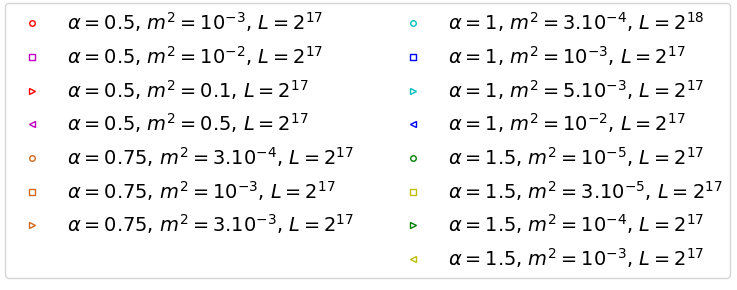
The parameters used in figure 4 of the main text are given below while the ones used in figure 10 of the Supplemental Material are specified in the caption.
Main panel of figure 4 :
: and (red symbols) and and (magenta) ; : and (blue) and and (cyan) ; : and (yellow) and and (green).
Inset of figure 4 :
: and (magenta triangles) and and (red squares) ; : and (cyan circles), and (blue triangles) and and (cyan squares) ; : and (yellow squares) and and (green triangles).
.2 B) Measurement of the exponents

In this section we present the analysis of our extensive numerical simulations in order to measure directly the exponents of the avalanche statistics. All the measurements with error margins are summarized in table 3.
Roughness exponent
The roughness exponent is determined from the recorded stable configurations , using the structure factor :
| (15) | ||||
| (16) |
with the internal dimension of the interface. The overline denotes average over disorder. In practice the average is performed over many stable configurations visited by the line during the simulation. Equation (15) is valid for . Slopes smaller than correspond to with logarithmic corrections. We compute for each , using the smallest values of the curvature used in the simulations. The results are plotted in figure 6.
Our best fit values of are given in table 2 where they are compared with the one loop and two loop calculations from the Functional RG, which are (presumably divergent) series expansions in to order and respectively. Setting simply in these series the one loop result is Ertaş and Kardar 1994; Le Doussal et al. 2002. The two loop result reads , from formula (4.17) and (3.60) in Ref. Le Doussal et al. 2002 (we noted that the integral in (3.60) can be performed explicitly). Note that these formula can also be seen as an expansion around for fixed . For there exists a previous more precise numerical determination Rosso and Krauth 2002. It is this value that we used for computing the numerical values of the predictions in the table of the main text.
| from Fig. 6 | ||||
|---|---|---|---|---|
| 0 | ||||
| 0 | 0.21 | 0.46 | 0.96 |
Avalanche exponents
We now focus on the exponents of the global avalanche. We expect the avalanche size and linear size to obey the following distributions :
| (17) | ||||
| (18) |
where and are some scaling functions that are constant for and present a fast decay for . The cutoff scales and are controlled by the harmonic confinement curvature . It induces a characteristic length beyond which the line is flattened. This length is a natural cutoff for the avalanche linear size distribution. Thanks to the self-affinity property of the avalanches it also sets the cutoff for the total avalanche size .
The avalanche global and linear size distributions are plotted in figure 7. The dashed lines correspond to fits of the exponent and listed in table 3. The data have been rescaled using the cutoff scales and . The collapse of the data for each is a confirmation of the scaling of the cutoffs as well as of the values of the exponents.


Definition of the cluster distribution
In this paper we define the distribution of cluster size as follows. We take avalanches, which have different cluster number , and let be the th cluster of avalanche . Then taking the limit we define :
| (19) |
This prescription amounts to pick one cluster at random among all clusters of all avalanches. The definition of the conditional probability is the same where one selects only avalanches of size . From our definition we can derive the equality used in the main text. Indeed considering avalanches of equal size the average of the cluster sizes over these avalanches is :
| (20) |
Cluster exponents
We expect the cluster size and cluster extension to obey the following distributions :
| (23) | ||||
| (24) |
with scaling functions and that are constant for and decay fast for . Note that we use the same cutoff scales and as for the global avalanches.
The cluster size and extension distributions are plotted in figure 8. The dashed lines correspond to fits of the exponent and listed in table 3. The data have been rescaled using the cutoff scales and . The collapse of the data for each is a confirmation of the scaling of the cutoffs as well as of the values of the exponents.


| Exponent | Expression | ||||
|---|---|---|---|---|---|
| 0.89(1) | 0.73(1) | 0.52(1) | 0.29(1) | ||
| 0.93(2) | 0.80(2) | 0.70(2) | 0.50(2) | ||
| 1.50(1) | 1.36(2) | 1.26(2) | 1.14(2) | ||
| 2.00(10) | 1.72(4) | 1.56(2) | 1.28(2) | ||
| 1.50(2) | 1.38(5) | 1.33(4) | 1.20(3) | ||
| 2.05(5) | 1.90(5) | 1.80(2) | 1.45(3) | ||
| 1.20(7) | 1.15(5) | 1.20(10) | 1.21(6) | ||
| 1.50(2) | 1.50(3) | 1.50(6) | 1.50(8) | ||
| 1.50(5) | 1.50(3) | 1.50(5) | 1.50(6) |
.3 C) Verification of the assumptions


In this section we verify the assumptions made in the argument of the main text.
Self-affinity relations
A basic ingredient of the depinning theory is the self-affinity of the interface. As a consequence the avalanches display the scaling
| (25) |
which is well-verified for short-range avalanches. In figure 9 we test that this scaling also holds for long-range avalanches, both for the global avalanches and the clusters, . The latter relation is also a consequence of the scaling analysis presented in the main text and yields a scaling relation for the cluster exponents :
| (26) |


Relation between and
An important assumption of the derivation proposed in Ref. Laurson et al. 2010 is that the cluster size scales as . This means that for a given avalanche the clusters have similar sizes. As a consequence one could set which yields . We argued that the latter relation is wrong because the clusters in a given avalanche display very different sizes, from very small up to the avalanche size. In figure 10 we show the distribution of cluster sizes conditioned by the total size of the avalanche they belong to. displays a power law for up to that we fit with the same exponent as the unconditioned distribution . Note that the normalization constant does not depend on (as one can see in figure 10) but only on a small scale cutoff . Indeed we have :
Therefore the scaling for the mean size of the clusters belonging to avalanches of size is :
| (27) |
In consequence, using the equality (20) we have which implies the relation :
| (28) |
Relation between and
A similar argument holds for the scaling of the cluster extensions. The middle panel of figure 10 shows that the extensions of clusters belonging to avalanches of linear size are power law distributed, up to the size , with the same exponent as the unconditioned distribution This implies that and thus :
| (29) | ||||
| (30) |
where we have made use of the equality (21). We perform fits of the relation (29) in the right panel of figure 11 which yield the values of listed in table 3.
Conditional distribution
Finally the right panel of figure 10 shows the distribution of gaps conditioned by the total gap length of the avalanche they belong to. It also displays a power law, up to , with the same exponent as the unconditioned distribution . We use this assumption to derive the scaling relation for the avalanche diameter in the main text.


Justification for using
To derive our scaling relations for and we combine our numerical observation that the distribution of is originated by a BGW process with the assumption . The latter requires that the conditional distributions and are peaked. We verify this condition in figure 11. Our assumption gives the relations :
| (31) |
that we combine with equations (28) and (30) to obtain the scaling relations of the main text :
| (32) |