TSAM: Temporal Link Prediction in Directed Networks based on Self-Attention Mechanism

Temporal networks are usually described in two ways: snapshot sequence which is a set of evolving snapshots at discrete time, and timestamped graph which is a graph with timestamped links. In this paper we adopt the first description.

Zhou et al. [9] leverage the concept of triadic closure as guidance to capture the evolving pattern across different snapshots. Goyal et al. [10] proposed DynGEM based on depth autoencoder to incrementally update node embeddings through initialization from the previous step. These methods cannot capture the dynamics among a long period of time, which leads to limit on accuracy. Since recurrent neural network (RNN) and its variations are powerful tools to capture temporal dynamics of input sequences, they are adopted in many temporal link prediction methods. Chen et al. [11] proposed GC-LSTM which uses graph convolutional network (GCN) embedded long short term memory network (LSTM) to predict temporal links. Instead of learning structural and temporal feature separately, Pareja et al. [12] use the RNN to evolve the GNN so that the dynamic features are captured in the evolving network parameters. Nevertheless, these recurrent methods are inefficient in capturing the most relevant historical snapshots because they treat the effect of each snapshot equally. In our proposed TSAM model, we utilize self-attention mechanism to differentiate the influence of snapshots.

On the other hand, some works have studied the problem of link prediction in directed and temporal networks. Jawed et al. [13] addressed time frame based link prediction problem in directed citation networks and proposed time frame-based score. Bütün et al. [14] designed a measure by extending neighbor based measures as directional pattern based ones to consider the role of link directions.

Graph convolution is a key technique to perform machine learning on non-Euclidean data structure such as complex networks. It generalizes the standard definition of convolution over a regular grid topology to graph structure. Graph aggregators are basic building blocks of graph convolution methods. Most existing works on graph aggregators are based on either pooling over neighborhoods or the weighted sum of neighboring features. Typically, graph convolutions can be categorized into two types: spectral domain convolution and spacial domain convolution. The classic GCN designed by Kipf et al. [6] employs spectral domain convolution by leveraging the decomposition of Laplace matrix. Since the Laplace matrix should be symmetric to perform decomposition, GCN cannot deal with directed networks whose adjacency matrices are asymmetric. Hamilton et al. [15] extended graph convolutional methods through trainable neighbor aggregation functions, and proposed a spacial domain convolution method named GraphSAGE. Since GraphSAGE does not use decomposition of Laplace matrix, it can deal with directed networks. Other efforts have also been done to learn representations of directed networks, such as motif2vec [16], DIAGRAM [17], ATP [18], MotifNet [19], etc.

Neural attention networks use a subnetwork to compute the correlation weight of the elements in a set. Among the family of attention models, the multi-head attention model proves to be effective for machine translation tasks. Later it has been adopted as a graph aggregator to solve the node classification problem [20] and static link prediction problem [21], referred to as graph attention network (GAT). Each attention head sums the elements that are similar to the query vector in one representation subspace, which provides more modeling power naturally. Zhang et al. [22] further proposed gated attention networks (GaAN) which treats the effect of different attention head unequally. Leveraging self-attention mechanism, Sankar et al. [7] proposed the DySAT to learn representation of temporal networks. Our work differs from theirs in two aspects: 1) On structural level, our TSAM model target directed networks and leverage additional structural features through matrix transformation and feature fusion, while DySAT aims at undirected networks. 2) On temporal level, TSAM adopts gated recurrent unit (GRU) layer and self-attention layer to capture temporal features, while DySAT only uses self-attention layer which cannot distinguish between different positions of the input.

For each snapshot at time step $t$, we take advantage of the graph attentional (GAT) layer to specify different weights to different nodes in a neighborhood. The GAT layer attends over the immediate neighbors of a node in snapshot $G$, by computing the attention weights as a function of their input feature vectors. At time step $t$, the inputs to the GAT layer are the feature matrix $\mathbf{X}=\{\mathbf{x}_{1},\mathbf{x}_{2},\cdots,\mathbf{x}_{N}\}$, $\mathbf{x}_{i}\in\mathbb{R}^{F}$ and the adjacency matrix $\mathbf{A}_{t}\in\mathbb{R}^{N\times N}$, where $N$ is the number of nodes, $F$ is the number of features in each node. The output of GAT layer is a new set of features $\mathbf{Y}^{o}=\{\mathbf{y}^{o}_{1},\mathbf{y}^{o}_{2},\cdots,\mathbf{y}^{o}_{N}\}$, $\mathbf{y}_{i}\in\mathbb{R}^{F^{\prime}}$, where $F^{\prime}$ is the dimension of new features in each node. First, a shared linear transformation parametrized by $\mathbf{W}^{(n)}\in\mathbb{R}^{F^{\prime}\times F}$ is applied to every node. Then a shared attentional mechanism $a:\mathbb{R}^{F^{\prime}}\times\mathbb{R}^{F^{\prime}}\to\mathbb{R}$ computes the attention coefficients of two nodes as:

$$e_{ij}=LeakyReLU\left(\mathbf{a}^{\mathrm{T}}\cdot Concat(\mathbf{W}^{(n)}\mathbf{x}_{i},\mathbf{W}^{(n)}\mathbf{x}_{j})\right)$$

(2)

where $LeakyReLU(\cdot)$ is the LeakyReLU activation function with $\alpha=0.2$, $\cdot^{\mathrm{T}}$ represents vector transposition operation, $Concat(\cdot,\cdot)$ represents vector concatenation operation.

The calculated attention coefficient $e_{ij}$ represents the importance of node $i$ to node $j$. Since we focus on directed networks, we perform the so-called masked attention which only computes $e_{ij}$ for nodes $j\in{\cal{N}}^{\mathrm{in}}_{t}(i)$, where ${\cal{N}}^{\mathrm{in}}_{t}(i)$ is the first-order incoming neighbors of node $i$ in the snapshot. The attention coefficients are then normalized with the softmax function, denoted as:

$$\alpha_{ij}=\frac{\mathrm{exp}(e_{ij})}{\sum_{k\in{\cal{N}}^{\mathrm{in}}_{t}(i)}\mathrm{exp}(e_{ik})}$$

(3)

We follow [20] to perform the multi-head attention mechanism which can stabilize the learning process of self-attention. $K_{N}$ independent attention mechanisms are performed with the output features concatenated as the final result, denoted as:

$$\mathbf{y}^{o}_{i}=ELU\left(\frac{1}{K_{N}}\sum_{k=1}^{{K_{N}}}\sum_{j\in{\cal{N}}^{\mathrm{in}}_{t}(i)}\alpha^{k}_{ij}\mathbf{W}^{(n)}_{k}\mathbf{x}_{i}\right)$$

(4)

where $ELU(\cdot)$ is the exponential linear unit (ELU) activation function.

In order to leverage more structural information of directed networks, we generate a set of transformed adjacency matrices using the simplest matrix operations. In detail, at each time step $t$, we define a set of mapping functions $\{g_{M_{1}},g_{M_{2}},\cdots,g_{M_{i}}\}$ where $g:{\mathbb{R}}^{N\times N}\to{\mathbb{R}}^{N\times N}$ maps the adjacency matrix to the transformed adjacency matrices as:

$${\mathbf{C}}_{t}^{M_{i}}=g_{M_{i}}({\mathbf{A}}_{t})$$

(5)

There are multiple choices of mapping functions. Here we list four simplest forms as:

$${\mathbf{C}}_{t}^{M_{1}}={\mathbf{A}}\cdot{\mathbf{A}},{\mathbf{C}}_{t}^{M_{2}}={\mathbf{A}}^{\mathrm{T}}\cdot{\mathbf{A}},{\mathbf{C}}_{t}^{M_{3}}={\mathbf{A}}\cdot{\mathbf{A}}^{\mathrm{T}},{\mathbf{C}}_{t}^{M_{4}}={\mathbf{A}}^{\mathrm{T}}\cdot{\mathbf{A}}^{\mathrm{T}}$$

(6)

The meaning of these four transformed adjacency matrices can be interpreted with network motifs [23]. Take two simple networks shown in Fig. 2 as example. In Fig. 2(a), operation $\mathbf{A}\cdot\mathbf{A}$ can be calculated as:

$${\left({{\bf{A}}\cdot{\bf{A}}}\right)_{13}}=\sum\limits_{k=1}^{3}{{a_{1k}}\cdot{a_{k3}}={a_{12}}\cdot{a_{23}}}=1$$

(7)

In Fig. 2(b), operation $\mathbf{A}\cdot\mathbf{A}$ can be calculated as:

$${\left({{\bf{A}}\cdot{\bf{A}}}\right)_{15}}=\sum\limits_{k=1}^{5}{{a_{1k}}\cdot{a_{k3}}=}{a_{12}}\cdot{a_{25}}+{a_{13}}\cdot{a_{35}}+{a_{14}}\cdot{a_{45}}=3$$

(8)

Obviously, operation $\mathbf{A}\cdot\mathbf{A}$ counts the number of motif $\{u\to t\to v\}$ between two nodes, generating a symmetric matrix whose elements stand for the number of such type of motif. Other operations in (6) have similar meanings.

We use a set of graph convolutional layers (GCL) to exact structural features and generate corresponding embeddings from the transformed adjacency matrices. For each transformed adjacency matrix $\mathbf{C}^{M_{i}}_{t}$, the output of GCL can be denoted as:

$$\mathbf{Y}^{M_{i}}_{t}=ELU\left(\hat{\mathbf{D}}^{-1/2}\hat{\mathbf{C}}^{M_{i}}_{t}\hat{\mathbf{D}}^{-1/2}\mathbf{X}\mathbf{W}^{(g)}\right)$$

(9)

where $\hat{\mathbf{C}}^{M_{i}}_{t}=\mathbf{C}^{M_{i}}_{t}+\mathbf{I}_{N}$, $\mathbf{I}_{N}$ is the $N$-dimensional identity matrix. $\hat{\mathbf{D}}_{uu}=\sum_{v=1}^{N}(\hat{\mathbf{C}}^{M_{i}}_{t})_{uv}$ is the degree matrix.

The extracted features from GAT layer and the set of GCLs captures different structural properties of the input network $G_{t}$. We adopt a feature fusion layer to combine them together. For such early fusion tasks, concatenation method and addition method are two simplest and effective ways. Here we adopt the element-wise addition method to ensure that the output feature has the same dimension with the input. Notice that possible information losses may occur when features are added up directly, but computational costs are saved at the same time. The output of feature fusion layer is denoted as:

$$\mathbf{Y}=LN\left(Add(\mathbf{Y}^{o},\mathbf{Y}^{M_{1}},\cdots,\mathbf{Y}^{M_{i}})\right)$$

(10)

where $LN(\cdot)$ is the layer normalization function to normalize the outputs with range $[0,1]$, $Add(\cdot,\cdot)$ is the element-wise add function. Finally, a flatten layer reshapes the output embeddings into row-wise vectors in order to feed them into the RNN networks later.

To capture the temporal variations of network structure through multiple time steps, we feed the sequence of row-wise vectors into a time-level attention block. The time-level attention block consists of two layers: a nonlinear RNN layer and a temporal self-attention layer.

Recurrent neural networks has flexible nonlinear transformation ability on time-series inputs, while the attention mechanism has limited representational power for it uses weighted sum to generate output vectors. To increase the expressive power on time-level, the row-wise vector sequence $\mathbf{Y}^{t}_{t-T}=\{\mathbf{y}_{t-T},\mathbf{y}_{t-T+1},\cdots,\mathbf{y}_{t}\},\mathbf{y}_{t}\in\mathbb{R}^{1\times(N\times F^{\prime})}$ are first fed into a recurrent neural network to mine the evolving patterns of the temporal directed network. LSTM and GRU are two well-performing models in RNN networks which are capable to learn the long-term dependencies of sequential data. Since GRU is able to achieve similar performance compared with LSTM with fewer trainable parameters and lower computational complexity, we use GRU hidden layer to deal with this specific task. At each time step $t$, the input vector $\mathbf{y}_{t}$ and the last time step state vector $\mathbf{h}_{t-1}$ are taken as the input of the GRU cell, then the output state vector $\mathbf{h}_{t}$ can be denoted as:

$$\mathbf{a}_{t}=\sigma\left(\mathbf{W}^{(z)}\mathbf{y}_{t}+\mathbf{U}^{(z)}\mathbf{h}_{t-1}+\mathbf{b}^{(z)}\right)$$

(11)

$$\mathbf{r}_{t}=\sigma\left(\mathbf{W}^{(r)}\mathbf{y}_{t}+\mathbf{U}^{(r)}\mathbf{h}_{t-1}+\mathbf{b}^{(r)}\right)$$

(12)

$$\tilde{\mathbf{h}}_{t}=\mathrm{tanh}\left(\mathbf{W}^{(n)}\mathbf{y}_{t}+\mathbf{r}_{t}\odot\mathbf{U}^{(n)}+\mathbf{b}^{(n)}\right)$$

(13)

$$\mathbf{h}_{t}=\left(1-\mathbf{z}_{t}\right)\odot\mathbf{h}_{t-1}+\mathbf{z}_{t}\odot\tilde{\mathbf{h}}_{t}$$

(14)

where $\{\mathbf{W}^{(i)},\mathbf{U}^{(i)},\mathbf{b}^{(i)}\},i=\{z,r,n\}$ are the trainable parameters of the update gate, reset gate and new memory, respectively. $\sigma(\cdot)$ and $\mathrm{tanh}(\cdot)$ respectively represent the sigmoid and tanh activation function. $\odot$ denotes the Hadamard product. We denote $H_{R}$ as the hidden layer dimension of the GRU layer.

Afterwards, the hidden states of GRU layer are fed into a temporal self-attention layer to differentiate their influences on each other. In detail, we take the hidden state vector at time step $t$, i.e., $\mathbf{h}_{t}$, as the query to attend over its historical representations, tracing the evolution of structural features. We follow [24] to adopt scaled dot-product attention in order to accelerate computational speed, as shown in Fig. 4. At each time step, the temporal self-attention layer takes the hidden state vectors $\mathbf{h}_{t-T}^{t}=\{{{\mathbf{h}}_{t-T}},{{\bf{h}}_{t-T+1}},\cdots,{{\mathbf{h}}_{t}}\}$ as input and produces a new sequence $\mathbf{z}_{t-T}^{t}=\{{{\mathbf{z}}_{t-T}},{{\mathbf{z}}_{t-T+1}},\cdots,{{\mathbf{z}}_{t}}\}$. Similar with node-level attention block, we employ multi-head attention mechanism to learn features from different latent space and enhance the representational ability of our model [25]. In the $l$-th attention head, linear transformations are performed first on the input vector to generate the queries, keys and values, denoted as:

$$\mathbf{Q}=\mathbf{h}_{t-T}^{t}\mathbf{W}^{(q)},\mathbf{K}=\mathbf{h}_{t-T}^{t}\mathbf{W}^{(k)},\mathbf{V}=\mathbf{h}_{t-T}^{t}\mathbf{W}^{(v)}$$

(15)

where $\mathbf{W}^{(q)},\mathbf{W}^{(k)},\mathbf{W}^{(v)}\in\mathbb{R}^{H_{R}\times F^{\prime\prime}}$ are the trainable weights, $F^{\prime\prime}$ is the output feature dimension. Then the output vector is computed as:

$$\mathbf{z}^{(l)}=\boldsymbol{\beta}\mathbf{V}$$

(16)

where $\beta_{ij}\in\boldsymbol{\beta}$,

$$\mathbf{\beta}_{ij}=\frac{{\exp(e_{ij})}}{{\sum\limits_{k=1}^{T}{\exp(e_{ik})}}},i,j\in[t-T,t]$$

(17)

is the softmax function, and

$$\mathbf{e}=\frac{\mathbf{Q}\mathbf{K}^{\mathrm{T}}}{\sqrt{F^{\prime\prime}}}$$

(18)

is the attention coefficient matrix, with $e_{ij}\in\mathbf{e}$ indicating the influence of snapshot $i$ on snapshot $j$. Since the input vectors are time-relevant, we follow [7] to add a mask matrix $\mathbf{M}\in\mathbb{R}^{l\times l}$ in (18) to enhance the auto-regressive property, such that:

$$e^{ij}=\frac{\left(\mathbf{Q}\mathbf{K}^{\mathrm{T}}\right)_{ij}}{{\sqrt{F^{\prime\prime}}}}+{{M}_{ij}}$$

(19)

where ${M}_{ij}=-\infty$ when $i>j$, otherwise $0$. This makes sure that when $i>j$, the softmax operation in (16) generates a zero attention weight, i.e., $\beta_{ij}=0$, which can ignore the attention from time step $i$ to $j$.

The outputs of $K_{T}$ independent attention heads are concatenated together as the final embedding, denoted as:

$$\mathbf{z}_{t-T}^{t}=Concat\left(\mathbf{z}^{(1)},\mathbf{z}^{(2)},\cdots,\mathbf{z}^{(K_{T})}\right)$$

(20)

In this case, the shape of $\mathbf{z}_{t-T}^{t}$ is $T\times(K_{T}\times F^{\prime\prime})$.

In order to predict the network at time $t+1$, we treat the output embedding at time $t$, i.e. $\mathbf{z}_{t}\in\mathbb{R}^{1\times(K_{T}\times F^{\prime\prime})}$ as the learned embedding of the historical snapshots. The output vector is then fed into a decoder network to generate the prediction result. Briefly, the decoder network consists a fully-connected layer, denoted as:

$$D(\mathbf{z}_{t})=ReLU\left(ReLU\left({\mathbf{z}_{t}}{\mathbf{W}^{(h)}}+{\mathbf{b}^{(h)}}\right){\mathbf{W}^{(o)}}+{\mathbf{b}^{(o)}}\right)$$

(21)

where $\mathbf{W}^{(h)}\in\mathbb{R}^{(K_{T}\times F^{\prime\prime})\times H_{D}}$ and $\mathbf{W}^{(o)}\in\mathbb{R}^{H_{D}\times(N\times N)}$ are the weights of the hidden layer and output layer, $H_{D}$ is the dimension of hidden layer. We denote $\mathbf{S}_{t+1}=D(\mathbf{z}_{t})$ as the output vector of the decoder network, which is then reshaped from $1\times(N\times N)$ to $N\times N$, with $[\mathbf{S}_{t+1}]_{ij}\in[0,1]$ representing the existence probability of links in snapshot $G_{t+1}$.

Since our goal is to predict links in $G_{t+1}$ based on historical snapshots, the predicted score matrix $\mathbf{S}_{t+1}$ and the ground-truth adjacency matrix $\mathbf{A}_{t+1}$ should be close geometrically. In other words, if link $e(i,j)\in\mathbf{A}_{t+1}$, the corresponding score $s_{ij}\in\mathbf{S}_{t+1}$ is close to $1$ for a good prediction, otherwise $0$. We use Frobenius norm to describe the distance between matrices, and train the TSAM model at time step $t$ by optimizing the following loss function:

$${L_{t}}(\theta;{\mathbf{A}}_{t-T}^{t},{\mathbf{A}}_{t+1})=\left\|{\left({{{\mathbf{S}}}_{t+1}}-{{\mathbf{A}}_{t+1}}\right)\odot{\cal B}}\right\|_{F}^{2}+\frac{\lambda}{2}\left\|\theta\right\|_{2}^{2}$$

(22)

where ${\mathbf{S}}_{t+1}=f({\mathbf{A}}_{t-T}^{t})$ is the predicted score. ${\cal B}$ is the penalty term to deal with the sparsity of adjacency matrix following literature [26]. ${\cal B}_{ij}=\beta$ for $e(i,j)\in\mathbf{A}_{t+1}$, other ${\cal B}_{ij}=1$. In such case, when $\beta>1$, it penalize inaccurate predictions of observed links more than those of unobserved links. To encourage sparsity in the model’s weights and prevent over-fitting, we add ${\cal L}_{2}$ regularizer to the loss function with $\lambda$ as the hyperparameter controlling its relative weight. We adopt Adam optimizer to minimize the loss function.

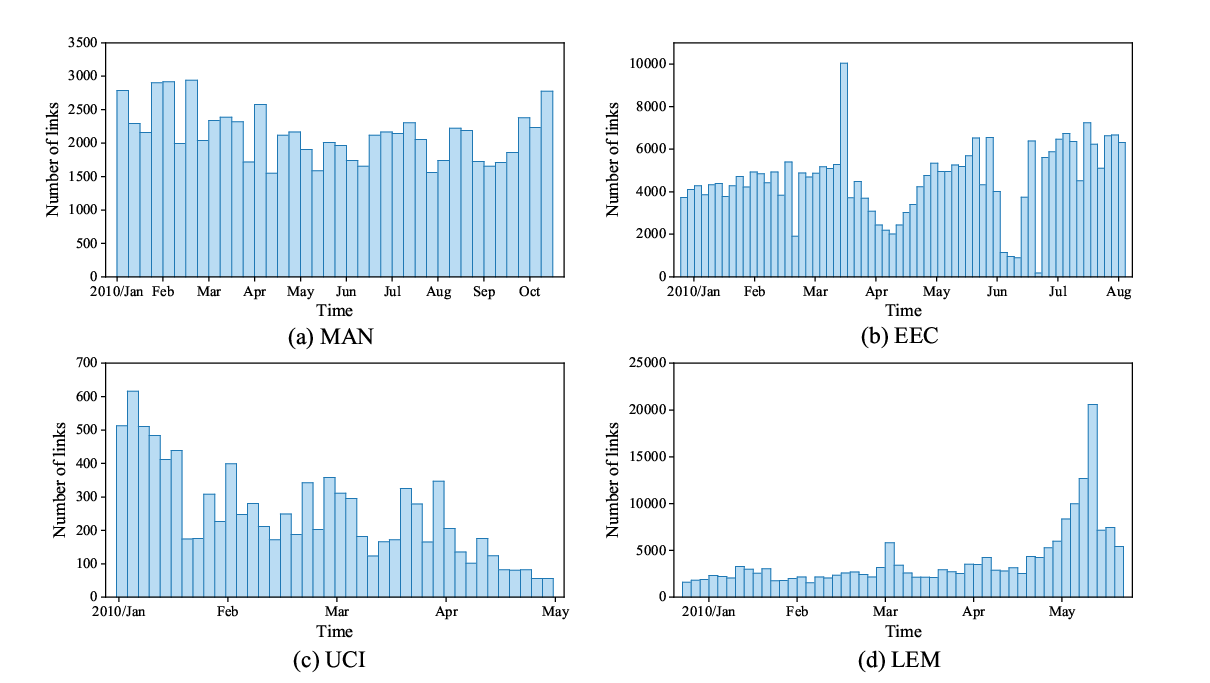
We use four temporal directed networks from real world to evaluate the performance of TSAM model, including two Email networks, a social network and an interaction network. Basic statistics of the four datasets are presented in Table 1, and a brief introduction of them is described as follows.

1. 1.

   Manufacturing emails (MAN) [27]: An email network between employees of a mid-sized manufacturing company. The network is directed and nodes represent employees. The left node represents the sender and the right node represents the recipient. A directed link $e(u,v,t)$ represents that employee $u$ sent an email to employee $v$ at time $t$. We use links in one week to generate a snapshot, and construct $38$ snapshots with total duration of $9$ months, as shown in Fig. 5(a).

2. 2.

   Email-Eu-core-temporal (EEC) [28]: An email network generated from the email data in a large European research institution. A directed link $e(u,v,t)$ represents that a person $u$ sent an email to another person $v$ at time $t$. The timestamp of this dataset starts from $0$ and no starting date is specified. We neglect the isolated links and only generate the snapshots based on links occurred during 15 consecutive months. Each snapshot contains links during one week, so we totally get $64$ snapshots as shown in Fig. 5(b).

3. 3.

   UC Irvine messages (UCI) [29]: A network consisted of private messages sent on an online social network at the University of California, Irvine. A directed link $e(u,v,t)$ represents that user $u$ sent a private message to user $v$ at time $t$. We choose links of 4 months in the experiments, and generate snapshots with the range of $3$ days as shown in Fig. 5(c).

4. 4.

   LevantMonths (LEM) [30]: An interaction network collected by the Kansas Event Data System based on folders containing WEIS-coded events within eight countries: Egypt, Israel, Jordan, Lebanon, Palestinians, Syria, USA, and Russia. The dataset contains interactions from April 1979 to June 2004. Each snapshot contains links occurred in $6$ months, and $50$ snapshots are constructed in total, as shown in Fig. 5(d).

We use two standard evaluation metrics to evaluate the performance of temporal link prediction models. The area under the receiver characteristic operator curve (AUC) is a widely adopted evaluation metric for classification models, which considers both the sensitivity and specificity of the model. In link prediction problems, if there are $n^{\prime}$ times that the scores of randomly chosen existent links are higher than those of randomly chosen non-existent links among $n$ independent comparisons, and $n^{\prime\prime}$ times that they get the same scores, then AUC is calculated as:

$$\mathrm{AUC}=\frac{n^{\prime}+0.5n^{\prime\prime}}{n}$$

(23)

A larger AUC score indicates a better prediction performance for a given model. Similar with AUC, the area under the precision-recall curve (PRAUC) is designed to evaluate the sparsity of networks. However, both AUC and PRAUC cannot evaluate the added and removed links at the same time. Therefore, in addition we adopt the geometric mean of AUC and PRAUC (GMAUC) [31] to evaluate both added and removed links, defined as:

$$\mathrm{GMAUC}=\left(\frac{\mathrm{PRAUC}-\frac{L_{A}}{L_{A}+L_{R}}}{1-L_{A}/(L_{A}+L_{R})}\cdot 2\left(\mathrm{AUC}-0.5\right)\right)^{1/2}$$

(24)

where $L_{A}$ and $L_{R}$ are the number of added and removed links respectively, $\mathrm{PRAUC}$ is the $\mathrm{PRAUC}$ value of new links, while $\mathrm{AUC}$ is the AUC score calculated by originally existed links.

Experiments are performed on a Ubuntu 16.04 LTS system with $48$ cores, $128$ GB RAM and $2.20$ GHz clock frequency. We implement the model in Tensorflow 1.15.0, and train it on a NVIDIA Titan Xp GPU. We use a sliding window with size $T$ to get continuous snapshot sequences from all snapshots in each network. At each time step $t$, we train separate models up to snapshot $t$ and evaluate it at $t+1$ for each $t=1,\cdots,T$.

We compare the performance of TSAM and five state-of-the-art models on temporal link prediction in directed networks, including:

1. 1.

   TNE [32]: It models the temporal network with Markov process and uses matrix factorization to learn node embeddings.

2. 2.

   GC-LSTM [11]: It is an end-to-end temporal link prediction model which uses GCN to extract structural features and LSTM to extract temporal features. We set the order of GCN $K=3$ to aggregate 3-hop neighbors.

3. 3.

   EvolveGCN [12]: It is a graph embedding model which adapts GCN model along the temporal dimension without resorting to node embeddings. It captures the dynamism of graph sequences using an RNN to evolve the GCN parameters.

4. 4.

   dyngraph2vec [33]: It uses multiple non-linear layers to learn structural patterns of each snapshot, and then uses recurrent layers to learn temporal transitions in the network. We choose one of its variations namely dyngraph2vetAERNN, which uses LSTM in the encoder to extract node embeddings and full-connected network in the decoder to generate predictions. The hyperparamerter $\mathrm{lb}$ is set to $T$.

5. 5.

   DySAT [7]: It is a graph embedding model based on joint self-attention along the two dimensions of structural neighborhood and temporal dynamics.

Notice that since we are dealing with directed networks, spectral domain convolution cannot perform on the asymmetric adjacency matrices because the asymmetric laplace matrices are not decomposable. Therefore, we replace all GCN units with GraphSAGE in GC-LSTM and EvolveGCN to perform spacial domain convolution on directed networks. The mean aggregator function is utilized in GraphSAGE to aggregate neighborhood features. Moreover, since TNE, EvolveGCN and DySAT are graph embedding models which learn node embedding $\mathbf{e}_{t}$ from the evolving network $G_{t-T}^{t}$, we define similarity score matrix $\mathbf{S}_{t+1}=\mathbf{e}_{t}\cdot\mathbf{e}_{t}^{\mathrm{T}}$ to use them for temporal link prediction task. In TSAM, we adopt four transformations $\{\mathbf{C}^{M_{1}},\mathbf{C}^{M_{2}},\mathbf{C}^{M_{3}},\mathbf{C}^{M_{4}}\}$ listed in (6) as additional feature inputs. Other parameter settings in four networks are presented in Table 2.

Table 3 and Table 4 presents the prediction performance of TSAM and baselines in four networks. From the results we can observe consistent gains of $1-2\%$ AUC in comparison to the best baseline in EEC, UCI and LEM. In MAN, the AUC of TSAM is slightly lower than DySAT, but TSAM get higher GMAUC than DySAT, which indicates a better performance of predicting both added and removed links. It is also clear that the performance of TSAM is more stable in four networks reflected by the smaller standard deviation. We also notice that compared with dyngraph2vec and GC-LSTM, our TSAM model and DySAT are able to achieve obvious improvements on both AUC and GMAUC, which indicates the effectiveness of self-attention mechanism on temporal link prediction task.

Fig. 6 presents the average AUC at each time step in four networks. We find that the performance of TSAM is relatively better and more stable than baselines. The superiority of TSAM is obvious in comparison with TNE and GC-LSTM, whose AUC curves show rapid drops at certain time steps.

An important improvement in TSAM compared with other baselines is the feature fusion block, which uses matrix transformation to capture motif features in directed networks. Here we analyze the influence of feature fusion block with different choices of additional feature. Table 5 and Table 6 present the performance of TSAM under three circumstances: 1) use only the output of GAT without additional features as the input of GRU, 2) use $\mathbf{C}^{M_{1}}$ as additional feature, 3) use matrices listed in Eq. (5) as additional feature. We adopt parameters under the best performance for each case. From the results we find that without additional feature, TSAM achieves lower AUC and GMAUC than DySAT in MAN and EEC. However, when $\mathbf{C}^{M_{1}}$ is adopted, an obvious improvement can be observed in four networks. Since $\mathbf{C}^{M_{1}}$ captures the local motifs of $u\to t\to v$, it indicates that taking into account the motif structure in directed networks can lead to improvement on prediction performance. We also find that with more additional features added, the performance of TSAM gets better, bringing along more computational costs at the same time.

Another important hyperparameter of TSAM is the number of attention heads in self-attention layers. Here we respectively analyze the influence of attention heads on the performance of TSAM. Fig. 7 presents the performance of TSAM when we independently vary the number of attention heads in node-level and time-level self-attention blocks within range $\{1,2,4,8,16\}$. In the results we find that more attention heads leads to better performance on both AUC and GMAUC. When $K_{N}\geq 4$ and $K_{T}\geq 8$, the performance tend to be stable. It indicates that it is efficient to capture latent features when using $4$ node-level attention heads and $8$ time-level attention heads.

References

- [1] Ravi Kumar, Jasmine Novak, and Andrew Tomkins. Structure and evolution of online social networks. In Proceedings of the 12th ACM SIGKDD international conference on Knowledge discovery and data mining - KDD ’06, pages 611–617, Philadelphia, PA, USA, 2006. ACM Press.
- [2] Kai Lei, Meng Qin, Bo Bai, Gong Zhang, and Min Yang. GCN-GAN: A non-linear temporal link prediction model for weighted dynamic networks. In IEEE INFOCOM 2019 - IEEE Conference on Computer Communications, pages 388–396, April 2019.
- [3] Linyuan Lü and Tao Zhou. Link prediction in complex networks: A survey. Phys. A, 390(6):1150–1170, March 2011.
- [4] Tomasz Tylenda, Ralitsa Angelova, and Srikanta Bedathur. Towards time-aware link prediction in evolving social networks. In Proceedings of the 3rd Workshop on Social Network Mining and Analysis - SNA-KDD ’09, pages 1–10, Paris, France, 2009. ACM Press.
- [5] David Liben-Nowell and Jon Kleinberg. The link-prediction problem for social networks. Journal of the American Society for Information Science and Technology, 58(7):1019–1031, May 2007.
- [6] Thomas N. Kipf and Max Welling. Semi-supervised classification with graph convolutional networks. In International Conference on Learning Representations, April 2017.
- [7] Aravind Sankar, Yanhong Wu, Liang Gou, Wei Zhang, and Hao Yang. DySAT: Deep Neural Representation Learning on Dynamic Graphs via Self-Attention Networks. In Proceedings of the 13th International Conference on Web Search and Data Mining, WSDM ’20, pages 519–527, Houston, TX, USA, January 2020. Association for Computing Machinery.
- [8] Ke-ke Shang, Michael Small, Xiao-ke Xu, and Wei-sheng Yan. The role of direct links for link prediction in evolving networks. EPL, 117(2):28002, January 2017.
- [9] Lekui Zhou, Yang Yang, Xiang Ren, Fei Wu, and Yueting Zhuang. Dynamic network embedding by modeling triadic closure process. In Thirty-second AAAI conference on artificial intelligence, 2018.
- [10] Palash Goyal, Nitin Kamra, Xinran He, and Yan Liu. DynGEM: Deep Embedding Method for Dynamic Graphs. arxiv, May 2018.
- [11] Jinyin Chen, Xuanheng Xu, Yangyang Wu, and Haibin Zheng. GC-LSTM: Graph Convolution Embedded LSTM for Dynamic Link Prediction. arxiv, December 2018.
- [12] Aldo Pareja, Giacomo Domeniconi, Jie Chen, Tengfei Ma, Toyotaro Suzumura, Hiroki Kanezashi, Tim Kaler, Tao B. Schardl, and Charles E. Leiserson. EvolveGCN: Evolving Graph Convolutional Networks for Dynamic Graphs. arxiv, February 2019.
- [13] Mujtaba Jawed, Mehmet Kaya, and Reda Alhajj. Time frame based link prediction in directed citation networks. In Proceedings of the 2015 IEEE/ACM International Conference on Advances in Social Networks Analysis and Mining 2015 - ASONAM ’15, pages 1162–1168, Paris, France, 2015. ACM Press.
- [14] Ertan Bütün, Mehmet Kaya, and Reda Alhajj. Extension of neighbor-based link prediction methods for directed, weighted and temporal social networks. Information Sciences, 463-464:152–165, October 2018.
- [15] William L. Hamilton, Rex Ying, and Jure Leskovec. Inductive representation learning on large graphs. arxiv, June 2017.
- [16] Manoj Reddy Dareddy, Mahashweta Das, and Hao Yang. Motif2vec: Motif aware node representation learning for heterogeneous networks. August 2019.
- [17] Zekarias T. Kefato, Nasrullah Sheikh, and Alberto Montresor. Which way? Direction-Aware Attributed Graph Embedding. arxiv, January 2020.
- [18] Jiankai Sun, Bortik Bandyopadhyay, Armin Bashizade, Jiongqian Liang, P. Sadayappan, and Srinivasan Parthasarathy. ATP: Directed Graph Embedding with Asymmetric Transitivity Preservation. arxiv, November 2018.
- [19] Federico Monti, Karl Otness, and Michael M. Bronstein. MotifNet: A motif-based graph convolutional network for directed graphs. In 2018 IEEE Data Science Workshop (DSW), pages 225–228, Lausanne, Switzerland, June 2018. IEEE.
- [20] Petar Veličković, Guillem Cucurull, Arantxa Casanova, Adriana Romero, Pietro Liò, and Yoshua Bengio. Graph attention networks. arxiv, October 2017.
- [21] Weiwei Gu, Fei Gao, Xiaodan Lou, and Jiang Zhang. Link prediction via graph attention network. arXiv, October 2019.
- [22] Jiani Zhang, Xingjian Shi, Junyuan Xie, Hao Ma, Irwin King, and Dit-Yan Yeung. GaAN: Gated Attention Networks for Learning on Large and Spatiotemporal Graphs. arXiv, March 2018.
- [23] Ginestra Bianconi, Natali Gulbahce, and Adilson E. Motter. Local structure of directed networks. Phys. Rev. Lett., 100(11), March 2008.
- [24] Ashish Vaswani, Noam Shazeer, Niki Parmar, Jakob Uszkoreit, Llion Jones, Aidan N. Gomez, Lukasz Kaiser, and Illia Polosukhin. Attention Is All You Need. arxiv, June 2017.
- [25] Elena Voita, David Talbot, Fedor Moiseev, Rico Sennrich, and Ivan Titov. Analyzing Multi-Head Self-Attention: Specialized Heads Do the Heavy Lifting, the Rest Can Be Pruned. arxiv, May 2019.
- [26] Daixin Wang, Peng Cui, and Wenwu Zhu. Structural Deep Network Embedding. In Proceedings of the 22nd ACM SIGKDD International Conference on Knowledge Discovery and Data Mining, KDD ’16, pages 1225–1234, San Francisco, California, USA, August 2016. Association for Computing Machinery.
- [27] Jérôme Kunegis. KONECT: the Koblenz network collection. In Proceedings of the 22nd International Conference on World Wide Web - WWW ’13 Companion, pages 1343–1350, Rio de Janeiro, Brazil, 2013. ACM Press.
- [28] Ashwin Paranjape, Austin R. Benson, and Jure Leskovec. Motifs in Temporal Networks. In Proceedings of the Tenth ACM International Conference on Web Search and Data Mining - WSDM ’17, pages 601–610, Cambridge, United Kingdom, 2017. ACM Press.
- [29] Pietro Panzarasa, Tore Opsahl, and Kathleen M. Carley. Patterns and dynamics of users’ behavior and interaction: Network analysis of an online community. J. Am. Soc. Inf. Sci. Technol., 60(5):911–932, May 2009.
- [30] Jure Leskovec and Andrej Krevl. SNAP Datasets: Standford large network dataset collection, January 2014.
- [31] R. R. Junuthula, K. S. Xu, and V. K. Devabhaktuni. Evaluating link prediction accuracy in dynamic networks with added and removed edges. In 2016 IEEE International Conferences on Big Data and Cloud Computing (BDCloud), Social Computing and Networking (SocialCom), Sustainable Computing and Communications (SustainCom) (BDCloud-SocialCom-SustainCom), pages 377–384, 2016.
- [32] Linhong Zhu, Dong Guo, Junming Yin, Greg Ver Steeg, and Aram Galstyan. Scalable Temporal Latent Space Inference for Link Prediction in Dynamic Social Networks. IEEE Trans. Knowl. Data Eng., 28(10):2765–2777, October 2016.
- [33] Palash Goyal, Sujit Rokka Chhetri, and Arquimedes Canedo. dyngraph2vec: Capturing Network Dynamics using Dynamic Graph Representation Learning. arxiv, September 2018.