Ptolemy: Architecture Support for Robust Deep Learning
Abstract
Deep learning is vulnerable to adversarial attacks, where carefully-crafted input perturbations could mislead a well-trained Deep Neural Network (DNN) to produce incorrect results. Adversarial attacks jeopardize the safety, security, and privacy of DNN-enabled systems. Today’s countermeasures to adversarial attacks either do not have the capability to detect adversarial samples at inference-time, or introduce prohibitively high overhead to be practical at inference-time.
We propose Ptolemy, an algorithm-architecture co-designed system that detects adversarial attacks at inference time with low overhead and high accuracy. We exploit the synergies between DNN inference and imperative program execution: an input to a DNN uniquely activates a set of neurons that contribute significantly to the inference output, analogous to the sequence of basic blocks exercised by an input in a conventional program. Critically, we observe that adversarial samples tend to activate distinctive paths from those of benign inputs. Leveraging this insight, we propose an adversarial sample detection framework, which uses canary paths generated from offline profiling to detect adversarial samples at runtime. The Ptolemy compiler along with the co-designed hardware enable efficient execution by exploiting the unique algorithmic characteristics. Extensive evaluations show that Ptolemy achieves higher or similar adversarial sample detection accuracy than today’s mechanisms with a much lower (as low as 2%) runtime overhead.
Index Terms:
DNN; Robustness; Deep learning; Adversarial Attack; Adversarial Samples; Defense;I Introduction
Deep Neural Networks (DNN) are not robust. Small perturbations to inputs could easily “fool” DNNs to produce incorrect results. By manipulating the perturbation, a range of so-called adversarial attacks have been demonstrated to lead DNNs to mis-predict [53, 13, 36, 66, 50, 28], which could result in potentially severe consequences. For instance, physically putting a sticker on a stop sign could lead a well-trained object recognition DNN to misclassify the stop sign as a yield sign [36]. Beyond mission-critical scenarios such as autonomous driving, the robustness issue also obstructs the deployment of DNN in privacy/security-sensitive domains such as biometric authentication [54, 63].
We take a first step toward architectural support for robust deep learning. For a robustness scheme to be effective in practice, it not only has to accurately detect adversarial inputs, but must also do so efficiently at inference time so that proper measure could be taken. This paper proposes Ptolemy, an algorithm-architecture co-design system that detects adversarial attacks at inference time with low overhead and high accuracy. This enables applications to reject incorrect results produced by adversarial attacks during inference. Fig. 1 provides an overview of the system.
Existing countermeasures to adversarial attacks are unable to detect adversarial samples at inference time [12, 25]. Fundamentally, they treat DNN inferences as black boxes, ignoring their runtime behaviors. To enable efficient online adversarial detection, this paper takes a different, white-box approach. We exploit the fact that each input to a DNN uniquely exercises an activation path—a collection of neurons that contribute significantly to the inference output, analogous to the sequence of basic blocks exercised by an input in a conventional program. Analyzing “hot” activation paths in DNNs, our key observation is that inputs that lead to the same inference class tend to exercise a group of paths that are distinctive from other inference classes.

We propose a general algorithmic framework that exploits the runtime path behaviors for efficient online adversarial sample detection. The detection framework constructs a canary class path offline for each inference class by profiling the training data. At runtime, it builds the activation path for an input, and detects the input as an adversary if the activation path is different from the canary path associated with the predicted class. The general algorithm framework exposes a myriad of design knobs affecting the critical trade-off between detection accuracy and compute cost, such as how a path is formulated and when the path is constructed. To widen the applicability of our detection framework, Ptolemy provides a high-level programming interface, which allows programmers to calibrate the algorithmic knobs to explore the accuracy-cost trade-off that best suits an application’s needs.
Ptolemy provides an efficient execution substrate. The key to the execution efficiency is the Ptolemy compiler, which hides and reduces the detection overhead by exploiting the unique parallelisms and redundancies exposed by the detection algorithms. We show that with the aggressive compile-time optimizations and a well-defined ISA, detection algorithms can be implemented on top of existing DNN accelerators with a set of basic, yet principled, hardware extensions, further widening the applicability of Ptolemy.
Ptolemy enables highly accurate adversarial detection with low performance overhead. Compared to today’s defense mechanisms that introduce over 10 performance overhead, we demonstrate a system that achieves higher accuracy with only 2% performance overhead. Ptolemy defends not only existing attacks, but also adaptive attacks that are specifically designed to defeat our defense [11]. We also demonstrate the Ptolemy framework’s flexibility by presenting a range of algorithm variants that offer different accuracy-efficiency trade-offs. For instance, Ptolemy could trade 10% performance overhead for 0.03 higher detection accuracy.
The Ptolemy artifact, including the pre-trained models, offline-generated class paths, code to generate adaptive and non-adaptive attacks, and the detection implementation is available at https://github.com/Ptolemy-DL/Ptolemy. In summary, Ptolemy provides a generic framework for low-overhead, high-accuracy online defense against adversarial attacks with the following contributions:
- •
We propose a novel static-dynamic collaborative approach for adversarial detection by exploiting the unique program execution characteristics of DNN inferences that are largely ignored before.
- •
We present a general algorithmic framework, along with a high-level programming interface, that allows programmers to explore key algorithm design knobs to navigate the accuracy-efficiency trade-off space.
- •
We demonstrate that with a carefully-designed ISA, compiler optimizations could enable efficient detection by exploiting the unique parallelisms and redundancies exposed by our detection algorithm framework.
- •
We present a programmable hardware to achieve low-latency online adversarial defense with principled extensions to existing DNN accelerators.
II Background
Adversarial Attacks
DNNs are not robust to adversarial attacks, where DNNs mis-predict under slightly perturbed inputs [13, 36, 53, 47]. Fig. 2 shows one such example, where the two slightly different images are both perceived as stop signs to human eyes, but the second image is mis-predicted by a DNN model as a yield sign. The perturbations could be the result of carefully engineered attacks, but could also be an artifact of normal data acquisition such as noisy sensor capturing and image compression/resizing [67].
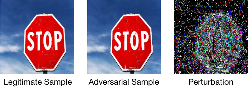
Formally, given a DNN , an input is defined as an adversarial sample if it is close to yet makes , where is the correct class of . Different adversarial samples differ in their measures of the distance between and . The distance could be small, where the input perturbations are imperceptible to humans (as in the example above), but could also be large, where the perturbations are visible to humans but still “fool” a DNN. For instance, physically putting a sticker on a stop sign could mislead a DNN to misclassify the stop sign as a yield sign [36, 40]. Ptolemy targets the general robustness issue that introduces mis-predictions through input perturbations—small or large, inadvertent or malicious. For simplicity, we refer to all of them as adversarial attacks throughout this paper.
An adversarial attack is a black-box attack if it does not assume knowledge of the attacked model; white-box attacks in contrast assume full knowledge of the model. Orthogonally, adaptive attacks have complete knowledge of the defense’s inner workings, i.e., are specifically designed to attempt to defeat a defense, while non-adaptive attacks do not [68, 11, 12]. We show that our detection scheme can defend against a range of different attacks, including the strongest form of attack: white-box adaptive attacks.
Countermeasures
We aim to enable fast and accurate systems that can detect adversarial examples at inference-time such that proper measures could be taken. Today’s defense mechanisms largely fall under two categories, neither of which meets this goal. The first class of defenses improves the robustness of DNN models at training time (e.g., adversarial retraining) [69, 75] by incorporating adversarial examples into the training data. However, re-training is not suitable at inference-time and requires accesses to the training data. Another class of defenses uses redundancies to defend against adversarial attacks [67, 57], similar to the multi-module redundancy used in classic fault-tolerant systems [62]. This scheme, however, introduces high overhead, limiting its applicability at inference time.
III Algorithmic Framework
This section introduces the Ptolemy algorithm framework, which enables adversarial attack detection at inference-time with high accuracy and low latency. Ptolemy provides a set of principled design knobs to allow programmers to customize the accuracy vs. efficiency trade-off.
We first describe the intuition and key concepts behind our algorithm framework (Sec. III-A). We then introduce the algorithm framework, and show that a basic algorithm under the framework introduces excessive compute and memory cost (Sec. III-B). We further introduce key algorithmic knobs that enable different algorithm variants to offer different accuracy-efficiency trade-offs (Sec. III-C). Finally, we introduce a high-level programming interface to flexibly express detection algorithms within our framework (Sec. III-D).
III-A Intuition and Key Concepts
Intuition
Each input to a DNN activates a sequence of neurons. We find that inputs that are correctly predicted as the same class tend to activate a unique set of neurons distinctive from that of other inputs. This is a manifestation of recent work on class-level model sparsity [55, 72], which shows that a small, but distinctive, portion of the network contributes to each predicted class. Taking this perspective, the way adversarial samples alter the inference result can be thought of as activating a sequence of neurons different from the canonical sequence associated with its predicted output. Analyzing dynamic paths in DNN inferences thus allows us to detect adversaries.
A sequence of activated neurons is analogous to a sequence of basic blocks exercised by an input to a conventional program. The frequently exercised basic block sequences, i.e., “hot paths” [7, 20, 15], can be used to improve performance in classic profile-guided optimizations and dynamic compilers [60, 59, 19]. Our approach shares a similar idea, where we treat a DNN as an imperative program, and leverage its runtime paths (sequence of neurons) to guide adversarial sample detection. Conventional countermeasures largely ignore the program execution behaviors of DNN inferences.

Important Neurons
The premise of our detection algorithm framework is the notion of important neurons, which denote a set of neurons that contribute significantly to the inference output. Important neurons are extracted in a backward fashion. The last layer has only one important neuron, which is the neuron that corresponds to the predicted class. At the second last layer , the important neurons are the minimal set of neurons in the input feature map that contribute to at least () of . Here, controls the coverage of important neurons. To extract the important neurons of layer , we simply rank the partial sums used to calculate , and choose the minimal number of neurons whose partial sums collectively contribute to at least .
The left panel in Fig. 3 shows an example using a fully-connected layer. Assuming and the second neuron in the output feature map (0.46) is the important neuron identified in the next layer. The fourth (1.0) and the fifth (0.1) neurons in the input feature map are identified as the important neurons in the current layer, because they contribute the two large partial sums and their cumulative partial sum (0.3) contribute to more than 60% of the important neuron in the output feature map. The same process can be extended to convolution layers. The middle panel in Fig. 3 shows an example. For the important neuron in the output feature map, we first find its receptive field in the input feature map, and then identify the minimal set of neurons in the receptive field whose cumulative partial sums contribute to at least .
This process is repeated backwards from the last layer to the first layer, as shown in the right panel in Fig. 3. The important neurons identified at layer are used to determine the important neurons at layer .


From Neurons to Paths
The collection of important neurons across all the layers under a given input constitutes an activation path of that input, similar to how a sequence of basic blocks constitutes a path/trace in a program. We represent a path using a bitmask, where each bit indicates whether the neuron (input feature map element) at layer position is an important neuron.
From individual activation paths, we introduce the concept of a class path for a class , which aggregates (bitwise OR) the activation paths of different inputs that are correctly predicted as class . That is: , where denotes the activation path of input , denotes the set of all the correctly predicted inputs of class , denotes bitwise OR, and denotes the class path of class . We observe that starts to saturate around 100 images and including more images from the training dataset does not result all bits being 1. We do not manually stop filling the bits.
Critically, class paths are significantly different from each other. Fig. 5a shows the path similarity in AlexNet [35] across 10 randomly-sampled classes from ImageNet [17]. Fig. 5b shows the path similarity in ResNet18 [64] across the 10 classes in CIFAR-10 [34]. All the results are obtained on the training set. The average inter-class path similarity is only 36.2% (max 38.2%, 90-percentile 36.6%) for AlexNet on ImageNet and 61.2% (max 65.1%, 90-percentile 63.4%) for ResNet18 on CIFAR-10, suggesting that class paths are distinctive. In an attempt to normalize the dataset, we also perform the same experiment on ResNet50 on ImageNet. The average inter-class path similarity is 37.6% (max 40.9%, 90-percentile 39.1%), similar to those of AlexNet on ImageNet.
The class path similarity is much higher in CIFAR-10 than in ImageNet. This is because ImageNet has 1,000 classes that cover a wide range of objects and CIFAR-10 has only 10 classes, which are similar to each other (e.g., cat vs. dog). The randomly picked 10 classes in ImageNet are more likely to be different from each other than the 10 classes in CIFAR-10. Across all the 1,000 classes in ImageNet, the maximum inter-class path similarity is still only 0.44, suggesting that our random sampling of ImageNet is representative.
III-B Detection Framework and Cost Analysis
We leverage the clear distinction across different class paths to detect adversarial inputs. If an input is predicted as class while its activation path does not resemble the class path , we hypothesize that the input is an adversary.
Framework
Fig. 4 shows an overview of the algorithm framework, which requires static-dynamic collaboration. The static component profiles the training data to extract activation paths for each correctly predicted sample , and generates the class path for each class as described before. The class paths are stored offline and reused over time. Critically, our profiling method can easily integrate new training samples, whose activation paths would simply be aggregated (OR-ed) with the existing class paths without having to re-generate the entire class paths from scratch.
At inference-time, the dynamic component extracts the path for a given input. Note that activation paths are extracted only after the entire DNN inference finishes, because the identification of important neurons starts from the predicted class in the last layer and propagates backward. We will show other variants in Sec. III-C that relax this restriction.
Given the activation path of an input and the canary class path , where is the predicted class of , a classification module then decides whether is an adversary or not based on the similarity between and . While a range of similarity metrics and algorithms could be used, we propose a lightweight algorithm that is extremely efficient to compute while providing high accuracy. Specifically, we first estimate the similarity between and : , where denotes the number of 1s in the vector , and denotes bitwise AND. is fed into a learned classifier, for which we use the lightweight random forest method [41], for the final classification. The classification module is lightweight, contributing to less than 0.1% of the total detection cost.
Cost Analysis
The algorithm described above is able to achieve accuracy higher than state-of-the-art methods (see Sec. VII). However, runtime extraction of activation paths also introduces significant memory and compute costs.
The memory cost is significant because every single partial sum generated during inference must be stored in the memory before the path extraction process begins. The detection algorithm introduces 9 to 420 memory overhead, which is a lower bound of the actual memory traffic overhead in real systems because the massive partial sums will not be buffered completely on-chip. Storing partial sums will also stall the computing units and increase latency.
Path extraction also introduces compute overhead due to sorting and accumulating partial sums. Using AlexNet as an example, at , the compute overhead could be as high as 30%. At first glance, it might be surprising that the compute overhead is “only” 30%. Further investigations show that percentage of important neurons in a network is generally below 5% even with . Thus, the expensive sorting and accumulation operations are applied to only a small portion of partial sums. Note that the compute cost shown here leads to much higher latency overhead in reality because, while inference is massively parallel, sorting and accumulating are much less so. A pure software implementation of the detection algorithm introduces 15.4 and 50.7 overhead over inference on AlexNet and ResNet50, respectively.
III-C Algorithmic Knobs and Variants
To trade little accuracy loss for significant efficiency gains, we introduce three algorithmic knobs that control how activation paths are extracted, which dominates the runtime performance/energy overhead. The result is a set of algorithm variants that follow the same algorithm framework described in Fig. 4, but that differ in how the paths are extracted.
Hiding Detection Cost: Extraction Direction
The cost introduced by the basic detection algorithm directly increases the inference latency because path extraction and inference must be serialized. We identify a key algorithmic knob that provides the opportunity to hide the compute cost of detection by overlapping detection with inference.
The key to the new algorithm is to extract important neurons in a forward rather than a backward manner. Recall that in the original backward extraction process, we use the important neurons in layer ’s output (which is equivalent to layer ’s input) to identify the important neurons in layer ’s input. In our new forward extraction process, as soon as layer finishes inference we first determine the important neurons in its output by simply ranking output neurons according to their numerical values and selecting the largest neurons, instead of waiting until after the extraction of layer . In this way, the extraction of important neurons at layer and the inference of layer can be overlapped.
Reducing Detection Cost: Thresholding Mechanism
The forward extraction process hides the extraction behind inference, but does not reduce the detection cost, which could significantly increase the energy overhead.
To reduce the detection cost, we propose to extract important neurons using absolute thresholds rather than cumulative thresholds. Whenever a partial sum is generated during inference it is compared against an absolute threshold . A single-bit mask is stored to the memory based on the comparison result. Later during path extraction, the masks (as opposed to partial sums) are loaded to determine important neurons. Thresholding can be specified at each layer, and can be applied to both extraction directions.
Using absolute thresholds significantly reduces both the compute and memory costs (Sec. VII-C), because comparing partial sums against a threshold is much cheaper than sorting and accumulating them, and writing single-bit masks rather than partial sums significantly reduces the memory accesses.
Reducing Detection Cost: Selective Extraction
An orthogonal way to reduce the cost is to skip important neurons from certain layers altogether. In many networks, later layers have a more significant impact on the inference output than earlier layers [56]. Thus, one could extract important neurons from just the last a few layers to further reduce the cost (Sec. VII-F). When combined with forward extraction, this is equivalent to starting extraction later (“late-start”); when combined with backward extraction, this is equivalent to terminating extraction earlier (“early-termination”). This knob specifies the start/termination layer.
Summary
The Ptolemy framework provides three different knobs to explore the accuracy-efficiency trade-off. While the extraction direction applies to the entire network and hides the detection cost behind the inference cost, the thresholding mechanism and the extracted layer are specified at the layer level to reduce the detection cost.
| Class | Name | 23-20 | 19-16 | 15-12 | 11-8 | 7-4 | 3-0 |
|---|---|---|---|---|---|---|---|
| Inference | inf | 0000 | Input addr. | Weight addr. | Output addr. | Unused | |
| infsp | 0001 | Input addr. | Weight addr. | Output addr. | First partial sum addr. | Unused | |
| csps | 0010 | Output neuron ID | Layer ID | First partial sum addr. | Unused | ||
| Path Construction | sort | 0011 | Unsorted seq. start addr. | Seq. length | Sorted seq. start addr. | Unused | |
| acum | 0100 | Input addr. | Output addr. | Cumulative threshold | Unused | ||
| genmasks | 0101 | Input addr. | Output addr. | Unused | |||
| findneuron | 0110 | Layer ID | Neuron position | Target neuron addr. | Unused | ||
| findrf | 0111 | Neuron addr. | Receptive field addr. | Unused | |||
| Classification | cls | 1000 | Class path addr. | Activation path addr. | Result | Unused | |
| Others | Omitted for simplicity (mov, dec, jne, etc.) | ||||||
III-D Programming Interface
Ptolemy provides a (Python-based) programming interface that allows programmers to express a range of different algorithmic design knobs described above. Our programming interface is designed with two principles in mind, which we will explain using an actual detection algorithm expressed using the programming interface shown in Fig. 6.
Decoupled Inference/Detection
The Ptolemy programming interface decouples inference with detection, which allows programmers to focus on expressing the functionalities of the detection algorithm while leaving optimizations to the compiler and runtime. For instance, while the inference code (Line 2) and the path extraction code (Line 3–15) are expressed sequentially in the program, our compiler will understand that the program uses the forward extraction algorithm (Line 8 and 11), and thus will automatically pipeline inference with important neuron extraction across layers (see Sec. IV-B).
Per-Layer Extraction Granularity
Our programming interface provides the flexibility to specify the important neuron extraction method for each layer to leverage the three knobs described above to explore the efficiency-accuracy trade-off space. We will demonstrate its effectiveness in Sec. VII-F.
For instance in Fig. 6, the programmer selectively extracts important neurons only for the last three layers (Line 5). In addition, only the last layer uses the cumulative threshold to extract important neurons (Line 11), which is more accurate but requires more computations than using absolute thresholds, which is the method used by the other two layers (Line 8). Note that we do not allow backward extraction and forward extraction to be combined in one network to avoid discrepancies in the layer where they join.
IV ISA and Compiler Optimizations
This section describes how Ptolemy efficiently maps detection algorithms expressed in the high-level programming interface to the hardware architecture. To that end, we first introduce the software-hardware interface, i.e., the Instruction Set Architecture (ISA) (Sec. IV-A), followed by the compiler optimizations (Sec. IV-B).
IV-A Instruction Set Architecture
Ptolemy provides a custom CISC-like ISA to allow efficient mapping from high-level detection algorithms to the hardware architecture. The design principles of the ISA are two-fold. First, it abstracts away hardware implementation details; the semantics are closer to high-level DNN programmers, and the instructions will be decomposed by micro-instructions controlled by an FSM. Second, it exposes opportunities for compiler and hardware to exploit parallelisms.
The Ptolemy ISA contains four types of instructions: Inference, Path Construction, Classification, and Others. They are high-level instructions in the CISC style that perform complex operations. We use a 24-bit fixed length encoding, and provide 16 general-purpose registers. Table I summarizes the instructions. We highlight key design decisions.
- •
Inference These instructions dictate the inference process. In addition to support usual inferences (inf), Ptolemy also provides an instruction that stores the partial sums to memory (infsp) during inference for backward extraction. Each inference instruction operates on one layer to match the per-layer extraction semantics in the high-level programming interface. Finally, the ISA also provides a special instruction that calculates and stores all the partial sums given an output feature map element (csps), which will be used by the compiler for memory optimizations.
- •
Path Construction This class of instructions is used to construct activation path dynamically at runtime for any given input. To construct path, the ISA provides instructions to identify important neurons (sorting sort, accumulate acum) and to generate the masks from the identified important neurons to form an activation path (genmasks). There are also instructions to calculate neuron addresses, which are convenient in finding the start address of a receptive field for a given neuron (findrf) and finding a given neuron given its position in the network (findneuron).
- •
Classification The classification instruction (cls) is used to classify an input as either adversarial or benign.
- •
Others The ISA provides a set of control-flow instructions (e.g., and jne), arithmetic instructions (e.g., dec), and scalar data movement instructions (e.g., mov).
Example
Lst. 1 shows a sample code that uses cumulative thresholds to extract important neurons. Through a loop, it iteratively finds a receptive field (findrf), sorts partial sums in the receptive field (sort), and uses the sorted partial sums to identify important neurons whose cumulative partial sums exceed the threshold (acum).
It highlights an important design decision of the Ptolemy ISA: all the detection related instructions use register operands. This design simplifies instruction encoding with little performance impact. For instance, the findrf instruction requires the receptive field size as an operand, which can be statically calculated by the compiler given the DNN model configurations. Since the receptive field size could be arbitrarily large and thus does not always fit in a reasonable, fixed-length encoding, a mov instruction is used to move the statically calculated immediate value to a register (r3), which is later used in the sort instruction. While a more complex instruction encoding that limits the range of immediate operands could eliminate this mov instruction, the performance overhead introduced by this mov instruction is negligible compared to the heavy-duty sort and acum instructions.
IV-B Code Generation and Optimization
The compiler maximizes performance by exploiting unique parallelisms and redundancies inherent to the detection algorithms. This is achieved through statically scheduling instructions, which minimizes runtime overhead and hardware complexity. Static scheduling is possible because the compute and memory access behaviors of both DNN inference and detection are known at the compile time.
Layer-Level Pipelining
A key characteristic of algorithms that use the forward extraction method is that inference and extraction of different layers can be overlapped. While the high-level programming interface decouples inference (Inference) and extraction (ExtractImptNeurons), and expresses them sequentially, our compiler will reorder instructions to enable automatic pipelining at runtime, in a way similar to classic software-pipelining technique [5].
Fig. 7a shows an example. We use pseudo-code to remove unnecessary details. <extraction for j> indicates the code block for extracting important neurons at layer j, and inf(j) indicates inference at layer j. By simply reordering instructions, inference of layer j+1 and extraction of layer j, which are independent, could be pipelined. At the hardware level, once inf(j) is issued to execute on the DNN accelerator, <extraction for j> could be issued and executed immediately on our hardware extension (Sec. V-B).
Note that our software pipelining technique does not fully hide the instruction latency to guarantee that a new instruction can be dispatched every cycle. Both inference and the extraction code block take tens of millions of cycles. Fully hiding latencies requires expensive optimizations in classic compiler literature [70, 27]. We find that our simple static instruction reordering is able to largely overlap inference with extraction, leading to very low performance overhead. A side effect of not fully hiding the instruction latencies is that our hardware would still have the logic to check dependencies and stall the pipeline if necessary. But the hardware remains in-order without the expensive out-of-order instruction scheduling logic.
Neuron-Level Pipelining
Similar to layer-level pipelining, our compiler will also automatically pipeline the extraction of different important neurons within a layer. Fig. 7b shows an example, where cumulative thresholds are used. The two steps needed to extract important neurons, sorting all the partial sums (sort) and accumulating the partial sums until the threshold is reached (acum), have data dependencies. The compiler overlaps the extraction across different important neurons (iterations), improving hardware utilization and performance.
Trading-off Compute for Memory
Algorithms that use cumulative thresholds have high memory cost because all the partial sums must be stored to memory (Fig. 5). However, if a receptive field does not correspond to an important neuron in the output feature map, its partial sums will not be used later. We observe that fewer than 5% of the partial sums stored are used later to extract important neurons.
We propose to use redundant computation to reduce memory overhead. Instead of storing all the partial sums during inference, we re-compute the partial sums during the extraction process only for the receptive fields that are known to correspond to important neurons in the output feature map. The compiler implements this by generating csps instructions to re-compute partial sums.
V Architecture Support
This section introduces the Ptolemy hardware architecture. Following an overview (Sec. V-A), we describe the designs of major hardware components (Sec. V-B – Sec. V-D).
V-A Overview
Our architecture builds on top of a conventional DNN accelerator. Fig. 8 provides an overview of the Ptolemy architecture, which consists of an augmented DNN accelerator, a Path Constructor that builds the activation path for an input, and a Controller that dispatches instructions, runs state machines that control the hardware blocks, and executes the final classifier. An off-chip memory stores all the data structures that are needed for inference and detection. Both the DNN accelerator and the Path Constructor use double-buffered on-chip SRAMs to capture data reuse and to overlap DMA transfer with computation. The controller’s SRAM stores the compiled detection program and activation/class paths for classification.
V-B Enhanced DNN Accelerator
Ptolemy can be integrated into general DNN accelerator designs. Without losing generality we assume a TPU-like systolic array design [31]. Each PE consists of two 16-bit input registers, a 16-bit fixed-point MAC unit with a 32-bit accumulator register, and simple trivial control logic.
Ptolemy minimally extends each MAC unit. Fig. 9a shows the simple MAC unit augmentations (shaded). Specifically, algorithms that use absolute thresholds compare each partial sum with the threshold and store the single-bit mask to the SRAM; algorithms that use cumulative thresholds require each partial sum to be stored to the SRAM. Note that with the re-computation optimization, partial sums are recomputed at extraction time only for important neurons instead of being stored during inference.
To avoid the SRAM becoming a scalability bottleneck, the partial sums and the masks are double-buffered in the SRAM and doubled-buffered to the DRAM through a DMA. Later, the partial sums and/or masks are double-buffered back to the SRAM, similar to how feature maps and kernels are accessed. The extra DRAM space required to store partial sums is small as we will show in Sec. VII-A. The additional DRAM traffic incurred by storing and reading partial sums is negligible (0.1%) compared to the original DRAM traffic since each partial sum is read and stored only once.
The PE array is used both for the usual inference and for re-computing partial sums as instructed by the clps instruction (Sec. IV-B). During re-computation, only the first row in the PE array is active because only a selected few elements in the output feature maps are to be re-computed.
V-C Path Constructor
The goal of the path constructor is to extract important neurons and to construct activation paths. Algorithms that use cumulative thresholds requires sorting partial sums in receptive fields. Since receptive fields in modern DNNs are usually large (tens of thousands of elements), sorting all the elements on one piece of hardware could become a latency bottleneck as the sequence length increases. Our design splits a long sequence into multiple subsequences, which are sorted in parallel and merged together. Fig. 9b shows the sort unit organization. The sort unit uses the classic sorting network [32], and the merge unit uses a standard merge tree, both have efficient hardware implementations [48, 16, 33].
The path constructor uses lightweight mask generation hardware, which generates the important neuron masks for each layer, from which the entire activation path (a bit vector) is constructed. The path constructor also integrates hardware that calculates similarities between an activation path and a canary class path, which is a highly bit-parallel operation. The SRAM in the path constructor is separate from the SRAM used by the DNN accelerator to avoid resource contention, and is also doubled-buffered.
V-D Controller
We assume a micro-controller unit (MCU) in the baseline hardware, as is common in today’s DNN-based Systems-on-a-chip (SoCs) [2]. We piggyback two key tasks on the MCU: dispatching instructions and executing the final classifier to detect adversaries. Both are lightweight tasks that can be executed efficiently on an MCU without extra hardware.
Dispatching Instructions
Thanks to the simple ISA encoding (Table I), the compiled programs can be interpreted on the MCU (i.e., software decoding) efficiently while avoiding extra hardware cost. The overhead of interpreting the code is negligible compared to the total execution time. The programs are very small in size. The largest one, which uses cumulative thresholds and backward extraction, is about 30 static instructions (below 100 bytes).
Classification
The similarity between an activation path and the canary class path calculated from the path constructor is fed into a random forest (RF) for the final classification (Sec. III-B). Our particular RF implementation uses 100 decision trees, each of which has an average depth of 12. In total, RF consumes about 2,000 operations on AlexNet (five orders of magnitude lower than inference), and could execute on an MCU in microseconds.
VI Evaluation Methodology
This section explains the basic hardware and software setup (Sec. VI-A) and the evaluation plan (Sec. VI-B).
VI-A Experimental Setup
Hardware Implementation We develop RTL implementation using Synposys synthesis and Cadence layout tools with Silvaco’s Open-Cell 15nm technology [1]. The on-chip SRAM is generated using an ARM memory compiler and the off-chip DRAM is modeled after four Micron 16 Gb LPDDR3-1600 channels. We assume an ARM Cortex M4-like micro-controller (MCU) as the controller in the hardware (Sec. V-D). The synthesis and memory estimation results are used to drive a cycle-level simulator for performance and energy analyses.
Networks and Datasets We evaluate Ptolemy using two networks: 1) ResNet18 [64] on the CIFAR-100 dataset [34] with 100 different classes and 50,000 training images, and 2) AlexNet [35] on the ImageNet dataset [17] with 1000 different classes and 1 million training images. The networks and datasets we evaluate are at the high end of the benchmark scale evaluated by today’s countermeasure mechanisms [12, 25, 45], which mostly use much smaller datasets and networks (e.g., MNIST, CIFAR-10) [37, 49] that are less effective in exercising the capability of our system. The test sets are evenly split between adversarial and benign inputs, following the common setup of adversarial attack research.
The clean AlexNet without attacks has an accuracy of 55.13% on ImageNet; ResNet18 has an accuracy of 94.49% and 75.87% on CIFAR-10 and CIFAR-100, respectively.
Attacks We evaluate Ptolemy against a wide range of attacks. We first evaluate using five common non-adaptive attacks: BIM [36], CWL2 [14], DeepFool [47], FGSM [52], and JSMA [52], which comprehensively cover all three types of input perturbation measures (, , and ) [4].
We also specifically construct attacks that attempt to defeat our detection mechanism (a.k.a., adaptive attacks [12]). In particular, we assume an adversary that has a complete knowledge of Ptolemy’s detection algorithms and the attacked model, and thereby generates adversarial samples by incorporating path similarities into the loss function.
Metrics We use the standard “area under curve” (AUC) accuracy metric (between 0 and 1) for adversarial detection [29], which captures the interaction between true positive rate and false positive rate. Unless otherwise noted, we report the average accuracy across all attacks. We confirm that the accuracy trend is similar across attacks.
VI-B Evaluation Plan
Our evaluation is designed to demonstrate that 1) Ptolemy achieves similar or higher accuracy than today’s detection mechanisms with a much lower performance penalty, and 2) the general framework allows for a large accuracy-efficiency trade-off. To that end, we develop and evaluate four algorithm variants using our programming model. All the compiler optimizations (Sec. IV-B) are enabled when applicable.
- •
BwCu: Backward extraction with cumulative thresholds.
- •
BwAb: Backward extraction with absolute thresholds.
- •
FwAb: Forward extraction with absolute thresholds.
- •
Hybrid: Hybrid algorithm where BwAb is used on the first half of a network and BwCu is used on the rest.
Baselines
We compare against three state-of-the-art adversarial detection mechanisms: EP [55], CDRP [72], DeepFense [57]. Both EP and CDRP leverage class-level sparsity. CDRP requires retraining and thus is not able to detect adversaries at inference-time. Note that we evaluate Ptolemy using the exact same attacks used in the above papers.
DeepFense represents a class of detection mechanisms that use modular redundancy. DeepFense employs multiple latent models as redundancies. We directly use the accuracy results reported in their papers. Note that DeepFense is evaluated using ResNet18 on CIFAR-10, on which we perform additional experiments for a fair comparison.
VII Evaluation
We first show the area and DRAM space overhead introduced by Ptolemy’s hardware extensions (Sec. VII-A) are small. We show that Ptolemy provides more accurate detection (Sec. VII-B) with lower latency and energy overhead than prior work (Sec. VII-C – Sec. VII-D). We show that Ptolemy is robust against adaptive attacks that are specifically designed to defeat it (Sec. VII-E). Ptolemy provides a large accuracy-efficiency trade-off space (Sec. VII-F). We further study the sensitivity and scalability of Ptolemy (Sec. VII-G). Finally, we report additional results on several other models (Sec. VII-H).
VII-A Overhead Analysis
Area Overhead
The baseline DNN accelerator incorporates a 2020 MAC array operating at 250MHz. The accelerator has an SRAM size of 1.5 MB, which is banked at a 64 KB granularity. Ptolemy augments the baseline hardware with a 32 KB SRAM banked at 2KB granularity for storing partial sums/masks, and a 64 KB SRAM used by the path constructor, which includes two 16-element sort units, one 16-way merge tree, and an accumulation unit. This accelerator is used in evaluating both Ptolemy and all our baselines.
On top of the baseline DNN accelerator, Ptolemy introduces a total area overhead of 5.2% (0.08 ), of which 3.9% is contributed by the additional SRAM. The rest of the area overhead is attributed to the MAC unit augmentation (0.4%) and other logic (0.9%).
DRAM Space
Under BwAb and FwAb, AlexNet and ResNet18 require 1.6 MB and 2.2 MB extra DRAM space. To show scalability, we also evaluated VGG19, which is 13 larger than ResNet18 and requires only 18.5 MB extra DRAM space. With the recompute optimization, AlexNet, ResNet18, and VGG19 require only an extra 12.8 MB, 17.6 MB, and 148.0 MB in DRAM, respectively under BwCu. The additional DRAM traffic is less than 0.1% (Sec. V-B).
VII-B Accuracy
Ptolemy’s accuracy varies with the choice of and , which control the coverage of important neurons. Using BwCu as an example, Table II shows how its accuracy changes as varies from 0.1 to 0.9. As initially increases from 0.1 to 0.5 the accuracy also increases, because a higher captures more important neurons. However, as increases to 0.9, the accuracy slightly drops. This is because a high value causes different class paths to overlap and become less distinguishable. Meanwhile, the latency and energy consumption increase almost proportionally as increases. We thus use for the rest of our evaluation. The trend with respect to is similar, but is omitted due to limited space.
| Accuracy | Latency | Energy | |
|---|---|---|---|
| 0.1 | 0.86 | 4.7 | 2.9 |
| 0.5 | 0.94 | 12.3 | 7.7 |
| 0.9 | 0.91 | 25.7 | 15.6 |
Ptolemy variants achieve similar or better accuracy than existing defense mechanisms. Fig. 10 shows the accuracy comparison. On AlexNet across all attacks (Fig. 10a), the three backward extraction-based variants (BwCu, BwAb, and Hybrid) outperform EP and CDRP by up to 0.02 and 0.1, respectively. FwAb uses forward extraction and has 0.03 lower accuracy than EP (0.06 higher than CDRP), indicating the accuracy benefits of backward extraction. On ResNet18 (Fig. 10b), Ptolemy consistently achieves higher (0.14 – 0.16) accuracy than CDRP, and has similar or higher accuracy than EP (at most 0.01 accuracy loss).
Note that adversarial attacks generated by CWL2 have low confidence of the rank1 class, and the confidence of rank1 class is similar to that of the rank2 class. Thus, evaluating CWL2 let us understand Ptolemy ’s robustness against adversarial attacks launched by “low-confidence” images. On Imagenet against CWL2, Ptolemy ’s accuracy is 0.95, while the baselines are 0.94 (EP) and 0.85 (CDRP); on CIFAR10, Ptolemy ’s accuracy is 0.96 while DeepFense is 0.93.
VII-C Latency and Energy
Ptolemy could achieve low performance and energy overhead over usual DNN inference. Fig. 11a and Fig. 11b show the latency and energy consumption of the four Ptolemy variants normalized to DNN inference, respectively. For comparison purposes, we also show the latency and energy of EP. We do not show the results of CDRP because CDRP requires retraining and is not suitable for online detection.
Although having the highest accuracy, BwCu also has the highest latency and energy overhead due to the expensive partial sum sorting and accumulation operations during extraction, which is serialized with inference. On AlexNet, BwCu introduces 12.3 latency overhead and increases the energy by 7.7. The corresponding results on ResNet18 are 195.4 and 105.9, respectively. The overhead on ResNet18 (18 layers) is higher than on AlexNet (8 layers), because as the network becomes deeper the amount of important neurons increases, which in turn increases the extraction time.
The overhead of BwCu is similar to EP, while BwAB, FwAB and Hybrid all achieve much lower latency and energy overhead. BwAb uses absolute thresholds to avoid sorting and storing partials sums. BwAb reduces the latency and energy overhead on AlexNet to only 1.2 and 1.1, respectively, and 3.2 and 2.0 on ResNet18, respectively.
FwAb further reduces the latency overhead to only 2.1% and 2.1 on the two networks, respectively, by using forward extraction to overlap extraction with inference. The latency overhead on ResNet18 is higher because ResNet18 is deeper with a higher important neuron density (explained above), leading to longer extraction latency that is harder to hide behind the inference latency. FwAb does not reduce energy overhead significantly comparing to BwAb, because it hides, rather than reducing, the amount of compute.
Finally, Hybrid provides a design point that balances efficiency with accuracy by combining cumulative thresholds and absolute thresholds. It leads to 1.7 latency overhead and 1.4 energy overhead on AlexNet, and the overheads are 47.3 and 36.1 on ResNet18, respectively.
VII-D DeepFense Comparison
We compare against the three default DeepFense variants, which differ in the number of redundant networks: 1 in DFL, 8 in DFM, and 16 in DFH. DeepFense is originally implemented on FPGA/GPUs; we perform a best-effort reimplementation on our hardware substrate for a fair comparison.
Fig. 12a shows the accuracy comparison between Ptolemy and DeepFense using ResNet18 on CIFAR-10. All Ptolemy variants achieve significantly higher detection accuracy over DeepFense. Specifically, FwAb, which has the lowest accuracy among all Ptolemy variants, outperforms DFH, which is the most accurate setup of DeepFense, by 0.11 on average.
Fig. 12b shows the latency and energy of Ptolemy and DeepFense variants normalized to usual inference. With higher accuracy, BwAb and FwAb are also faster and consume less energy compared to all three DeepFense variants. For instance, FwAb reduces latency and energy overhead by 89.0% and 59.0%, respectively, compared with DFL, the most light version of DeepFense. The better efficiency of Ptolemy over DeepFense indicates the effectiveness of exploiting the runtime behaviors of DNN inferences.
VII-E Defending Against Adaptive Attacks
Adaptive attacks refer to attacks that have complete knowledge of how a defense mechanism works and attempt to defeat that specific defense [11, 68]. We perform a best-effort construction of adaptive attacks against Ptolemy, and show that Ptolemy can effectively defend against adaptive attacks.
Constructing the Attacks
To attempt to defeat Ptolemy , we force an adversarial sample to have the same activation path as a benign input. However, since our path construction requires ranking/thresholding, which are non-differentiable, we opt for a differentiable approximation–a common practice in adversarial ML [6, 68]. We experiment with several heuristics, and find that the most effective one is to force all the activations of an adversary to be the same as a benign input, i.e., a sufficient but not necessary condition.
Specifically, to generate an adversarial sample from an input that has a true class , we first randomly choose a benign input of target class from the training dataset, where . We then add noise to to generate such that ’s activations are as close to that of as possible. This is achieved by minimizing the L2 loss as the objective function, where denotes the activations of at layer . To strengthen the attack, we choose five different of different classes to generate five different , and select the with the smallest loss. We use projected gradient descent (PGD) [44] as the optimization method.

Results
Ptolemy detects these adaptive adversarial samples, even though they are generated specifically to “fool” Ptolemy by having activation paths that are similar to their benign counterparts. Using AlexNet on ImageNet as an example, Fig. 13 shows the detection accuracy of BwCU and FwAb on the adaptive attacks (). denotes that activations of the last layers are considered in the loss function when generating adversarial samples. Since AlexNet has 8 layers, is the strongest adaptive attack. The detection accuracies on existing attacks are shown as for comparison.
Overall, the detection accuracy decreases as more layers are considered in generating the adaptive attacks, i.e., attacks become more effective. When only the first three layers are considered by the adaptive attack, the adversaries are more easily detected by Ptolemy than existing attacks. The detection accuracies on adaptive attacks are lower than those on non-adaptive attacks, confirming that adaptive attacks are more effective, matching the intuition [11].
Validating and Analyzing the Attacks
Our adaptive attack does not bound perturbation, i.e., is an unbounded attack. Following the guideline in Carlini et al. [11] that “The correct metric for evaluating unbounded attacks is the distortion required to generate an adversarial example, not the success rate (which should always be 100%)”, we verify the validity of our adaptive attack in two ways. First, we verify that the constructed attacks do reach 100% success rate; the average distortion, measured in Mean Square Error (MSE), is 0.007, and the maximum MSE 0.035.
Second, we show how the detection accuracy of Ptolemy is impacted by the distortion rate introduced in the adaptive adversarial examples. The data is shown in Fig. 15, where every , point denotes the average detection accuracy () for all the adaptive attacks whose distortions (MSE) is lower than or equal to a certain value (). We find that overall the detection accuracy drops slightly as the distortion increases—an expected trend—although the trend is not strong, which is likely because the absolute distortion is too low (a desirable property) to demonstrate strong correlation with accuracy. We do verify that when the distortion is large enough to completely transform an image from one class to another, the detection accuracy would drop to 0, but at that point the input could not be considered an adversarial attack since the transformed image does not look like the original image.
We also investigate how the detection accuracy is impacted by the path similarities between the original class and the target class. We show the results in Fig. 15, where every , point denotes the average detection accuracy () for all the adaptive adversarial inputs whose path similarity between the original class and the target class is lower than or equal to a certain value (). While the path similarity between the original class and the target class has a wide range (0.0 – 0.34), the detection accuracy does not correlate strongly with the path similarity. This is a desirable property, as it suggests that Ptolemy is not more vulnerable when the attacker simply targets a similar class when generating the attacks.
Discussion
The way we construct the adaptive attack is by approximating the hard path objective (i.e., forcing an adversarial sample to have the same activation path as a benign input) using a differentiable objective that constrains the individual activations. This relaxation let us formulate adversarial attack generation as an optimization problem that could be solved using effective optimization methods (e.g., PGD). If one were to force a hard constraint on the activation path, the objective function would not be differentiable.
In that case, a naive approach to generate adaptive attacks would be to exhaustively search all the possible perturbations. But without guidance such search would be prohibitively expensive (e.g., ( for an 8-bit color depth, 200200 resolution RGB image). We did try the exhaustive search method in a limited form, which generated results that add so much perturbation so that the resulted images do not look like the original images at all.
An interesting direction would be to investigate intelligent search heuristics (e.g., simulated annealing) to find perturbations that meets the hard path constraint while fooling Ptolemy. We leave this to future work.
VII-F Early-Termination and Late-Start
The Ptolemy framework allows programmers to flexibly select which layers to extract important neurons from (Sec. III-C). To trade accuracy for performance, programmers could start extracting important neurons later in forward extraction algorithms (as illustrated in Fig. 6), or terminate extraction earlier in backward extraction algorithms.
Early-Termination
We use BwCu to showcase the trade-off that early-termination in backward extraction offers. For simplicity, we show only the results on AlexNet; ResNet18 has similar trends. Fig. 16a shows how accuracy (-axis) varies as the termination layer (-axis) varies from 8 (the last layer) to 1 (the first layer). As AlexNet has 8 layers in total, terminating at layer 8 means extracting important neurons from only one layer. As extraction terminates later (further to the right on -axis), more important neurons are captured and thus the accuracy increases. The accuracy increase eventually plateaus beyond layer 6, indicating marginal return of investment to extract more layers.
Fig. 16b shows how the latency and energy consumption varies with the termination layer. With virtually the same accuracy, extracting all the layers (i.e., terminating at layer 1) leads to 11.2 higher latency and 6.6 more energy compared to extracting only 3 layers (i.e., terminating after layer 6), which introduces only 1.1 and 1.1 latency and energy overhead over normal inference, respectively.
Late-Start
We use FwAb as an example to demonstrate the trade-off that late-start provides to forward extraction-based methods. Fig. 16a and Fig. 16b show how the accuracy and latency/energy vary with the start layer, respectively.
Similar to early-termination, the accuracy increases as more layers are extracted, i.e., start earlier (further to the right). Interestingly, starting later does not help reduce the latency. This is because extraction latency is largely hidden behind the inference latency. However, starting later does reduce the energy consumption by 8.4% because less work is done.
VII-G Sensitivity and Scalability Studies
We show how Ptolemy’s performance varies with different hardware resource provisions in the path constructor. We report only the results of BwCu on AlexNet due to limited space. Fig. 18a shows how the latency and energy consumption (normalized to DNN inference) vary with the number of merge tree length (the number of partially sorted sequences that are merged simultaneously). As the merge tree length increases, the latency reduces (from 31.0 to 12.3), but the power consumption stays virtually the same. This is because a 16-length merge tree contributes to only 2% of the total power.
Fig. 18b shows how the latency and power consumption vary with the number of sort units. We find out latency decreases only marginally with more sort units, because sorting is memory-bound and thus increasing computing units has a marginal impact. The power consumption, however, increases significantly, because the sort unit contributes significantly (33.4%) to the overall power in our design.
While our original DNN accelerator uses 16-bit precision, we also evaluate Ptolemy under a 8-bit design. The area overhead increases from 5.2% to 5.5%. For AlexNet, the 8-bit design has 2.1% latency and 33.0% energy overhead using FwAb, comparable with 2.1% and 16.0% overhead of the original design. We also increase the MAC array size from 2020 to 3232. The area overhead increases from 5.2% to 6.4%. AlexNet has 4.4% latency and 16.4% energy overhead using FwAb, on par with the original 2.1% and 16.0% value.
VII-H Large Model Evaluation
On VGG16 [58] and Inception-V4 [65], the average inter-class path similarity on ImageNet is only 41.5% and 28.8%, respectively, indicating that important neurons exist and class paths are unique in these models.
We also applied our detection scheme to DenseNet [30], and achieved 100% detection accuracy with 0% false positive rate (FPR), higher than the previously best accuracy at 96% with 3.8% FPR [43]. We use the detection accuracy and false positive rate instead of AUC in order to directly compare with the referenced method. We also evaluated ResNet50 on ImageNet using BwCu. The accuracy is 0.900, which is more accurate than EP [55] (0.898).
VIII Related Work and Discussion
Different mechanisms to counter adversarial attacks have been explored. One major class is to boost the DNN robustness at the training time through adversarial retraining [9, 22, 46, 23], which incorporates adversarial samples into the training data. However, adversarial retraining does not have the detection capability at inference time. It also requires accesses to the retraining data, which Ptolemy does not. Ptolemy can also be integrated with adversarial retraining. Besides adversarial samples, we expect that Ptolemy could also be used for detecting the execution errors of DNN accelerators caused by transient hardware errors [38, 39, 51].
Detection mechanisms have also been extensively explored, ranging from using modular redundancies (e.g., input transformation [10, 24, 67], multiple models [57], and weights randomization [18, 73]), to cascading a dedicated DNN to detect adversaries [43, 42, 21, 45]. Wang et al. [71] proposes to spatially share the DNN accelerator resources between the original network and the detection network. Ptolemy differs from them in two ways. First, we show that using path as an explicit representation of the input, Ptolemy can use a simple random forest classifier to detect adversarial inputs rather than complicated DNNs. Coupled with other performance optimizations, Ptolemy provides very low (2%) overhead to enable detection at inference-time while others introduce several folds higher overhead. Second, Ptolemy provides an algorithm design framework that allows programmers to make trade-offs between detection efficiency and accuracy.
Carlini et al. [11] provides a checklist of best practices in evaluating defense mechanisms of adversarial attacks. This paper exercises the following red teaming:
- •
Stated the threat model: attackers know everything (model, inputs, defense).
- •
Performed adaptive attacks (Sec. VII-E).
- •
Reported clean model accuracy (Sec. VI-A).
- •
Performed basic sanity checks (iterative attacks perform better than single-step attacks; increasing the perturbation budget strictly increases attack success rate; with “high” distortion, model accuracy reaches random guessing.).
- •
Analyzed success vs. distortion (perturbation) for our adaptive attack (Sec. VII-E).
- •
Showed that adaptive attacks are better (harder to be detected) than non-adaptive ones (Fig. 13).
- •
Showed attack hyper-parameters with the released code.
- •
Applied both non-adaptive attacks (covering all three types of input perturbation measures (, , and )) and adaptive attacks (Sec. VI-A).
- •
For non-differentiable components (in adaptive attacks), applied differentiable techniques (Sec. VII-E).
- •
Verified that the attacks have converged under the selected hyper-parameters.
IX Conclusion
Deep-learning driven applications are cultivating Software 2.0, an exciting software paradigm that is not robust to input perturbations. The robustness issue is further exacerbated by the lack of explainability in deep learning. Adversarial attacks exploit the robustness vulnerability, and represents one important instance of AI safety as AI techniques penetrate into mission-critical systems [74, 76].
Ptolemy enables efficient and accurate adversarial detection at inference-time. The key is to exploit the program execution behaviors of DNN inference that are largely ignored before. We demonstrate a careful co-design of algorithmic framework, compiler optimizations, and hardware architecture. The concepts of important neuron and activation path complement existing explainable ML efforts [3, 26, 8, 8, 61], and could shed new light on interpreting DNNs.
X Acknowledgement
We thank the anonymous reviewers from ISCA 2020 and MICRO 2020 and the shepherd from MICRO for their valuable feedback and/or guidance. Jingwen Leng and Minyi Guo are the corresponding authors of the paper.
References
- [1] “15NM OPEN-CELL LIBRARY,” http://www.si2.org/open-cell-library/. [Online]. Available: http://www.si2.org/open-cell-library/
- [2] “NVIDIA Reveals Xavier SOC Details,” https://bit.ly/2qq0TWp. [Online]. Available: https://www.forbes.com/sites/moorinsights/2018/08/24/nvidia-reveals-xavier-soc-details/amp/
- [3] “2016–2019 Progress Report: Advancing Artificial Intelligence R&D,” https://www.whitehouse.gov/wp-content/uploads/2019/11/AI-Research-and-Development-Progress-Report-2016-2019.pdf, 2019.
- [4] N. Akhtar and A. Mian, “Threat of adversarial attacks on deep learning in computer vision: A survey,” IEEE Access, vol. 6, pp. 14 410–14 430, 2018.
- [5] V. H. Allan, R. B. Jones, R. M. Lee, and S. J. Allan, “Software pipelining,” ACM Computing Surveys (CSUR), vol. 27, no. 3, pp. 367–432, 1995.
- [6] A. Athalye and N. Carlini, “On the robustness of the cvpr 2018 white-box adversarial example defenses,” arXiv preprint arXiv:1804.03286, 2018.
- [7] T. Ball and J. R. Larus, “Efficient path profiling,” in Proceedings of the 29th annual ACM/IEEE international symposium on Microarchitecture. IEEE Computer Society, 1996, pp. 46–57.
- [8] P. Biecek, “Dalex: explainers for complex predictive models in r,” The Journal of Machine Learning Research, vol. 19, no. 1, pp. 3245–3249, 2018.
- [9] J. Bradshaw, A. G. d. G. Matthews, and Z. Ghahramani, “Adversarial examples, uncertainty, and transfer testing robustness in gaussian process hybrid deep networks,” arXiv preprint arXiv:1707.02476, 2017.
- [10] J. Buckman, A. Roy, C. Raffel, and I. Goodfellow, “Thermometer encoding: One hot way to resist adversarial examples,” 2018.
- [11] N. Carlini, A. Athalye, N. Papernot, W. Brendel, J. Rauber, D. Tsipras, I. Goodfellow, A. Madry, and A. Kurakin, “On evaluating adversarial robustness,” arXiv preprint arXiv:1902.06705, 2019.
- [12] N. Carlini and D. Wagner, “Adversarial examples are not easily detected: Bypassing ten detection methods,” in Proceedings of the 10th ACM Workshop on Artificial Intelligence and Security. ACM, 2017, pp. 3–14.
- [13] N. Carlini and D. Wagner, “Towards evaluating the robustness of neural networks,” in 2017 IEEE Symposium on Security and Privacy (SP). IEEE, 2017, pp. 39–57.
- [14] N. Carlini and D. Wagner, “Towards evaluating the robustness of neural networks,” in 2017 IEEE Symposium on Security and Privacy (SP). IEEE, 2017, pp. 39–57.
- [15] P. P. Chang and W. Hwu, “Trace selection for compiling large c application programs to microcode,” in Proceedings of the 21st annual workshop on Microprogramming and microarchitecture. IEEE Computer Society Press, 1988, pp. 21–29.
- [16] R. Chen, S. Siriyal, and V. Prasanna, “Energy and memory efficient mapping of bitonic sorting on fpga,” in Proceedings of the 2015 ACM/SIGDA International Symposium on Field-Programmable Gate Arrays. ACM, 2015, pp. 240–249.
- [17] J. Deng, W. Dong, R. Socher, L.-J. Li, K. Li, and L. Fei-Fei, “Imagenet: A large-scale hierarchical image database,” in 2009 IEEE conference on computer vision and pattern recognition. Ieee, 2009, pp. 248–255.
- [18] G. S. Dhillon, K. Azizzadenesheli, Z. C. Lipton, J. Bernstein, J. Kossaifi, A. Khanna, and A. Anandkumar, “Stochastic activation pruning for robust adversarial defense,” arXiv preprint arXiv:1803.01442, 2018.
- [19] R. J. Donovan, R. R. Roediger, and W. J. Schmidt, “Profile driven optimization of frequently executed paths with inlining of code fragment (one or more lines of code from a child procedure to a parent procedure),” Jun. 6 2000, uS Patent 6,072,951.
- [20] J. A. Fisher, “Trace scheduling: A technique for global microcode compaction,” IEEE transactions on computers, no. 7, pp. 478–490, 1981.
- [21] Z. Gong, W. Wang, and W.-S. Ku, “Adversarial and clean data are not twins,” arXiv preprint arXiv:1704.04960, 2017.
- [22] I. J. Goodfellow, J. Shlens, and C. Szegedy, “Explaining and harnessing adversarial examples,” arXiv preprint arXiv:1412.6572, 2014.
- [23] S. Gu and L. Rigazio, “Towards deep neural network architectures robust to adversarial examples,” arXiv preprint arXiv:1412.5068, 2014.
- [24] C. Guo, M. Rana, M. Cisse, and L. Van Der Maaten, “Countering adversarial images using input transformations,” arXiv preprint arXiv:1711.00117, 2017.
- [25] W. He, J. Wei, X. Chen, N. Carlini, and D. Song, “Adversarial example defense: Ensembles of weak defenses are not strong,” in 11th USENIX Workshop on Offensive Technologies (WOOT 17), 2017.
- [26] A. Holzinger, M. Plass, K. Holzinger, G. C. Crisan, C.-M. Pintea, and V. Palade, “A glass-box interactive machine learning approach for solving np-hard problems with the human-in-the-loop,” arXiv preprint arXiv:1708.01104, 2017.
- [27] K. Hoste and L. Eeckhout, “Cole: compiler optimization level exploration,” in Proceedings of the 6th annual IEEE/ACM international symposium on Code generation and optimization. ACM, 2008, pp. 165–174.
- [28] X. Hu, L. Liang, S. Li, L. Deng, P. Zuo, Y. Ji, X. Xie, Y. Ding, C. Liu, T. Sherwood et al., “Deepsniffer: A dnn model extraction framework based on learning architectural hints,” in Proceedings of the Twenty-Fifth International Conference on Architectural Support for Programming Languages and Operating Systems, 2020, pp. 385–399.
- [29] J. Huang and C. X. Ling, “Using auc and accuracy in evaluating learning algorithms,” IEEE Transactions on knowledge and Data Engineering, vol. 17, no. 3, pp. 299–310, 2005.
- [30] F. Iandola, M. Moskewicz, S. Karayev, R. Girshick, T. Darrell, and K. Keutzer, “Densenet: Implementing efficient convnet descriptor pyramids,” arXiv preprint arXiv:1404.1869, 2014.
- [31] N. P. Jouppi, C. Young, N. Patil, D. Patterson, G. Agrawal, R. Bajwa, S. Bates, S. Bhatia, N. Boden, A. Borchers et al., “In-datacenter performance analysis of a tensor processing unit,” in 2017 ACM/IEEE 44th Annual International Symposium on Computer Architecture (ISCA). IEEE, 2017, pp. 1–12.
- [32] D. E. Knuth, Art of computer programming, volume 3: Sorting and Searching. Addison-Wesley Professional, 2014.
- [33] D. Koch and J. Torresen, “Fpgasort: A high performance sorting architecture exploiting run-time reconfiguration on fpgas for large problem sorting,” in Proceedings of the 19th ACM/SIGDA international symposium on Field programmable gate arrays. ACM, 2011, pp. 45–54.
- [34] A. Krizhevsky, G. Hinton et al., “Learning multiple layers of features from tiny images,” Citeseer, Tech. Rep., 2009.
- [35] A. Krizhevsky, I. Sutskever, and G. E. Hinton, “Imagenet classification with deep convolutional neural networks,” in Advances in neural information processing systems, 2012, pp. 1097–1105.
- [36] A. Kurakin, I. Goodfellow, and S. Bengio, “Adversarial examples in the physical world,” arXiv preprint arXiv:1607.02533, 2016.
- [37] Y. LeCun, “The mnist database of handwritten digits,” http://yann. lecun. com/exdb/mnist/, 1998.
- [38] J. Leng, A. Buyuktosunoglu, R. Bertran, P. Bose, Q. Chen, M. Guo, and V. Janapa Reddi, “Asymmetric resilience: Exploiting task-level idempotency for transient error recovery in accelerator-based systems,” in 2020 IEEE International Symposium on High Performance Computer Architecture (HPCA), 2020, pp. 44–57.
- [39] J. Leng, A. Buyuktosunoglu, R. Bertran, P. Bose, and V. J. Reddi, “Safe limits on voltage reduction efficiency in gpus: A direct measurement approach,” in 2015 48th Annual IEEE/ACM International Symposium on Microarchitecture (MICRO), 2015, pp. 294–307.
- [40] J. Li, F. Schmidt, and Z. Kolter, “Adversarial camera stickers: A physical camera-based attack on deep learning systems,” in International Conference on Machine Learning, 2019, pp. 3896–3904.
- [41] A. Liaw, M. Wiener et al., “Classification and regression by randomforest,” R news, vol. 2, no. 3, pp. 18–22, 2002.
- [42] J. Lu, T. Issaranon, and D. Forsyth, “Safetynet: Detecting and rejecting adversarial examples robustly,” in Proceedings of the IEEE International Conference on Computer Vision, 2017, pp. 446–454.
- [43] S. Ma and Y. Liu, “Nic: Detecting adversarial samples with neural network invariant checking,” in Proceedings of the 26th Network and Distributed System Security Symposium (NDSS 2019), 2019.
- [44] A. Madry, A. Makelov, L. Schmidt, D. Tsipras, and A. Vladu, “Towards deep learning models resistant to adversarial attacks,” arXiv preprint arXiv:1706.06083, 2017.
- [45] J. H. Metzen, T. Genewein, V. Fischer, and B. Bischoff, “On detecting adversarial perturbations,” arXiv preprint arXiv:1702.04267, 2017.
- [46] T. Miyato, A. M. Dai, and I. Goodfellow, “Adversarial training methods for semi-supervised text classification,” arXiv preprint arXiv:1605.07725, 2016.
- [47] S.-M. Moosavi-Dezfooli, A. Fawzi, and P. Frossard, “Deepfool: a simple and accurate method to fool deep neural networks,” in Proceedings of the IEEE conference on computer vision and pattern recognition, 2016, pp. 2574–2582.
- [48] R. Mueller, J. Teubner, and G. Alonso, “Sorting networks on fpgas,” The VLDB Journal—The International Journal on Very Large Data Bases, vol. 21, no. 1, pp. 1–23, 2012.
- [49] Y. Netzer, T. Wang, A. Coates, A. Bissacco, B. Wu, and A. Y. Ng, “Reading digits in natural images with unsupervised feature learning,” 2011.
- [50] A. Nguyen, J. Yosinski, and J. Clune, “Deep neural networks are easily fooled: High confidence predictions for unrecognizable images,” in Proceedings of the IEEE conference on computer vision and pattern recognition, 2015, pp. 427–436.
- [51] G. Papadimitriou, A. Chatzidimitriou, D. Gizopoulos, V. J. Reddi, J. Leng, B. Salami, O. S. Unsal, and A. C. Kestelman, “Exceeding conservative limits: A consolidated analysis on modern hardware margins,” IEEE Transactions on Device and Materials Reliability, vol. 20, no. 2, pp. 341–350, 2020.
- [52] N. Papernot, P. McDaniel, S. Jha, M. Fredrikson, Z. B. Celik, and A. Swami, “The limitations of deep learning in adversarial settings,” in 2016 IEEE European Symposium on Security and Privacy (EuroS&P). IEEE, 2016, pp. 372–387.
- [53] N. Papernot, P. McDaniel, X. Wu, S. Jha, and A. Swami, “Distillation as a defense to adversarial perturbations against deep neural networks,” in 2016 IEEE Symposium on Security and Privacy (SP). IEEE, 2016, pp. 582–597.
- [54] O. M. Parkhi, A. Vedaldi, A. Zisserman et al., “Deep face recognition.” in bmvc, vol. 1, no. 3, 2015, p. 6.
- [55] Y. Qiu, J. Leng, C. Guo, Q. Chen, C. Li, M. Guo, and Y. Zhu, “Adversarial defense through network profiling based path extraction,” in Proceedings of the IEEE Conference on Computer Vision and Pattern Recognition, 2019, pp. 4777–4786.
- [56] M. Raghu, J. Gilmer, J. Yosinski, and J. Sohl-Dickstein, “Svcca: Singular vector canonical correlation analysis for deep learning dynamics and interpretability,” in Advances in Neural Information Processing Systems, 2017, pp. 6076–6085.
- [57] B. D. Rouhani, M. Samragh, M. Javaheripi, T. Javidi, and F. Koushanfar, “Deepfense: Online accelerated defense against adversarial deep learning,” in 2018 IEEE/ACM International Conference on Computer-Aided Design (ICCAD). IEEE, 2018, pp. 1–8.
- [58] K. Simonyan and A. Zisserman, “Very deep convolutional networks for large-scale image recognition,” arXiv preprint arXiv:1409.1556, 2014.
- [59] J. Smith and R. Nair, Virtual machines: versatile platforms for systems and processes. Elsevier, 2005.
- [60] M. D. Smith, “Overcoming the challenges to feedback-directed optimization (keynote talk),” in ACM SIGPLAN Notices, vol. 35, no. 7. ACM, 2000, pp. 1–11.
- [61] K. Sokol and P. A. Flach, “Glass-box: Explaining ai decisions with counterfactual statements through conversation with a voice-enabled virtual assistant.” in IJCAI, 2018, pp. 5868–5870.
- [62] D. J. Sorin, “Fault tolerant computer architecture,” Synthesis Lectures on Computer Architecture, vol. 4, no. 1, pp. 1–104, 2009.
- [63] Y. Sun, D. Liang, X. Wang, and X. Tang, “Deepid3: Face recognition with very deep neural networks,” arXiv preprint arXiv:1502.00873, 2015.
- [64] C. Szegedy, S. Ioffe, V. Vanhoucke, and A. A. Alemi, “Inception-v4, inception-resnet and the impact of residual connections on learning,” in Thirty-First AAAI Conference on Artificial Intelligence, 2017.
- [65] C. Szegedy, S. Ioffe, V. Vanhoucke, and A. A. Alemi, “Inception-v4, inception-resnet and the impact of residual connections on learning,” in Thirty-first AAAI conference on artificial intelligence, 2017.
- [66] C. Szegedy, W. Zaremba, I. Sutskever, J. Bruna, D. Erhan, I. Goodfellow, and R. Fergus, “Intriguing properties of neural networks,” arXiv preprint arXiv:1312.6199, 2013.
- [67] D. D. Thang and T. Matsui, “Image transformation can make neural networks more robust against adversarial examples,” arXiv preprint arXiv:1901.03037, 2019.
- [68] F. Tramer, N. Carlini, W. Brendel, and A. Madry, “On adaptive attacks to adversarial example defenses,” arXiv preprint arXiv:2002.08347, 2020.
- [69] F. Tramèr, A. Kurakin, N. Papernot, I. Goodfellow, D. Boneh, and P. McDaniel, “Ensemble adversarial training: Attacks and defenses,” arXiv preprint arXiv:1705.07204, 2017.
- [70] S. Triantafyllis, M. Vachharajani, N. Vachharajani, and D. I. August, “Compiler optimization-space exploration,” in Proceedings of the international symposium on Code generation and optimization: feedback-directed and runtime optimization. IEEE Computer Society, 2003, pp. 204–215.
- [71] X. Wang, R. Hou, B. Zhao, F. Yuan, J. Zhang, D. Meng, and X. Qian, “Dnnguard: An elastic heterogeneous dnn accelerator architecture against adversarial attacks,” in Proceedings of the Twenty-Fifth International Conference on Architectural Support for Programming Languages and Operating Systems, 2020, pp. 19–34.
- [72] Y. Wang, H. Su, B. Zhang, and X. Hu, “Interpret neural networks by identifying critical data routing paths,” in The IEEE Conference on Computer Vision and Pattern Recognition (CVPR), June 2018.
- [73] C. Xie, J. Wang, Z. Zhang, Z. Ren, and A. Yuille, “Mitigating adversarial effects through randomization,” arXiv preprint arXiv:1711.01991, 2017.
- [74] H. Zhao, Y. Zhang, P. Meng, H. Shi, L. E. Li, T. Lou, and J. Zhao, “Towards safety-aware computing system design in autonomous vehicles,” arXiv preprint arXiv:1905.08453, 2019.
- [75] S. Zheng, Y. Song, T. Leung, and I. Goodfellow, “Improving the robustness of deep neural networks via stability training,” in Proceedings of the ieee conference on computer vision and pattern recognition, 2016, pp. 4480–4488.
- [76] Y. Zhu, V. J. Reddi, R. Adolf, S. Rama, B. Reagen, G.-Y. Wei, and D. Brooks, “Cognitive computing safety: The new horizon for reliability/the design and evolution of deep learning workloads,” IEEE Micro, vol. 37, no. 1, pp. 15–21, 2017.