Towards Super Teichmüller Spin TQFT
Abstract
The quantization of the Teichmüller theory has led to the formulation of the so-called Teichmüller TQFT for 3-manifolds. In this paper we initiate the study of “supersymmetrization” of the Teichmüller TQFT, which we call the super Teichmüller spin TQFT. We obtain concrete expressions for the partition functions of the super Teichmüller spin TQFT for a class of spin 3-manifold geometries, by taking advantage of the recent results on the quantization of the super Teichmüller theory. We then compute the perturbative expansions of the partition functions, to obtain perturbative invariants of spin 3-manifolds. We also comment on the relations of the super Teichmüller spin TQFT to 3-dimensional Chern-Simons theories with complex gauge groups, and to a class of 3d theories arising from the compactifications of the M5-branes.
1 Introduction
Quantum Teichmüller theory Chekhov:1999tn; Kashaev:1998fc has been a fascinating subject with connections to many different topics in mathematics and physics. While the quantum Teichmüller theory in itself concerns 2-manifolds, one can use the ingredients from the Teichmüller theory to define the so-called Teichmüller Topological Quantum Field Theory (Teichmüller TQFT) Andersen:2011bt; Andersen:2013rxa; Andersen:2018pnw,11 1 See also Kashaev:1994pj; MR1848458; Hikami:2007zz; Dimofte:2009yn; Dimofte:2011gm; Dimofte:2012qj; Kashaev:2012cz; Dimofte:2014zga; Garoufalidis:2014ifa. The topic has also been discussed in connection with the 3d–3d correspondence Terashima:2011qi; Dimofte:2011ju. Some papers on this topic, with emphasis on the mapping torus geometry, include Terashima:2011qi; Terashima:2011xe; Dimofte:2011jd; Gang:2012ff; Gang:2015bwa; Gang:2015wya; Chun:2019mal. which generates interesting topological invariants of 3-manifolds.
There are several possible extensions of the quantum Teichmüller theory. One such generalization is to consider the super Teichmüller theory, which studies the moduli space of super Riemann surfaces. While the super Teichmüller space has long been playing fundamental roles in the perturbative superstring theory, the systematic analysis of explicit classical coordinate systems BB; Penner:2015xla and the quantization Aghaei:2015bqi; Aghaei:2019yyb are relatively new subjects.22 2 See also Ip:2016ojn; Ip:2017msi; Cremonini:2019aao; Bouchard:2019uhx; Huang:2019umm; Stanford:2019vob; Norbury:2020vyi for some recent papers related to this subject.
The goal of the present paper, stimulated by recent developments, is to consider the super Teichmüller counterpart of the Teichmüller TQFT. One of the crucial differences between the super Teichmüller theory and its non-supersymmetric (i.e. non-super) counterpart is that we now need to take into account the dependence on the spin structure of the 2-dimensional surface. Relatedly, the super generalization of the Teichmüller TQFT should depend on the choice of the spin structure of the 3-manifold—we should obtain a spin TQFT, not a TQFT. We call this spin TQFT the super Teichmüller spin TQFT.33 3 Clearly the words “super” and “spin” are closely related, and one might be tempted to drop either of them in the terminology. We nevertheless find it useful to emphasize that this is a spin TQFT as defined from the super Teichmüller theory.
In this paper we provide algorithms to compute the partition functions of the super Teichmüller spin TQFT for a class of spin 3-manifolds. This leads to concrete integral expressions for the partition functions, and we study their perturbative expansions.
We also discuss relations with a number of topics from mathematical physics. It turns out that super Teichmüller spin TQFT is related to the 3-dimensional Chern-Simons theory with complexifications of and gauge groups. Moreover, we propose to extend the dictionary of the so-called 3d–3d correspondence between supersymmetric 3d gauge theories and the 3d Chern-Simons theory Terashima:2011qi; Dimofte:2011ju; in our context the partition function of the super Teichmüller spin TQFT is identified with the partition functions of 3d supersymmetric theories on the projective space Gang:2019juz; Benini:2011nc. This new 3d–3d correspondence originates from compactifications of two M5-branes on times a 3-manifold.
This paper is organized as follows. We begin in Sec. 2 with a summary of our strategy for computing the partition function of the super Teichmüller spin TQFT. We first review classical super Teichmüller theory in Sec. 3. We then describe the action of the mapping class group in the super Teichmüller space in Sec. 4. This result will be uplifted to the quantum super Teichmüller theory in Sec. 5. Based on these results, in Sec. 6 we explicitly compute the partition functions of the super Teichmüller spin TQFT for mapping tori associated with the once-punctured torus. We further study the relation of the super Teichmüller spin TQFT with a number of different topics, such as the 3-dimensional Chern-Simons theory in Sec. 7 and the 3d–3d correspondence and M5-branes in Sec. 8. Finally we suggest possible future problems in Sec. 9.
2 Outline of Strategy
Before coming to details, let us outline our strategy. Our construction of the super Teichmüller spin TQFT is inspired by the Atiyah-Segal type axioms in TQFT MR1001453 (adopted here for a spin TQFT). Recall that a spin TQFT associates a partition function to a closed spin 3-manifold , and a “Hilbert space” to a spin 2-manifold . When is a 3-manifold with boundaries, defines an element (a wavefunction) in the Hilbert space associated with the boundaries of . For example, if has two spin 2-manifolds and as boundaries, namely (where minus here means the orientation reversal), then we have
| (1) |
Similarly, if one has the a 3-manifold with three 2-manifolds (so that , then one has
| (2) |
This discussion points us to a possible strategy in formulating a 3-dimensional spin TQFT: we first start with the formulations of the Hilbert space for a spin 2-manifold , identify the operators acting on their tensor products, and make contact with the geometry of the 3-manifold . In physics language, this is to adopt the Hamiltonian formulation of the theory. Fortunately, the “Hilbert space” associated with a punctured spin 2-manifold has already been constructed in the literature in the context of the quantum super Teichmüller theory Aghaei:2015bqi and we will use this as a starting point of our discussion.
The connection between the geometry of the 3-manifold and the boundary 2-manifolds is particularly pronounced for the mapping torus geometry
| (3) |
where the equivalence class is given by for , . This is a non-trivial fibration of over . Note that the topology of the mapping torus depends only on the spin mapping class , and not on the choice of the automorphism within the class . While the mapping torus (3) in itself does not have a boundary, we can “cut open” the mapping torus into a mapping cylinder . This is a 3-manifold with two boundaries , where the boundary conditions at the two surfaces are twisted by . The spin TQFT then associates an operator
| (4) |
Once we identify the operator , one can then compute the spin 3-manifold invariant by a suitable trace:44 4 More precisely we need to insert suitable projection operators into the trace to fix a 3d spin structure, as we will discuss in Sec. 6.1.
| (5) |
Our discussion naturally generalizes similar discussions for the non-supersymmetric quantum Teichmüller theory Terashima:2011qi; Terashima:2011xe; Terashima:2013fg; Gang:2015bwa to supersymmetric settings. We will find, however, that there are important differences in the formulations of the theory, both technically and conceptually. One of the crucial differences is that the super Teichmüller TQFT is a spin TQFT (not a TQFT), and hence depends on the choice of the spin structure of the 3-manifold (and hence of the 2-manifold). In order to explain this point, let us first begin in the next section with the summary of the classical super Teichmüller theory.
3 Review: Classical Super Teichmüller Theory
In this section we briefly summarize the essence of the super Teichmüller theory (see e.g. BB for details). We first introduce coordinate system for the super Teichmüller space in Sec. 3.1, whose definition requires combinatorial spin structures in Sec. 3.2. We also discuss coordinate transformations in Sec. 3.3.
3.1 Generalities on Super Teichmüller Space
A super Riemann surface is a 1-dimensional complex supermanifold with genus and the number of punctures . For our goals it will be most convenient to simply define super Riemann surfaces as quotients of the super upper half-plane by suitable discrete subgroups of .
A natural map from to may be defined by mapping the odd generators to zero. The image of under this map will be denoted as . A discrete subgroup of of such that is a Fuchsian group is called a super Fuchsian group. In fact, a super Fuchsian group is a finitely generated discrete subgroup of which reduces to a Fuchsian group.
The super upper half-plane is defined as and a super Riemann surface of constant negative curvature will be defined as a quotient of the super upper half-plane by a super Fuchsian group ,
| (6) |
The group is the group of automorphisms of under which the metric is invariant.
We can define the super Teichmüller space of super Riemann surfaces of genus with punctures as the quotient MR943988; MR923633; MR1222942
| (7) |
where is a discrete representation of fundamental group into whose image is super Fuchsian. There is always a non-supersymmetric Riemann surface associated to each super Riemann surface, defined as the quotient of the upper half-plane by . Notions such as ideal triangulations, where the vertices of the triangulations are on the boundaries of the super upper half-plane, will therefore have obvious counterparts in the theory of super Riemann surfaces.
The isometry group acts on the super upper half-plane by generalized Möbius transformations of the form
| (8) | ||||
| (9) |
We can define two types of invariants, even and odd , under the generalized Möbius transformations MR1095783. The first is the super conformal cross-ratio (even super Fock coordinate) defined for four points , in the super upper half-plane:
| (10) |
where . This is a natural generalization of the cross-ratio (Fock coordinate) in the non-supersymmetric Teichmüller theory. The second is an odd invariant associated to a collection of three points , :
| (11) |
where . Note that at this point we have not fixed the sign ambiguity.55 5 For this reason this odd invariant was called the pseudo-invariant in MR1095783.
3.2 Combinatorial Spin Structures
In this part we discuss combinatorial spin structures. We define the Kasteleyn orientation and explain its relation with the spin structure.
3.2.1 Kasteleyn Orientation
Suppose that we choose an ideal triangulation for the super Riemann surface. We can then introduce a collection of coordinates (for each edge) and (for each face) as in (10) and (11)—it is known that these coordinates provide a good coordinate system for the super Teichmüller space (BB, Theorem 4.3.10).
For this purpose, however, we still need an extra data to fix the signs in the definition of the odd invariant (11). This extra data allows us to define the lifts of the punctures to points on the double cover over . Note that the even part of is the real projective line with group of automorphisms , while the even part of is a double cover of with group of automorphisms . Lifting the vertices of the triangulation of to should therefore be accompanied with a lift of the Fuchsian group to a subgroup of . It is known that the definition of such a lift depends on the choice of the spin structure on MR2075914, and indeed different connected components of the super Teichmüller space are indexed by such spin structures. Therefore, we need to fix a combinatorial spin structure on the ideal triangulation. This is achieved by the so-called Kasteleyn orientation Kasteleyn; MR2335773; MR2410902, which we now explain.
For each given ideal triangulation we consider the canonical orientation induced from that of the 2-dimensional surface. One can also define the hexagonalization by “cutting the corners of triangles” as in Fig. 1. The Kasteleyn orientation is an orientation of the boundary edges of the resulting hexagons such that for every face of the resulting graph the number of edges oriented against the orientation of the surface is odd.
Two Kasteleyn orientations are said to be equivalent if they are related by the reversal of orientations of all the edges meeting at the same vertex, as illustrated in Fig. 2.
The results of Cimasoni and Reshetikhin MR2335773; MR2410902 say that the equivalence class of the Kasteleyn orientation is in one-to-one correspondence with the spin structure.
For practical applications, it is often cumbersome to represent a Kasteleyn orientation with hexagonalization. One can instead introduce a dotted notation on the triangles: if any corners of the triangulation are dotted (or undotted), it means that the edge of the hexagon associate to that corner has the opposite (or the same) orientation from the surface orientation. An illustration of this procedure is given in Fig. 3 (the surface orientation in these figures is counterclockwise).
3.2.2 Example: Once-Punctured Torus
For illustration let us discuss spin structures of once-punctured torus in detail.
The once-punctured torus can be triangulated by two ideal triangles, and by working out the combinatorics we find that there exist four possible equivalence classes of Kasteleyn orientations as it is shown in Fig. 4.
Having four equivalence classes of Kasteleyn orientations is consistent with the fact that there exist four spin structures on the once-puncture torus. It is known that the space of spin structures is equivalent with as an affine space (i.e. if we fix a base point).66 6 A spin structure can be identified with a quadratic form on MR588283. For the once-puncture torus this cohomology is simply given by , where each is associated with the - and -cycles of the torus.77 7 In general we have a choice of either Ramond or Neveu-Schwarz boundary condition around the puncture. The puncture, however, is always a Neveu-Schwarz puncture for the once-punctured torus, where around the puncture. This is because the monodromy around the puncture is given by inside the fundamental group, which trivializes in the cohomology. In Fig. 4 we have already shown the corresponding values of , which can be derived by the rules explained in Appendix A.
3.3 Coordinate Transformations
In Sec. 3.2.1 we explained that a Kasteleyn orientation can be used to fix the signs of the odd invariants. We then have a well-defined coordinate system for the super Teichmüller space for a given dotted triangulation, i.e. for a given Kasteleyn orientation of an ideal triangulation.
However, there is no unique choice of ideal triangulation for a given super Riemann surface. In addition, one spin structure corresponds to multiple Kasteleyn orientations inside an equivalence class. It is thus necessary to determine how the coordinates transform under the changes of the ideal triangulations and Kasteleyn orientations BB.
Push Out
Let us consider a move describing a change of Kasteleyn orientation which leaves the spin structure unchanged.
In terms of dotted triangles, one can pictorially represent this by moving a dot from from one dotted triangle to another, as in Fig. 5—we call this operation a “push out." In the figure we have shown the action on the odd invariants: the invariant of the left hexagon stays the same, while the invariant of the right changes sign.
We can moreover define an inverse of a (left) push out, which we will call a right push out. On the odd invariants, it acts in the same way as the left push out.
Superflip
Let us next discuss the change of ideal triangulations. This can be achieved by a superflip operation as in Fig. 7, where we change the the diagonal in a quadrilateral.

Note that in the superflip we have simultaneously changed the Kasteleyn orientation so that we keep the spin structure. The superflip of Fig. 7 generates the coordinate transformation (BB, Figure 5.3):
The coordinate transformations depend crucially on the choice of the Kasteleyn orientations. In general one can derive the transformation formulas using the results of (BB, Chapter 5) in combination of suitable push outs. Fig. 7 is only one of the four equivalence classes of Kasteleyn orientations for the quadrilateral.
4 Mapping Class Group
In this section we explicitly work out the effects of the mapping class group on the coordinates of the super Teichmüller space introduced previously. While our formalism works in general, we will discuss the example of the once-punctured torus in detail. We begin in Sec. 4.1 with general reminder on the mapping class group and its action on spin structures. We then discuss the mapping class group actions on odd and even structures in Sec. 4.2 and Sec. 4.3 respectively.
4.1 Mapping Class Group Generalities
Let us discuss the mapping class group for the once-punctured torus. In contrast with the flips and push outs, this in general changes the spin structure.
The mapping class group for the once-punctured torus is .88 8 The orientation-preserving subgroup is . We will later find that with fermions we need to consider the double cover of , the metaplectic group . This group acts on - and -cycles, which are generators of , as
We choose the generators of the mapping class group to be
| (35) |
representing Dehn twists along and -cycles. More concretely, these flips change the and -cycles of the torus as
| (36) |
Let us choose a spin structure on the 2-manifold and consider the action of the mapping class group element. This is known to be an affine transformation (cf. MR860317)
We have two orbits under the mapping class group: an even orbit and an isolated odd orbit (see the left figure of Fig. 10).
We can choose a different set of the generators for the mapping class group. For example, we can use the and generators
The change of the spin structure under these generators is shown in the right figure of Fig. 10.
4.2 Mapping Class Group: Odd Spin Structure
We wish to describe mapping class actions inside the framework of the quantum Teichmüller theory. The basic idea is simple: starting with a dotted ideal triangulation, we apply the mapping class group action, namely to change the fundamental region of the torus. The result will be another dotted ideal triangulation, to which we can associate another coordinate chart of the super Teichmüller space.
While such an operation in general changes the spin structure, let us here consider the odd spin structure, namely the type spin structure, so that we are back to the same spin structure (and hence of the same connected component of the super Teichmüller space).
The steps for deriving the action of the generator are shown in Figs. 8. Notice that in writing down the expression for the generator we need to make sure that we come back to the same coordinate chart of the super Teichmüller space, and this requires suitable superflips and push outs from Sec. 3.3.

In the leftmost figure of Fig. 8, we denote the odd variable of the dotted triangle by , and of the undotted triangle by . The first step is the superflip in the edge and we have the following transformations of the super Fock coordinates99 9 This formula can be derived by the results of (BB, Chapter 5), and is a variant of the formula (3.3). Notice that compared with our formula (3.3) for a general surface we here have a power of for the factors . This is a special feature of the once-punctured torus.:
| (49) | ||||
The second step is an transformation. As shown in Fig. 8, the only effect of this is to change the fundamental region of the torus according to the action, and we preserve all the coordinates associated to edges and faces. This nevertheless is a rather crucial step for the mapping class group action.
In the third step, we go back to the original dotted triangulation by a push out, leading to the transformation
| (50) |
We now are back in the same coordinate chart, except in the last step we need to exchange and variables:
| (51) |
Therefore, considering the composition of all those steps one has
| (52) | ||||
Let us summarize this result as a coordination transformation , the -generator action on the super Teichmüller space equipped with the type spin structure:
| (53) | ||||
We can work out the expression for in a similar manner (see Fig. 9 for the four steps1010 10 Compared with the case of , one needs to have an extra exchange of and in the Step 4.):
| (54) | ||||

Notice that when we disregard the odd coordinates, the spin structure dependence drops out and the resulting coordinate transformations coincide with those in the non-supersymmetric case, studied previously in Terashima:2011qi; Terashima:2011xe.
Since we already know the expression for and for all the possible spin structures, we can derive expression for in (4.1):
| (55) | ||||
We can now verify the mapping class group relations satisfied by the and generators. We find
| (56) | ||||
and hence is given by
| (57) |
Similarly, we can verify that
| (58) |
and
| (59) |
In the group one has the relation , however (57) and (59) shows that these elements are represented non-trivially by an operation of order acting only on odd variables. This suggests that the actual mapping class group relevant for our problem is the double cover of , namely the metaplectic group .
The appearance of the metaplectic group can be understood as follows (cf. Pantev:2016nze). Let us choose a flat complex coordinate of the 2-dimensional torus , with the identification for integers and the torus modulus . Now, the fermions takes values in the spinor bundle, and hence transforms as the square root of the one-form : , with an extra sign ambiguity. This sign gives precisely the definition of the metaplectic group, which is a double cover of the group.
4.3 Mapping Class Group: Even Spin Structure
Let us next discuss even spin structures. Instead of repeating the manipulations as in Figs. 8 and 9, we proceed as follows.
Recall that the choice of the spin structure is needed to resolve the sign ambiguity in the choice of the odd variables , and hence these are the only ambiguities involved when changing the spin structure. We can represent these ambiguities by sign flips
| (60) |
with all the even variables unchanged. We can use one of these operators before and/or after to the maps and derived previously. Moreover, these signs should still be consistent with the mapping class group relations.
It is not difficult to identify the sign rules which automatically satisfy the mapping class group relations:
| (61) |
More explicitly,
| (62) | ||||
and
| (63) | ||||
Note that in each of these cases the product is preserved under the transformation up to a sign.
In these expressions the choice of is correlated with the choice of the spin structure:
| (64) | ||||
For example suppose that we wish to obtain , which maps the spin structure to the spin structure as through the relation . We can explain this relation as follows: One first maps the spin structure by to obtain the spin structure, so that one can apply . Recall that maps the spin structure back to itself. Then we need to transform the resulting spin structure to the spin structure by . We can use the similar strategy for the rest of the relations. The relations are summarized on the left side of Fig. 10.
The rule (64) can be regarded as a representation of , and this ensures the consistency with the mapping class group relation. This can also be checked explicitly, by using the relations
| (65) | ||||
This gives (recall , which already appeared in (61))
| (66) | ||||
For example, if we want to evaluate starting with the type spin structure, one needs to evaluate , which coincides with . We can similarly compute for all the even structures, and find that they all coincide with that of the odd spin structure. This verifies the expected relations in the metaplectic group . The right side of Fig. 10 summarizes how and map one spin structure to another.
5 Quantum Super Teichmüller Theory
In this section, we describe the quantization of the super Teichmüller theory (as discussed in Aghaei:2015bqi). We again discuss the case of the once-punctured torus. First, in Sec. 5.1 we define the Hilbert space of the theory on the torus and how the quantized super Fock coordinates are represented on it. We then discuss how the mapping class group generators are represented by suitable operators acting on the Hilbert space in Sec. 5.2.
5.1 Quantization of the Super Fock Space
The Hilbert space associated to a dotted ideal triangulation of a super Riemann surface is defined as follows. To each dotted triangle we associate a Hilbert space . Therefore, the Hilbert space associated to the torus with one of the four spin structures is the tensor product of the spaces for each triangle. For once-punctured torus in particular, we have
| (67) |
The super Fock coordinates , which are logarithms of the super Fock coordinates introduced in (10), get quantized to self-adjoint operators on the Hilbert spaces . The even coordinates are replaced by operators satisfying canonical commutation relations
| (68) |
The algebra of those even coordinates admits a central element
| (69) |
One can hence consider a decomposition of into spaces on which is diagonal
| (70) |
where . On two of the observables (we will choose and ) are represented on as multiplication and differentiation operators. In the classical limit , the operators give their classical counterparts as one would expect. The odd coordinates become operators acting on of the form
| (71) |
where is a matrix acting on
| (72) |
is the -dimensional identity matrix, and . One finds that satisfy anti-commutation relations
| (73) |
and commute with all even operators
| (74) |
Summarizing, the quantized super Fock variables are represented on the space
as follows:
| (79) | ||||
5.2 Mapping Class Group Generators
Now, we will realize the Dehn twists described in Sec. 4.1 as linear operators acting on the Hilbert space. A coordinate transformation maps one spin structure to another , and we promote it to an operator between the corresponding Hilbert spaces. Since we already know the classical coordinate transformation, we know a transformation rule of the form , where and are coordinates corresponding for the Hilbert spaces and . The unitary operator representing these changes of coordinates on the quantum level satisfy
| (80) |
and should be consistent with the classical transformation rule in the classical limit. This requirement is expected to characterize the operators uniquely up to a multiplicative coefficient.
We will start by considering the quantization of the coordinate transformations (53) and (54) given by the quantized Dehn twists associated to the spin structure
:
| (81) | ||||
and :
| (82) | ||||
The operators implementing the above transformations can be constructed as follows
| (83) | ||||
Here e is a function-valued matrix
| (84) | ||||
where the special functions are the supersymmetric analogs of the Faddeev’s quantum dilogarithm (cf. Fukuda:2002bv; Hadasz:2007wi)
| (85) | ||||
and the quantum dilogarithm function Faddeev:1993pe; Faddeev:1993rs; Faddeev:1995nb is defined by the following integral representation
| (86) |
In particular, the coordinate transformations (81) are satisfied thanks to the shift property of the function e
| (87) | ||||
These equations follow from the shift properties
| (88) | ||||
which is implied by a similar relation for the non-supersymmetric quantum dilogarithm:
| (89) |
5.3 Change of Kasteleyn Orientations
We now describe operators changing the Kasteleyn orientations, as well as those changing spin structures.
For a given spin structure, any two Kasteleyn orientations are related by push outs. Recall that the push out of Fig. 5 flips the sign of the one of the odd variables , while preserving the remaining odd variable as well as all the even variables . The quantum version of this operator can be identified to be
We can easily verify the expected property
| (92) | ||||
We can also discuss changes of spin structures. In order to describe the operators for even spin structures, we introduce “spin structure changing operators” (whose classical analogs were introduced in (64)):
| (93) |
given by
| (94) |
where was defined previously in (5.3). Then, the remaining quantized Dehn twists are related to the one described above as follows
| (95) |
6 Partition Functions for Super Teichmüller Spin TQFT
6.1 Definition of the Partition Function
As already explained in Section 2, our basic idea is that the trace of the mapping class group action inside the Hilbert space should basically be the partition function of the super Teichmüller spin TQFT.
The spin structure we have used so far is a spin structure of the 2-manifold. For the super Teichmüller spin TQFT, however, it should be that we need a spin structure of the 3-manifold (mapping torus). To discuss this, let us note that the fundamental group of the mapping torus (3) is given by
| (96) |
where is the map induced from . In other words, is given by , with an extra generator added and with extra relations
| (97) |
Note that the space of spin structures is an affine space over ,
which is a -reduction of ,
which in turn is the abelianization of . This makes it clear that, in order to discuss spin structures on mapping tori
we need to
(1) choose the spin structure of which is kept fixed under
and
(2) take into account an extra -choice of the spin structure,
corresponding to the extra cycle (i.e. the extra circle , the base of the mapping torus).
Let us first discuss point (2). We claim that we can distinguish the two spin structures along the -direction by introducing projection operators :
| (98) |
They satisfy the canonical relations for projection operators
| (99) |
We then consider two partition functions by the trace with the projection operators inserted:
| (100) | ||||
We claim that the two choices represents the two choices of the spin structures. Indeed, since we have the relation
| (101) | ||||
We find that when computing and we can replace and in (84) by
| (102) |
This observation simplifies our computation below considerably.
Let us now come back to point (1) concerning the condition that the spin structure is fixed by . While in general there can be more than one of such spin structures satisfying this condition, operators fixing spin structures are related by conjugation by spin structure changing operators (94). Since these operators are even, and since these operators either commute with or exchange and , their associated partition functions (which are defined by the trace) coincide due to the conjugation invariance of the trace. This means that we always have two partition functions depending on the choice of R/NS in the trace.1111 11 One can also try to compute the partition function when the spin structure is not fixed by . Since this is inconsistent geometrically, we expect that something should go wrong for these cases. It turns out that the partition functions are zero in these cases. We can see this in a simple example of . This preserves only two (types and ) out of the four spin structures. The corresponding expressions for and are non-trivial, and the two expressions are the same, since according to (95) and are related by conjugation by . By contrast and vanishes simply because all vanish. A similar discussion shows that this vanishing property holds more generally for an arbitrary element of the mapping class group not preserving the spin structure. For this reason it is sufficient below to describe the partition function starting with the odd spin structure (of type ), which is always kept fixed irrespective of the choice of the mapping class group.
For our discussion of the quantum super Teichmüller theory, we need to choose both an ideal triangulation and a Kasteleyn orientation on it. Recall that different ideal triangulations are related by superflips, and that different Kasteleyn orientations (for a given spin structure) are related by push outs. Since superflips and push outs are represented by unitary operators (which we call ), such ambiguities have the effect of replacing the operator by . The operators were even elements, and also commute with the projection operators . This means that the two traces, and coincide, thanks to the conjugate-invariance of the trace.1212 12 One can instead choose a supertrace which is automatically conjugation invariant. The resulting expressions vanishes, however. The partition function as defined by the trace is thus free from the ambiguities mentioned above, and depends only on the choice of the spin structure of the 3-manifold, as expected.
In the following we consider a few concrete examples of the mapping class group element and the associated partition functions. For , the mapping class group is known as pseudo-Anosov and the resulting mapping class torus admits a complete hyperbolic structure MR1402300.
6.2 Example:
Let us consider an example of . In this case, the mapping torus is identified with complement of the figure-eight knot (often denoted by ) inside : . We wish to compute the partition function of this 3-manifold. Since we have two spin structures on this manifold (corresponding to the spins around the tubular neighborhood of the knot), we expect to have two partition functions, and these two will be identified with our partition functions .
On the 2-manifold the odd spin structure is kept invariant under , while the three even spin structures are permuted among them. We thus need to choose the odd spin structure for mapping torus construction.
We can define the trace for the mapping class element as a trace of the operator
| (103) |
where we denoted
| (104) |
It is worthwhile to compare this result to the calculation for the bosonic case Terashima:2011xe:
The comparison of the two expressions makes clear that the only differences between the non-supersymmetric and supersymmetric cases are (the two are related, as will become clear below):
- 1.
is replaced by and depending on the choice of the spin structure,
- 2.
is replaced by .
In this section we often highlight these differences in red color.
We can now discuss the asymptotic expansion of the expression around (). For this purpose we need the asymptotic expansion of the supersymmetric quantum dilogarithm around :1313 13 This can be derived from the Euler-Maclaurin expansion of the quantum dilogarithm function: (105)
| (106) | ||||
where is the -th Bernoulli polynomial and is the polylogarithm function.
In the following we concentrate on the leading and subleading terms, which read (using and )
| (107) | ||||
where plus/minus sign corresponds to R/NS respectively, and we defined
| (108) |
It is again useful to compare this with the expansion of the quantum dilogarithm function itself:
| (109) |
In the leading order, we have again a factor difference in , which is consistent with the observation before. What is important is that in the subleading order there is a new contribution () in the supersymmetric case, which does not have a counterpart in the non-supersymmetric case.
With the help of these formulas, the partition function can be expanded in the limit as
| (110) |
where
| (111) | ||||
This integral can be evaluated in the saddle point approximation, namely by extremizing the function .
For the special case of , the saddle points are given by , and the corresponding critical value of gives the complexified volume of the figure eight knot complement.
We can also keep the general values of . In this case, the saddle point equations describe the gluing conditions for two ideal tetrahedra triangulating the figure eight knot complement. The parameter , identified with the longitude parameter of the boundary torus by a simple relation Terashima:2011xe, describes the one-parameter family of the deformation of the hyperbolic structure NeumannZagier. For comparison with literature, it is useful to fix the meridian parameter , which we can achieve by a Fourier transformation (cf. (Gang:2015wya, Appendix C))
| (112) |
In this expression, the longitude parameter plays the role of the Lagrange multiplier, giving rise to the constraint1414 14 This coincides with the expression for the meridian coming from ideal triangulations of the boundary torus of the knot complement Terashima:2011xe.
| (113) |
We can then eliminate the variable in terms of and , and evaluate the asymptotic expansion with respect to the remaining integration variable .
The leading piece now reads
| (114) |
Extremizing this function, we can solve for as (with ):
| (115) |
and by eliminating one obtains the relation between the longitude and the meridian (with ):
| (116) |
The latter equation is nothing but (the non-reducible part of1515 15 The A-polynomial in general contains a factor for the reducible flat connection. The expression here is for the irreducible flat connection.) the A-polynomial CooperApolynomial of the figure eight knot complement.
To this point the analysis is completely parallel to the non-supersymmetric case Terashima:2011xe. However, there is a difference in the next-order correction, which can be computed by evaluating the Gaussian fluctuations around the saddle point. For the non-supersymmetric case, the result of the computation is
| (117) |
with the one-loop part gives the Reidemeister torsion Porti
| (118) |
In the supersymmetric case, there is a new contribution
| (119) |
where the spin structure dependent piece is given by
| (120) |
with the saddle point expression
| (121) |
We have seen that the Reidemeister torsion is modified in supersymmetric cases as
| (122) |
depending on the choice of the spin structure. The combination on the right hand side should be regarded as a supersymmetric version of the Reidemeister/Ray-Singer torsion (depending on a spin structure of the 3-manifold), and it would be interesting to further study this torsion.1616 16 In physics language the Reidemeister torsion is the one-loop piece of the 3d Chern-Simons theory Witten:1988hf (see Sec. 8 for connections with the Chern-Simons theory). The torsion for a supergroup Chern-Simons theory was discussed e.g. in Mikhaylov:2015nsa.
It is straightforward to explicitly calculate the higher orders terms in the expansion with the Feynman diagram techniques, see e.g. Dimofte:2009yn; Dimofte:2012qj; Gang:2015wya.
6.3 General
Comparison between the integral expressions for the partition function for for supersymmetric (103) and non-supersymmetric (6.2) case makes the structure rather manifest. Namely, we need to (1) divide the quadratic Gaussian factor by a factor of and (2) replace the quantum dilogarithm by their supersymmetric counterparts or , depending on the choice of the spin structure. We can therefore straightforwardly adopt the results of Terashima:2011xe to a general element of the mapping class group, and discuss invariants of spin 3-manifolds, where the 3-manifolds in question are complements of the so-called fibered knots. Note that a general element of can be written as where are integers. As we discuss in appendix B, the number of spin structures of the once-punctured torus kept fixed under a general element of the is either one, two or four. This means that in general there are two, four or eight spin structures on 3-manifolds. As commented already, however, we have only two different partition functions given by the choices of .
Let us further illustrate this point with the example of . The resulting 3-manifold is listed as m009 in the SnapPea census SnapPy. In this example, two spin structures of the 2-manifold are fixed, type and type . We have four spin structures, nevertheless we only have two partition functions again, given by .
In the non-supersymmetric case, the trace is computed as Terashima:2011xe
| (123) |
with the quadratic piece given by
| (124) |
The supersymmetric counterparts are computed to be
| (125) |
The classical limit is given by
| (126) |
where is the same expression as in the non-supersymmetric case, found in Terashima:2011xe:
| (127) |
and is the new contribution for the supersymmetric case:
| (128) |
The saddle point equations are the same as in the non-supersymmetric case. For the value (corresponding to the complete hyperbolic structure of the 3-manifold), and we get
and the extremal value of the potential reproduces the complexified volume of the 3-manifold.
We can also keep generic. After redefinition into longitude and meridian variables
and the change of variables we can solve the saddle point equation as
| (129) | ||||
and by elimination we reproduce the non-reducible part of the A-polynomial
| (130) |
We can also compute the subleading correction contributing to the Reidemeister torsion:
| (131) |
Here is the one-loop determinant for the non-supersymmetric case, which reads
| (132) |
and this coincides with the known expression for the Reidemeister torsion Porti. For supersymmetric case, we have a new contribution
| (133) |
where are the critical points presented in (129).
7 Relation with Chern-Simons Theories
7.1 Chern-Simons Theory
Since the super Teichmüller space is a subspace of the moduli space of flat connections, it is natural to imagine that the spin TQFT associated with the 3-manifold should also be related to another quantization of the moduli space of the flat connections, namely the 3-dimensional Chern-Simons theory with gauge group .
One should quickly add that it is far from clear if this reasoning indeed works. The super Teichmüller space is only a subspace of full space of flat connections, however in the formulation of TQFT one needs to sum over all the possible states when factorizing the geometry, and hence it is not clear how one can restrict to a subspace consistently.
A similar problem was discussed for the non-supersymmetric Teichmüller theory Mikhaylov:2017ngi. In this paper, it was explained that the Teichmüller TQFT arises from the complex Chern-Simons theory on a particular integration contour specified by the singular Nahm pole boundary condition. While we do not work out all the details, we expect that a similar reasoning will guarantee that our super Teichmüller spin TQFT can be identified with the complex Chern-Simons spin TQFT on a certain integration contour. Note that the supergroup Chern-Simons theory can be thought of as a theory of gauge fields with fermions, and hence depends on the choice of the spin structure of the 3-manifold and is a spin TQFT.
7.2 Duality to Chern-Simons Theory
We can now appeal to the duality discussed in Mikhaylov:2014aoa (see also MR1188811; MR3704249). By analyzing -duality of a topologically-twisted 4-dimensional supersymmetric Yang-Mills theory Kapustin:2006pk, one obtains the duality between analytic continuations of 3-dimensional Chern-Simons theories with different gauge groups: and . Their duality works when one identifies the coupling constants of the two theories up to a sign flip:
| (134) |
For our purpose, we can consider the special case of , which gives a duality between theory and theory. The statement is that the analytic continuation of the theory coincides with that of the theory.
At the level of Lie algebras coincides with , whose complexification gives . Since the real slice of is , and since this is relevant for Teichmüller theory, one expects that the resulting theory is essentially the (non-supersymmetric) quantum Teichmüller TQFT. This naively seems to be in tension with the fact that the other side of the duality, the theory, is a spin TQFT, not a TQFT.
The apparent tension is resolved by the subtle difference between and gauge groups.1717 17 The differences between and gauge group for Chern-Simons theory plays crucial roles in the formulation of the closed 3-manifold version of the volume conjecture Chen:2015wfa; Gang:2017cwq, which involves specifications of integration contours in Chern-Simons theory Witten:2010cx. Recall that the gauge-invariance of the Chern-Simons action (for a gauge group )
| (135) |
is guaranteed by the quantization of the integral of the characteristic class
| (136) |
where is a closed four-manifold: the level is an integer if . Now, when the quantization condition is for , the corresponding quantization condition is for . This means that the Chern-Simons theory with the smallest level () corresponds to the level Chern-Simons theory.
The situation is different if we further assume that both and are spin manifolds. In this case, the quantization condition for is now , so that the minimal choice of the level for the theory corresponds to level in the Chern-Simons theory. Of course, this means that the theory is now a spin TQFT, which is what we expect when we discuss the duality with Chern-Simons theory.
Summarizing, we find that spin TQFT should be identified with the Teichmüller TQFT at level , under the identification .
The connection with the level- Chern-Simons theory can be worked out more explicitly from concrete expressions. In the level- Chern-Simons theory studied in Dimofte:2014zga, the basic building blocks are the “level version’’ of the quantum dilogarithm function, which are given by1818 18 In the notation closer to Dimofte:2014zga, one has (137) This is converted to by (138) by the relation .
| (138) | ||||
These are (up to a sign) nothing but the definitions of the “NS” and “Ramond” quantum dilogarithms introduced earlier in (85).
One can also find the shift . Recall that in our notation we had . This should be compared with the definition of the -parameter in Dimofte:2014zga:
| (139) |
which indeed satisfies the sign shift . Note that the combination (139) can be derived from supersymmetric localization of 5d theory Cordova:2016cmu.
Note that the discussion of the level Chern-Simons theory in Dimofte:2014zga does not mention the spin structure, and the theory there is meant to be a TQFT, not a spin TQFT. This is not necessarily a contradiction since given a spin TQFT one can define a topological partition function by summing the spin TQFT partition function over possible spin structures. We have already seen a version of this when we discussed the trace in the super Teichmüller theory, which we now know to be a sum of two integral expressions for two different spin structures:
| (140) |
where the right hand side is a sum over the choices along the base () direction of the mapping torus (the spin structure is still chosen and fixed along the fiber () direction).
By turning the argument around, one could expect that the partition functions of analytically-continued Chern-Simons theory on general 3-manifolds can be obtained from those of the level analytically-continued Chern-Simons theory by applying suitable projection operators.
8 Chain of Connections: Super 3d–3d Correspondence
In this section let us comment on connections with various topics. We keep our discussion short and we will be content here with sketching the main ideas. Each of the topics deserves a serious study, which we leave for future work.
3d Theories on and Super 3d–3d correspondence:
We have seen that the super Teichmüller spin TQFT is eventually related to the level complex Chern-Simons theory.
One of the motivations for the level- Chern-Simons theory Dimofte:2014zga was to consider the 3d–3d correspondence Terashima:2011qi; Dimofte:2011ju.1919 19 See Yagi:2013fda; Lee:2013ida; Cordova:2013cea for direct derivations from supersymmetric localization of the five-dimensional theory. Here for a 3-manifold there is a natural 3d theory , whose supersymmetric partition function on the lens space coincides with the Chern-Simons partition function on . In fact, historically the expression for the “level-” quantum dilogarithm (137) was derived first in the context of supersymmetric localization of 3d theories on the lens space Gang:2019juz; Benini:2011nc, which was then used as the building block for the level- discussion of Dimofte:2014zga.
In this context, one can track the two choices of the quantum dilogarithm function into the choice of discrete holonomies along the -circle of ; periodic and anti-periodic boundary conditions for fermions.
The comment of the previous paragraph suggests that there should be a refinement of the level- Chern-Simons theory corresponding to a specific choice of the spin structure. In other words, the expectation is that
| (141) | ||||
There is another path to arrive at the same conclusion, using a chain of connections invoked for the non-supersymmetric case Terashima:2011qi; Cordova:2016cmu. Let us comment on this now.
Super Liouville Theory:
The first piece of the chain is the connection with quantum super Teichmüller theory and the quantum super Liouville theory. While these two theories are apriori different theories quantum-mechanically, we conjecture that the two quantizations are actually equivalent. The bosonic analog of this statement, that the quantum Teichmüller theory coincides with quantum Liouville theory, was conjectured in Verlinde:1989ua and was studied in detail in Teschner:2003at; Teschner:2005bz; Teschner:2010je (see also pioneering works Faddeev:2000if; Faddeev:2002ms).
Four-dimensional Theory:
We can next look at the connection between Liouville theory and 4-dimensional theory à la Alday, Gaiotto and Tachikawa Alday:2009aq. While the original proposal referred to the non-supersymmetric Liouville theory, an extension to super Liouville theory was later discussed in Belavin:2011pp; Bonelli:2011jx; Bonelli:2011kv.2020 20 While the proposal of Belavin:2011pp involved a decoupled coset, it is argued in Cordova:2016cmu that this is taken into account by complexifying the Liouville theory. Namely, the conformal blocks of super Liouville theory were identified with the instanton partition functions of 4-dimensional theories on . One expects that this is the “half” of the supersymmetric partition function on , generalizing the results of Pestun:2007rz; Hama:2012bg.
3d Theory:
In the proposal of Terashima:2011qi, the 3d theories associated with mapping tori are identified with duality domain wall theories inside 4d theories. In the context of the supersymmetric localization, the domain wall occupies the equator inside the . In our context, is replaced by , and hence the equator should be replaced by .
By combining all the three arguments above, we have thus arrived at the same conclusion as before: super Teichmüller TQFT should be identified with the 3d theories on .
M5-branes on :
We have seen that super Teichmüller TQFT is related with a number of different topics in physics and mathematics. The ultimate reason for these statements is that all these theories arise from the compactification of the 6d theory on :
| (142) |
By compactifying the 6d theory along the Hopf fiber direction of this should have a direct derivation from supersymmetric localization of five-dimensional theory along the lines of Yagi:2013fda; Lee:2013ida; Cordova:2013cea.
9 Future Directions
Let us end this paper by listing several open problems.
- •
One of the most important questions is to formulate the super Teichmüller spin TQFT for a general spin 3-manifold. For this purpose, one needs combinatorial 3d spin structures on 3d ideal tetrahedra. While combinatorial spin structures on 3-manifolds have been discussed in MR3180826; MR3784005; Gaiotto:2015zta, in the literature there seems to be no known Kasteleyn-type combinatorial spin structure for 3-manifolds convenient for our purposes—such a combinatorial spin structure for the 3-manifold should reduce to the Kasteleyn orientation on the boundary 2-manifold. It should in principle be possible to “uplift” our 2d Kasteleyn orientations to 3d Kasteleyn orientations. For example a flip in the 2-dimensional surface can be uplifted to a 3-dimensional tetrahedron, and the 2d Kasteleyn orientation can be uplifted into allowed orientations of 3-dimensional tetrahedron. Moreover, the pentagon relation in the 2-dimensional case can be interpreted as the 3-dimensional Pachner move, now equipped with 3d Kasteleyn orientations.
- •
There is a natural generalization the super Teichmüller theory, where flat connections are replaced by flat connections. For the special case of , this is the super Teichmüller theory, whose classical theory was discussed in Ip:2016ojn. We expect that the resulting partition function will depend on the choice of the “para-spin” structure, where the role of is played by (this is related with the spinc structure). In the context of Liouville theory (see Sec. 8), counterparts of our theories are the para-Liouville theories Argyres:1990aq; LeClair:1992xi. In Belavin:2011tb; Nishioka:2011jk (see also Belavin:2011pp; Bonelli:2011jx; Bonelli:2011kv) the connection between the para-Liouville theory and the instanton counting on was discussed. By the similar logic as before, this should be related with the 3d theory on , which in turn can be related with complex Chern-Simons theory with level .2121 21 One can further consider further generalization to -th para-Toda theories, which correspond to complex Chern-Simons theories with gauge groups at level .
- •
The semiclassical analysis of this paper can be regarded as the unity limit of the quantum invariants. It would be interesting to explore expansion around more general rational points, see Garoufalidis:2014ifa; Ip:2014pva for related discussion.
- •
We can include supersymmetric defects to the super 3d–3d correspondence discussed in Sec. 8. We can either consider co-dimension defects of co-dimension defects in the 6d theory (see the analysis for the non-supersymmetric cases in e.g. Coman:2015lna; Frenkel:2015rda; Gang:2015bwa; Gang:2015wya). For example, an insertion of a co-dimension defect is represented by an insertion of a Wilson line operator inside the trace, so that we have an expression of the form Gang:2015bwa.
- •
Instead of a mapping torus with a non-trivial twist, we can consider a mapping torus without a twist, namely the direct product . We can then reduce to the 2-dimensional theory. The resulting 2-dimensional theory is the BF theory Blau:1993tv, this time associated with the supersymmetric version Montano:1990ru; Chamseddine:1991fg; Cangemi:1993mj of the Jackiw-Teitelboim gravity Teitelboim:1983ux; Jackiw:1984je. This theory has recently been studied in connection with the supersymmetric extension of the SYK model Stanford:2019vob. This suggests that some of the techniques of this paper could have applications there.
Acknowledgements
We would like to thank IHES (Summer School “Supersymmetric Localization and Exact Result”), DESY and MPIM Bonn for hospitality. We would like to especially thank Jörg Teschner for useful discussions and comments. We would also like to thank Dongmin Gang, Anton Kapustin, Rinat Kashaev, Victor Mikhaylov and Volker Schomerus for discussions. The research of M.Y. was supported in part by WPI Research Center Initiative, MEXT, Japan, and by the JSPS Grant-in-Aid for Scientific Research (No. 17KK0087, No. 19K03820 and No. 19H00689). The work of M.K.P. was supported by the European Research Council (advanced grant NuQFT). The work of N.A. was supported by Max Planck Institute of Mathematics (MPIM) in Bonn and the Swiss National Science Foundation (pp00p2-157571/1).
Appendix A Spin Structure versus Kasteleyn Orientation
In this appendix we summarize the relation between the Kasteleyn orientation and the spin structure.
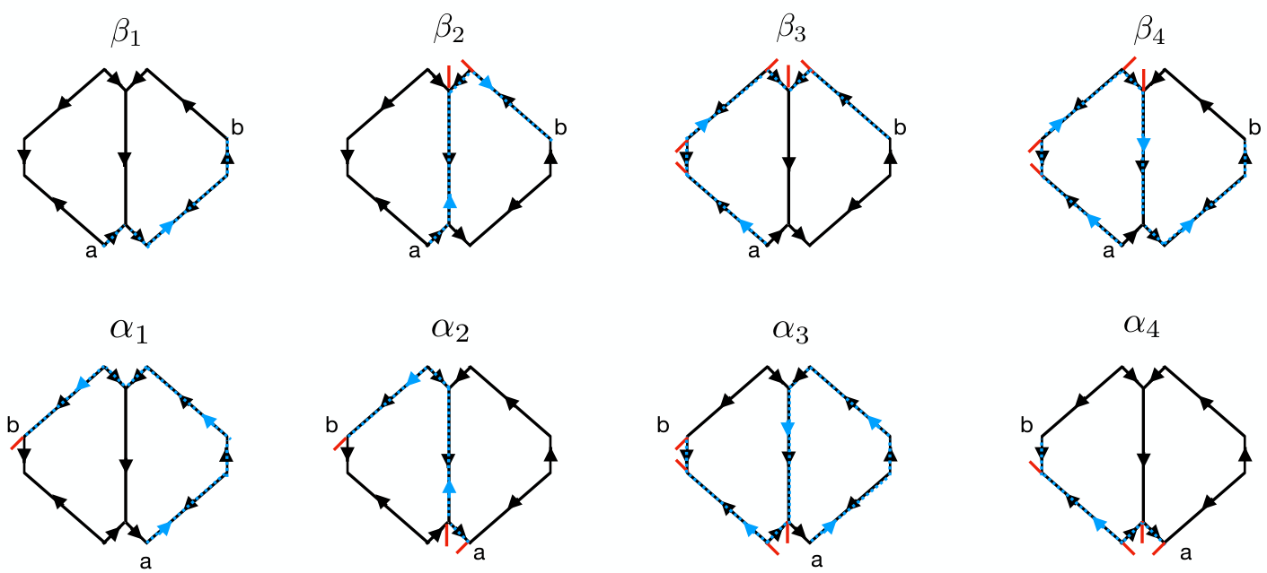
Let us fix a Kasteleyn orientation on the 2-manifold . Suppose we choose a closed oriented cycle on : namely is a set of edges in the hexagonalization of the ideal triangulation. Let be the number of the edges where the orientation along the path is opposed from the orientation determined by the Kasteleyn orientation. By we denote the number of left dimer sticks along the path , where the dimer stick is defined as the small continuation of all edges at the vertices of the hexagon. If we reach a dimer sticks along the a path on the left hand side of the path we call it a left dimer stick.
Let us explain this notation using Fig. 11. We start a blue path from point to point . We have four of the edges with orientations against the Kasteleyn orientation and therefore . Along the blue path we find the left dimer sticks (shown with red color) five times and therefore .
Let us define a sign associated with the closed path by
| (143) |
It turns out that this sign depends only on the spin structure (i.e. the equivalence class of the Kasteleyn orientations) and on the cohomology class of the path . The signs can thus be regarded as a map from a spin structure to an element of ((MR2410902, Theorem 1), see also (BB, Theorem 3.2.8)).
As an example, we consider the once-punctured torus. We have four equivalence classes of Kasteleyn orientations as in Fig. 4. Let us here discuss the case . To find we can draw the and -circle in the hexagonalization as in Fig. 12. We show four different representative paths for the cohomology class, both for the and the -cycle. The point is the starting point of the path and the red dimers are those dimers which are on the left side of the path . The result for different choice of path is the same, as long as they represent the same cohomology class in .
Appendix B Spin Mapping Class Group
In this appendix we study the number of spin structures kept fixed under a general element of the .
A general element of can be written as where are integers. Since and preserves the spin structure, for our purposes we can consider the integers modulo , so that we have elements of the form or . Moreover, since and preserves the spin structure, the discussion reduces to the following six cases (notice for example and act on the spin structures in the same way):
| (149) |
For each case, the action on the spin structure on each of the four spin structures can be worked out as
where those spin structures fixed under the mapping class group action are highlighted in red. This means that in general a mapping class group element preserves either one, two or four spin structures.
References
- (1) L. Chekhov and V. Fock, “Quantum Teichmuller space”, Theor. Math. Phys. 120, 1245 (1999), math/9908165.
- (2) R. M. Kashaev, “Quantization of Teichmueller spaces and the quantum dilogarithm”, Lett. Math. Phys. 43, 105 (1998).
- (3) J. Ellegaard Andersen and R. Kashaev, “A TQFT from Quantum Teichmüller Theory”, Commun. Math. Phys. 330, 887 (2014), arxiv:1109.6295.
- (4) J. Ellegaard Andersen and R. Kashaev, “A new formulation of the Teichmüller TQFT”, arxiv:1305.4291.
- (5) J. E. Andersen and R. Kashaev, “The Teichmüller TQFT”, arxiv:1811.06853, in: “International Congress of Mathematicians”, pp. 2527–2552.
- (6) R. Kashaev, “Quantum dilogarithm as a 6j symbol”, Mod. Phys. Lett. A 9, 3757 (1994), hep-th/9411147.
- (7) K. Hikami, “Hyperbolic structure arising from a knot invariant”, Internat. J. Modern Phys. A 16, 3309 (2001).
- (8) K. Hikami, “Asymptotics of the colored Jones polynomial and the A-polynomial”, Nucl. Phys. B 773, 184 (2007), math-ph/0407043.
- (9) T. Dimofte, S. Gukov, J. Lenells and D. Zagier, “Exact Results for Perturbative Chern-Simons Theory with Complex Gauge Group”, Commun. Num. Theor. Phys. 3, 363 (2009), arxiv:0903.2472.
- (10) T. Dimofte, “Quantum Riemann Surfaces in Chern-Simons Theory”, Adv. Theor. Math. Phys. 17, 479 (2013), arxiv:1102.4847.
- (11) T. D. Dimofte and S. Garoufalidis, “The Quantum content of the gluing equations”, Geom. Topol. 17, 1253 (2013), arxiv:1202.6268.
- (12) R. Kashaev, F. Luo and G. Vartanov, “A TQFT of Turaev–Viro Type on Shaped Triangulations”, Annales Henri Poincare 17, 1109 (2016), arxiv:1210.8393.
- (13) T. Dimofte, “Complex Chern-Simons Theory at Level k via the 3d–3d Correspondence”, Commun. Math. Phys. 339, 619 (2015), arxiv:1409.0857.
- (14) S. Garoufalidis and R. Kashaev, “Evaluation of state integrals at rational points”, Commun. Num. Theor. Phys. 09, 549 (2015), arxiv:1411.6062.
- (15) Y. Terashima and M. Yamazaki, “SL(2,R) Chern-Simons, Liouville, and Gauge Theory on Duality Walls”, JHEP 1108, 135 (2011), arxiv:1103.5748.
- (16) T. Dimofte, D. Gaiotto and S. Gukov, “Gauge Theories Labelled by Three-Manifolds”, Commun. Math. Phys. 325, 367 (2014), arxiv:1108.4389.
- (17) Y. Terashima and M. Yamazaki, “Semiclassical Analysis of the 3d/3d Relation”, Phys. Rev. D88, 026011 (2013), arxiv:1106.3066.
- (18) T. Dimofte and S. Gukov, “Chern-Simons Theory and S-duality”, JHEP 1305, 109 (2013), arxiv:1106.4550.
- (19) D. Gang, E. Koh and K. Lee, “Superconformal Index with Duality Domain Wall”, JHEP 1210, 187 (2012), arxiv:1205.0069.
- (20) D. Gang, N. Kim, M. Romo and M. Yamazaki, “Taming supersymmetric defects in 3d–3d correspondence”, J. Phys. A 49, 30LT02 (2016), arxiv:1510.03884.
- (21) D. Gang, N. Kim, M. Romo and M. Yamazaki, “Aspects of Defects in 3d-3d Correspondence”, JHEP 1610, 062 (2016), arxiv:1510.05011.
- (22) S. Chun, S. Gukov, S. Park and N. Sopenko, “3d-3d correspondence for mapping tori”, arxiv:1911.08456.
- (23) F. Bouschbacher, “Shear coordinates on the super-Teichmüller space”, https://tel.archives-ouvertes.fr/tel-00835500v1/document.
- (24) R. C. Penner and A. M. Zeitlin, “Decorated super-Teichmüller space”, J. Diff. Geom. 111, 527 (2019), arxiv:1509.06302.
- (25) N. Aghaei, M. Pawelkiewicz and J. Teschner, “Quantisation of super Teichmüller theory”, Commun. Math. Phys. 353, 597 (2017), arxiv:1512.02617.
- (26) N. Aghaei and M. Pawelkiewicz, “Heisenberg double and Drinfeld double of the quantum superplane”, arxiv:1909.04565.
- (27) I. C. H. Ip, R. C. Penner and A. M. Zeitlin, “ super-Teichmüller theory”, Adv. Math. 336, 409 (2018), arxiv:1605.08094.
- (28) I. C. Ip, R. C. Penner and A. M. Zeitlin, “On Ramond Decorations”, Commun. Math. Phys. 371, 145 (2019), arxiv:1709.06207.
- (29) C. Cremonini and P. Grassi, “Pictures from Super Chern-Simons Theory”, JHEP 2003, 043 (2020), arxiv:1907.07152.
- (30) V. Bouchard, P. Ciosmak, L. Hadasz, K. Osuga, B. Ruba and P. Suł kowski, “Super Quantum Airy Structures”, arxiv:1907.08913.
- (31) Y. Huang, R. C. Penner and A. M. Zeitlin, “Super McShane identity”, arxiv:1907.09978.
- (32) D. Stanford and E. Witten, “JT Gravity and the Ensembles of Random Matrix Theory”, arxiv:1907.03363.
- (33) P. Norbury, “Enumerative geometry via the moduli space of super Riemann surfaces”, arxiv:2005.04378.
- (34) D. Gang, “Chern-Simons Theory on Lens Spaces and Localization”, J. Korean Phys. Soc. 74, 1119 (2019), arxiv:0912.4664.
- (35) F. Benini, T. Nishioka and M. Yamazaki, “4d Index to 3d Index and 2d TQFT”, Phys. Rev. D86, 065015 (2012), arxiv:1109.0283.
- (36) M. Atiyah, “Topological quantum field theories”, Inst. Hautes Études Sci. Publ. D86, 175 (1988).
- (37) Y. Terashima and M. Yamazaki, “3d N=2 Theories from Cluster Algebras”, PTEP 2014, 023B01 (2014), arxiv:1301.5902.
- (38) L. Hodgkin, “Super Teichmüller spaces: punctures and elliptic points”, Lett. Math. Phys. 15, 159 (1988).
- (39) L. Crane and J. M. Rabin, “Super Riemann surfaces: uniformization and Teichmüller theory”, Comm. Math. Phys. 113, 601 (1988), http://projecteuclid.org/euclid.cmp/1104160351.
- (40) P. Bryant and L. Hodgkin, “Nielsen’s theorem and the super-Teichmüller space”, Ann. Inst. H. Poincaré Phys. T 58, 247 (1993).
- (41) Y. I. Manin, “Topics in noncommutative geometry”, Princeton University Press, Princeton, NJ (1991).
- (42) S. M. Natanzon, “Moduli of Riemann surfaces, real algebraic curves, and their superanalogs”, American Mathematical Society, Providence, RI (2004), Translated from the 2003 Russian edition by Sergei Lando.
- (43) P. W. Kasteleyn, “Dimer statistics and phase transitions”, J. Mathematical Phys. 4, 287 (1963).
- (44) D. Cimasoni and N. Reshetikhin, “Dimers on surface graphs and spin structures. I”, Comm. Math. Phys. 275, 187 (2007).
- (45) D. Cimasoni and N. Reshetikhin, “Dimers on surface graphs and spin structures. II”, Comm. Math. Phys. 281, 445 (2008).
- (46) D. Johnson, “Spin structures and quadratic forms on surfaces”, J. London Math. Soc. (2) 22, 365 (1980).
- (47) L. Dąbrowski and R. Percacci, “Spinors and diffeomorphisms”, Comm. Math. Phys. 106, 691 (1986), http://projecteuclid.org/euclid.cmp/1104115859.
- (48) T. Pantev and E. Sharpe, “Duality group actions on fermions”, JHEP 1611, 171 (2016), arxiv:1609.00011.
- (49) T. Fukuda and K. Hosomichi, “Super Liouville theory with boundary”, Nucl. Phys. B 635, 215 (2002), hep-th/0202032.
- (50) L. Hadasz, “On the fusion matrix of the N=1 Neveu-Schwarz blocks”, JHEP 0712, 071 (2007), arxiv:0707.3384.
- (51) L. Faddeev and A. Volkov, “Abelian current algebra and the Virasoro algebra on the lattice”, Phys. Lett. B 315, 311 (1993), hep-th/9307048.
- (52) L. Faddeev and R. Kashaev, “Quantum Dilogarithm”, Mod. Phys. Lett. A 9, 427 (1994), hep-th/9310070.
- (53) L. Faddeev, “Discrete Heisenberg-Weyl group and modular group”, Lett. Math. Phys. 34, 249 (1995), hep-th/9504111.
- (54) J.-P. Otal, “Le théorème d’hyperbolisation pour les variétés fibrées de dimension 3”, Astérisque 34, x (1996).
- (55) W. D. Neumann and D. Zagier, “Volumes of hyperbolic three-manifolds”, Topology 24, 307 (1985).
- (56) D. Cooper, M. Culler, H. Gillet, D. D. Long and P. B. Shalen, “Plane curves associated to character varieties of -manifolds”, Invent. Math. 118, 47 (1994).
- (57) J. Porti, “Torsion de Reidemeister pour les variétés hyperboliques”, C. R. Acad. Sci. Paris Sér. I Math. 320, 59 (1995).
- (58) E. Witten, “Quantum Field Theory and the Jones Polynomial”, Commun. Math. Phys. 121, 351 (1989).
- (59) V. Mikhaylov, “Analytic Torsion, 3d Mirror Symmetry And Supergroup Chern-Simons Theories”, arxiv:1505.03130.
- (60) M. Culler, N. M. Dunfield and J. R. Weeks, “SnapPy, a computer program for studying the geometry and topology of 3-manifolds”, http://snappy.computop.org.
- (61) V. Mikhaylov, “Teichmüller TQFT vs. Chern-Simons theory”, JHEP 1804, 085 (2018), arxiv:1710.04354.
- (62) V. Mikhaylov and E. Witten, “Branes And Supergroups”, Commun. Math. Phys. 340, 699 (2015), arxiv:1410.1175.
- (63) R. B. Zhang, “Finite-dimensional representations of and its connection with quantum ”, Lett. Math. Phys. 25, 317 (1992).
- (64) S. Clark, “Odd knot invariants from quantum covering groups”, Algebr. Geom. Topol. 17, 2961 (2017).
- (65) A. Kapustin and E. Witten, “Electric-Magnetic Duality And The Geometric Langlands Program”, Commun. Num. Theor. Phys. 1, 1 (2007), hep-th/0604151.
- (66) Q. Chen and T. Yang, “Volume conjectures for the Reshetikhin-Turaev and the Turaev-Viro invariants”, arxiv:1503.02547.
- (67) D. Gang, M. Romo and M. Yamazaki, “All-Order Volume Conjecture for Closed 3-Manifolds from Complex Chern–Simons Theory”, Commun. Math. Phys. 359, 915 (2018), arxiv:1704.00918.
- (68) E. Witten, “Analytic Continuation Of Chern-Simons Theory”, AMS/IP Stud. Adv. Math. 50, 347 (2011), arxiv:1001.2933.
- (69) C. Cordova and D. L. Jafferis, “Toda Theory From Six Dimensions”, JHEP 1712, 106 (2017), arxiv:1605.03997.
- (70) J. Yagi, “3d TQFT from 6d SCFT”, JHEP 1308, 017 (2013), arxiv:1305.0291.
- (71) S. Lee and M. Yamazaki, “3d Chern-Simons Theory from M5-branes”, JHEP 1312, 035 (2013), arxiv:1305.2429.
- (72) C. Cordova and D. L. Jafferis, “Complex Chern-Simons from M5-branes on the Squashed Three-Sphere”, JHEP 1711, 119 (2017), arxiv:1305.2891.
- (73) H. L. Verlinde, “Conformal Field Theory, 2- Quantum Gravity and Quantization of Teichmuller Space”, Nucl. Phys. B337, 652 (1990).
- (74) J. Teschner, “From Liouville theory to the quantum geometry of Riemann surfaces”, hep-th/0308031, in: “Mathematical physics. Proceedings, 14th International Congress, ICMP 2003, Lisbon, Portugal, July 28-August 2, 2003”.
- (75) J. Teschner, “An Analog of a modular functor from quantized teichmuller theory”, math/0510174.
- (76) J. Teschner, “Quantization of the Hitchin moduli spaces, Liouville theory, and the geometric Langlands correspondence I”, Adv. Theor. Math. Phys. 15, 471 (2011), arxiv:1005.2846.
- (77) L. Faddeev, R. Kashaev and A. Volkov, “Strongly coupled quantum discrete Liouville theory. 1. Algebraic approach and duality”, Commun. Math. Phys. 219, 199 (2001), hep-th/0006156.
- (78) L. Faddeev and R. Kashaev, “Strongly coupled quantum discrete Liouville theory. 2. Geometric interpretation of the evolution operator”, J. Phys. A 35, 4043 (2002), hep-th/0201049.
- (79) L. F. Alday, D. Gaiotto and Y. Tachikawa, “Liouville Correlation Functions from Four-dimensional Gauge Theories”, Lett. Math. Phys. 91, 167 (2010), arxiv:0906.3219.
- (80) V. Belavin and B. Feigin, “Super Liouville conformal blocks from N=2 SU(2) quiver gauge theories”, JHEP 1107, 079 (2011), arxiv:1105.5800.
- (81) G. Bonelli, K. Maruyoshi and A. Tanzini, “Instantons on ALE spaces and Super Liouville Conformal Field Theories”, JHEP 1108, 056 (2011), arxiv:1106.2505.
- (82) G. Bonelli, K. Maruyoshi and A. Tanzini, “Gauge Theories on ALE Space and Super Liouville Correlation Functions”, Lett. Math. Phys. 101, 103 (2012), arxiv:1107.4609.
- (83) V. Pestun, “Localization of gauge theory on a four-sphere and supersymmetric Wilson loops”, Commun. Math. Phys. 313, 71 (2012), arxiv:0712.2824.
- (84) N. Hama and K. Hosomichi, “Seiberg-Witten Theories on Ellipsoids”, JHEP 1209, 033 (2012), arxiv:1206.6359, [Addendum: JHEP 10, 051 (2012)].
- (85) R. Benedetti and C. Petronio, “Spin structures on 3-manifolds via arbitrary triangulations”, Algebr. Geom. Topol. 14, 1005 (2014).
- (86) R. Budney, “Combinatorial spin structures on triangulated manifolds”, Algebr. Geom. Topol. 18, 1259 (2018).
- (87) D. Gaiotto and A. Kapustin, “Spin TQFTs and fermionic phases of matter”, Int. J. Mod. Phys. A31, 1645044 (2016), arxiv:1505.05856, in: “Proceedings, Gribov-85 Memorial Workshop on Theoretical Physics of XXI Century: Chernogolovka, Russia, June 7-20, 2015”, pp. 1645044.
- (88) P. C. Argyres, A. LeClair and S. Tye, “On the possibility of fractional superstrings”, Phys. Lett. B 253, 306 (1991).
- (89) A. LeClair, D. Nemeschansky and N. Warner, “S matrices for perturbed N=2 superconformal field theory from quantum groups”, Nucl. Phys. B 390, 653 (1993), hep-th/9206041.
- (90) A. Belavin, V. Belavin and M. Bershtein, “Instantons and 2d Superconformal field theory”, JHEP 1109, 117 (2011), arxiv:1106.4001.
- (91) T. Nishioka and Y. Tachikawa, “Central charges of para-Liouville and Toda theories from M-5-branes”, Phys. Rev. D84, 046009 (2011), arxiv:1106.1172.
- (92) I. C.-H. Ip and M. Yamazaki, “Quantum Dilogarithm Identities at Root of Unity”, Int. Math. Res. Not. 2016, 669 (2016), arxiv:1412.5777.
- (93) I. Coman, M. Gabella and J. Teschner, “Line operators in theories of class , quantized moduli space of flat connections, and Toda field theory”, JHEP 1510, 143 (2015), arxiv:1505.05898.
- (94) E. Frenkel, S. Gukov and J. Teschner, “Surface Operators and Separation of Variables”, JHEP 1601, 179 (2016), arxiv:1506.07508.
- (95) M. Blau and G. Thompson, “Derivation of the Verlinde formula from Chern-Simons theory and the G/G model”, Nucl. Phys. B 408, 345 (1993), hep-th/9305010.
- (96) D. Montano, K. Aoki and J. Sonnenschein, “Topological Supergravity in Two-dimensions”, Phys. Lett. B 247, 64 (1990).
- (97) A. H. Chamseddine, “Superstrings in arbitrary dimensions”, Phys. Lett. B 258, 97 (1991).
- (98) D. Cangemi and M. Leblanc, “Two-dimensional gauge theoretic supergravities”, Nucl. Phys. B 420, 363 (1994), hep-th/9307160.
- (99) C. Teitelboim, “Gravitation and Hamiltonian Structure in Two Space-Time Dimensions”, Phys. Lett. B 126, 41 (1983).
- (100) R. Jackiw, “Lower Dimensional Gravity”, Nucl. Phys. B 252, 343 (1985).