A unifying framework for the analysis of projection-free first-order methods under a sufficient slope condition
Abstract
The analysis of projection-free first order methods is often complicated by the presence of different kinds of "good" and "bad" steps. In this article, we propose a unifying framework for projection-free methods, aiming to simplify the converge analysis by getting rid of such a distinction between steps. The main tool employed in our framework is the Short Step Chain (SSC) procedure, which skips gradient computations in consecutive short steps until proper stopping conditions are satisfied. This technique allows us to give a unified analysis and converge rates in the general smooth non convex setting, as well as convergence rates under a Kurdyka-Łojasiewicz (KL) property, a setting that, to our knowledge, has not been analyzed before for the projection-free methods under study. In this context, we prove local convergence rates comparable to those of projected gradient methods under the same conditions.
Our analysis relies on a sufficient slope condition, ensuring that the directions selected by the methods have the steepest slope possible up to a constant among feasible directions. This condition is satisfied, among others, by several Frank-Wolfe (FW) variants on polytopes, and by some projection-free methods on convex sets with smooth boundary.
Keywords: Nonconvex optimization,
First-order optimization, Projection-free optimization, Frank-Wolfe variants, Kurdyka-Łojasiewicz inequality.
AMS subject classification: 46N10, 65K05, 90C06, 90C25, 90C30
1 Introduction
Projection-free first-order methods aim to provide a valid alternative to projected gradient approaches for the constrained optimization of a smooth objective , in settings where projecting on the feasible set may be unpractical. Popular methods of this kind are the FW algorithm [17] and its variants (see, e.g., [18], [30] and references therein), which have many applications in sparse and structured optimization (see, e.g., [18], [22], [24], [39] and references therein).
In this paper, we present a specific algorithmic framework that can easily embed
a number of projection-free (deterministic) methods proposed in the literature. This enables us to give a unified theoretical analysis for the methods at hand and new convergence results in the non convex case. More specifically, the framework we propose aims to overcome an annoying issue affecting the analysis of projection-free methods, that is the presence of "bad iterations", i.e., iterations where we cannot show good progress. This happens when we are forced to take a short step along the search direction to guarantee feasibility of the iterate. The number of short steps typically needs to be upper bounded in the convergence analysis with "ad hoc" arguments (see, e.g., [18] and [30]). The main idea behind our method is to chain several short steps by skipping gradient updates until proper stopping conditions are met. This has the additional benefit to rule out unpractical convergence rates due to large numbers of short steps in the analysis of the methods, like, for instance, in the PFW algorithm on the dimensional simplex, where the best known upper bound on the number of consecutive short steps is [30].
The projection-free first order methods we consider satisfy a sufficient slope condition related to the slope along descent directions. Essentialy, for any direction selected by the method in and any direction feasible in we must have
for a fixed (independent from and ). Thus any direction selected by the method must be, up to a fixed constant, the steepest descent direction among feasible directions. The sufficient slope condition rules out the well known zig zagging behaviour of the classic FW method, whose directions can be almost orthogonal to the gradient on the interior of the feasible domain, leading to a slow convergence of even for smooth strongly convex objectives [14, 17, 30, 43]. We show that this condition applies to the AFW, the PFW and the FW method with in face directions (FDFW) (see, e.g., [18] and [20]) on polytopes, to a retraction based approach on convex sets with smooth boundary as the one proposed in [33], to the FDFW method on sublevel sets of smooth strongly convex functions, and to tailored approaches over product domains.
We analyze convergence rates for non convex smooth objectives both in the general case and under the Kurdyka-Łojasiewicz property ([3], [8], [9]; see also Section 8.2 for a review of the essential definitions). This property holds for semialgebraic functions and more in general for functions definable in an -minimal class (see, e.g., [3], [8]). While there are many works on the convergence rates of proximal subgradient type methods under KL properties (see, e.g., [3], [4], [10], [42], [44]), we are not aware of previous analyses including projection-free methods for convex sets and smooth non convex objectives. In the convex setting, FW variants have been analyzed on polytopes [28] and uniformly convex sets (see, e.g., [29], [45]) under Hölderian error bound conditions, to interpolate between the well known rate for general convex objectives and the faster rates for strongly convex ones proved in [19] and [30]. These Hölderian error bound conditions are equivalent to certain KL properties for convex objectives, as proved for a more general class of error bounds in [10]. As for the smooth non convex case, in [35] a KL property leading to linear convergence of some methods using retractions is proved for a quadratic problem on the Stiefel manifold; in [7] the convergence of a method using orthographic retractions is analyzed on proximally smooth surfaces under a KL property (see also Remark 8.2).
When dealing with the FW method and its variants, which represent a specific class of projection-free first-order methods, the SSC procedure has the additional advantage that it skips the computation of the solutions of linear programming subproblems. Different approaches to avoid computations of those solutions have been discussed in [12] , [11] for convex optimization over polytopes. The blended conditional gradient introduced in [12] uses projections on the convex hull of the current active set as an alternative to pairwise or away FW steps, but its analysis still allows for short steps. Other works in projection-free optimization (e.g. [21], [32]) rely on the classic FW method to approximately compute the projection in accelerated projected gradient methods for convex objectives. To our knowledge this approach, called conditional gradient sliding, has not yet been combined effectively with faster FW variants, and it does not currently lead to any improvement on the linear oracle complexity of the FW method. Our methods using the SSC procedure instead have a complexity of both in gradients and linear oracles for non convex objectives satisfying a KL property implied e.g. by the Luo Tseng error bound [36] under some mild separability conditions for the stationary points [34, Theorem 4.1]. This error bound is known to hold in a variety of convex and non convex settings (see references in [34]).
The structure of the paper is as follows. In Section 2, we define some notation and state some preliminary results from convex analysis. In Section 3, we introduce a sufficient slope property for first-order projection free methods. We define the SSC procedure in Section 4, and prove it can be applied to generate some subgradient descent-like sequences (see, e.g., [4], [10], [36]) adapted to our particular setting. In Section 5, we state the main convergence results. In Section 6, we show examples of methods fitting our framework. Finally, some proofs, technical lemmas and background material can be found in the appendix.
2 Notation and preliminaries
We consider the following constrained optimization problem:
| (2.1) |
In the rest of the article is a compact and convex set, unless specified otherwise, and with -Lipschitz gradient:
We define as the diameter of , for and for . For sequences we write instead of when is clear from the context, with by default and . Given a function with values in we use the notation
for and we use the same notation for non strict inequalities.
For subsets of we define as
as the neighborhood of of radius and in particular as the open euclidean ball of radius and center . When is closed and convex we define as the projection on . If is a cone then we denote with its polar.
We now state some elementary properties related to the tangent and the normal cones, where for we denote with and the tangent and the normal cone to in respectively. The next proposition (from [41], Theorem 6.9) characterizes these cones for closed convex subsets of .
Proposition 2.1.
Let be a closed convex set. For every point we have
| int | |||
We have the following formula connecting the maximal "slope" of a linear function along feasible directions to the tangent and the normal cone:
Proposition 2.2.
If is a closed convex subset of , then for every
This property is a consequence of the Moreau-Yosida decomposition [41] and we refer the reader to Section 8.1 in the Appendix for a detailed proof. In the rest of the article to simplify notations we often use as a shorthand for , so that by Proposition 2.2 first order stationarity conditions in for the gradient become equivalent to .
3 Sufficient slope condition
Let be a first-order optimization method defined for smooth functions on a closed subset of . We assume that given first-order information the method always selects along a feasible descent direction, so that for we can define
as the possible descent directions selected by when , for some (see Algorithm 1). When is first-order stationary, we set , otherwise we always assume .
| Initialization. , . |
| 1. If is stationary, then STOP |
| 2. select a descent direction |
| 3. set for some stepsize |
| 4. set , go to Step 1. |
We want to formulate a "sufficient slope" condition for the descent directions selected by with respect to the steepest slope among feasible directions. In order to do that, we define the directional slope lower bound as
if . Otherwise by our assumptions is stationary for , and we set . With these definitions for any ,
| (3.1) |
since if then for any feasible descent direction by Proposition 2.2, and if by definition . Given a subset of we can finally define the slope lower bound
where in the second equality we used that (3.1) holds with equality if . For simplicity if we write instead of .
In Section 6, we show a few examples of methods and sets satisfying a sufficient slope condition, i.e., cases where the slope lower bound is strictly grater than zero.
4 First order projection free methods with SSC procedure
In this section, we briefly recall the subgradient descent sequence conditions used in the analysis of a variety of descent methods (see, e.g., [4], [10], [36]), with a few simple adaptations to our smooth constrained projection-free setting. We then introduce the SSC procedure, and show how it allows us to obtain our adapted subgradient descent sequences.
4.1 Subgradient descent sequences for projection-free methods
Let be a proper lower semicontinuous function and let be its limiting subdifferential. We refer the reader to Section 8.2 of the appendix for a brief reivew of the Fréchet subdifferential and the related KL property as defined in [3], [4]. In this work we are only interested in the case with the indicator function for . We anyway notice that the abstract convergence result we give in Section 5 holds for general lower semicontinuous functions.
Subgradient descent sequences as defined in [10] satisfy the following properties for some given :
| (H1) | ||||
| (H2) | ||||
Since is closed, condition (H2) is true iff and
| (4.2) |
In our smooth constrained setting, that is when , by (8.8) we can rewrite (4.2) as
| (4.3) |
However, for projection-free methods equation (4.2) and in particular (4.3) do not hold in general, even in linear convergence settings.

boundary of a sphere.

near the boundary of a polytope.
Intuitively, for these methods the first obstacle for condition (4.3) or variants is that if and with we have, for typical choices of the stepsize (see figure 1(a)):
This leads us to introduce the weaker condition
| (H’2) |
for some auxiliary point s.t. and
| (4.4) |
In particular in the setting of figure 1(a) a typical choice is , as we shall see more formally in the next section. In the rest of this article (H’2) always comes with (4.4) for .
As anticipated, condition (H’2) is weaker than (H2) if one is already assuming (H1). Indeed if (H1) and (H2) hold then
where the second inequality directly follows from (H2) in the form (4.2). One can then satisfy (H’2) and (4.4) by taking .
In our setting, that is when , we use the smooth version of (H’2):
| (H’2a) |
with analogous conditions on .
4.2 The SSC procedure
The second (and arguably most important) issue for applying conditions such as (4.3) to projection-free methods is the presence of short steps. Given a projection-free first-order method , we say that the step is short if the stepsize is maximal, that is . Roughly speaking, when is close enough to and points toward we have (see figure 1(b) with )
An analogous issue affects also weaker variants of (4.3), including (H’2a). In order to address this issue, we apply the SSC procedure to first order methods (Algorithm 2). This procedure (Algorithm 3) chains consecutive short steps, skipping updates for the gradient and possibly for related information, like linear minimizers, until proper stopping conditions are met. After the SSC returns a candidate point , the method may still choose another point in Step 4, selecting a with a smaller objective value than and satisfying (H1):
| (4.5) |
The method can always take , since, as we prove later in this section, the following inequality holds
| Initialization. , . |
| 1. while is not stationary: |
| 2. |
| 3. |
| 4. select satisfying (4.5) |
| 5. . |
| Initialization. , . |
| Phase I |
| 1. select , |
| 2. if then: |
| 3. return |
| Phase II |
| 4. compute with (4.7) |
| 5. let |
| 6. if then: |
| 7. return |
| Phase III |
| 8. |
| 9. if then: |
| 10. return |
| 11. , go to Step 1. |
Given that the gradient is constant during the SSC, this procedure can be viewed as an application of for the minimization of the linearized objective with peculiar stepsizes and stopping criterion. Fundamentally, these must ensure that the linearized objective is still a sufficiently accurate approximation of on the generated sequence, and that the directions selected are descent directions not only for but also for the true objective .
We can split the SSC into three phases. First, the SSC computes a feasible descent direction if it exists, otherwise and the algorithm returns . Notice that iff is stationary w.r.t. the approximated gradient . Second, the stepsize is computed by taking the minimum between the maximal stepsize and an auxiliary stepsize . The maximal stepsize may depend on boundary conditions but also on additional information available like the active set in the AFW and in the PFW. In the theoretical analysis, we only need to assume termination of the procedure and . In particular, in Phase II iff , or equivalently if is not feasible from for the auxiliary set (see (4.6)). As we shall see later in this section, when we always have , and therefore Phase II can never return (which could cause an infinite loop in Algorithm 2). In the third and final phase, the new point of the SSC is computed. Then the procedure terminates if , otherwise it continues without updating the gradient.
We now define the auxiliary step size , which allows us to retrieve the descent sequence conditions (H1) and (H’2a). Let
| (4.6) |
We define
| (4.7) |
where is the maximal feasible stepsize in the direction starting from with respect to . Since is the intersection of two balls there is a simple closed form expression for . Given that it is immediate to check that if
which corresponds to the constant stepsize for gradient descent (when ), and where since is by assumption a descent direction for .
The second ball appearing in the definition of does not depend on and can be rewritten as
| (4.8) |
Then for any we have
| (4.9) |
where the first inequality is the standard descent lemma and the second follows from (4.8). Let now . Since , and if then by definition of , by induction we obtain for every . Therefore thanks to (4.9) for every we have the sufficient decrease condition
| (4.10) |
We now show how the condition guarantees that the true objective is monotone decreasing during the SSC.
Lemma 4.1.
Assume . Then for every we have
and thus in particular .
Proof.
We have
where we used and the Lipschitzianity of in the first inequality and
in the second. ∎
We can now prove the descent sequence conditions (H1) and (H’2a) for a sequence generated by Algorithm 2.
Proposition 4.1.
Proof.
Let and let be such that .
Inequality (4.10) applied with gives (4.11). Moreover, by taking for some the conditions
| (4.13) |
are satisfied by Lemma 4.1 and (4.10).
Let now and . We have
| (4.14) | ||||
where we used the 1-Lipschitzianity of the projections on convex sets in the first inequality. We now distinguish four cases according to how the SSC terminates.
Case 1: or . Since there are no descent directions must be stationary for the gradient . Equivalently, . We can now write
where we used (4.14) in the first inequality and in the equality. We now prove that if then necessarily . This is clear if is stationary for . Otherwise is a feasible descent direction, so that and also . But then and the SSC can’t terminate in Phase I or Phase II, in contradiction with .
Before examining the remaining cases we remark that if the SSC terminates in Phase III then must be maximal w.r.t. the conditions or , which imply (case 3) and (case 4) respectively. On the other hand if then necessarily . In this case we cannot have , otherwise the SSC would terminate in Phase III of the previous cycle. Therefore necessarily (Case 2).
Case 2: . We can rewrite the condition as
| (4.15) |
Thus
| (4.16) |
where the first inequality follows from (4.14), the second from , and the third from (4.15). Then satisfies the desired conditions.
Case 3: and . Then from it follows
| (4.17) |
and implies
| (4.18) |
Combining (4.17) with (4.18) we obtain
| (4.19) |
Thus
where we used (4.18), (4.19) in the last inequality and the rest follows reasoning as for (4.16). In particular we can take .
Case 4: and .
By the characterization of in (4.8) the condition can be rewritten as
| (4.20) |
For every we have
| (4.21) |
We now want to prove that for every
| (4.22) |
Indeed, we have
where we used (4.20) in the first equality, (4.21) in the second, for every in the first inequality and in the second inequality.
We also have
| (4.23) | ||||
Thus for
| (4.24) |
where we used (4.23) in the first inequality and (4.20) in the second.
We finally have
where we used (4.22), (4.24) in the last inequality and the rest follows reasoning as for (4.16). In particular satisfies the desired properties.
It remains to prove that satisfies (H1) and (H’2a). The first condition (H1) clearly holds by (4.5). As for (H’2a), we have
where the first inequality follows from (4.5), the second from (4.11), and the third from (4.12). Finally, since , by (4.13) the conditions (4.4) on are satisfied. ∎
As an immediate corollary we have convergence to the set of stationary points with a rate of for the norm of the projected gradient . While the norm of the projected gradient may not be available, by (4.11) we have the readily available upper bound , which has an analogous convergence rate.
Corollary 4.1.
Proof.
The sequence is decreasing by (4.5) and (4.11) . Thus by compactness and in particular . Since we also have and by (4.11) . Let be any convergent subsequence of . For chosen as in the proof of Proposition 4.1 we have because in case 1 and case 2, by (4.19) in case 3, and by (4.22) in case 4. Therefore
Furthermore, again by Proposition 4.1, so that with . Then and is stationary.
Remark 4.1.
The proof of Proposition gives an easy way to retrieve . In particular it shows that one can take with in case 1 and case 2, in case 3 and
in case 4.
Remark 4.2.
For any we have
where the first inequality follows from Proposition 2.2 and the second by the assumption on . Therefore at the price of computing and a related descent directions we have upper and lower bounds separated by a factor of for .
5 Convergence properties
In this section, we use the descent sequence properties proved in the previous section in combination with a KL property for smooth functions to obtain convergence rates with respect to the objectives and the tail length of the iterate sequence. First, we give an abstract convergence lemma for proper lower semicontinuous functions. We then apply this lemma in combination with Proposition 4.1 to prove convergence rates for Algorithm 2 under finite termination of the SSC, and thus in particular for the examples discussed in Section 6.
For the abstract lemma with respect to the foundational work [4] we only have the weaker condition (H’2) instead of (H2), where the proof of the convergence lemma [4, Lemma 2.6] relies on the stronger condition. We therefore present a different proof technique in Section 8.3 of the appendix based on Karamata’s inequality ([25], [27]).
Before stating the main convergence result we need to introduce a one dimensional worst case sequence related to the desingularizing function , which we use bound the error on the objective. With respect to the (different) worst case sequence introduced in [10] we do not require neither the moderate behavior hypothesis on nor to be Lipschitz regular.
Let be a continuous monotone non increasing function finite in . For we define
with the convention . Since is continuous and strictly increasing if
is non empty then it has a maximum and
| (5.1) |
Otherwise
| (5.2) |
Let be equal to applied times, with the convention . Then the worst sequence related to an initial error is . Given that by continuity is upper bounded in every interval with , we have the limit
| (5.3) |
for every .
We can now state the main convergence result for proper lower semicontinuous functions.
Proposition 5.1.
Condition (5.6) is a slight refinement of [4, condition (4)]. It implies of course , and the additional terms on the LHS are sufficient to ensure . It is not difficult to see from the proofs that it can be replaced with . When the desingularizing function is of the form with we obtain more explicit convergence rates on the length and the objective gap. For convex functions this KL property is equivalent to Hölderian error bounds, as proved more in general in [10, Theorem 5].
Corollary 5.1.
Under the assumptions of Proposition 5.1, let for some . Then
| (5.9) |
Moreover
| (5.10) |
Finally, the implicit constants can be taken as functions of , and in particular independent from .
As a corollary of Proposition 5.1, by Proposition 4.1 we have the following results on the convergence rates of Algorithm 2:
Corollary 5.2.
Let us consider Problem (2.1) with satisfying the KL inequality w.r.t. in . Assume that is generated by Algorithm 2, and that the method in the SSC satisfies the following conditions:
- •
the SSC procedure always terminates in a finite number of steps;
- •
.
Assume that (5.4), (5.5) and (5.6) hold with and . Then the sequence converges to a stationary point and the convergence rates (5.7) and (5.8) hold.
Proof.
6 Analysis of some projection-free first-order methods
Here, we report some relevant examples of projection-free first-order methods and show that those methods satisfy the assumptions given in Corollary 5.2. More specifically, we show finiteness of the SSC procedure and that a sufficient slope condition is satisfied when the method is applied over a specific class of feasible sets. The reported examples include the AFW, PFW, FDFW on polytopes, the FDFW on sublevel sets of strongly convex smooth functions, a method based on orthographic retractions for convex sets with smooth boundary, as well as combination of these methods on product domains. At the end of the section we show how to apply our framework together with a KL property of (non convex) quadratic programming problems to obtain an asymptotic linear convergence rate for some FW variants.
Before giving the examples we prove a broad SSC finite termination criterion, showing that the procedure ends when using a first order method with mild convergence properties for linear objectives.
Lemma 6.1.
Assume that the method applied to any linear function and with every stepsize maximal always generates a (possibly finite) sequence such that
| (6.1) |
Then the SSC with the method always terminates in a finite number of steps.
Proof.
Assume by contradiction that the SSC generates an infinite sequence . In this case the method applied in the SSC with gradient always does maximal steps, since the SSC terminates as soon as so that . Let . Then by (6.1) we can take subsequence of indexes such that . We claim that , in contradiction with the strict monotonicity of . Indeed we have
by definition of in the first inequality and by Proposition 2.2 in the second. ∎
6.1 PFW, AFW, FDFW directions
The AFW and PFW depend from a set of "elementary atoms" such that . Given , for a base point we can define
the family of possible active sets for . In the rest of the article is always clear from the context and for simplicity we write PFW, AFW instead of , . For , , is a PFW direction with respect to the active set and gradient iff
Similarly, given , , is an AFW direction with respect to the active set and gradient iff
| (6.2) |
where is a classic Frank Wolfe direction
| (6.3) |
If the FW method is applied to a linear objective it clearly terminates after at most one maximal step, with . As for the AFW or the PFW, they generate a sequence of active sets with proper convex combination of the elements in . After a FW step or a PFW step the linear minimizer is always in the active set, and we assume that no other point can be added at the step . In particular, . Now on the one hand, all the linear minimizers added to the active set can’t be dropped from the active set, since the gradient doesn’t change. On the other hand, after every maximal away or PFW step the element corresponding to the away direction is dropped from the active set. Furthermore, as the FW method also the AFW terminates after a maximal FW step. Then the AFW and the PFW applied to linear objectives terminate in at most steps. Applying Lemma 6.1 to obtain finite SSC termination we have the following:
Proposition 6.1.
For the FW, the PFW and the AFW applied to a linear objective the number of maximal steps is bounded, provided that no points beside linear minimizers are added to the active set. In particular, under this assumption for these methods the SSC terminates.
The FDFW from [18] relies only on the current point and the current gradient to choose a descent direction and, unlike the AFW and the PFW, does not need to keep track of the active set. This method makes use of a linear minimization oracle
for varying among the faces of . Let be the minimal face of containing . The in face direction is defined as
The selection criterion is then analogous to the one used by the AFW:
| (6.4) |
For the FDFW we assume that the maximal stepsize is given by feasibility conditions as in [18]:
| (6.5) |
Then after a maximal in face step from we have because lies on the boundary of . Whence there can only be a finite number of consecutive such steps. Furthermore, we’ve seen that after a maximal FW step every method applied to a linear objective terminates. Applying Lemma 6.1 to obtain finite SSC termination we have the following:
Proposition 6.2.
The FDFW on any compact and convex set does at most consecutive maximal steps. In particular, for this method the SSC terminates.
We write instead of in the rest of the paper.
When is a polytope and the sufficient slope conditions hold for the directions we introduced. Before stating a lower bound for in this setting we need to recall the definition of pyramidal width as it was given in [30]. We refer the reader to [40] for a discussion of various properties of this parameter.
For a given the pyramidal directional width is defined as
| (6.6) |
and the pyramidal width is defined as
Here we use one key property of which relates it to the slope along the PFW direction. We have the following lower bound (see [30, equation (12)])
| (6.7) |
where is any direction in which is also a descent direction11 1 In [30] the direction is defined as a possible error direction , where is an optimal point of a convex objective with . However, this definition is equivalent to ours. Indeed if then by convexity it must be a feasible descent direction for . Conversely, every feasible descent direction is always an error direction as defined above for some choice of , i.e. consider with positive definite such that . for . Another relevant property is that by (6.6) we have that is monotone decreasing in , so that if is the set of vertexes of we always have .
Proposition 6.3.
Let . Then
| (6.8) | ||||
Proof.
Let be such that . Then there exists descent directions for feasible for from , and
so that
| (6.9) |
where we used Proposition 2.2 in the last equality. Thanks to (6.9) taking the min on all the feasible descent directions in the LHS of (6.7) we obtain
We now have
and the first part of (6.8) follows by taking the inf on the LHS for and such that . Inequality (6.8) for the AFW method is a corollary since
as it follows immediately from the definitions (see also [30, equation (6)]).
For the FDFW, first observe that for any :
| (6.10) | ||||
where we used in the inequality and the last equality follows immediately from the definition of . We then have
| (6.11) |
where the first inequality follows from the choice criterion (6.4) together with , we used (6.10) in the second inequality, and (6.7) in the third. The thesis follows by taking the inf on and in the LHS and the sup on in the RHS. ∎
6.2 FW and FDFW on sublevel sets of strongly convex smooth functions
In spite of the zig-zagging behaviour discussed in the introduction, in any fixed point of a polytope the FW directions do satisfy the sufficient slope condition, e.g. by Proposition 6.3 since they are selected by the AFW and the PFW when the active set is a singleton. This property can be extended (uniformly) to the boundaries of sublevel sets of smooth strongly convex functions. As a consequence, using that the FDFW selects FW directions on the boundary of strictly convex sets, we also obtain a global slope bound for this method.
Proposition 6.4.
Let be -strongly convex and with -Lipschitz gradient, , . Then:
| (6.12) | |||
| (6.13) |
Proof.
Since for every
we can apply Lemma 8.1 with . We obtain
| (6.14) |
First, by -smoothness we have:
| (6.15) |
Second, by strong convexity
| (6.16) |
where we used in the equality. The first part of the thesis follows applying (6.15) and (6.16) to the RHS of (6.14).
By strong convexity for every
and therefore . This clearly implies
| (6.17) |
Analogously, by smoothness for every
| (6.18) |
and therefore . We can now give a slope bound for :
| (6.19) | ||||
where we used (6.11) in the first inequality, in the first equality, (6.17) in the second inequality, by (6.18) in the third inequality, and in the last one. But on the boundary the FDFW selects FW directions so that (6.12) holds also for the FDFW, and in particular (6.13) follows by combining (6.12) with (6.19) for points on the interior.
∎
Remark 6.1.
The slope bound (6.13) clearly holds for any method selecting FW directions on the boundary and other directions on the interior satisfying the sufficient slope condition for (e.g. the negative gradient).
6.3 Orthographic retractions for convex sets with smooth boundary
In this section we show an example of how the SSC can be employed effectively to deal with short steps also in non linearly constrained settings. More specifically, we consider here the case of compact, convex, full dimensional and with smooth boundary of class (e.g., the unitary ball w.r.t. , with . In this case for we can define as the outward pointing normal and as the tangent hyperplane to in . For , , we then define as the first intersection between and . By smoothness is always defined for small enough. This transformation is called an orthographic retraction, and can be easily extended to manifolds with arbitrary codimension. Orthographic retractions are widely used in manifold optimization for manifolds of class at least (see e.g. [1], [2], [26], [46]), in which case it can be proved that they are differentiable retractions [1]. In the codimension 1 case orthographic retractions were used in [7] for optimization over proximally smooth surfaces, and in [33] for optimization on sublevel sets of convex functions with Lipschitz gradient. In these works the additional regularity assumptions ensure that the manifold is sufficiently flat so that steps with length proportional to are effective. Here we do not need additional regularity assumptions, thanks to the SSC which allows our method to choose shorter steps while skipping gradient computations.
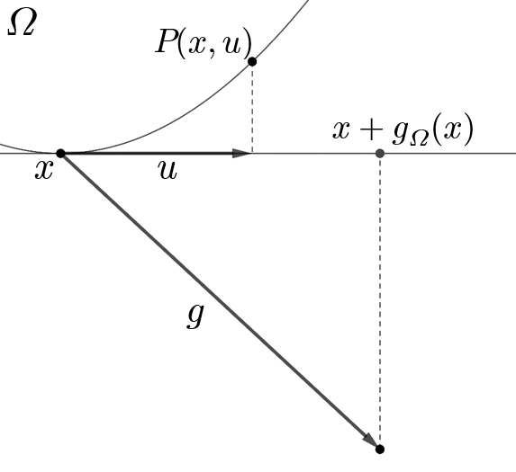
from .

For we denote with and the components of along and , so that , with . We can finally define the Short Orthographic Retractions (SOR) method directions simply as if , and using orthographic projections when is in
More precisely, in this case we define
where is a proper "shrinking coefficient", ensuring that the orthographic projection is taken close to enough to satisfy the usual slope condition for a fixed :
| (6.20) |
By smoothness we have whenever . It is also immediate to check from the definition that for we have . We now prove the anticipated slope lower bound:
Proposition 6.5.
In the setting introduced above .
Proof.
When we obviously have since . By the definition of if then and (see also figure 2(b))
In particular is in strictly below for every . Therefore, for
| (6.21) |
where the second inequality follows by the inequality in the definition (6.20) of . The equation above directly implies the desired bound
and taking into account the previous case we can conclude .
∎
By definition of we only need a lower bound on to compute a direction . While in practice such bounds can be obtained with an adaptive strategy, for sublevel sets simple lower bounds depending from a smoothness modulus are sometimes available (see Proposition 8.2 and Remark 8.1 in the appendix for some examples). The general principle in this case is that for every a "simple" smooth full dimensional convex set (e.g. a ball) is contained in , with the same tangent hyperplane in . We can therefore bound with the shrinking coefficient relative to , which is much easier to control.
The SOR method directions are well suited for the SSC, given that they satisfy the sufficient slope condition, but in general they are too short to ensure descent sequence like conditions in a single step. Still, even with the SSC some lower bound on the norm of the directions chosen is needed to obtain finite termination results. In other words, it is necessary to "throw away" the shortest directions selected by the SOR. Here for simplicity we consider the method
where is a fixed constant in the rest of the paper. It is clear that
given that the directions selected by the are a subset of the ones selected by the SOR. In the next lemma we prove that also for the we have convergence for linear objectives, and in particular finite SSC termination thanks to Lemma 6.1.
Lemma 6.2.
If the method applied to the linear function generates a sequence with stepsizes maximal w.r.t. boundary conditions (as in (6.5)), then
| (6.22) |
In particular, the SSC with the always terminates in a finite number of steps.
Proof.
We just need to prove (6.22) since thanks to Lemma 6.1 finite SSC termination immediately follows. Furthermore, if the sequence is finite, terminating in a stationary point for , (6.22) is obvious, so that from now on we always assume that is an infinite sequence. Let
and let be such that . We first claim that if the sequence doesn’t stop in a stationary point then . To start with, since the stepsizes must always be maximal, for every . Now if and also then necessarily , a contradiction. On the other hand if then with for every . Then by convexity it is easy to see
for every , and thus in particular
for every . Equivalently, as desired.
Let be a convergent subsequence of , and assume by contradiction
so that and . The sequence is strictly decreasing with limit by compactness. In particular we have
| (6.23) | ||||
where we used in the second inequality, in the third one,
in the fourth one, and in the last one. By construction converges to , and therefore (6.23) implies , since the last sum is bounded by the LHS. But by the lower semicontinuity property proved in Lemma 8.2 this is in contradiction with . ∎
Remark 6.2.
If instead of we have a retraction , defined in a neighborhood of , such that
| (6.24) |
then we can always define a shrinking coefficient analogous to and a method analogous to the SOR. The essential property needed to have finite termination is that for such that and
This is satisfied by the thanks to Lemma 8.2 and can be satisfied by analogous variants e.g. if the remainder in (6.24) is uniform for varying in .
6.4 Directions on product domains
Assume that the feasible set is block separable, that is with compact and convex for . The next proposition states that we can select directions with positive slope bound for by properly weighting directions selected by algorithms with positive slope bound in each of the factors. For a block vector we denote with the component corresponding to the th block, so that .
Proposition 6.6.
For defined as above and . let be such that , and let .
- 1.
Assume that if and only if for every we have
(6.25) Then .
- 2.
Assume that if and only if for every we have
(6.26) for a weight vector such that
Then .
Proof.
For product of closed convex sets the normal cone is the product of the normal cones of the factors (see e.g. [5, Table 4.3])
| (6.27) |
As a consequence of (6.27) for
| (6.28) |
For we have
| (6.29) |
and
| (6.30) |
with for .
Let . Then we get
| (6.31) |
by applying Proposition 2.2 to the RHS of (6.28) in the equality, and using
in the inequality.
1. For as in (6.25) we have
where we used (6.31), (6.29) and (6.30) in the first equality, and the second part of (6.31) in the inequality. Then
and the lower bound follows by taking the inf on .
Let such that . It is immediate to obtain the opposite inequality by considering the block gradients of the form with all zeros outside the block , where for every such we have
by the definition of .
2. Let . Then for as in (6.25)
where we used (6.29) and (6.30) in the first equality, in the first inequality, (6.31) in the second inequality, and in the last one.
∎
The directions given in (6.25) have components normalized and then multiplied by the slopes in the corresponding blocks. Thus in particular does longer steps in the blocks with greater slope, which seems a rather intuitive way to obtain direction satisfying the sufficient slope condition. As an example, consider the case of a product of simplices
relevant e.g. for structural SVMs optimization [31] and suitable for projection-free methods. Given , it can be readily seen that the direction computed by the standard PFW is of the form for , with and depending on the active set. Meanwhile, the direction suggested by Proposition 6.25 when applying the PFW to every block is of the form for , with and .
We now state a termination result for the SSC procedure on product domains. Essentially, while finite termination holds for a reasonable choice of the maximal stepsize even for products of blocks with the AFW or the PFW, the blocks with the FDFW or the must be dealt with one at a time. The result in particular implies finite termination of the SSC for the .
Proposition 6.7.
Let be as in (6.26), with the AFW, the PFW, the FDFW or the for , and let the set of blocks with the FDFW or the . Assume that during the SSC only linear minimizers are added to the active sets in blocks with the AFW or the PFW. If
- •
for every maximal step of in the SSC a maximal step is done in for some ,
- •
whenever a maximal step is done by with then the directions in the other blocks in are and
then the SSC terminates.
Proof.
Assume by contradiction that the SSC generates an infinite sequence , leading to an infinite sequence of maximal steps. For every by Proposition 6.1 the method can do limited number of maximal steps (consecutive or not). Then for large enough every maximal step must take place in a block in . By assumption then the blocks in must be changed one at a time and with maximal steps, so that each for does consecutive maximal steps in its block. In particular, for some infinite consecutive maximal steps are done in the th block. Since the FDFW can do a finite number of consecutive maximal steps, necessarily must be the . Let now , and . Let be the subsequence of indexes corresponding to maximal steps in the th block. Then by Lemma 6.2. Whence , since
where we used (6.31) in the first inequality, in the second, and Proposition 2.2 in the third one. We therefore have all the hypotheses to apply Lemma 6.1.
∎
We notice that the assumption on the maximal steps can be satisfied by simply taking as the minimum among the maximal stepsizes in the blocks. As for the second assumption, it is always compatible with (6.26), where e.g. both are satisfied by directions with only one weight different from , located in a block with maximal slope.
6.5 Linear convergence for quadratic objectives on polytopes with FW variants
In this section, we first prove that a uniform KL property together with the usual slope condition on imply an asymptotic linear convergence rate for a sequence generated by Algorithm 2. This result together with a KL property of quadratic programming problems proved in [16] and then more in general in [34] imply, in turn, asymptotic linear convergence rates for several FW variants.
Proposition 6.8.
Let us consider the set of stationary points of Problem (2.1). Assume that every point satisfies the KL inequality in for and suitable , .
Let be a sequence generated by Algorithm 2, with the method in the SSC satisfying the following:
- •
the SSC procedure always terminates in a finite number of steps;
- •
.
Then at an asymptotic rate
where , , and is a constant depending on but not .
Proof.
By continuity for every we can define so that conditions (5.4) and (5.6) hold for every . By compactness we can then take a finite subset of stationary points such that
Furthermore, by Corollary 4.1 the sequence is decreasing and converges to , and converges to . Then for some large enough and some such that we must have . Given that is decreasing and converges to , also the assumption (5.5) is satisfied for . By Corollary 5.2 applied to we obtain
with
| (6.32) |
by Corollary 5.1, where the implicit constant can be taken independent from . To conclude,
for independent from , where we used (6.32) in the first equality. ∎
We can now easily prove the result for quadratic programming problems with compact domain.
Corollary 6.1.
The conclusion of Proposition 6.8 holds in particular if , is a polytope, and the method used in the SSC is the AFW, the PFW or the FDFW, with no points beside linear minimizers added in the active set during the SSC for the AFW and the PFW.
Proof.
By [34, Corollary 5.2] the KL property needed is satisfied in particular when is quadratic and is a polytope. Moreover, when is the AFW, the PFW or the FDFW and with is a polytope then by Proposition 6.3. In this setting we have also the finite termination property by Proposition 6.1 and Proposition 6.2. Therefore we have all the hypotheses to apply Proposition 6.8. ∎
Remark 6.3.
If for every there exists such that for every then by [34, Theorem 4.1] the condition of Proposition 6.8 is implied by the Luo Tseng error bound. When instead the condition does not hold, i.e. we do not have the same desingularizing function for every stationary point (even up to a constant), we can of course still give local results. As an example, if is the FDFW or the , then by applying Algorithm 2 to the trust region subproblem and using the KL property proved in [23] we can obtain local converge rates around global minimizers. Specifically, we obtain the rate given in Corollary 5.1 for in the (rather technical) critical case condition [23, equation (24)], and the linear rate given in Corollary 5.1 for otherwise.
7 Conclusions
Projection-free first-order methods rely on the choice of good feasible descent directions, for which there needs to be a trade-off between slope and maximal stepsize. To adress this issue we proposed the SSC procedure, which allowed us to give a unified analysis for non convex objectives of several methods satisfying a sufficient slope condition. With this analysis we proved convergence rates independent from the number of short steps, and showed how our SSC procedure easily adapts to different choices of descent directions. Finally, our work is the first to analyze projection-free methods on the class of smooth non convex objectives satisfying KL inequalities.
Future research directions include generalizing our framework to constrained stochastic optimization, as well as applications for the solution of real-world data science problems.
8 Appendix
8.1 Proofs for some elementary properties
We need the following result to prove Proposition 2.2:
Proposition 8.1.
Let be a closed convex cone. For every
As stated in [13] this is an immediate consequence of the Moreau-Yosida decomposition:
Proposition 2.2.
We first prove that
| (8.1) |
Let . Then there exists sequences and in and respectively such that . In particular so that we also have . Hence
and (8.1) follows immediately by the continuity of .
Since the first equality is exactly the one of Proposition 8.1 if , and it is trivial since both terms are clearly if .
It remains to prove
which is true by the Moreau - Yosida decomposition. ∎
In the next lemma we lower bound in terms of a relatively more manageable expression in the strictly convex smooth case.
Lemma 8.1.
Let be a strictly convex smooth subset of , and let be such that for every (so that in particular ). Then
Proof.
Given , , by strict convexity for some and
In particular, . Therefore
where we used in the second equality and in the inequality. The lemma follows taking the inf in and , where for varying in the point varies in all by strict convexity. ∎
We now prove a lower semicontinuity property for the shrinking coefficient introduced for orthographic projections on convex sets with smooth boundary in Section 6.3.
Lemma 8.2.
Let be a full dimensional convex set with regular boundary, be convergent to . Let such that and . Then
Proof.
We conclude this section by giving a practical example of lower bound for the shrinking coefficient introduced in Section 6.3.
Proposition 8.2.
Let be a uniformly smooth convex function with minimum , compact set of minimizers and with -Lipschitz gradient. If given the sublevel set is compact, and then
| (8.3) |
for every .
Proof.
Fix so that , and let . By the standard descent Lemma for any
and in particular . Let now be the orthographic retraction on , and for such that , let .
In order to prove (8.3) it suffices to prove
| (8.4) |
for . First, we have
| (8.5) |
for , given that . The RHS of (8.5) can be bounded with a tedious but straightfoward computation. Let and , so that , , . Of course we can explicitly compute the orthographic projection on and in particular we have , for . Then , , and . Therefore
and we can finally write
Remark 8.1.
The above proposition can be generalized for any function with a convex increasing smoothness modulus (see e.g. [6] for some related properties) such that
for every . In this case can be lower bounded by a function of and , decreasing in both arguments. In particular when is uniformly smooth with for some we have
for and uniformly in using that by compactness is bounded away from in .
8.2 Fréchet subdifferential and KL property
In this section we report the definition of the Kurdyka-Łojiasiewicz property as it is presented in [3], [4]. We first need to recall a few additional definitions from variational analyisis, the standard references being [15], [37] and [41].
Definition 8.1.
Given a lower semicontinuous function with the vector is said to be in the Fréchet subdifferential of at , written , iff
The limiting subdifferential of at , written , is the set
It is clear from the definition that the limiting subdifferential is always closed.
We can now define the KL property.
Definition 8.2.
A function as above is said to have the KL property at if there exists , a neighborhood of and a continuous concave function (called desingularizing function) such that:
- (i)
,
- (ii)
is on ,
- (iii)
for all ,
- (iv)
for all , the KL inequality holds
(8.6)
When with , convex and closed, the KL inequality (8.6) can be rewritten as
| (8.7) |
Indeed, by the assumptions on (closedness and convexity), we can write
and we have the sum rule (by e.g. [38, Proposition 2.2])
Finally,
| (8.8) |
where we used Proposition 2.2 in the last equality and the equivalence is proved.
The study of bounds on the desingularizing function for smooth functions constrained to convex sets is still very much an open area of research. In [34] it was proved that a KL property with desingularizing function of the form is implied by the Luo-Tseng error bound. For other examples see Section 6.5.
Remark 8.2.
Consider the LPL condition (see [7], Definition 1 for the details)
with , the tangent plane to in equal to , smooth and a surface. For this condition is a particular case of the KL condition. Indeed the KL inequality can still be written in the form (8.7) when is a surface, with , as it can be proved applying the same reasoning we have seen for convex sets. Then if we retrieve the LPL condition considering and any in (8.7).
8.3 Proofs for Section 5
In this section we prove Proposition 5.1 and Corollary 5.1. We start by recalling Karamata’s inequality for concave functions. Given it is said that majorizes , written , if
If is concave and by Karamata’s inequality
We now prove a technical lemma. It gives an upper bound on a sum of square roots which is the key to upper bound the length of the tail of the sequence under the descent conditions (H1), (H’2a).
Lemma 8.3.
Let and assume
Then
| (8.9) |
Proof.
Let . If then (8.9) is trivially satisfied. Otherwise for every we have
| (8.10) |
thanks to (5.2) and (5.1), with equality for .
Let . Then by (8.10) for
| (8.11) |
From now on for simplicity we write to denote .
We have
| (8.12) |
where in the first inequality the RHS is a Riemann sum and we used that is decreasing, and in the second equality we used again (5.1).
We now have
| (8.13) | ||||
The sum on the RHS turns out to be easily lower bounded by a telescopic sum
| (8.14) | ||||
where in the inequality we used
We therefore have
| (8.15) | ||||
where we used (8.12) in the first inequality, (8.13) together with (8.14) in the second. Then if taking the limit for in (8.15) we obtain
| (8.16) |
and the thesis follows from (8.11) with .
If then for we obtain
| (8.17) |
where we used (8.15) in the first inequality and that is decreasing in in the last inequality. We can now write
| (8.18) |
where we used for in the equality, (8.10) in the first inequality, (8.17) and (8.16) in the second for the cases and respectively. By the assumption we have
by (8.10) and applying this inequality to the RHS of (8.18) the thesis is proved. ∎
To prove Proposition 5.1 we first need another technical lemma where we use Karamata’s inequality in combination with condition (H1) to upper bound the length of the tails of .
Lemma 8.4.
Proof.
First observe that is decreasing by condition (H1), so that for every we have . Therefore for every if then the KL inequality holds in .
Let for , for . If then trivially
If then
| (8.20) | ||||
where the first inequality is (H’2), the second the KL property which holds in by (4.4) since , and the third follows from the monotonicity of . We can rewrite (8.20) as
and from the definition of also in this case . Now by induction we obtain
| (8.21) |
for every , and to prove the first part of (8.19) it suffices to take and .
By the monotonicity of equation (5.2) together with (5.1) imply that the sequence is decreasing in .
Let now , and let
Then by (8.21) with we have . Consider the vectors in defined by
so that in particular is in decreasing order.
For we have
| (8.22) |
where the inequality follows by monotonicity of in and we have equality if . For we have
| (8.23) |
where the inequality follows by (8.21) with and . Combining (8.22) and (8.23) we obtain that if is the permutation in decreasing order of then so that by Karamata’s inequality
Sending to infinity since (because both terms converge to 0) we obtain
| (8.24) |
We now apply Lemma 8.3 to the RHS:
| (8.25) | ||||
where we used in the equality.
We can now prove the second part of (8.19):
where in the fist inequality we applied (H1), the equality follows from for , and the second inequality follows from (8.24) together with (8.25). ∎
We can now prove the main result.
Proposition 5.1.
We show by induction with for every . By (5.6) we have . Now if we know , and for some then by condition (5.5) we have . We also have
| (8.26) | ||||
where we used (H1) in the first inequality, condition (5.5) in the third inequality, Lemma 8.4 in the fourth one and assumption (5.6) in the last one. Finally,
where in the second and in the third inequality we used (4.4), while the last inequality follows from (8.26). This completes the induction. Applying Lemma 8.4 with we obtain (5.7), the second inequality of (5.8) and in particular by (5.3) together with the condition for every . Finally, given that has finite length it has a limit with by lower semicontinuity, and by the triangular inequality we have that the first part of (5.8) is also satisfied. ∎
The proof of Corollary 5.1 given Proposition 5.1 is based on a straightforward computation of the asymptotic behaviour of the worst case sequence for , with and . For the sake of completeness we include here a detailed version of the proof.
Corollary 5.1.
By Proposition 5.1 we have
| (8.27) |
with . Now if then equation (5.1) becomes
which has always the solution
The bound (5.9) for then follows by induction.
In this case we also have
| (8.28) |
and
| (8.29) |
We can now prove (5.10) for :
where we used Corollary 5.2 in the first inequality, and we summed (8.29), (8.28) in the second.
Let , , and let
| (8.30) |
We now prove by induction
| (8.31) |
so that the bound (5.9) follows by
where we used (8.27) in the first inequality and (8.31) in the second.
For (8.31) is true by definition of . Assume now for some . Then on the one hand by (5.1)
| (8.32) |
while on the other hand
| (8.33) |
where the last inequality follows from the definition (8.30) of . Now the function
is decreasing in and by (8.32) and (8.33). It follows
where we used in the last inequality and the induction is complete.
Having established , we have
Whence
where we used (5.1) in the first equality, in the second and in the last one.
Reasoning exactly as for we obtain the bound (5.10) for .
Finally, in the above proof the dependence from of the implicit constants is always monotone increasing, so that it can be eliminated by replacing with in the bounds (8.27) and (8.31).
∎
References
- [1] P-A Absil and Jérôme Malick. Projection-like retractions on matrix manifolds. SIAM Journal on Optimization, 22(1):135–158, 2012.
- [2] P-A Absil and Ivan V Oseledets. Low-rank retractions: a survey and new results. Computational Optimization and Applications, 62(1):5–29, 2015.
- [3] Hédy Attouch, Jérôme Bolte, Patrick Redont, and Antoine Soubeyran. Proximal alternating minimization and projection methods for nonconvex problems: An approach based on the Kurdyka-Łojasiewicz inequality. Mathematics of Operations Research, 35(2):438–457, 2010.
- [4] Hedy Attouch, Jérôme Bolte, and Benar Fux Svaiter. Convergence of descent methods for semi-algebraic and tame problems: proximal algorithms, forward–backward splitting, and regularized Gauss–Seidel methods. Mathematical Programming, 137(1-2):91–129, 2013.
- [5] Jean-Pierre Aubin and Hélène Frankowska. Set-Valued Analysis. Birkhauser Boston, 2009.
- [6] Dominique Aze and Jean-Paul Penot. Uniformly convex and uniformly smooth convex functions. Annales de la Faculté des sciences de Toulouse : Mathématiques, Ser. 6, 4(4):705–730, 1995.
- [7] M. V. Balashov, B. T. Polyak, and A. A. Tremba. Gradient projection and conditional gradient methods for constrained nonconvex minimization. Numerical Functional Analysis and Optimization, 41(7):822–849, 2020.
- [8] Jérôme Bolte, Aris Daniilidis, Adrian Lewis, and Masahiro Shiota. Clarke subgradients of stratifiable functions. SIAM Journal on Optimization, 18(2):556–572, 2007.
- [9] Jérôme Bolte, Aris Daniilidis, Olivier Ley, and Laurent Mazet. Characterizations of łojasiewicz inequalities: subgradient flows, talweg, convexity. Transactions of the American Mathematical Society, 362(6):3319–3363, 2010.
- [10] Jérôme Bolte, Trong Phong Nguyen, Juan Peypouquet, and Bruce W Suter. From error bounds to the complexity of first-order descent methods for convex functions. Mathematical Programming, 165(2):471–507, 2017.
- [11] Gábor Braun, Sebastian Pokutta, and Daniel Zink. Lazifying conditional gradient algorithms. In Proceedings of the 34th International Conference on Machine Learning - Volume 70, ICML’17, pages 566–575. JMLR.org, 2017.
- [12] Gábor Braun, Sebastian Pokutta, Dan Tu, and Stephen Wright. Blended conditonal gradients. In Kamalika Chaudhuri and Ruslan Salakhutdinov, editors, Proceedings of the 36th International Conference on Machine Learning, volume 97 of Proceedings of Machine Learning Research, pages 735–743, Long Beach, California, USA, 09–15 Jun 2019. PMLR.
- [13] James V Burke and Jorge J Moré. On the identification of active constraints. SIAM Journal on Numerical Analysis, 25(5):1197–1211, 1988.
- [14] Michael D Canon and Clifton D Cullum. A tight upper bound on the rate of convergence of Frank-Wolfe algorithm. SIAM Journal on Control, 6(4):509–516, 1968.
- [15] Francis H Clarke, RJ Stern, and PR Wolenski. Proximal smoothness and the lower-C2 property. J. Convex Anal, 2(1-2):117–144, 1995.
- [16] M. Forti, P. Nistri, and M. Quincampoix. Convergence of neural networks for programming problems via a nonsmooth łojasiewicz inequality. IEEE Transactions on Neural Networks, 17(6):1471–1486, 2006.
- [17] Marguerite Frank and Philip Wolfe. An algorithm for quadratic programming. Naval research logistics quarterly, 3(1-2):95–110, 1956.
- [18] Robert M Freund, Paul Grigas, and Rahul Mazumder. An extended Frank–Wolfe method with in-face directions, and its application to low-rank matrix completion. SIAM Journal on Optimization, 27(1):319–346, 2017.
- [19] Dan Garber and Elad Hazan. Faster rates for the Frank-Wolfe method over strongly-convex sets. In Proceedings of the 32nd International Conference on International Conference on Machine Learning - Volume 37, ICML’15, pages 541–549. JMLR.org, 2015.
- [20] Jacques Guelat and Patrice Marcotte. Some comments on Wolfe’s away step. Mathematical Programming, 35(1):110–119, 1986.
- [21] Elad Hazan and Haipeng Luo. Variance-reduced and projection-free stochastic optimization. In Maria Florina Balcan and Kilian Q. Weinberger, editors, Proceedings of The 33rd International Conference on Machine Learning, volume 48 of Proceedings of Machine Learning Research, pages 1263–1271, New York, New York, USA, 20–22 Jun 2016. PMLR.
- [22] Martin Jaggi. Revisiting Frank-Wolfe: Projection-free sparse convex optimization. In Proceedings of the 30th International Conference on International Conference on Machine Learning - Volume 28, ICML’13, pages I–427–I–435. JMLR.org, 2013.
- [23] Rujun Jiang and Xudong Li. Holderian error bounds and Kurdyka-łojasiewicz inequality for the trust region subproblem. arXiv preprint arXiv:1911.11955, 2019.
- [24] Armand Joulin, Kevin Tang, and Li Fei-Fei. Efficient image and video co-localization with Frank-Wolfe algorithm. In European Conference on Computer Vision, pages 253–268. Springer, 2014.
- [25] Zoran Kadelburg, Dusan Dukic, Milivoje Lukic, and Ivan Matic. Inequalities of Karamata, Schur and Muirhead, and some applications. The Teaching of Mathematics, 8(1):31–45, 2005.
- [26] Tetsuya Kaneko, Simone Fiori, and Toshihisa Tanaka. Empirical arithmetic averaging over the compact stiefel manifold. IEEE Transactions on Signal Processing, 61(4):883–894, 2012.
- [27] Jovan Karamata. Sur une inégalité relative aux fonctions convexes. Publications de l’Institut Mathématique, 1(1):145–147, 1932.
- [28] Thomas Kerdreux, Alexandre d’Aspremont, and Sebastian Pokutta. Restarting Frank-Wolfe. In Kamalika Chaudhuri and Masashi Sugiyama, editors, Proc. Mach. Learn. Res. (PMLR), volume 89 of Proceedings of Machine Learning Research, pages 1275–1283. PMLR, 16–18 Apr 2019.
- [29] Thomas Kerdreux, Alexandre d’Aspremont, and Sebastian Pokutta. Projection-free optimization on uniformly convex sets. arXiv preprint arXiv:2004.11053, 2020.
- [30] Simon Lacoste-Julien and Martin Jaggi. On the global linear convergence of Frank-Wolfe optimization variants. In Proceedings of the 28th International Conference on Neural Information Processing Systems - Volume 1, NIPS’15, pages 496–504, Cambridge, MA, USA, 2015. MIT Press.
- [31] Simon Lacoste-Julien, Martin Jaggi, Mark Schmidt, and Patrick Pletscher. Block-coordinate Frank-Wolfe optimization for structural SVMs. In Sanjoy Dasgupta and David McAllester, editors, Proceedings of the 30th International Conference on Machine Learning, volume 28 of Proceedings of Machine Learning Research, pages 53–61, Atlanta, Georgia, USA, 17–19 Jun 2013. PMLR.
- [32] Guanghui Lan and Yi Zhou. Conditional gradient sliding for convex optimization. SIAM Journal on Optimization, 26(2):1379–1409, 2016.
- [33] Kfir Levy and Andreas Krause. Projection free online learning over smooth sets. In Kamalika Chaudhuri and Masashi Sugiyama, editors, Proceedings of Machine Learning Research, volume 89 of Proceedings of Machine Learning Research, pages 1458–1466. PMLR, 16–18 Apr 2019.
- [34] Guoyin Li and Ting Kei Pong. Calculus of the exponent of Kurdyka–łojasiewicz inequality and its applications to linear convergence of first-order methods. Foundations of computational mathematics, 18(5):1199–1232, 2018.
- [35] Huikang Liu, Weijie Wu, and Anthony Man-Cho So. Quadratic optimization with orthogonality constraints: Łojasiewicz exponent and linear convergence of line-search methods. In Proceedings of the 33rd International Conference on International Conference on Machine Learning - Volume 48, ICML’16, pages 1158–1167. JMLR.org, 2016.
- [36] Zhi-Quan Luo and Paul Tseng. Error bounds and convergence analysis of feasible descent methods: a general approach. Annals of Operations Research, 46(1):157–178, 1993.
- [37] Boris S Mordukhovich. Variational analysis and generalized differentiation I: Basic theory, volume 330. Springer Science & Business Media, 2006.
- [38] Boris S Mordukhovich, Nguyen Mau Nam, and ND Yen. Fréchet subdifferential calculus and optimality conditions in nondifferentiable programming. Optimization, 55(5-6):685–708, 2006.
- [39] Anton Osokin, Jean-Baptiste Alayrac, Isabella Lukasewitz, Puneet Dokania, and Simon Lacoste-Julien. Minding the gaps for block Frank-Wolfe optimization of structured SVMs. In Maria Florina Balcan and Kilian Q. Weinberger, editors, Proceedings of The 33rd International Conference on Machine Learning, volume 48 of Proceedings of Machine Learning Research, pages 593–602, New York, New York, USA, 20–22 Jun 2016. PMLR.
- [40] Javier Peña and Daniel Rodriguez. Polytope conditioning and linear convergence of the Frank–Wolfe algorithm. Math. Oper. Res., 44(1):1–18, 2018.
- [41] R Tyrrell Rockafellar and Roger J-B Wets. Variational analysis, volume 317. Springer Science & Business Media, 2009.
- [42] Yu Wang, Wotao Yin, and Jinshan Zeng. Global convergence of admm in nonconvex nonsmooth optimization. Journal of Scientific Computing, 78(1):29–63, 2019.
- [43] Philip Wolfe. Convergence theory in nonlinear programming. Integer and nonlinear programming, pages 1–36, 1970.
- [44] Yangyang Xu and Wotao Yin. A block coordinate descent method for regularized multiconvex optimization with applications to nonnegative tensor factorization and completion. SIAM Journal on imaging sciences, 6(3):1758–1789, 2013.
- [45] Yi Xu and Tianbao Yang. Frank-Wolfe method is automatically adaptive to error bound condition. arXiv preprint arXiv:1810.04765, 2018.
- [46] Teng Zhang and Yi Yang. Robust pca by manifold optimization. The Journal of Machine Learning Research, 19(1):3101–3139, 2018.