Tunable quantum spin chain with three-body interactions

Quantum spin chains were initially developed as toy models in the early days of quantum mechanics, but by the 1960s they had been realized experimentally in transition metal salts Haseda and Miedema 1961; Flippen and Friedberg 1963; Wagner and Friedberg 1964. Many other fascinating material examples were subsequently discovered Hone et al. 1974; Borsa and Mali 1974; Motoyama et al. 1996; Bitko et al. 1996; Coldea et al. 2010; Breunig et al. 2017. In spite of their simplicity, quantum spin chains exhibit complex properties and behaviors, such as magnetism Zaliznyak et al. 1999; Auerbach 2012, scale-free criticality Kojima et al. 1997, quantum phase transitions Bursill et al. 1995; Jafari and Langari 2007; Wierschem and Sengupta 2014; Sachdev 2011, topological order Hirano et al. 2008; Pollmann et al. 2012, short- and long-range correlations Lieb et al. 1961, and entanglement Latorre et al. 2004; Keating and Mezzadri 2005. This subject has reached a broader audience following the 2016 Nobel prize, which was awarded in part for Haldane’s work to elucidate the topological origin of the divergent behavior of integer- and half-integer-spin chains Haldane 1983; Haldane 2017. Research in this area continues to be spurred by the search for new theoretical insights Lieb et al. 1961; Affleck and Haldane 1987; Sirker et al. 2011; Patil et al. 2017 and by the possibility of technological applications in spintronics Hirobe et al. 2017, quantum communication Bose 2003; Barjaktarevic et al. 2005, quantum computing Zhou et al. 2002; Bartlett et al. 2010, quantum simulations Simon et al. 2011, and quantum sensors Choi et al. 2019.

Frustration-free quantum spin chains with local three-body interactions are relatively recent discoveries, but they have generated great excitement and have already been studied extensively Movassagh and Shor 2016; Movassagh 2018; Bravyi et al. 2012; Movassagh 2017; Dell’Anna et al. 2016; Chen et al. 2017a; Chen et al. 2017b; Zhang et al. 2017; Zhang and Klich 2017; Levine and Movassagh 2017; Udagawa and Katsura 2017; Padmanabhan et al. 2019; Salberger et al. 2017; Adhikari and Beach 2019; Alexander et al. 2019; Dell’Anna 2019; Sugino and Korepin 2018; Caha and Nagaj; Salberger and Korepin 2017; Barbiero et al. 2017. As is true for the original Motzkin model, the ground state of the Fredkin spin chain is known exactly. Despite being described by a local short-range Hamiltonian, the ground state exhibits robust nonlocal behavior, including long-distance entanglement Barbiero et al. 2017 and violation of the cluster decomposition property Dell’Anna et al. 2016. Furthermore, the entanglement entropy grows as the square root of system size, putting to rest the folk wisdom that a Hamiltonian with local interactions must either obey the area law for a gapped system or deviate by at most logarithmic corrections for the gapless system.

The Fredkin spin chain Salberger and Korepin 2017 is a spin-half chain segment subject to three-body correlated-exchange interactions and twisted boundary conditions. Its three-body interactions are structured such that a spin-singlet projector between adjacent spins is operative or not based on the spin state of a neighboring third site. The model is frustration free, and its ground state (GS) wave function is known to be an equal-weight superposition of all spin configurations of Dyck word form. This is possible because the interactions are in delicate balance. Various models Adhikari and Beach 2019; Chen et al. 2017b; Salberger et al. 2017; Zhang and Klich 2017; Ramírez et al. have been proposed that continuously deform the Fredkin model away from this specially tuned point. In Refs. Chen et al. 2017b and Adhikari and Beach 2019, the model is changed to allow for a single tuning parameter that controls the strength and nature of the coupling to the third site. In the two extreme limits, the model reduces to the conventional Heisenberg models with ferromagnetic and antiferromagnetic two-body interactions. A different approach is to modify the two-site projector away from its spin-singlet form, as in Refs. Zhang and Klich 2017 and Salberger et al. 2017. See the brief review in Appendix A.

The authors of Ref. Zhang and Klich 2017 show that a Fredkin-like model can remain frustration-free while still allowing for an independent tuning parameter at each site that modifies the nature of the local projector (admixing singlet and triplet components). In the uniform case, referred to as the $t$-deformed Fredkin spin chain Salberger et al. 2017, an up-down pair of adjacent spins $\lvert\hskip 1.00006pt(\hskip 1.00006pt\hskip 1.00006pt)\hskip 1.00006pt\rangle=\lvert\hskip 1.00006pt\uparrow\hskip 1.00006pt\downarrow\hskip 1.00006pt\rangle$ moves passed its nested third neighbor as per $\hskip 1.00006pt{\color[rgb]{0.5,0.5,0.5}(}\hskip 1.00006pt\hskip 1.00006pt(\hskip 1.00006pt\hskip 1.00006pt)\hskip 1.00006pt\Leftrightarrow\hskip 1.00006pt(\hskip 1.00006pt\hskip 1.00006pt)\hskip 1.00006pt\hskip 1.00006pt{\color[rgb]{0.5,0.5,0.5}(}\hskip 1.00006pt$ or $\hskip 1.00006pt(\hskip 1.00006pt\hskip 1.00006pt)\hskip 1.00006pt\hskip 1.00006pt{\color[rgb]{0.5,0.5,0.5})}\hskip 1.00006pt\Leftrightarrow\hskip 1.00006pt{\color[rgb]{0.5,0.5,0.5})}\hskip 1.00006pt\hskip 1.00006pt(\hskip 1.00006pt\hskip 1.00006pt)\hskip 1.00006pt$. These reconfigurations occur with different probability amplitudes that are functions of the real-valued $t$. The leftward and rightward motion of short matching pairs is symmetric at the Fredkin point ($t=1$). The quantum fluctuations freeze out entirely when $t$ approaches $0$ or $\pm\infty$; in these extreme limits, the Hamiltonian is semiclassical and the ground state is a pure product state.

The ground state of the $t$-deformed model is the area-weighted superposition of all Dyck paths. Each weight goes as $t^{A}$, where $A=\tfrac{1}{2}\sum_{j=1}^{N}h_{j}$ is the area under the spin configuration’s height profile, $h_{i}=\sum_{j=1}^{i}\sigma_{j}^{z}$. The single maximum-area configuration $\hskip 1.00006pt(\hskip 1.00006pt\hskip 1.00006pt(\hskip 1.00006pt\hskip 1.00006pt(\hskip 1.00006pt\hskip 1.00006pt(\hskip 1.00006pt\cdots\hskip 1.00006pt)\hskip 1.00006pt\hskip 1.00006pt)\hskip 1.00006pt\hskip 1.00006pt)\hskip 1.00006pt\hskip 1.00006pt)\hskip 1.00006pt$ dominates as $\lvert t\rvert\to\infty$; the minimum-area configuration $\hskip 1.00006pt(\hskip 1.00006pt\hskip 1.00006pt)\hskip 1.00006pt\hskip 1.00006pt(\hskip 1.00006pt\hskip 1.00006pt)\hskip 1.00006pt\cdots\hskip 1.00006pt(\hskip 1.00006pt\hskip 1.00006pt)\hskip 1.00006pt\hskip 1.00006pt(\hskip 1.00006pt\hskip 1.00006pt)\hskip 1.00006pt$ dominates as $t\to 0$. For $0<\lvert t\rvert<1$, the ground state favors Ising antiferromagnetic order (z AFM) and the excitations are gapped. For $1<\lvert t\rvert<\infty$, the ground state is featureless, and the excitation gap closes exponentially in the system size. Correlations in the easy (xy) plane are either ferromagnetic ($\sgn t=t/\lvert t\rvert=+1$) or antiferromagnetic ($\sgn t=-1$).

We consider a further generalization in terms of two parameters $\eta$ and $\gamma$, such that the $t$-deformed model lives on the unit circle in the $\eta$–$\gamma$ plane. That is to say, in polar coordinates, $r^{2}=\eta^{2}+\gamma^{2}=1$ and $\tan\theta=\gamma/\eta=2t/(1-t^{2})$. The upper and lower half planes of the phase diagram are connected by symmetry: Reflection across the horizontal axis, $\gamma\to-\gamma$, connects the upper and lower half circles of the $t$-deformed model according to $t\to-t$; more generally, this is a transformation that swaps xy ferromagnetic correlations for xy antiferromagnetic correlations by flipping the z direction of every other spin (and also creating an alternation in the sign of the wave function amplitudes that tracks the evenness or oddness of the area under the height field).

The purpose of this paper is to investigate and characterize the new regions at $0<r<1$ and $r>1$. Note that the extended phase diagram is not everywhere frustration-free. We measure the dimer order that coexists with the Ising antiferromagnetism (z AFM) in the original t-deformed model and show how it spreads into the broader phase space. We also identify a region of doubly staggered Ising magnetic order (z DSM) outside the unit circle and a region of Ising ferromagnetic order (z FM) inside.

We find that our model favors a Dyck word ground state for all points $r>1$ in the model space, except within two small cat’s-ear domes, shown in Fig. 1. We develop a representation of the Hilbert space with spins grouped into pairs whose distinct character is preserved under action by the Hamiltonian we study. To span the full Hilbert space, this representation requires that spin pairs can form conventional (xy-planar), excited (z-canted), and defect (Dyck-word spin mismatch) bonds. We establish that the number of Dyck word defects is a good quantum number and that the ground state within the two domes is of non-Dyck form with one defect (a single mismatched pair of spins). Unlike the extended quantum critical phases in frustrated systems, which are typically bounded by a line of continuous transitions Ramires 2019; Zhao et al. 2019, the transition here from Dyck form to non-Dyck form is a simple level crossing.

We organize this paper as follows. The model description and its full Hilbert space are discussed in Secs. II and III, respectively. A detailed discussion of numerical methods is presented in Sec. IV. In Sec. V we analyze the results for various types of ground states in separate subsections. Key findings of the model are summarized in Sec. VI. The model derivation is provided in Appendix A.

Our starting point is the Fredkin spin chain Salberger and Korepin 2017; Adhikari and Beach 2019, a finite chain of $N$ coupled spin-half objects. In the chain’s interior, the Hamiltonian

is the sum of three-site operators

Here, $U_{i}=\tfrac{1}{2}(\mathbb{1}+\sigma^{z}_{i})$, $D_{i}=\tfrac{1}{2}(\mathbb{1}-\sigma^{z}_{i})$, and $P_{i,i+1}=\frac{1}{4}(\mathbb{1}-\bm{\sigma}_{i}\cdot\bm{\sigma}_{i+1})$ are lone-spin-up, lone-spin-down, and spin-singlet projectors, with $\bm{\sigma}=(\sigma^{x},\sigma^{y},\sigma^{z})$ denoting the Pauli matrices. The projector is directed at two neighboring spins, but it acts only if a third spin on the left (right) is up (down). The boundary term $H_{\text{boundary}}=\alpha_{1}D_{1}+\alpha_{N}U_{N}$ ensures that two strong magnetic fields are applied at the chain’s two open ends such that the leftmost (rightmost) spin is almost always up (down). In the numerics presented here, the external field is chosen to be $\alpha_{1}=\alpha_{N}=\alpha=1000$, which is the largest energy scale in the system by far. The zero-energy frustration-free ground state (GS) of the Fredkin spin chain is in the $S^{z}_{\text{tot}}(\text{\text{GS}})=0$ sector while the doubly degenerate excited states (ES) belong to $S^{z}_{\text{tot}}(\text{\text{ES}})=\pm 1$.

We extend the Fredkin model by replacing the singlet projector $P_{i,j}$ by a more general operator,

with $2\sigma^{\pm}=\sigma^{x}\pm i\sigma^{y}$ defining the raising and lowering operators. The two independent tuning parameters, $\eta$ and $\gamma$, control the tendency toward Ising antiferromagnetism and the intensity of the quantum fluctuations. The model conventions have been set so that the $t$-deformed model coincides with $\eta^{2}+\gamma^{2}=1$; the position on this circle is defined by $\eta=(1-t^{2})/(1+t^{2})$ and $\gamma=2t/(1+t^{2})$ [see Eq. (30) in Appendix A]. The Fredkin point ($t=1$) is located at $(\eta=0,\gamma=1)$, the “north pole” of the unit circle. Note that quantum fluctuations vanish along the horizontal $\gamma=0$ line. There, the model is governed purely by the energetics, and the ground state is a single, classical configuration.

As a convenience, we transform from Cartesian coordinates to polar coordinates according to $\eta=r\cos\theta$ and $\gamma=r\sin\theta$. Here, $r=1$ corresponds to a $t$-deformed model with

A unique point $(r=1,\theta=90^{\circ})$ represents the Fredkin model. By construction, the ground state energy is positive inside ($r<1$), negative outside ($r>1$), and exactly zero everywhere on the unit circle. For $r\ll 1$, the model is simply an Ising ferromagnetic, largely independent of the angle $\theta$. In the other extreme limit ($r\gg 1$), the ground state is a strong function of $\theta$. At intermediate radii, there is a strong interplay between $r$ and $\theta$, and a rich phase diagram emerges.

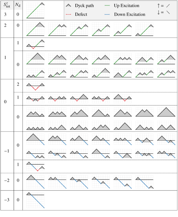
A Dyck path of even length $N=2n$ is a lattice path in the two-dimensional Cartesian plane with traversal from $(0,0)$ to $(n,n)$ in unit steps—either $(1,0)$ or $(0,1)$—and with the additional constraint that the path never crosses the line $y=x$. In the equivalent landscape picture, the allowed steps are the diagonals $(1,1)$ or $(1,-1)$, and the path going from $(0,0)$ to $(2n,0)$ never drops below the horizon (the line $y=0$). The number of unique Dyck paths of length $2n$ is a sequence of numbers called the Catalan number. The Catalan number of order $n$ is given by

The Hamiltonian of the Fredkin spin chain commutes with $S^{z}_{\text{tot}}=(1/2)\sum_{i=1}^{N}\sigma^{z}_{i}$, and hence the $S^{z}_{\text{tot}}$ is a good quantum number. The set of valid Dyck paths is a subspace within the $S^{z}_{\text{tot}}=0$ spin sector of the Hilbert space. The full Hilbert space consists of all spin assignments with $\sigma^{z}_{1}=+1$, $\sigma^{z}_{N}=-1$, and $\sigma^{z}_{i}=\pm 1$ at sites $1<i<N$. This corresponds to all random walks of the height profile starting from $h_{0}=0$ and ending at height $h_{N}=2S^{z}_{\text{tot}}$.

In order to describe the full Hilbert space, we introduce two additional concepts: excitations and defects. There is some flexibility in how one defines these. In this paper, we adopt the convention illustrated in Table 1. Each Dyck path is in 1–1 correspondence with a Dyck word that consists of equal numbers of properly nested left and right parentheses. Although a state in Dyck form or with one or more defects can present in any spin sector, excitations only occur in the $S^{z}_{\text{tot}}\neq 0$ spin sectors—with up excitations only in the $S^{z}_{\text{tot}}>0$ sectors and down excitations only in those with $S^{z}_{\text{tot}}<0$. To ensure a unique delimiter representation of the states, we establish the following prescription.

The population of excited bonds is fixed within each spin projection sector $S^{z}_{\text{tot}}\in\{0,\pm 1,\cdots,\pm(N/2-1)\}$. The excitations are

in number and connect (reading left to right) sites of odd and even index, consistent with the boundary conditions. Unlike the conventional $\hskip 1.00006pt(\hskip 1.00006pt\hskip 1.00006pt)\hskip 1.00006pt$ pairs, excitations themselves cannot be nested; i.e, $\hskip 1.00006pt{\color[rgb]{0,0.5,0}\lceil}\hskip 1.00006pt\hskip 1.00006pt{\color[rgb]{0,0.5,0}\rceil}\hskip 1.00006pt\hskip 1.00006pt{\color[rgb]{0,0.5,0}\lceil}\hskip 1.00006pt\hskip 1.00006pt{\color[rgb]{0,0.5,0}\rceil}\hskip 1.00006pt$ is allowed but $\hskip 1.00006pt{\color[rgb]{0,0.5,0}\lceil}\hskip 1.00006pt\hskip 1.00006pt{\color[rgb]{0,0.5,0}\lceil}\hskip 1.00006pt\hskip 1.00006pt{\color[rgb]{0,0.5,0}\rceil}\hskip 1.00006pt\hskip 1.00006pt{\color[rgb]{0,0.5,0}\rceil}\hskip 1.00006pt$ is not. Moreover, the representation can accommodate up to $N/2-1-N_{e}$ defects, organized in perfectly nested form: i.e., $\hskip 1.00006pt{\color[rgb]{0.87,0.09,0.12}\langle}\hskip 1.00006pt\hskip 1.00006pt{\color[rgb]{0.87,0.09,0.12}\langle}\hskip 1.00006pt\hskip 1.00006pt{\color[rgb]{0.87,0.09,0.12}\rangle}\hskip 1.00006pt\hskip 1.00006pt{\color[rgb]{0.87,0.09,0.12}\rangle}\hskip 1.00006pt$ is allowed but $\hskip 1.00006pt{\color[rgb]{0.87,0.09,0.12}\langle}\hskip 1.00006pt\hskip 1.00006pt{\color[rgb]{0.87,0.09,0.12}\rangle}\hskip 1.00006pt\hskip 1.00006pt{\color[rgb]{0.87,0.09,0.12}\langle}\hskip 1.00006pt\hskip 1.00006pt{\color[rgb]{0.87,0.09,0.12}\rangle}\hskip 1.00006pt$ is not. Defects occupy a position exclusively to the left (right) of the up (down) excitations. Given a particular spin configuration, it is straightforward to determine the number of defect bonds that must appear. We define left-cumulative and right-cumulative height functions,

such that $h_{0}=0$ and $h_{N}=2S^{z}_{\text{tot}}$ (whereas $\bar{h}_{0}=2S^{z}_{\text{tot}}$ and $\bar{h}_{N}=0$). The number of defects $N_{\text{d}}$ is then

The remaining spins that are not participating in an excitation or defect are grouped into disjoint chain segments, each of which must contain a spin configuration that is a Dyck word.

We have confirmed that the three-site correlated interaction that appears in our two-parameter tunable model preserves bond type, so that the number of excitations $N_{\text{e}}$ and the number of defects $N_{\text{d}}$ are good quantum numbers. Hence the reshuffling of short bonds by the Hamiltonian can be used to define a canonical form for each equivalence class of states:

Here, $N_{\text{e}}$, $N_{\text{d}}$, $N/2-N_{\text{d}}-N_{\text{e}}$ represent the pair counts of matching square-cornered brackets, angled brackets, and parentheses; these take on whole number values, limited only by the finite length of the spin chain and by the constraints imposed by the hard boundary conditions. The number of spins belonging to each delimiter type, $2N_{\text{e}}$ and $2N_{\text{d}}$ and $N-2N_{\text{d}}-2N_{\text{e}}$, is always even. Up-canted excitations cannot reach the right edge of the spin chain ($\hskip 1.00006pt{\color[rgb]{0,0.5,0}\rceil}\hskip 1.00006pt_{i}:i\neq N$), and down-canted excitations cannot reach the left ($\hskip 1.00006pt{\color[rgb]{0,0.38,0.68}\rfloor}\hskip 1.00006pt_{i}:i\neq 1$); hence the lone $\hskip 1.00006pt(\hskip 1.00006pt\hskip 1.00006pt)\hskip 1.00006pt$ pair on the right and left edges in Eqs. (9a) and (9b). Defects cannot extend to either end ($\hskip 1.00006pt{\color[rgb]{0.87,0.09,0.12}\langle}\hskip 1.00006pt_{i}\cdots\hskip 1.00006pt{\color[rgb]{0.87,0.09,0.12}\rangle}\hskip 1.00006pt_{\!j}:i\neq 1,j\neq N$).

The full Hilbert space for system size $N=8$ is shown in Fig. 2 using the landscape representation with up ($\diagup$) and down ($\diagdown$) slopes. The two lowest-energy states of the two-parameter model defined by Eq. (3) live in the subspace $(S^{z}_{\text{tot}},N_{d})\in\{(0,0),(0,1),(\pm 1,0)\}.$ With the exception of the two domes, the GS is of Dyck form and corresponds to ($S^{z}_{\text{tot}}=0,N_{\text{d}}=0$). The other important states belong to either ($S^{z}_{\text{tot}}=0,N_{\text{d}}=1$) or ($S^{z}_{\text{tot}}=\pm 1,N_{\text{d}}=0$), both of which can be represented in terms of a single defect or excitation by

Here, $\lvert i,j;\mathcal{D}^{\prime},\mathcal{D}^{\prime\prime},\mathcal{D}^{\prime\prime\prime}\rangle$ is a shorthand notation for the spin configuration $\lvert\mathcal{D}^{\prime}\rangle\otimes\lvert\sigma_{i}\rangle\otimes\lvert\mathcal{D}^{\prime\prime}\rangle\otimes\lvert\sigma_{j}\rangle\otimes\lvert\mathcal{D}^{\prime\prime\prime}\rangle$, and g = $g_{ij}(\mathcal{D}^{\prime},\mathcal{D}^{\prime\prime},\mathcal{D}^{\prime\prime\prime})$ is the corresponding wave function amplitude. The bond of is positioned at sites $i$ and $j$ and has ($\sigma_{i},\sigma_{j})\in\{\>\hskip 1.00006pt{\color[rgb]{0,0.5,0}\lceil}\hskip 1.00006pt\,\hskip 1.00006pt{\color[rgb]{0,0.5,0}\rceil}\hskip 1.00006pt,\hskip 1.00006pt{\color[rgb]{0,0.38,0.68}\lfloor}\hskip 1.00006pt\,\hskip 1.00006pt{\color[rgb]{0,0.38,0.68}\rfloor}\hskip 1.00006pt,\hskip 1.00006pt{\color[rgb]{0.87,0.09,0.12}\langle}\hskip 1.00006pt\,\hskip 1.00006pt{\color[rgb]{0.87,0.09,0.12}\rangle}\hskip 1.00006pt\>\}$ as appropriate. The length of the Dyck words $\mathcal{D}^{\prime},\mathcal{D}^{\prime\prime}$, and $\mathcal{D}^{\prime\prime\prime}$ are $i-1$, $j-i-1$, and $N-j$, respectively. The allowed values of (odd) $i$ and (even) $j$ are as follows:

The total number of allowed configurations is

For example, in the $N=8$ system with a single defect bond, there are five contributing states, and Eq. (10) takes the form

with normalization $N_{\text{norm}}=\sum_{n=1}^{N^{\text{conf}}}g_{n}^{2}$. Recall that the strong external boundary fields, which demand that $\sigma^{z}_{1}=+1$ and $\sigma^{z}_{N}=-1$, prevent the defect from touching either edge of the spin chain.

Exact diagonalization (ED) is implemented as described in Ref. Adhikari and Beach 2019. The basis-size reduction due to the discrete symmetries is not enough to significantly reduce the computational cost, so we cannot simulate large systems. To help guide our investigations, however, we have generated the full set of energy eigenstates for $N=12$ and $N=16$ over a densely spaced mesh of ($r,\theta$) values.

To access larger sizes, we employ a DMRG algorithm implemented in the open-source C++ library ITensor Fishman et al., taking advantage of the fact that $S^{z}_{\text{tot}}$ is a good quantum number in the model. We are mindful of the fact that the high level of entanglement in the vicinity of the Fredkin model and its mirror point at the “south pole” ($r\geq 1$ and $90^{\circ}\leq\theta\lesssim 110^{\circ}$ or $250^{\circ}\lesssim\theta\leq 270^{\circ}$) requires us to keep many states; farther away, we can be more cavalier about truncating the DMRG basis set. We are also careful about issues of convergence: in and around the two domes of the phase diagram (roughly corresponding to a region $1\leq r\lesssim 1.2$ and $110^{\circ}\lesssim\theta\lesssim 260^{\circ}$) an unexpectedly large number of sweeps is required, because the low-lying energy levels are very closely spaced (see Fig. 3).

Moreover, the convergence is strongly biased by the choice of initial trial state, because the nature of the low-lying states sometimes changes abruptly with a small change in $r$ or $\theta$ values. As a workaround, we make a list of possible low energy configurations using ED results for $N\leq 16$. Comparable configurations are then used to seed the DMRG calculations for bigger system sizes. The first excited state belongs to the $S^{z}_{\text{tot}}(\text{ES})=0$ spin sector in most parts of this region. So, we calculated the two orthogonal states in $S^{z}_{\text{tot}}=0$ having the lowest eigenvalues using many possible trial states. Then, the ground state and the first excited state are found by sorting two lowest energies in the $S^{z}_{\text{tot}}=0$ spin sector and the lowest energy in the $S^{z}_{\text{tot}}=1$ spin sector.

We have employed a very conservative convergence criterion: the DMRG algorithm runs through $10N$ sweeps using an adaptive truncation cutoff at relative error $10^{-12}$ with maximum bond dimension $15N$. We have benchmarked our DMRG results to near double-precision floating-point accuracy against ED results for $N\leq 16$. The DMRG computation is carried out for all lattice sizes that are multiples of 4 up to $N=60$, over a tight mesh of tuning parameter values $r=0,0.025,\ldots,2.975,3$ and $\theta=0^{\circ},1^{\circ},\ldots,359^{\circ},360^{\circ}$. The most expensive of those simulations corresponds to $600$ sweeps with a maximum bond dimension of 900. Various physical quantities are computed in the ground state as a function of the tuning parameters $r,\theta$; i.e., $O(r,\theta)=\langle\hat{O}\rangle=\langle\psi_{0}(r,\theta)\rvert\hat{O}\lvert\psi_{0}(r,\theta)\rangle$. These include the spin profile $\langle\sigma_{i}^{z}\rangle$, dimer profile $\langle\sigma_{i}^{z}\sigma_{i+1}^{z}\rangle-\langle\sigma_{j}^{z}\rangle\langle\sigma_{j+1}^{z}\rangle$, dimer order parameter

where

Ising ferromagnetic order parameter (z FM)

Ising antiferromagnetic order parameter (z AFM)

doubly staggered Ising magnetic order parameter (z DSM)

where

the xy-plane ferromagnetic order parameter (xy FM)

and the xy-plane antiferromagnetic order parameter (xy AFM)

Unlike the upper half-plane where wave function amplitudes are all positive, the wave function amplitudes in the lower circular plane contain an admixture of positive and negative signs. About the horizontal line ($\gamma=0$), diagonal ($\sigma^{z}$ dependent only) and off-diagonal (products of $\sigma^{+}$ and $\sigma^{-}$) measurements are symmetric and antisymmetric, respectively. For example, xy FM and xy AFM measurements in Fig. 6(b) have peaks at $(r,\theta)=(1,90^{\circ})$ and $(1,270^{\circ})$, respectively. So, we discuss our diagonal measurement results only for the upper semicircular plane, and a similar explanation applies to the lower semicircular plane. We analyze the ground state properties of the system at distinct regions of the phase space separately in the Secs. V.1–V.4.

In Sec. III, we discussed how to represent the Hilbert space using the language of matching and nested spin pairs. Conventional pairs, with a spin up to the left and spin down to the right, are the building blocks of the Dyck word ground state. By promoting certain conventional bonds to a bond of different character—either an excited bond that cants the spin state out of the xy plane or a defect bond that carries a Dyck word mismatch—we were able to cover the entire Hilbert space. We derived formulas relating the number of excited and defect bonds to the explicit spin arrangement in a given state, and we offered a detailed prescription for converting from the raw spin representation into the bond representation. Most important, we argued that the population count for each kind of bond is a good quantum number for the model Hamiltonian considered in Sec. II

Figure 1 shows a summary of the zero-temperature quantum phase diagram, based on an extrapolation of various numerical measurements on finite-size systems to the thermodynamic limit. The diagonal measurements (those involving $\sigma^{z}$ only) are symmetric about the horizontal $(\gamma=0$) axis, whereas off-diagonal measurements (involving $\sigma^{+}$ and $\sigma^{-}$) are antisymmetric. The two-parameter extended model we have proposed is exactly solvable on the horizontal line ($\gamma=0$) and on the unit circle ($\eta^{2}+\gamma^{2}=1$). For $r<1$, the ferromagnetic ground state is doubly degenerate. For $r\geq 1$, the ground state is everywhere unique, except at the point $(r=1,\theta=180^{\circ})$, for all system sizes satisfying $N=0\ (\text{mod}\,4)$. Along the line $(r>1,\theta=180^{\circ})$, the ground state is highly degenerate for sizes $N=2\ (\text{mod}\,4)$, since the desired doubly staggered pattern is prevented from forming; hence, these sizes are excluded.

The $t$-deformed model lies on the unit circle, and the line $\eta=0$ separates the gapped, ordered phases on the right from the gapless, disordered phases on the left. The latter belong to a region in which the excitation gap closes exponentially fast. That unit circle also demarcates a boundary between regions that show ferromagnetic behavior inside and coexistence of antiferromagnetic and dimerized behavior elsewhere. The dimer order is strong in the upper and lower parts of the diagram, where quantum fluctuations are enhanced. On the other hand, the right part of the phase space favors z AFM behavior and the left supports z DSM behavior. The system is gapped everywhere except on ellipses inside the unit circle and on the boundary of the domes on the left part of the phase diagram. Most parts of the phase space favor the Fredkin-like Dyck-form ground state except the two domes and inside the unit circle. The two domes on the left and the Dyck-form $(S^{z}_{\text{tot}}=0,N_{\text{d}}=0)$ excitation on the top of the phase diagram both emerge only for $N\geq 10$; in the thermodynamic limit, they all touch the circle at $r\approx 1.7$, approaching it from opposite sides. Inside the two domes, the ground state favors $S^{z}_{\text{tot}}=0$ and $N_{\text{d}}=1$, leaving Dyck-form to the higher energy state. Inside the unit circle, the ground state is ferromagnetic (higher $\lvert S^{z}_{\text{tot}}\rvert$) with no defects ($N_{\text{d}}=0$).

The tunable Hamiltonian we have proposed and studied in this paper puts the Fredkin model and its $t$-deformed generalization in the context of a larger space of models that have a well-define notion of conventional, excited, and defect bonds. This is interesting because the identification of the bond character relies on knowledge of the complete spin configuration; in other words it is a global rather than local property of the spin state and hence has a topological nature. Our work makes clear that, even though the $t$ deformation is frustration free, its quantum-disordered ground state is nonetheless a result of a special tuning of the competing interactions, one that carefully balances their ferromagnetic and antiferromagnetic tendencies.

References

- Haseda and Miedema (1961) T. Haseda and A. R. Miedema, “Specific heat of Cu(NH3)4SO4H2O below 1K,” Physica 27, 1102 (1961).
- Flippen and Friedberg (1963) R. B. Flippen and S. A. Friedberg, “Low-temperature magnetic susceptibilities of some hydrated formates of Cu++ and Mn++,” The Journal of Chemical Physics 38, 2652 (1963).
- Wagner and Friedberg (1964) G. R. Wagner and S. A. Friedberg, “Linear chain antiferromagnetism in Mn(HCOO)22H2O,” Physics Letters 9, 11 (1964).
- Hone et al. (1974) Daniel Hone, Claudio Scherer, and Ferdinando Borsa, “Proton spin-lattice relaxation in TMMC [(CH3)4 NMnCl3],” Physical Review B 9, 965 (1974).
- Borsa and Mali (1974) F. Borsa and M. Mali, “Experimental study of high-temperature spin dynamics in one-dimensional heisenberg paramagnets,” Physical Review B 9, 2215 (1974).
- Motoyama et al. (1996) N. Motoyama, H. Eisaki, and S. Uchida, “Magnetic Susceptibility of Ideal Spin-1/2 Heisenberg Antiferromagnetic Chain Systems, Sr2CuO3 and SrCuO2,” Physical Review Letters 76, 3212 (1996).
- Bitko et al. (1996) D. Bitko, T. F. Rosenbaum, and G. Aeppli, “Quantum Critical Behavior for a Model Magnet,” Physical Review Letters 77, 940 (1996).
- Coldea et al. (2010) R. Coldea, D. A. Tennant, E. M. Wheeler, E. Wawrzynska, D. Prabhakaran, M. Telling, K. Habicht, P. Smeibidl, and K. Kiefer, “Quantum criticality in an ising chain: Experimental evidence for emergent E8 symmetry,” Science 327, 177 (2010).
- Breunig et al. (2017) Oliver Breunig, Markus Garst, Andreas Klümper, Jens Rohrkamp, Mark M. Turnbull, and Thomas Lorenz, “Quantum criticality in the spin-1/2 Heisenberg chain system copper pyrazine dinitrate,” Science Advances 3, eaao3773 (2017).
- Zaliznyak et al. (1999) I. A. Zaliznyak, C. Broholm, M. Kibune, M. Nohara, and H. Takagi, “Anisotropic Spin Freezing in the Zigzag Chain Compound SrCuO2,” Physical Review Letters 83, 5370 (1999).
- Auerbach (2012) A. Auerbach, Interacting Electrons and Quantum Magnetism, Graduate Texts in Contemporary Physics (Springer New York, 2012).
- Kojima et al. (1997) K. M. Kojima, Y. Fudamoto, M. Larkin, G. M. Luke, J. Merrin, B. Nachumi, Y. J. Uemura, N. Motoyama, H. Eisaki, S. Uchida, K. Yamada, Y. Endoh, S. Hosoya, B. J. Sternlieb, and G. Shirane, “Reduction of Ordered Moment and Néel Temperature of Quasi-One-Dimensional Antiferromagnets Sr2CuO3 and Ca2CuO3,” Physical Review Letters 78, 1787 (1997).
- Bursill et al. (1995) R. Bursill, G. A. Gehring, D. J. J. Farnell, J. B. Parkinson, Tao Xiang, and Chen Zeng, “Numerical and approximate analytical results for the frustrated spin-1/2 quantum spin chain,” Journal of Physics: Condensed Matter 7, 8605 (1995).
- Jafari and Langari (2007) R. Jafari and A. Langari, “Phase diagram of the one-dimensional XXZ model with ferromagnetic nearest-neighbor and antiferromagnetic next-nearest-neighbor interactions,” Physical Review B 76, 014412 (2007).
- Wierschem and Sengupta (2014) Keola Wierschem and Pinaki Sengupta, “Characterizing the Haldane phase in quasi-one-dimensional spin-1 Heisenberg antiferromagnets,” Modern Physics Letters B 28, 1430017 (2014).
- Sachdev (2011) Subir Sachdev, Quantum Phase Transitions, 2nd ed. (Cambridge University Press, 2011).
- Hirano et al. (2008) T. Hirano, H. Katsura, and Y. Hatsugai, “Topological classification of gapped spin chains: Quantized Berry phase as a local order parameter,” Physical Review B 77, 094431 (2008).
- Pollmann et al. (2012) Frank Pollmann, Erez Berg, Ari M. Turner, and Masaki Oshikawa, “Symmetry protection of topological phases in one-dimensional quantum spin systems,” Physical Review B 85, 075125 (2012).
- Lieb et al. (1961) Elliott Lieb, Theodore Schultz, and Daniel Mattis, “Two soluble models of an antiferromagnetic chain,” Annals of Physics 16, 407 (1961).
- Latorre et al. (2004) Jose I. Latorre, E. Rico, and G. Vidal, “Ground state entanglement in quantum spin chains,” Quantum Information & Computation 4, 48 (2004).
- Keating and Mezzadri (2005) J. P. Keating and F. Mezzadri, “Entanglement in Quantum Spin Chains, Symmetry Classes of Random Matrices, and Conformal Field Theory,” Physical Review Letters 94, 050501 (2005).
- Haldane (1983) F. D. M. Haldane, “Nonlinear Field Theory of Large-Spin Heisenberg Antiferromagnets: Semiclassically Quantized Solitons of the One-Dimensional Easy-Axis Néel state,” Physical Review Letters 50, 1153 (1983).
- Haldane (2017) F. Duncan M. Haldane, “Nobel lecture: Topological quantum matter,” Review of Modern Physics 89, 040502 (2017).
- Affleck and Haldane (1987) Ian Affleck and F. D. M. Haldane, “Critical theory of quantum spin chains,” Physical Review B 36, 5291 (1987).
- Sirker et al. (2011) J. Sirker, V. Y. Krivnov, D. V. Dmitriev, A. Herzog, O. Janson, S. Nishimoto, S.-L. Drechsler, and J. Richter, “– Heisenberg model at and close to its quantum critical point,” Physical Review B 84, 144403 (2011).
- Patil et al. (2017) Pranay Patil, Ying Tang, Emanuel Katz, and Anders W. Sandvik, “Indicators of conformal field theory: Entanglement entropy and multiple-point correlators,” Physical Review B 96, 045140 (2017).
- Hirobe et al. (2017) Daichi Hirobe, Masahiro Sato, Takayuki Kawamata, Yuki Shiomi, Ken-ichi Uchida, Ryo Iguchi, Yoji Koike, Sadamichi Maekawa, and Eiji Saitoh, “One-dimensional spinon spin currents,” Nature Physics 13, 30 (2017).
- Bose (2003) Sougato Bose, “Quantum Communication through an Unmodulated Spin Chain,” Physical Review Letters 91, 207901 (2003).
- Barjaktarevic et al. (2005) J. P. Barjaktarevic, R. H. McKenzie, J. Links, and G. J. Milburn, “Measurement-Based Teleportation along Quantum Spin Chains,” Physical Review Letters 95, 230501 (2005).
- Zhou et al. (2002) Xingxiang Zhou, Zheng-Wei Zhou, Guang-Can Guo, and Marc J. Feldman, “Quantum Computation with Untunable Couplings,” Physical Review Letters 89, 197903 (2002).
- Bartlett et al. (2010) Stephen D. Bartlett, Gavin K. Brennen, Akimasa Miyake, and Joseph M. Renes, “Quantum Computational Renormalization in the Haldane Phase,” Physical Review Letters 105, 110502 (2010).
- Simon et al. (2011) Jonathan Simon, Waseem S. Bakr, Ruichao Ma, M. Eric Tai, Philipp M. Preiss, and Markus Greiner, “Quantum simulation of antiferromagnetic spin chains in an optical lattice,” Nature (London) 472, 307 (2011).
- Choi et al. (2019) Deung-Jang Choi, Nicolas Lorente, Jens Wiebe, Kirsten von Bergmann, Alexander F. Otte, and Andreas J. Heinrich, “Colloquium: Atomic spin chains on surfaces,” Reviews of Modern Physics 91, 041001 (2019).
- Movassagh and Shor (2016) Ramis Movassagh and Peter W. Shor, “Supercritical entanglement in local systems: Counterexample to the area law for quantum matter,” Proceedings of the National Academy of Sciences 113, 13278 (2016).
- Movassagh (2018) Ramis Movassagh, “The gap of Fredkin quantum spin chain is polynomially small,” Annals of Mathematical Sciences and Applications 3, 531 (2018).
- Bravyi et al. (2012) Sergey Bravyi, Libor Caha, Ramis Movassagh, Daniel Nagaj, and Peter W. Shor, “Criticality without Frustration for Quantum Spin-1 Chains,” Physical Review Letters 109, 207202 (2012).
- Movassagh (2017) Ramis Movassagh, “Entanglement and correlation functions of the quantum Motzkin spin-chain,” Journal of Mathematical Physics 58, 031901 (2017).
- Dell’Anna et al. (2016) L. Dell’Anna, O. Salberger, L. Barbiero, A. Trombettoni, and V. E. Korepin, “Violation of cluster decomposition and absence of light cones in local integer and half-integer spin chains,” Physical Review B 94, 155140 (2016).
- Chen et al. (2017a) Xiao Chen, Eduardo Fradkin, and William Witczak-Krempa, “Quantum spin chains with multiple dynamics,” Physical Review B 96, 180402 (2017a).
- Chen et al. (2017b) Xiao Chen, Eduardo Fradkin, and William Witczak-Krempa, “Gapless quantum spin chains: multiple dynamics and conformal wavefunctions,” Journal of Physics A: Mathematical and Theoretical 50, 464002 (2017b).
- Zhang et al. (2017) Zhao Zhang, Amr Ahmadain, and Israel Klich, “Novel quantum phase transition from bounded to extensive entanglement,” Proceedings of the National Academy of Sciences 114, 5142 (2017).
- Zhang and Klich (2017) Zhao Zhang and Israel Klich, “Entropy, gap and a multi-parameter deformation of the Fredkin spin chain,” Journal of Physics A: Mathematical and Theoretical 50, 425201 (2017).
- Levine and Movassagh (2017) Lionel Levine and Ramis Movassagh, “The gap of the area-weighted Motzkin spin chain is exponentially small,” Journal of Physics A: Mathematical and Theoretical 50, 255302 (2017).
- Udagawa and Katsura (2017) Takuma Udagawa and Hosho Katsura, “Finite-size gap, magnetization, and entanglement of deformed Fredkin spin chain,” Journal of Physics A: Mathematical and Theoretical 50, 405002 (2017).
- Padmanabhan et al. (2019) Pramod Padmanabhan, Fumihiko Sugino, and Vladimir Korepin, “Quantum phase transitions and localization in semigroup Fredkin spin chain,” Quantum Information Processing 18, 69 (2019).
- Salberger et al. (2017) Olof Salberger, Takuma Udagawa, Zhao Zhang, Hosho Katsura, Israel Klich, and Vladimir Korepin, “Deformed Fredkin spin chain with extensive entanglement,” Journal of Statistical Mechanics: Theory and Experiment 2017, 063103 (2017).
- Adhikari and Beach (2019) Khagendra Adhikari and K. S. D. Beach, “Deforming the Fredkin spin chain away from its frustration-free point,” Physical Review B 99, 054436 (2019).
- Alexander et al. (2019) Rafael N. Alexander, Amr Ahmadain, Zhao Zhang, and Israel Klich, “Exact rainbow tensor networks for the colorful Motzkin and Fredkin spin chains,” Physical Review B 100, 214430 (2019).
- Dell’Anna (2019) Luca Dell’Anna, “Long-distance entanglement in Motzkin and Fredkin spin chains,” SciPost Physics 7, 53 (2019).
- Sugino and Korepin (2018) Fumihiko Sugino and Vladimir Korepin, “Rényi entropy of highly entangled spin chains,” International Journal of Modern Physics B 32, 1850306 (2018).
- (51) Libor Caha and Daniel Nagaj, “The pair-flip model: a very entangled translationally invariant spin chain,” arXiv:1805.07168 .
- Salberger and Korepin (2017) Olof Salberger and Vladimir Korepin, “Entangled spin chain,” Reviews in Mathematical Physics 29, 1750031 (2017).
- Barbiero et al. (2017) L. Barbiero, L. Dell’Anna, A. Trombettoni, and V. E. Korepin, “Haldane topological orders in Motzkin spin chains,” Physical Review B 96, 180404 (2017).
- (54) Giovanni Ramírez, Javier Rodríguez-Laguna, and Germán Sierra, “Entanglement over the rainbow,” Journal of Statistical Mechanics: Theory and Experiment 2015, P06002.
- Ramires (2019) Aline Ramires, “Frustration can be critical,” Nature Physics 15, 1212 (2019).
- Zhao et al. (2019) Hengcan Zhao, Jiahao Zhang, Meng Lyu, Sebastian Bachus, Yoshifumi Tokiwa, Philipp Gegenwart, Shuai Zhang, Jinguang Cheng, Yi-feng Yang, Genfu Chen, Yosikazu Isikawa, Qimiao Si, Frank Steglich, and Peijie Sun, “Quantum-critical phase from frustrated magnetism in a strongly correlated metal,” Nature Physics 15, 1261 (2019).
- (57) Matthew Fishman, Steven R. White, and E. Miles Stoudenmire, “The ITensor software library for tensor network calculations,” arXiv:2007.14822 .
- Lemm and Mozgunov (2019) Marius Lemm and Evgeny Mozgunov, “Spectral gaps of frustration-free spin systems with boundary,” Journal of Mathematical Physics 60, 051901 (2019).