Super efficient geodesics in the complex of curves
Abstract.
We introduce a subclass of the efficient geodesics, called super efficient geodesics, that the bound of intersection number in the initial efficiency only depends on the genus of surface. For any two vertices, , in the complex of curves of a closed oriented surface of genus , and any efficient geodesic, , it was previously established by Birman, Margalit and the second author [5] that there is an explicitly computable list of at most candidates for the vertex. In this note we establish a bound for this computable list for the super efficient geodesics that is independent of d-distance and only dependent on genus. The proof relies on an intersection growth inequality (IGI) between the intersection number of two curves and their distance in the complex of curves, together with a thorough analysis of the dot graph associated with the intersection sequence.
Key words and phrases:
complex of curves, efficient geodesics, intersection growth inequality, super efficient geodesics, super efficiency.2010 Mathematics Subject Classification
Primary: 57M60. Secondary: 20F38.1. Introduction
1.1. Initial background
Let be a closed oriented surface of genus . The complex of curves or curve complex of the surface is a simplicial complex such that each vertex corresponds to the isotopy class of an essential simple closed curve, and vertices form an -simplex of if their representatives can be realized disjointly. At times we will use the words “vertices” and “curves” interchangeably, and use curve as essential simple closed curve. For any two curves and in , the distance is the minimal number of edges in connecting to . A geodesic in is a sequence of vertices such that for all .
Harvey [9] introduced the curve complex in 1978 as a tool for studying the mapping class group of surfaces. In 1996, Masur and Minsky [12] proved the seminal result that is -hyperbolic. However, the computation of distance in is still very intimidating. The first attempt of such algorithm was due to Leasure [11] in his thesis in 2002. After that, there are several other algorithms found by Shackleton [14], Watanabe [15] and Webb [16], in which all algorithms utilize the notion of tight geodesics that were first constructed in a sequel [13] of Masur-Minky’s work [12]. In [5] Birman-Margalit-Menasco introduce efficient geodesics, an alternative finite set of geodesics for computing the distance in .
To elaborate, suppose is a geodesic of length in , and are associated curve representatives in . Initially focussing on the triple, , assume that they pairwise are in minimal position—, and no subarc of or is cobounding a bigon disc with a subarc of . A reference arc for is an arc, , that is in minimal position with —again, no cobounding a bigon disc between and . The geodesic is initially efficient if for all possible reference arcs. Moreover, the geodesic is called efficient, if the oriented geodesic is initially efficient for and the oriented geodesic is also initially efficient.
The existence of initially efficient geodesics is established in [5]. Specifically, it is shown that there that an explicitly computable list of at most
vertices, , which can appear as the first vertex of an (initially) efficient geodesic . In [5] it is argued that any geodesic could be replaced by an initially efficient geodesic; that is, , for all possible reference arcs . Here, the notation refers to the number of minimal intersections which is achieved when there is no cobounding bigon disc. Equivalently, when and intersect minimally within the isotopy class .
1.2. Main results
Our key advancement in this note is the establishment of a subclass of initially efficient geodesics, called initially super efficient geodesics, for which the intersection bound with the reference arcs is for genus and for . The super efficient geodesics follow similarly as the efficient geodesics in [5] once we establish the initially super efficient geodesics. In particular, the existence of initially super efficient geodesics comes from changing the distance-dependent intersection bound to one that is dominated by a linear function of genus.
Theorem 1.1.
Let and be two vertices in with distance . There exists an (initially) super efficient geodesic in connecting and . More precisely, suppose , and are minimally intersecting representatives of , and , respectively. Let be any reference arc for the pair . Then for , we have ; and for , we have .
For a pair of curves, , associated with a pair of vertices, , we again assume and are in minimal position. Define . The complexity of a path, in is then defined to be the number, . Then, among the geodesics between two vertices, we have the following inclusion relation,
where the ISEG stands for initially super efficient geodesics and the IEG stands for initially efficient geodesics.
Now building on Theorem 1.1 we obtain a new bound on the size of this explicit list of the candidates for vertex in the initially super efficient geodesics that is independent of distance and only dependent on genus. In particular, we have the following corollary.
Corollary 1.2 (Super efficiency).
If is an (initially) super efficient geodesic of with , then, for , there is an explicitly computable list of at most
vertices that can appear as the first vertex on an (initially) super efficient geodesic. When the bound on this list is .
1.3. Test for a geodesic path
The new idea advancing our understanding of efficient geodesics is the application of a simple necessary condition for when a given vertex sequence is a geodesic. Specially, for a pair of natural numbers, with and , define the minimal intersection function, . Currently, few exact values of are known. We do know the and for we know that [2]. (Recall, pairs of curves at distance or greater are called filling pairs.) Additional, we know that [8].
Now, let we a sequence of essential simple curves in representing the vertices of such that for all . If is a geodesic, by definition . But, this implies that . This observation gives us a necessary test for (and ) being a geodesic sequence. Additionally, we can expand on this necessary test by utilizing the triangle inequality. Specially, for any curve we cannot have
| (1) |
The argument in [5] for the existence of efficient geodesics comes from the application of “path surgery” operations which replaces a geodesic with a new geodesic path, , while strictly decreasing the intersections of representative curves with reference arcs. In the proof the fact that the new sequence, , is a geodesic only comes from it being the same length as . Our strategy for proving Theorem 1.1 is to show that if the intersection of with a reference arc is too large then, in order that there not be a curve satisfying equation 1, our geodesic path is of infinite length. To implement this strategy we need a tight lower bound on the growth of as a function of d. Our bound will be given by the intersection growth inequality or IGI.
Theorem 1.3 (IGI).
Let two curves represent two vertices that realize their intersection number. If and then
In particular, . If and then
that is,
In particular, for .
1.4. An aside—other lower bounds for
The IGI takes into account of the genus of surface improving the following estimate given by Hempel [10]:
| (2) |
Another estimate utilizes the topology of a surface was proved by Bowditch (Corollary 2.2 in [6]) and reformulated by Aougab, Patel and Taylor [3].
Theorem 1.4.
For any two curves and on an oriented surface with Euler characteristic and ,
| (3) |
From the asymptotic perspective, a much stronger result was provided by Aougab (Theorem 1.2 in [1]) to show the uniform hyperbolicity of curve graphs.
Theorem 1.5.
For each , there is some such that if , whenever and ,
| (4) |
where .
For a closed oriented surface , Bowditch’s estimate becomes
If , then the upper bound in the IGI is smaller. Otherwise, Bowditch’s estimate is smaller as long as the intersection number of is sufficiently large. The bound in Theorem 1.1 is obtained with the IGI.
1.5. Improving distance algorithm
We extend the discussion begun in the introduction of [5] comparing the bounds on the size of the set of candidates given by the use of super efficient geodesics and the bounds by the use of tight geodesics. From that discussion we have the bound results coming from the work of Webb [16] which gives a bound of . In particular, when and we get a bound that is . Whereas, a super efficiency bound for is and independent of distance. Although an improvement, still such large bounds do not give a suitable understanding in how super efficient geodesics might be utilized in the implementation of an algorithm for computing distance.
In [4] Bell and Webb describe such a polynomial time algorithm based on the Masur-Minsky’s tight geodesics technology for computing distance in the curve complex. A key feature of their description is the “train-track-type” behavior of curves representing the vertices of a tight geodesic. A distance algorithm utilizing super efficient geodesics will exhibit analogous behavior in terms of “parallel arcs”, but in order to more fully expand the discussion in this direction it is helpful to have the reader understand the details of the proof of Theorem 1.1. We thus postpone this discussion until §8.
1.6. Outline of paper
The paper is organized as follows. In §2, we utilize the intersection number of a minimal filling pair as a lower bound and linear integer programming to establish the intersection growth inequality (IGI). In §3, we use the one-vertex triangulation of surface to show that some parallel arcs occur as the intersection number is sufficiently large. §4 reviews the techniques of efficient geodesics and curve surgery from [5]. In §5, we describe a “triangular shape” dot graph will occur in the worst scenario and its corresponding parallel arcs on the surface. §6 defines these parallel arcs as a rainbow and expands the dot graph machinery of [5] by investigating the pattern hided in the dot graph that arises as a rainbow, which allows us to calculate the minimal intersection number that will create another rainbow for other curves. We complete the proof of Theorem 1.1 by applying the IGI to the pattern of dot graph in the last §7. Then the super efficiency of Corollary 1.2 follows immediately. Finally, we revisit the discussion of how our results could be utilized in the implementation of a distance computing algorithm in §8.
Acknowledgement
The second author wishes to thank Dan Margalit for numerous conversations he had with him during the development of this project. Similarly, the second author thanks Joan Birman for numerous discussions on the curve complex and efficient geodesics. We also wish to thank Kasra Rafi for alerting us to Brian Bowditch’s growth rate result in [6], and thank Tarik Aougab for letting us know his asymptotic growth rate in Theorem 1.5 in [1]. Finally, we would like to thank an anonymous reviewer for pointing out an error in our original statement of Theorem 1.1 and many other helpful comments that improved the exposition.
2. Establishing the IGI
The idea of our proof for the IGI is to utilize the linear integer program (LIP) approach that was developed in the work of Glenn, Morrel, Morris and the second author [8] to establish the following result.
Theorem 2.1.
The minimal intersection number for a filling pair, , representing vertices , respectively, with is .
Proof of Theorem 1.3.
First, let us recall the LIP argument. Suppose that is a filling pair for , and we split along and consider the resulting properly embedded arcs of in a genus one surface having two boundary components, . (As in [5], we can reduce to the case where in non-separating so that the surface is connected.) Assume that and are arranged to being minimally intersecting up to isotopy, we can assume that all the discs of are -gons, . Now consider an essential curve, , that intersect each arc of at most once. We notice that has to be sufficient so that . In particular, if , we have to have , since is the minimal intersection number for the pair to be filling.
2pt \pinlabel at 116 100 \pinlabel at 107 245 \pinlabel at 340 123 \pinlabel at 73 305 \pinlabel at 380 305 \pinlabel at 225 90 \pinlabel at 625 93 \pinlabel at 619 245 \pinlabel at 840 123 \pinlabel at 585 305 \pinlabel at 885 305 \pinlabel at 735 94 \endlabellist
We can translate this above discussion into a system of linear inequalities, one for each such simple closed curve . First, in we can collapse all bands of -gon regions to a single properly embedded arc. This gives us a collection of non-parallel properly embedded essential arcs in . If need be we throw in additional essential arcs such that our collection, , is a maximal collection of non-parallel properly embedded essential arcs in . Such a maximal collection splits up into four -gon disc regions. (Up to homeomorphism there are only a finite number of ways gluing together four -gons to construct .) The left illustration in Figure 1 shows one possible -gon decomposition of . To find all possible loops, , of the required type that intersect any essential arc in our collection at most once, we consider the dual graph, , to this decomposition, as illustrated in the right of Figure 1. One of our needed curves is then just a circuit—a closed edge-path—in . To each such circuit we associate an inequality as follows.
First, assign weights, , to each of the six essential arcs in the decomposition. Each corresponds to the number of parallel arcs of . Next, for any circuit add together all the weights of the arcs of that the circuit intersects. For a circuit , this sum is equal to . Thus, by our previous discussion this sum is greater than when . The circuits of Figure 1 yield the following LIP system (2).
|
|
When we minimize constrained by LIP (2), we find that the minimum value of is , which is twice —the scaling factor of constrained by LIP (2). The minimum value of is achieved when and . (One can utilize https://www.easycalculation.com/ operations-research/simplex-method-calculator.php online.)
Remark 2.2.
In order to re-glue the two boundary curves of so that in we obtain the curve , it is necessary that the sum of the weight on each boundary curve to be equal—an added constraint to (2) that is currently missing. With such an added constraint, as noted in [8], any other -gon decomposition of will produce an LIP that is equivalent to LIP (2) up to relabeling. So the minimization of will still result in a value of .
By the linearity of LIP (2), if we replaced every occurrence of the lower bound of by and asked what would the minimal value of so constrained, our answer would be . Now the minimal intersection for a distance filling pair as stated in Theorem 2.1 is , not . This value was obtained by doing a search for distance filling pair utilizing the MICC program [7] that is an implementation of the efficient geodesic algorithm and this search was simplified by starting with filling pairs having at least intersections. Knowing this additional fact we can conclude that any distance filling pair of must have intersection number at least . And, in general we have our claimed inequality
for a filling pair of distance .
Finally, we consider a filling pair, for a higher genus and we split along to produce , we observe that there will always be an embedded in , for . Thus, when we produce a -gon decomposition for coming from a complete collection of non-parallel essential properly embedded arcs, the associated LIP for the dual graph will contain (up to relabeling) a copy of LLP (2). It follows that the scaling factor of —the sum of all the weights—is at least . This observation plus the fact that is the minimal intersection number for a filling pair yields the inequality:
∎
3. One-vertex triangulation and parallel arcs
Suppose is a geodesic of length in , and are representatives of that are pairwise in minimal position. For any reference arc of the pair , that is, an arc that is in minimal position with and whose interior is disjoint from . In fact, it suffices to look at the reference arc that connects the midpoints of -edges in a non-rectangular polygon of . In this section, we will show the existence of parallel arcs of given that the intersection between and is sufficiently large. We start off with a calculation of one-vertex triangulation of a closed surface .
Lemma 3.1.
The number of edges in one-vertex triangulation of a closed oriented surface is .
Proof.
Consider a one-vertex triangulation of with number of vertices, edges and faces denoted by , and , respectively. By Euler characteristic calculation, . In the triangulation, each face has 3 edges and each edge is shared by 2 faces, then we have . Since there is a unique vertex, if we multiply the Euler characteristic by 3, then
| (13) |
∎
Now focus on the components of . Two arc components are parallel in if they are two opposite sides of a rectangular disc—the other two sides being in . (See Figure 2.)
2pt
\pinlabel at 0 85
\pinlabel at 15 120
\pinlabel at 48 120
\pinlabel at 220 85
\pinlabel at 240 120
\pinlabel at 277 120
\endlabellist

We want to determine the minimal number of components of such that once the number of components is larger than , then the parallel arcs will occur. When we split along , the reference arc is a properly embedded arc with its endpoints on the boundary of the resulting surface, , where .
Lemma 3.2.
With the setup on a closed surface as above, if , then there exist parallel arcs of . More generally, if , then there exist at least parallel arcs of .
Proof.
There are three cases we need to consider:
- (1)
is non-separating and two endpoints of are on the two distinct boundary components of the connected surface ;
- (2)
is non-separating and both endpoints of are on the same boundary component of the connected surface ;
- (3)
is separating and two endpoints of is on the single boundary component of one of the two components in .

In all cases we can think of as being in a surface of at least one less genus with either one or two vertices (the boundary curves crushed to points). The Figures 3 & 4 are illustrated for the two cases in which the two intersection points of an arc are either of opposite orientations or of same orientation. In general, the two cases are mixed and the arcs are not necessarily parallel.
In Figures 3(1) and 4(1), the two endpoints of the arc are on two distinct boundary components of . The two boundary components are crushed to two points, and the arc is collapsed to a single point as well. It follows that the number of components of is same as the number of edges in one-vertex triangulation of surface . By Lemma 13, it is .
In the second case, Figures 3(2) and 4(2), both endpoints of are on the same boundary/vertex of . The reference arc will be one of the edges of a one-vertex triangulation of a once punctured . Since two more non-parallel edges are allowed to be added to the triangle containing the vertex crushed by the other boundary as illustrated in Figure 5. The number of components of is .
In the third case, the number of components of surpasses the second case. Hence, in all cases, the most possible number of non-parallel components of is .
The number of components of is the same as . If , then there must be at least two arcs of that are parallel. More generally, if , there must be at least parallel arcs by the Pigeonhole principle.
∎
4. Efficient geodesics
In this section, we will recall some fundamentals of the efficient geodesics from [5]. Let and be vertices of with and be a geodesic connecting to . The intersection between the representatives of and the reference arc produces a sequence of natural numbers along , which is called the intersection sequence of the along .
An intersection sequence of natural numbers can be arranged in a normal form called sawtooth form, that is,
If the intersection sequence of the curves along in sawtooth form is viewed as a function, , where is the cardinality of , then the graph is a set of lattice points of integer coordinates. The graph of the sequence is called dots, and the line segments resulting from the join of dots with slope 1 are called ascending segments. The resulting graph of intersection sequence in sawtooth form is called the dot graph, denoted by . An example of dot graph is illustrated in Figure 6.
Next, we will deal with certain shapes of polygons in the dot graph. A polygon in the plane is a dot graph polygon if
- (1)
the edges all have slope 0 or 1,
- (2)
the edges of slope 0 have nonzero length, and
- (3)
the vertices all have integer coordinates.
The edges of slope 1 in a dot graph polygon are called ascending edges and the edges of slope 0 are called horizontal edges.
Let be a sequence of natural numbers in sawtooth form. A dot graph polygon is a -polygon if:
- (1)
the vertices are dots of and
- (2)
the ascending edges are contained in ascending segments of .
A box in is a -quadrilateral with the following two properties:
- (1)
the leftmost ascending edge contains the highest point of some ascending segment of and
- (2)
the rightmost ascending edge contains the lowest point of some ascending segment of .
Up to translation and changing the edge lengths, there are four types of dot graph hexagons; two have an acute exterior angle, and we will not need to consider these. Notice that a dot graph hexagon necessarily has a leftmost ascending edge, a rightmost ascending edge, and a middle ascending edge. This holds even for degenerate hexagons since horizontal edges are required to have nonzero length.
A hexagon of type 1 in is a -hexagon where:
- (1)
no exterior angle is acute,
- (2)
the middle ascending edge is an entire ascending segment of , and
- (3)
the minimum of the middle ascending edge equals the minimum of the leftmost ascending edge,
- (4)
the leftmost ascending edge contains the highest point of an ascending segment of .
Similarly, a hexagon of type 2 in is a -hexagon that satisfies the first two conditions above and the following third and fourth conditions:
- ()
the maximum of the middle ascending edge equals the maximum of the rightmost ascending edge,
- ()
the rightmost ascending edge contains the lowest point of an ascending segment of .
See Figure 7 for pictures of boxes and hexagons of types 1 and 2 and their degenerate cases.
2pt \pinlabel at 15 250 \pinlabel at 47 250 \pinlabel at 79 250 \pinlabel at 110 250 \pinlabel at 144 250 \pinlabel at 175 250 \pinlabel at 359 252 \pinlabel at 391 252 \pinlabel at 517 252 \pinlabel at 150 83 \pinlabel at 285 91 \pinlabel at 150 55 \pinlabel at 265 63 \pinlabel at 150 25 \pinlabel at 244 33 \endlabellist

2pt \pinlabel at 27 281 \pinlabel at 42 281 \pinlabel at 57 281 \pinlabel at 72 281 \pinlabel at 87 281 \pinlabel at 101 281 \pinlabel at 115 281 \pinlabel at 129 281 \pinlabel at 144 281 \pinlabel at 158 281 \pinlabel at 172 281 \pinlabel at 186 281 \pinlabel at 200 281 \pinlabel at 214 281 \pinlabel at 361 281 \pinlabel at 375 281 \pinlabel at 404 281 \pinlabel at 520 281 \pinlabel at 480 265 \pinlabel at 374 172 \pinlabel at 292 115 \pinlabel at 122 111 \pinlabel at 280 98 \pinlabel at 122 93 \pinlabel at 229 80 \pinlabel at 122 74 \pinlabel at 329 72 \pinlabel at 217 63 \pinlabel at 122 57 \pinlabel at 198 46 \pinlabel at 122 40 \pinlabel at 122 24 \endlabellist
As mentioned in the §1.2, given a path with vertices with in , the complexity of the path is defined to be
We will show that a geodesic of minimal complexity is initially super efficient. If , the initial efficiency of this short geodesic is established by the existence of initially efficient geodesics [5]. The obstruction of a geodesic being minimal complexity is the occurrence of these three types of dot graph polygons. If such dot graph polygons occur, we can perform the corresponding curve surgeries to reduce the complexity of the geodesic. Here are some examples for the box surgery, Figure 8, and hexagon surgery of type 1, Figure 9. The outline of the proof is the constraint on the distance (i.e, ) eventually makes the geodesic of minimal complexity to have infinite length. The difficulty is to obtain an explicit bound of super initial efficiency that only depends on the genus of a surface. Ultimately, we will argue that the explicit bound is for and for .
5. Obstruction to surgeries
Let be a geodesic of minimal complexity with sufficiently large distance (i.e., for , and for ), and let , and be the representatives of and that intersect minimally without any triple points. By Lemma 3.2, we know that if the intersection number is larger than , then it will create some parallel arcs of . More generally, if the intersection number is larger than , then it will create at least parallel arcs of . Suppose the number of the parallel arcs of is . In the following, let us focus on the left end of the parallel arcs intersecting with the reference arc , which gives rise to the leftmost intersection points of . See Figure 10 for an example when . Assume the intersection sequence on is in sawtooth form, and intersection subsequence trapped in the intersection points of determines ascending segment starting at index 1 in the dot graph, possibly with other ascending segments in the middle. Recall that our goal is to show the geodesic has infinite length eventually, so we will argue the worst scenario that the highest index of the curve in the ascending segments is minimal. In this way, we will increment the length of the geodesic segment minimally. Let be the ascending segments in the dot graph, and let be the highest index of the curve in . We have the following result to describe the shape of dot graph.
Lemma 5.1.
Suppose that the highest index of the curve in the ascending segments is minimal. Then for , and . It implies that the curve of highest index is in the leftmost ascending segment, .
Proof.
Assume that for some . It follows that the geodesic does not have smallest complexity using the proof of Proposition 3.1 in [5]. That implies, for all . The minimum of forces and . Then the highest index of is . ∎
This triangular shape dot graph has the following explanation in the parallel arcs of . First, notice that by efficiency every rectangular disc illustrating the parallel nature of two arcs of must contain/trap an arc of . Otherwise, two parallel arcs allows a box surgery, so the complexity is not minimal. Now, consider two such rectangular discs stack together, that is, we have three parallel arcs, arranged with being common to two rectangular discs. Then by efficiency there are arcs such that is contained in the rectangular disc having & on its boundary; and, is contained in the rectangular disc having & on its boundary. But, then this configuration will have and being parallel. Moreover, by efficiency again we must have an arc of contained in the rectangular disc (which is a sub-disc of the two stacked rectangular discs we started with) that illustrates and are parallel. (To drive the nail home, without an arc of we would have a box surgery.) Figure 10 illustrates this stacking of two rectangular discs configuration and its corresponding triangular dot graph. Similarly, the parallel arcs of traps arcs of , and that turns out to trap arcs of , etc..
6. Rainbow
The triangular dot graph of the intersection points on the left end in the previous lemma forms a nested rectangular region if we lay out all the parallel arcs according to the indices. We call the nested region a rainbow, and k-stack rainbow if it contains parallel arcs of the outermost boundary curve. If we continue to play this stacking of rectangular game we can force arcs of , with increasing into a rainbow of parallel arcs. Figure 11 illustrates the configuration when we have five parallel arcs of . As shown in Lemma 5.1, the stacking of five arcs forces the occurrence of four arcs between the by efficiency; three arcs between the ; and, two arcs between the . The illustration is actually missing a single arc between the two arcs (making a box surgery available) since the illustration is becoming cluttered, but efficiency requires that one should be inserted.
In this section, we show that if is sufficiently large, then it gives rise to parallel arcs of for some curve . Our goal is to obtain such an estimate of the intersection number to make this happen. This is a first step in our argument to show the process is infinite once we modify the estimate of the intersection number with reference arcs.
Our argument in a nutshell is that, parallel arcs of will force the existence of parallel arcs of , for some , which will force the existence of parallel arcs of , for some , and etc.. Since all parallel arcs for each will have their endpoints on and since is fixed, we get a contradiction in that our geodesic is of finite length but we have an infinite sequence of subarcs of . The core of this argument is calculating a value for . We start off with a warm-up case.
Proposition 6.1.
Let be a sufficiently long geodesic of minimal complexity in , and let , and be representatives of , and , respectively. There exists an integer satisfying that, for any reference arc of the pair such that has parallel arcs, then , where is a representative of . More precisely, the minimal value is for , for , and for .
Proof.
By Lemma 5.1, if there is a -stack rainbow illustrating parallel arcs then by efficiency the rainbow will contain an arc of , that is, the curve of highest index in the leftmost ascending segment. This point is key since the disjointness of and implies that cannot transversely intersect the rainbow. We now perform the obvious surgery that takes a union of an arc in the rainbow of and a subarc of to form loops that intersect either zero (for left configuration in Figure 2) or once (for right configuration in Figure 2). See Figure 12. Call this new loop and notice that it does not intersect .
Now consider . Notice that since cannot intersect transversely the -stack rainbow, the only place can intersect is between the two “ends” of the rainbow as illustrated in Figure 12. Thus, each intersection of with also corresponds to an intersection of with . Our strategy is to “drive up” the value of so that there are at least parallel arcs of . If so, we might repeat the above rainbow construction for these parallel arcs to say that we must have intersecting enough times to have parallel arcs. Then, an iteration of our rainbow construction never ends, which is a contradiction because the distance between and is finite.
With this in mind, we know that , because . Now using Theorem 1.3 for , we have and . To drive up this intersection number, we ask the question: for what value of does
| (14) |
Our initial answer is to have . With , we will get a rainbow of arcs that is at least a -stack rainbow. We will need to come back to equation 14 later to increase the size of this rainbow for achieving a contradiction.
For , we have . To drive up this intersection number, our equation 14 is changed to asking for what value of does
| (15) |
When , then works. For , always works. Again, to guarantee an -stack rainbow for arcs of , , we will need to come back to this calculation later to increase the size of the rainbow. ∎
Our strategy now is to argue that when we iterate this construction, having a rainbow forces the existence of another rainbow with the stack number not decreasing, which makes our original geodesic of minimal complexity have infinite length, then we have a contradiction.
More precisely, we show that there are curves with higher indices (i.e. ) trapped in the rainbow in Proposition 6.1. On the other hand, once we look at the next rainbow formed by as the outermost boundary curve, it is possible that we can extend the curves trapped in the rainbow to the curves with lower indices. Suppose that we fix the curve , then we will search the subarcs of with highest index and the subarcs of with lowest index trapped in the rainbow formed by the subarcs of . In this way, the curve of lowest index will produce a new curve that acts as from in the first rainbow.
The process turns out to be a race between the distance between two curves (or ), and the intersection number of . We are looking for the worst scenario in which the distance is as small as possible while the intersection number is fixed. Same to the first rainbow, our goal is to increment the length of the geodesic segment minimally. In the next round, becomes the outermost curve to form a new rainbow, and the process continues forever, which gives rise to a contradiction.
However, there is a subtlety as we examine the rainbow at the next stage. Let us go to the general case that . For the case and having , our calculation gives us that intersects at least times; and, there must be at least -stack rainbow coming from parallel arcs of . The first observation is that there must be an between the parallel arcs of .
2pt \pinlabel at 405 400 \pinlabel at 440 400
at 405 270 \pinlabel at 440 270 \pinlabel at 420 325
at 400 140 \pinlabel at 440 140 \pinlabel at 415 120
Lemma 6.2.
Let be the listing of consecutive endpoints in the order from left to right on the left end of the -stack rainbow formed by the parallel arcs of . There must be an in the rainbow.
Proof.
Between and we must have either or intersect by the efficiency of a geodesic. Otherwise, we can do a box surgery for the two consecutive intersection points, as illustrated in Figure 13.
Suppose that there is no intersecting the reference arc between ’s. In particular, there is no between the leftmost consecutive points of . To avoid a box surgery, there must be an instead. By induction, there is an on the -level and so on. The upside down triangle in the right of Figure 14 illustrates this observation.
Since the first (previous) rainbow is at bottom left of the current rainbow, there is an ascending segment blocking the two horizontal edges as the intersection sequence is in the sawtooth form. If there is no in this ascending segment (i.e. it does not block the bottom edge), then it must have to avoid a box surgery. On the other hand, if there is no in this ascending segment (i.e., it does not block the top edge), then the leftmost of the upside down triangle should be located on the top of the previous rainbow. It follows that the two consecutive endpoints, and , creates a degenerate hexagon surgery of type 2. See the bottom right figure in Figure 7. This violates the efficiency of the geodesic, and it completes the proof of the existence of . ∎
As we mentioned before, we want to search the subarcs of with highest index and subarcs of with lowest index trapped in the rainbow formed by the subarcs of with the constraint that the distance between and is minimal.
Lemma 6.3.
Suppose there is a -stack rainbow formed by the parallel arcs of . The minimal distance between the curves of highest index and of lowest index trapped in the -stack rainbow is as follows:
| (16) |
Proof.
By Lemma 6.2, there exists an in the -stack rainbow. More generally, there is an ascending segment starting with between and . Suppose there is no below . The next ascending segment must be lower to avoid a box surgery. See Figure 15. Recall that our goal is to reduce the distance, so the highest index should be exactly one less.
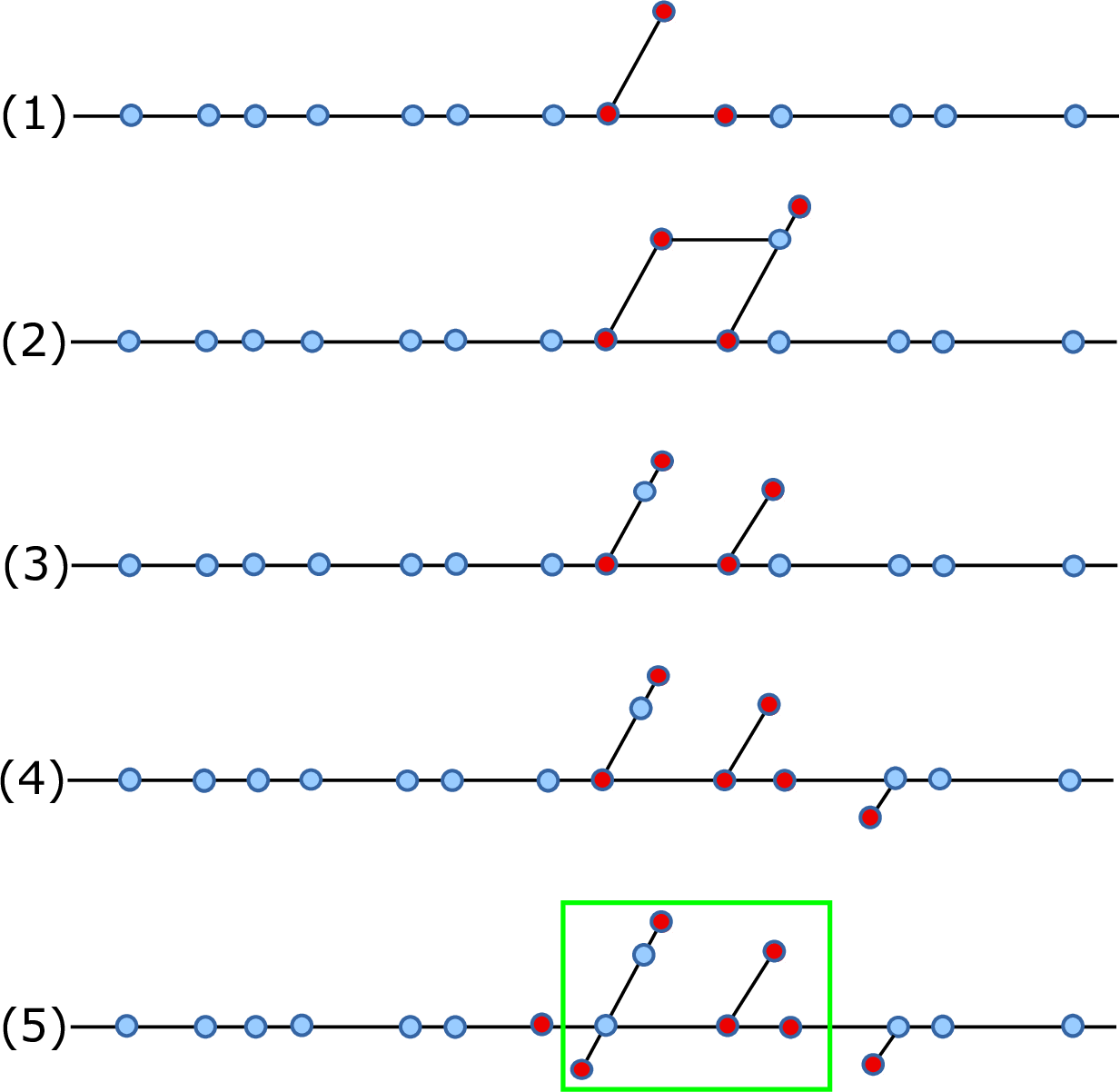
To put more intersection points of on , we can insert a single next to . On the left side of , we need to insert to make a single dot. Hence, if there is no smaller index of , the green box in Figure 15 contains a local optimal pattern.
2pt \pinlabel at 393 638 \pinlabel at 470 638
at 393 490 \pinlabel at 470 490
at 393 345 \pinlabel at 470 345
at 393 203 \pinlabel at 465 203 \pinlabel at 510 203
at 353 50 \pinlabel at 405 50 \pinlabel at 375 15 \pinlabel at 465 50 \pinlabel at 505 50
2pt \pinlabel at 395 715 \pinlabel at 490 715 \pinlabel at 470 693
at 395 570 \pinlabel at 475 570 \pinlabel at 525 570 \pinlabel at 490 544
at 395 420 \pinlabel at 475 420 \pinlabel at 525 420 \pinlabel at 490 392
at 395 250 \pinlabel at 475 250 \pinlabel at 525 250 \pinlabel at 490 225
at 400 90 \pinlabel at 375 62 \pinlabel at 473 85 \pinlabel at 522 90 \pinlabel at 485 62
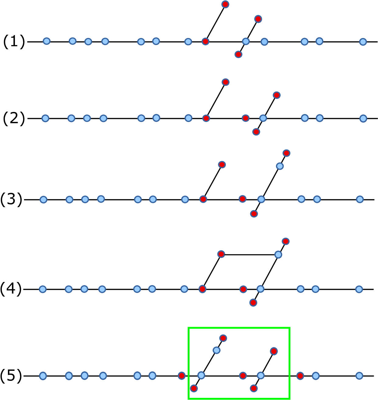
On the other hand, if does have , then we can insert an additional as illustrated in (2) of Figure 16. That means the additional is and the original becomes . The (3) and (4) in Figure 16 show that the next ascending segment should be lower. Otherwise, a degenerate hexagon surgery occurs. To reduce the indices slowly, the highest index of the ascending segment should be one less. The green box in Figure 16 contains another local optimal pattern.
Both local optimal patterns have three ’s, one of which is a single dot, and the other two are in two ascending segments. The highest index of the right one is exactly one less than that of the left one. The difference lies in the number of ’s. The first pattern only contains a single , while the second one has two ’s.
To put it simple, if we iterate the two patterns independently, we will have the top illustrations in Figures 17 & 18. The violation of hexagon surgery forces the highest index of ascending segments is larger than that on the right. To be optimal, the highest indices decrease exactly one as we move along. If we extend the graph below , we will observe a big difference between the two patterns.
In the first pattern, since there is only one in each pattern, it is unnecessary to add more or except for the rightmost ascending segment. It will violate the efficiency if we don’t put an . The situation is quite different in the second pattern, as a hexagon surgery occurs in each pattern. To get rid of all these surgeries, we add the ascending segments as in Figure 18. In comparison to the previous pattern, it will significantly increase the distance, so it is not the worst scenario. It follows that the worst case only consists of the first pattern. Generally, two patterns can be mixed, but each second pattern will add more curves in the rainbow. Hence, the worst scenario only contains the first pattern.
With this in mind, we define the function to be the difference of the highest index and the lowest index in Figure 17 type pattern that has dots at . Same to the first rainbow, we can construct a new curve by the subarc and , denoted as . It follows that , because . Each pattern has three dots, so we have the following three cases for .
In Figure 17, the intersection number , and we have . When , we can remove the rightmost ascending segment, as shown in Figure 19. In this case, . When , either we can add a leftmost ascending segment, or add two leftmost ascending segment and remove the rightmost one. Figure 20 illustrates this case, but we have for both cases.
More generally, the formula of is as follows.
| (17) |
∎
7. Proof of super efficiency
Now we can repeat our previous calculations in section 5 to prove the main theorem.
Proof of Theorem 1.1.
For the case , substituting for on the right and for on the left in equation 15, we get
| (18) |
In the case of , the solution is , so .
Let us deal with the other two cases. When ,
| (19) |
In the case that , the solution is , so . It is for , so .
The other case is , and we have
| (20) |
The solution is , so for .
Now returning to our previous equation 15 calculation, we need to raise the value of from to for . To do this we need .
For genus , our equations to solve are
| (21) |
| (22) |
| (23) |
For the three cases, the solutions are , and , then , and , respectively.
Now returning back to our previous equation 14 calculation, we need to raise the value of from to . To do this we need , for . Then we have our result that the geodesic of minimal complexity is initially super efficient with the stated bound.
∎
Remark 7.1.
Proof of Corollary 1.2.
Let and be pairwise minimal intersecting representatives of and without any triple points. For the polygons in that are non-hexagons, we can cut through them along some reference arcs to make them to be hexagons. With this in mind, we end up with polygons that are the rectangles and hexagons. By Euler characteristic calculation, there are hexagons. Since the reference arcs in rectangles are parallel to the adjacent ones in the hexagons, then they are only counted once. It implies that there are reference arcs in total. Up to homotopy, the intersection number of with each reference arc determines . By Theorem 1.1, the choice of intersection number is at most for each reference arc, so there are at most candidates for . For , the number of candidates is .
∎
8. subsection: algorithm
Continuing our discussion of § 1.5 concerning the implementation of a distance algorithm utilizing super efficient geodesics, the key calculation is resolving the value of for the equation 14. We finally settle on as the smallest needed value when calculating the solution to equation 19. Thus, we have the geometric condition that there must be fewer than parallel arcs of so as to prevent that growth of parallel arcs of , and other . This seems a very checkable condition for candidates of . Viewed from this perspective and observing that this condition is independent of genus, the linear bounds on in Theorem 1.1 can be misleading. Independent of distance and genus, the first step in distance algorithm based upon super efficient geodesics would be to produce a list of candidate curves for with the requirement, that with respect to any reference arc, there are fewer than parallel arcs as understood in statement of Proposition 6.1.
Seen from this perspective, super efficient geodesics achieve a high degree of economy in both variables of distance and genus. The cost of guaranteeing at least sixteen parallel arcs comes from the application of the pigeonhole principle as stated in the last sentence of the proof of Proposition 6.1.
Having a universal bound—independent of distance and genus—on the number of parallel arcs of , for some reference arc, is striking. At the moment there is no proof of -hyperbolic utilizing the technology of efficient geodesics. We know from [1, 6] that there is a uniform , independent of genus. Possessing this common attribute of universality, it is tempting to speculate that can be leveraged to produce an efficient-geodesic-proof of hyperbolicity of the curve complex.
References
- [1] Tarik Aougab. Uniform hyperbolicity of the graphs of curves. Geom. Topol., 17 (2013), no. 5, 2855 - 2875.
- [2] Taik Aougab, S. Huang. Minimally intersecting filling pairs on surfaces. Algebraic Geom. Topol., 15 (2015), 903?932.
- [3] Tarik Aougab, Priyam Patel, Samuel J. Taylor. Covers of surfaces, Kleinian groups, and the curve complex. https://arxiv.org/abs/1810.12953
- [4] Mark C. Bell and Richard C. H. Webb. Polynomial-time algorithms for the curve graph. https://arxiv.org/abs/1609.09392
- [5] Joan Birman, Dan Margalit, and William Menasco. Efficient geodesics and an effective algorithm for distance in the complex of curves. Math. Ann., 366:1253–1279, 2016.
- [6] Brian H. Bowditch. Uniform hyperbolicity of the curve graphs. Pacific J. Math., 269(2):269–280, 2014.
- [7] Paul Glenn, William W. Menasco, Kayla Morrell, and Matthew Morse. Metric In The Curve Complex. software, available at micc.github.io, 2014.
- [8] Paul Glenn, William W. Menasco, Kayla Morrell, and Matthew Morse. MICC: A Tool For Computing Short Distances In The Curve Complex. Journal of Symbolic Computation, Special issue on Algorithms and Software for Computational Topology:115–132, 2017.
- [9] William J. Harvey. Boundary structure of the modular group. pages 245–251, 1981. in: Riemann surfaces and related topics. Proceedings of the 1978 Stony Brook Conference (Stony Brook 1978), Ann. of Math. Stud. 97,.
- [10] John Hempel. 3-manifolds as viewed from the curve complex. Topology, 40:631–657, 2001.
- [11] Jason Paige Leasure. Geodesics in the complex of curves of a surface. ProQuest LLC, Ann Arbor, MI, 2002. Thesis (Ph.D.)–The University of Texas at Austin.
- [12] Howard A. Masur and Yair N. Minsky. Geometry of the complex of curves. I. Hyperbolicity. Invent. Math., 138(1):103–149, 1999.
- [13] Howard A. Masur and Yair N. Minsky. Geometry of the complex of curves II: Hierarchical Structure. Geom. Funct. Anal. 10 (2000), no. 4, 902 - 974.
- [14] Kenneth J. Shackleton. Tightness and computing distances in the curve complex. Geom. Dedicata, 160:243–259, 2012.
- [15] Yohsuke Watanabe. Intersection numbers in the curve graph with a uniform constant. Topology Appl., 204:157–167, 2016.
- [16] Richard C. H. Webb. Combinatorics of tight geodesics and stable lengths. Trans. Amer. Math. Soc., 367(10):7323–7342, 2015.