Low-complexity Architecture for AR(1) Inference

Due to the raising demand for digital signal processing (DSP) systems capable of operating at low power and low complexity, approximate methods have been considered for image processing [7, 5]. In particular, several approximate discrete transforms have been recently proposed [14, 6, 18] for image compression, where pixel data often stems from natural images and are modeled according to the first order autoregressive ($\operatorname{AR(1)}$) process [12]. The $\operatorname{AR}(1)$ model depends only on a single parameter, the correlation coefficient $\rho$, whose identification determines the suitable DSP tools for data analysis [3, 11]. In particular, image sensor networks and mobile computing systems may benefit from low-complexity fundamental DSP building blocks [2]. In this Letter, we aim at the derivation of a low-complexity algorithm for the estimation of $\rho$ targeting its implementation on embedded, low-power devices.

A real-valued, discrete-time, wide-sense stationary stochastic process $\{X_{n},n=1,2,\ldots\}$ with null mean and finite variance is said to be an $\operatorname{AR}(1)$ process if

where $|\rho|<1$ and $W_{n}$ is a white noise process independent of $X_{n}$. If the joint distribution of any finite set of samples from (1) is Gaussian, then we say that $X_{n}$ is a Gaussian $\operatorname{AR(1)}$ process. Assuming stationarity of $X_{n}$, its autocorrelation function is given by $\mathrm{cor}(X_{n},X_{m})=\rho^{|n-m|}$, which depends solely on $\rho$. The traditional estimator for $\rho$ is given by [9, p. 77]:

Hereafter we refer to the above statistic as the autocorrelation function (ACF) estimator [9].

A binary threshold process derived from $X_{n}$ is defined according to $S_{n}=I(X_{n}>0)$, where $I(\cdot)$ equals $1$ if its argument is true and $0$ otherwise. We refer to $S_{n}$ as the signed $\operatorname{AR}(1)$ process. The following theorem proposed by Kedem [10] relates $\rho$ to the stochastic structure of $S_{n}$.

The unbiased maximum likelihood estimator (MLE) of $\lambda$ is based on $S_{1},S_{2},\ldots,S_{N}$ and is given by

Invoking the Invariance Principle [4], the MLE for $\rho$ is derived from (3) and is given by $\rho(\hat{\lambda}_{N})$. We refer to it as the Kedem estimator.

A low-complexity estimator for $\rho$ can be derived by means of approximating the function $\rho(\lambda)$ in (3). By using global and convex optimization [13, 8], we obtain the optimal 5-interval piecewise linear approximation for $\rho(\lambda)$ in (3), furnishing the following proposed low-complexity estimator:

The absolute error satisfies: $|\tilde{\rho}(\lambda)-\rho(\lambda)|<1.4\cdot 10^{-2}$. The proposed approximate estimator is therefore $\tilde{\rho}(\hat{\lambda}_{N})$.

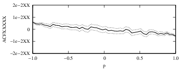
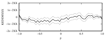
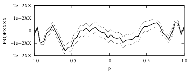
A Monte Carlo simulation with $R=1000$ replicates of the $\operatorname{AR}(1)$ process of length $N=512$ was used to assess behavior of the proposed estimator in comparison with the ACF estimator. The selected values of $\rho$ were $\rho\in[-1,1]$ in steps of $4\cdot 10^{-2}$. The power of the additive white noise in (1) was adjusted such that $90\%$ of its realizations are within $[-1,1]$, resulting in $W_{n}\sim\mathcal{N}(0,0.61)$. In order to quantify the performance of the proposed low complexity estimator compared to the ACF estimator in (2), we computed $\hat{\rho}_{N}^{(r)}-\rho$, $\rho^{(r)}(\hat{\lambda}_{N})-\rho$, and $\tilde{\rho}_{N}^{(r)}(\hat{\lambda}_{N})-\rho$ for each replicate $r=0,1,\ldots,R-1$, where $\hat{\rho}_{N}^{(r)}$, $\rho^{(r)}(\hat{\lambda}_{N})$, and $\tilde{\rho}^{(r)}(\hat{\lambda}_{N})$ are the estimates of $\rho$ according to the ACF, Kedem, and the proposed estimators for each replicate $r$, respectively. Fig. 1 displays values of $\operatorname{err}(\hat{\rho}_{N})=\sum_{r=1}^{R}(\hat{\rho}_{N}^{(r)}-\rho)/R$, $\operatorname{err}(\rho(\hat{\lambda}_{N}))=\sum_{r=1}^{R}(\rho^{(r)}(\hat{\lambda}_{N})-\rho)/R$, and $\operatorname{err}(\tilde{\rho}(\hat{\lambda}_{N}))=\sum_{r=1}^{R}(\tilde{\rho}^{(r)}(\hat{\lambda}_{N})-\rho)/R$ along with the $95\%$ confidence intervals based on the normal distribution.

The direct implementation of the ACF estimator requires one division, $2N$ multiplications, $2N-1$ additions. Assuming that $\hat{\lambda}_{N}$ is known, the estimator for $\rho$ derived from Theorem 1 requires one addition, one multiplication by $\pi$, and one call of the cosine function. The cosine function is implemented through the coordinated rotation digital computer (CORDIC) algorithm, which is an iterative method that employs successive additions of bit-shifted quantities. Each iteration of the CORDIC algorithm requires two additions and two shifts at most, depending on the the angles that are computed. The implementation of the CORDIC block used in the the proposed architectures require 14 iterations [16, pg. 40], resulting in a total of 28 additions and up to 28 bit-shifts for each evaluation of the cosine function. On its turn, the computation of $\hat{\lambda}_{N}$ requires $N-1$ additions, $N-1$ comparisons, and one division by $N-1$. On the other hand, given that $\hat{\lambda}_{N}$ is available, the proposed approximate estimator $\tilde{\rho}(\hat{\lambda}_{N})$ based on (5) requires only multiplications by simple constants, additions and bit-shifting operations, amounting to $N+1$ additions and at most $2$ shifts. as well as a comparator. Table 1 summarizes the arithmetic complexity for the ACF, Kedem, and the proposed estimator.

The ACF, Kedem, and the proposed approximate estimator were implemented on a Xilinx Artix-7 XC7A35T-1CPG236C FPGA device. Although there are different architectures for digital correlators based on fast Fourier transforms (FFT) for different applications [1], we choose not to implement such scheme given its higher complexity in terms of resources and power compared to the architecture in Fig. 2. The implementations are capable of providing an estimate of $\rho$ for every clock pulse using the last $N$ input samples. The ACF estimator in (2) was implemented using the architecture depicted in Fig. 2. The structure for computing $\hat{\rho}_{N}$ possesses two identical $(N-1)$-sample delay lines after the computation of $X_{n}X_{n-1}$ and $X_{n}X_{n}$. The values of $X_{n}X_{n-1}$ and $X_{n}X_{n}$ in $N-1$ cycles in the past are subtracted from the current value of $\sum_{n=2}^{N}X_{n}X_{n-1}$ and $\sum_{n=1}^{N}X_{n}X_{n}$, respectively. This scheme allows the overall system to compute the correlation limited to the last $N$ samples. Without the delay network, the circuit would yield the correlation for the whole sequence from its beginning and incur in overflow.

The Kedem and the proposed estimators share the structure shown in Fig 3, which is required for computing the estimated value of $\lambda$. The input word representing the samples in time in Fig. 3 is downsized from $B=10$ bits to the sign bit. The current sign bit is then compared to the sign bit of the last sample and the result is stored in a shift register of size $N$. We adopted $N=512$. Subsequently the output sequence from the comparator is shifted to the right at every rising edge of the clock. The value of $\hat{\lambda}$ is then added to the net value of the immediate sign bit comparison and the comparison $N$ clock periods earlier. Note that this delay network is the same present on Fig. 2, allowing the design to account for only a window of size $N$. This negative loop results in forcing $\hat{\lambda}$ to store the number of comparisons that were evaluated as true in the last $N$ clock pulses, including the current sample compared to the previous one.

Such estimated value $\hat{\lambda}_{N}$ is then submitted to the block implementing the functions $\rho(\cdot)$ or $\tilde{\rho}(\cdot)$ for the Kedem or the proposed estimator, respectively. For the Kedem estimator, a single call for the cosine function is required, being physically implemented according to the Xilinx implementation of the CORDIC algorithm as described in [16, p. 17].

In terms of the proposed estimator, aiming at a low-cost hardware implementation, the constants required in (5) were approximated according to dyadic integers with low magnitude numerator, rendering the values in Table 2. The computation of $\tilde{\rho}(\lambda)$ is depicted in Fig. 4. Pipeline stages are not shown for simplicity. The mux block in Fig. 4 selects the appropriate path according to the interval defined in (5). The symmetry of $\tilde{\rho}(\lambda)$ was exploited in such a way that the slope coefficients in the first three intervals were sufficient for the computing $\tilde{\rho}(\lambda)$ for all possible values of $\lambda$.

The designs were implemented using a signed 10-bit word for representing the the output estimates according to the ACF, Kedem, and the proposed estimator. Table 3 summarizes the resource utilization in terms of look-up table (LUT), flip-flops (FF), and slices [17] and performance measurements expressed by maximum operating frequency, latency, and dynamic power. The percentages in parenthesis inform the variations compared to the ACF estimator. The proposed design offers significant savings in resource consumption: (i) the number of LUTs, latency, and dynamic power were dramatically reduced in more than 93% compared to the exact implementation of the estimator. The number of FFs and slices were reduced in more than 75%; and the maximum operating frequency received a two-fold increase. The significant reduction in the latency of the design based on (3) is mainly due to the absence of multipliers and dividers [15], which demand several clock cycles to complete an operation. In particular, the proposed design shows better metrics because the consecutive shift-and-add operations of the CORDIC [16] block, employed to compute the cosine, are substituted by multiplications by hardware-friendly constants, requiring just a few shifts and additions.

A low-complexity approximate method for computing the correlation coefficient in $\operatorname{AR}(1)$ processes was introduced. Numerical simulations indicate the good performance of the proposed estimator when compared with the standard method in literature. The associate computational complexity favors its implementation in low-power hardware. Hardware implementation metrics of the proposed estimator are shown to be much more attractive than the ones resulting from the ACF estimator architecture. In particular, the dynamic power of the implementation of the proposed method is almost fourteen times smaller than the traditional method, while the the maximum operating frequency is doubled.

This work has been partially supported by CNPq, Brazil, and NSERC, Canada.

References

- [1] V. R. Balu and S. M. R. Hasan, Computationally minimized x-part for FX correlator in big-data interferometers, IEEE Access, 5 (2017), pp. 25353–25364.
- [2] F. Betzel, K. Khatamifard, H. Suresh, D. J. Lilja, J. Sartori, and U. Karpuzcu, Approximate communication: Techniques for reducing communication bottlenecks in large-scale parallel systems, ACM Computing Surveys (CSUR), 51 (2018), p. 1.
- [3] V. Britanak, P. Yip, and K. R. Rao, Discrete Cosine and Sine Transforms, Academic Press, 2007.
- [4] G. Casella and R. L. Berger, Statistical Inference, vol. 2, Duxbury Pacific Grove, CA, 2002.
- [5] R. J. Cintra and F. M. Bayer, A DCT approximation for image compression, IEEE Signal Processing Letters, 18 (2011), pp. 579–582.
- [6] V. de A. Coutinho, R. J. Cintra, and F. M. Bayer, Low-complexity multidimensional DCT approximations for high-order tensor data decorrelation, IEEE Transactions on Image Processing, 26 (2017), pp. 2296–2310.
- [7] T. I. Haweel, A new square wave transform based on the DCT, Signal processing, 81 (2001), pp. 2309–2319.
- [8] C. F. Jekel and G. Venter, pwlf: A Python Library for Fitting 1D Continuous Piecewise Linear Functions, 2019.
- [9] S. M. Kay, Modern Spectral Estimation, Prentice-Hall, Upper Saddle River, NJ, 1988.
- [10] B. Kedem, Estimation of the parameters in stationary autoregressive processes after hard limiting, Journal of the American Statistical Association, 75 (1980), pp. 146–153.
- [11] M. T. Pourazad, C. Doutre, M. Azimi, and P. Nasiopoulos, HEVC: The new gold standard for video compression: How does HEVC compare with H.264/AVC?, IEEE Consumer Electronics Magazine, 1 (2012), pp. 36 – 46.
- [12] K. R. Rao and P. Yip, Discrete Cosine Transform: Algorithms, Advantages, Applications, Academic press, 2014.
- [13] R. Storn and K. Price, Differential evolution – a simple and efficient heuristic for global optimization over continuous spaces, Journal of Global Optimization, 11 (1997), pp. 341–359.
- [14] C. J. Tablada, F. M. Bayer, and R. J. Cintra, A class of DCT approximations based on the Feig-Winograd algorithm, Signal Processing, 113 (2015), pp. 38–51.
- [15] Xilinx, Divider Generator v5.1 LogiCORE IP Product Guide, Oct. 2016.
- [16] , CORDIC v6.0 LogiCORE IP Product Guide, 2017.
- [17] , 7 Series DSP48E1 Slice User Guide, Mar. 2018.
- [18] X. Zhao, G. An, Y. Cen, H. Wang, and R. Zhao, Robust generalized low rank approximations of matrices for video denoising, in 2016 IEEE 13th International Conference on Signal Processing (ICSP), Nov 2016, pp. 815–818.